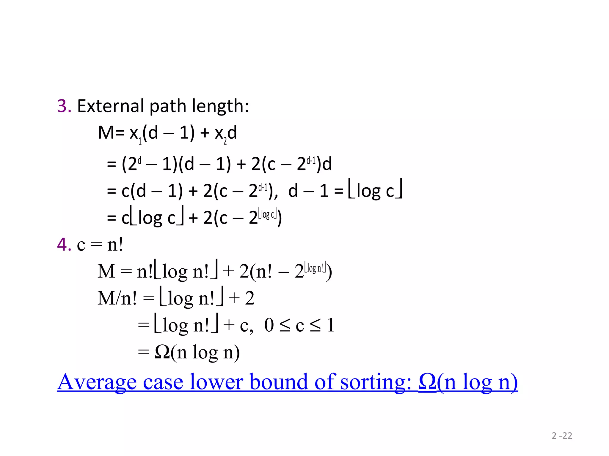
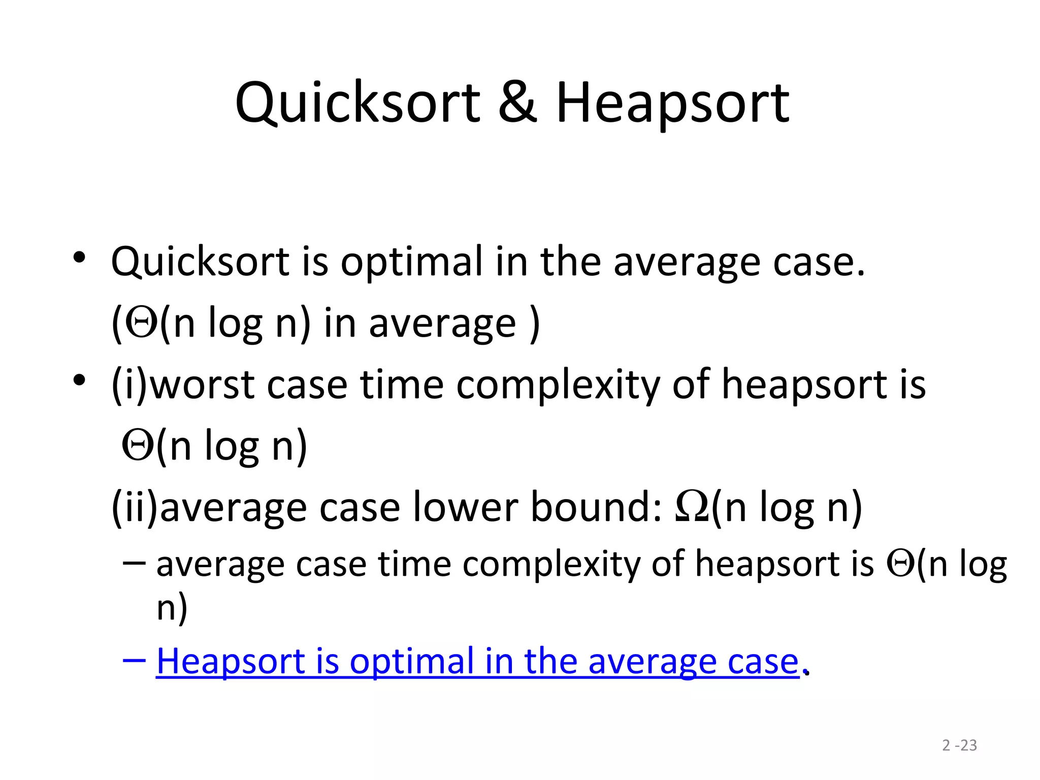
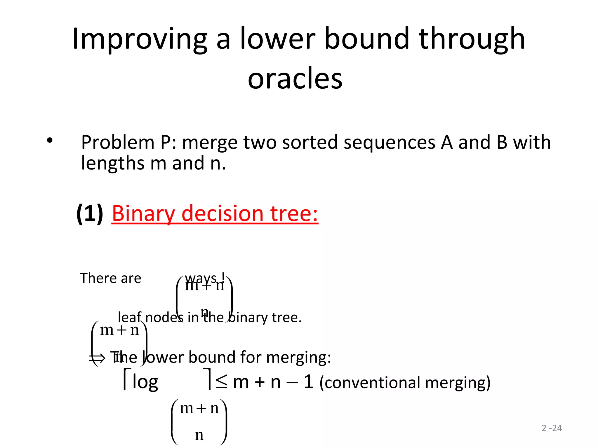
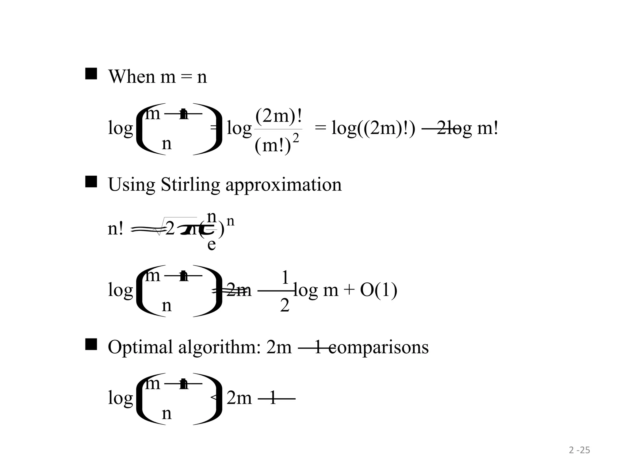
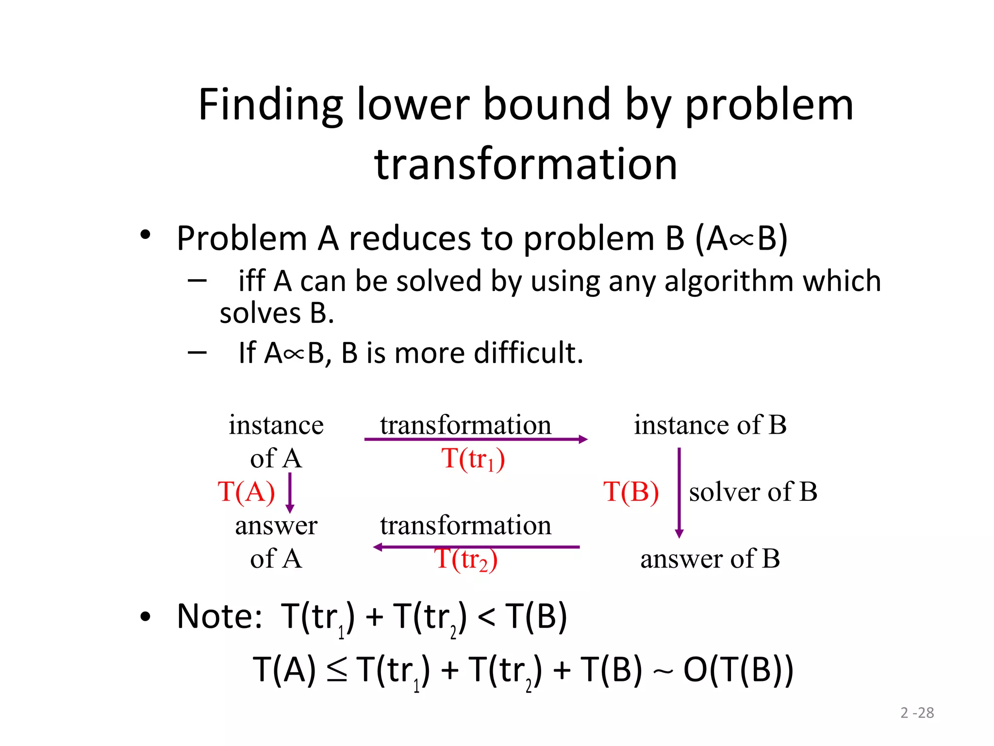
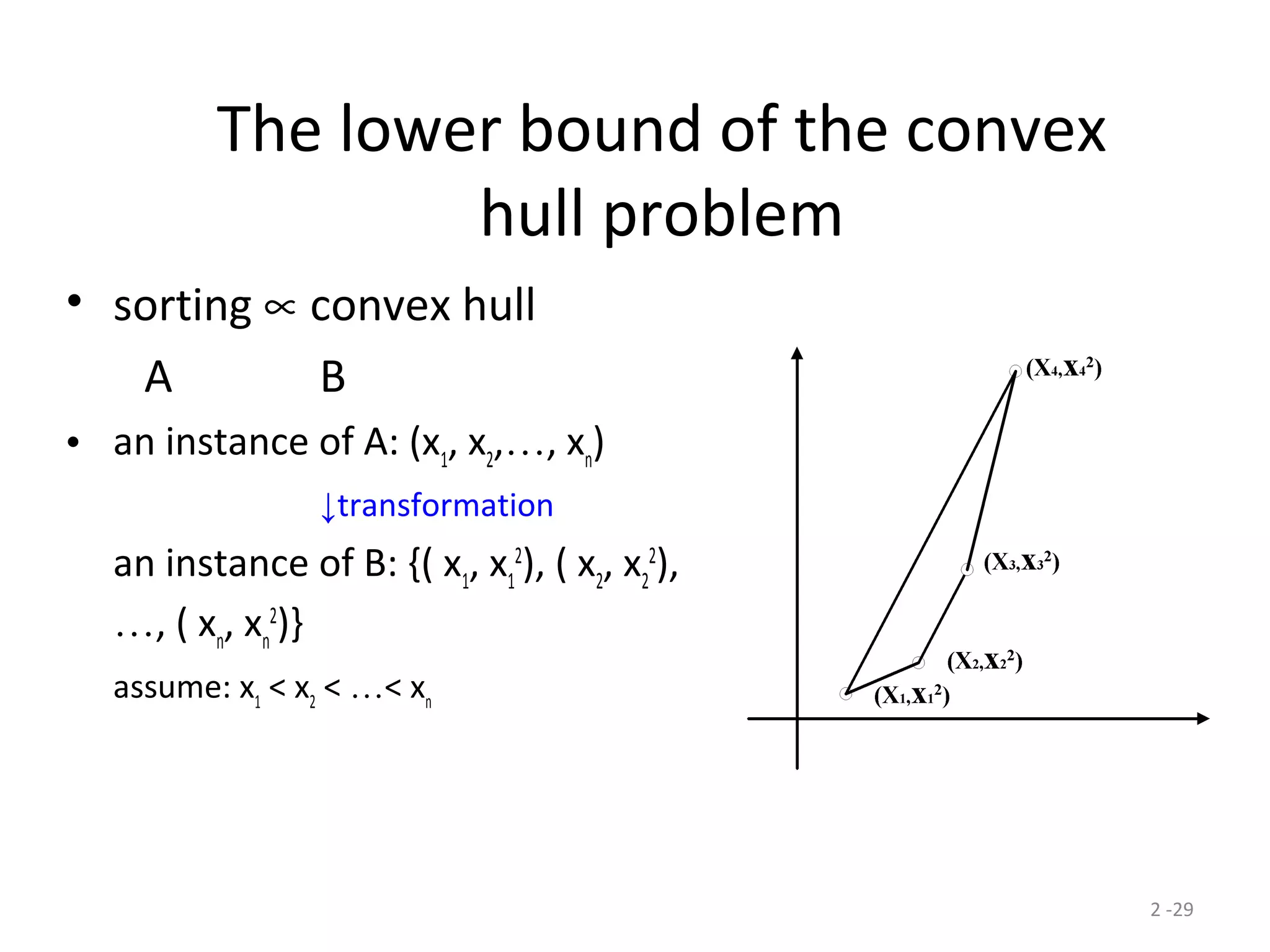
The document discusses lower bounds for sorting algorithms. It shows that the worst case and average case lower bounds for sorting are both Ω(n log n). This lower bound is derived by analyzing the minimum depth of balanced binary decision trees required to represent the n! possible permutations of n elements. Several algorithms, including heapsort, are shown to achieve the optimal time complexity of O(n log n), matching this lower bound. Problem transformations are also introduced as a method for proving lower bounds.

1. Algorithms
Divide And Conquer -Surfing Lower
Bounds

2. 2 -2
Lower bound
• Def : A lower bound of a problem is the least time
complexity required for any algorithm which can be used
to solve this problem.
☆ worst case lower bound
☆ average case lower bound
• The lower bound for a problem is not unique.
– e.g. Ω(1), Ω(n), Ω(n log n) are all lower bounds for
sorting.
– (Ω(1), Ω(n) are trivial)

3. 2 -3
• At present, if the highest lower bound of a problem
is Ω(n log n) and the time complexity of the best
algorithm is O(n2
).
– We may try to find a higher lower bound.
– We may try to find a better algorithm.
– Both of the lower bound and the algorithm may be
improved.
• If the present lower bound is Ω(n log n) and there
is an algorithm with time complexity O(n log n),
then the algorithm is optimal..

4. 2 -4
6 permutations for 3 data elements
a1
a2
a3
1 2 3
1 3 2
2 1 3
2 3 1
3 1 2
3 2 1
The worst case lower bound of sorting

5. 2 -5
Straight insertion sort:
• input data: (2, 3, 1)
(1) a1
:a2
(2) a2
:a3
, a2
↔a3
(3) a1
:a2
, a1
↔a2
• input data: (2, 1, 3)
(1)a1
:a2
, a1
↔a2
(2)a2
:a3

6. 2 -6
Decision tree for straight insertion sort

7. 2 -7
Decision tree for bubble sort

8. 2 -8
Lower bound of sorting
• To find the lower bound, we have to find the
smallest depth of a binary tree.
• n! distinct permutations
n! leaf nodes in the binary decision tree.
• balanced tree has the smallest depth:
log(n!) = Ω(n log n)
lower bound for sorting: Ω(n log n)

9. 2 -9
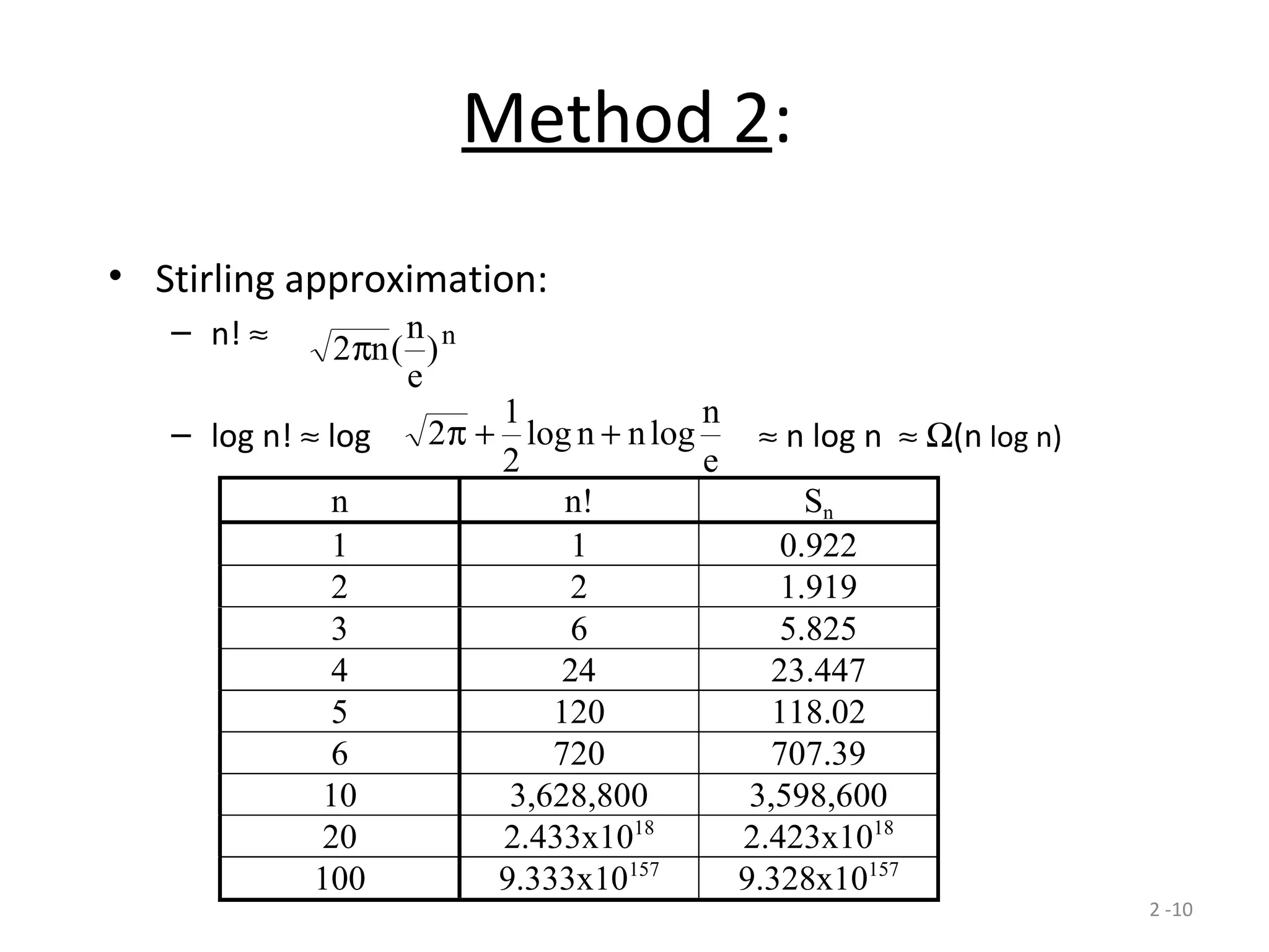
Method 1:
log(n!) = log(n(n− 1)…1)
= log2 + log3 +…+ log n
> log xdx
n
1∫
= log e ln xdx
n
1∫
= log e[ ln ]x x x n
− 1
= log e(n ln n − n + 1)
= n log n − n log e + 1.44
≥ n log n − 1.44n
=Ω (n log n)

10. 2 -10
Method 2:
• Stirling approximation:
– n! ≈
– log n! ≈ log ≈ n log n ≈ Ω(n log n)
2πn
n
e
n
( )
2
1
2
π + +log logn n
n
e
n n! Sn
1 1 0.922
2 2 1.919
3 6 5.825
4 24 23.447
5 120 118.02
6 720 707.39
10 3,628,800 3,598,600
20 2.433x1018
2.423x1018
100 9.333x10157
9.328x10157

11. 2 -11
)A(
),i-(
A(i)
A(i)):A(
)A(
ni:
A(i)
A(i)
),...,A(n)),A(A(
1Output
End
11Restore
Delete
1
1Output
Begin
do2down toFor
s.'ofsequencesortedThe:Ouput
d.constructealreadyheapaofnodeaiseacherewh
21:Input
Heapsort7-2Algorithm
=
=

12. 2 -12
Heapsort—An optimal sorting algorithm
• A heap : parent ≥ son

13. 2 -13
• output the maximum and restore:
• Heapsort: construction
output

14. 2 -14
Phase 1: construction
• input data: 4, 37, 26, 15, 48 • restore the subtree rooted at
A(2):
• restore the tree rooted at
A(1):

15. 2 -15
Phase 2: output

16. 2 -16
Implementation
• using a linear array
not a binary tree.
– The sons of A(h) are A(2h) and A(2h+1).
• time complexity: O(n log n)

17. 2 -17
Time complexity
Phase 1: construction
d = log n: depth
# of comparisons is at most:
L
d
=
−
∑
0
1
2(d−L)2L
=2d
L
d
=
−
∑
0
1
2L
−4
L
d
=
−
∑
0
1
L2L-1
(
L
k
=
∑
0
L2L-1
= 2k
(k−1)+1)
=2d(2d
−1) −4(2d-1
(d −1 −1) + 1)
:
= cn −2log n−4, 2 ≤c ≤4
d
L
d-L

18. 2 -18
Time complexity
Phase 2: output
2
i
n
=
−
∑
1
1
log i
= :
=2nlog n−4cn + 4, 2 ≤c ≤4
=O(n log n)
log i
i nodes

19. 2 -19
Average case lower bound of sorting
• By binary decision tree
• The average time complexity of a sorting algorithm:
the external path length of the binary tree
n!
• The external path length is minimized if the tree is
balanced.
(all leaf nodes on level d or level d−1)

20. 2 -20
unbalanced
external path length
= 4⋅3 + 1 = 13
balanced
external path length
= 2⋅3+3⋅2 = 12
Average case lower bound of sorting

21. 2 -21
Compute the min external path length
1. Depth of balanced binary tree with c leaf nodes:
d = log c
Leaf nodes can appear only on level d or d−1.
2. x1
leaf nodes on level d−1
x2
leaf nodes on level d
x1
+ x2
= c
x1
+ = 2d-1
⇒ x1
= 2d
−c
d-1
x2
2

22. 2 -22
3. External path length:
M= x1
(d − 1) + x2
d
= (2d
− 1)(d − 1) + 2(c − 2d-1
)d
= c(d − 1) + 2(c − 2d-1
), d − 1 = log c
= clog c + 2(c − 2logc
)
4. c = n!
M = n!log n! + 2(n! − 2logn!
)
M/n! = log n! + 2
= log n! + c, 0 ≤ c ≤ 1
= Ω(n log n)
Average case lower bound of sorting: Ω(n log n)

23. 2 -23
Quicksort & Heapsort
• Quicksort is optimal in the average case.
(Θ(n log n) in average )
• (i)worst case time complexity of heapsort is
Θ(n log n)
(ii)average case lower bound: Ω(n log n)
– average case time complexity of heapsort is Θ(n log
n)
– Heapsort is optimal in the average case..

24. 2 -24
Improving a lower bound through
oracles
• Problem P: merge two sorted sequences A and B with
lengths m and n.
(1) Binary decision tree:
There are ways !
leaf nodes in the binary tree.
⇒ The lower bound for merging:
log  ≤ m + n − 1 (conventional merging)
m n
n
+





m n
n
+





m n
n
+






25. 2 -25
When m = n
log
m n
n
+




= log
( )!
( !)
2
2
m
m
= log((2m)!) −2log m!
Using Stirling approximation
n! ≈2πn
n
e
n
( )
log
m n
n
+




≈2m −
1
2
log m + O(1)
Optimal algorithm: 2m −1 comparisons
log
m n
n
+




< 2m −1

26. 2 -26
(2) Oracle:
• The oracle tries its best to cause the algorithm
to work as hard as it might. (to give a very hard
data set)
• Sorted sequences:
– A: a1
< a2
< … < am
– B: b1
< b2
< … < bm
• The very hard case:
– a1
< b1
< a2
< b2
< … < am
< bm

27. 2 -27
• We must compare:
a1
: b1
b1
: a2
a2
: b2
:
bm-1
: am-1
am
: bm
• Otherwise, we may get a wrong result for some input data.
e.g. If b1
and a2
are not compared, we can not distinguish
a1
< b1
< a2
< b2
< … < am
< bm
and
a1
< a2
< b1
< b2
< … < am
< bm
• Thus, at least 2m−1 comparisons are required.
• The conventional merging algorithm is optimal for m = n.

28. 2 -28
Finding lower bound by problem
transformation
• Problem A reduces to problem B (A∝B)
– iff A can be solved by using any algorithm which
solves B.
– If A∝B, B is more difficult.
• Note: T(tr1
) + T(tr2
) < T(B)
T(A) ≤ T(tr1
) + T(tr2
) + T(B) ∼ O(T(B))
instance
of A
transformation
T(tr1)
instance of B
T(A) T(B) solver of B
answer
of A
transformation
T(tr2) answer of B

29. 2 -29
The lower bound of the convex
hull problem
• sorting ∝ convex hull
A B
• an instance of A: (x1
, x2
,…, xn
)
↓transformation
an instance of B: {( x1
, x1
2
), ( x2
, x2
2
),
…, ( xn
, xn
2
)}
assume: x1
< x2
< …< xn

30. 2 -30
• If the convex hull problem can be solved,
we can also solve the sorting problem.
– The lower bound of sorting: Ω(n log n)
• The lower bound of the convex hull
problem: Ω(n log n)

31. 2 -31
The lower bound of the Euclidean minimal
spanning tree (MST) problem
• sorting ∝ Euclidean MST
A B
• an instance of A: (x1
, x2
,…, xn
)
↓transformation
an instance of B: {( x1
, 0), ( x2
, 0),…, ( xn
, 0)}
– Assume x1
< x2
< x3
<…< xn
– ⇔there is an edge between (xi
, 0) and (xi+1
, 0) in
the MST, where 1 ≤ i ≤ n−1

32. 2 -32
• If the Euclidean MST problem can be
solved, we can also solve the sorting
problem.
– The lower bound of sorting: Ω(n log n)
• The lower bound of the Euclidean MST
problem: Ω(n log n)