Divide and ConquerTechnique
General Method:
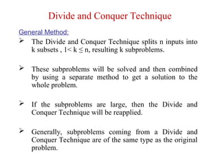
The Divide and Conquer Technique splits n inputs into
k subsets , 1< k ≤ n, resulting k subproblems.
These subproblems will be solved and then combined
by using a separate method to get a solution to the
whole problem.
If the subproblems are large, then the Divide and
Conquer Technique will be reapplied.
Generally, subproblems coming from a Divide and
Conquer Technique are of the same type as the original
problem.
3.
The reapplicationof the Divide and Conquer
Technique is naturally expressed by a recursive
algorithm.
Now smaller and smaller problems of the same kind
are generated until subproblems that are small enough
to solve without splitting further.
4.
• Divide theproblem into a number of sub-problems
– Similar sub-problems of smaller size
• Conquer the sub-problems
– Solve the sub-problems recursively
– Sub-problem size small enough -> solve the problems in
straightforward manner
• Combine the solutions of the sub-problems
– Obtain the solution for the original problem
5.
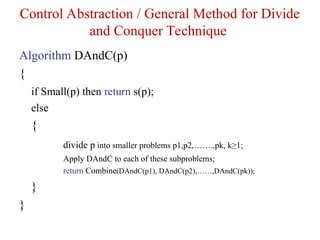
Control Abstraction /General Method for Divide
and Conquer Technique
Algorithm DAndC(p)
{
if Small(p) then return s(p);
else
{
divide p into smaller problems p1,p2,…….,pk, k≥1;
Apply DAndC to each of these subproblems;
return Combine(DAndC(p1), DAndC(p2),……,DAndC(pk));
}
}
6.
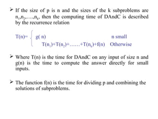
If thesize of p is n and the sizes of the k subproblems are
n1,n2,….,nk, then the computing time of DAndC is described
by the recurrence relation
T(n)= g( n) n small
T(n1)+T(n2)+……+T(nk)+f(n) Otherwise
Where T(n) is the time for DAndC on any input of size n and
g(n) is the time to compute the answer directly for small
inputs.
The function f(n) is the time for dividing p and combining the
solutions of subproblems.
7.
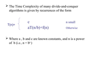
The TimeComplexity of many divide-and-conquer
algorithms is given by recurrences of the form
c n small
aT(n/b)+f(n) Otherwise
Where a , b and c are known constants, and n is a power
of b (i.e., n = bk
)
T(n)=
8.
Examples
Merge Sort: T(n)= 2T(n/2) + Cn
The solution is Θ(n Logn)
Binary Search: T(n) = T(n/2) + C.
The solution is Θ(Logn)
9.
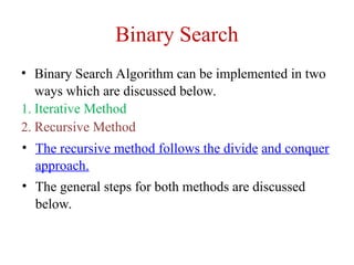
Binary Search
• BinarySearch Algorithm can be implemented in two
ways which are discussed below.
1. Iterative Method
2. Recursive Method
• The recursive method follows the divide and conquer
approach.
• The general steps for both methods are discussed
below.
10.
Iterative Method
Algorithm BinSearch(a,n, x)
// a is an array of size n, x is the key element to be searched.
{ low:=1; high:=n;
while( low ≤ high)
{
mid:=(low+high)/2;
if( x < a[mid] ) then high := mid-1;
else if( x > a[mid] ) then low := mid+1;
else return mid;
}
return 0;
}
11.
Recursive Algorithm (Divide and Conquer Technique)
Algorithm BinSrch (a, low, high, x)
//Given an array a [ low : high ]of elements in increasing
//order,1≤low≤high,determine whether x is present, and
//if so, return j such that x=a[j]; else return 0.
{
if( low = high ) then // If small(P)
{
if( x=a[low] ) then return low;
else return 0;
}
else
12.
{
//Reduce p intoa smaller subproblem.
mid:= (low+high)/2
if( x = a[mid] ) then return mid;
else if ( x<a[mid] ) then
return BinSrch(a, low, mid-1, x);
else
return BinSrch(a, mid+1, high, x);
}
}
13.
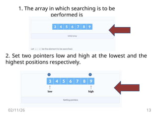
1. The arrayin which searching is to be
performed is
2. Set two pointers low and high at the lowest and the
highest positions respectively.
02/11/26 13
02/11/26 17
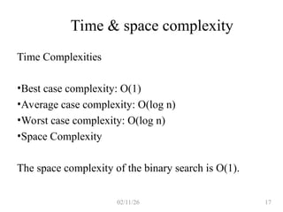
Time &space complexity
Time Complexities
•Best case complexity: O(1)
•Average case complexity: O(log n)
•Worst case complexity: O(log n)
•Space Complexity
The space complexity of the binary search is O(1).
18.
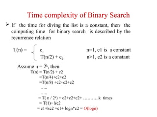
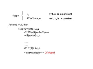
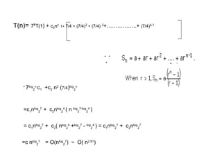
Time complexity ofBinary Search
If the time for diving the list is a constant, then the
computing time for binary search is described by the
recurrence relation
T(n) = c1 n=1, c1 is a constant
T(n/2) + c2 n>1, c2 is a constant
T(n) = T(n/2) + c2
=T(n/4)+c2+c2
=T(n/8) +c2+c2+c2
…..
…..
= T( n / 2k
) + c2+c2+c2+ ………..k times
= T(1)+ kc2
= c1+kc2 =c1+ logn*c2 = O(logn)
Assume n = 2k
, then
19.
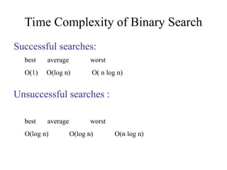
Time Complexity ofBinary Search
Successful searches:
best average worst
O(1) O(log n) O( n log n)
Unsuccessful searches :
best average worst
O(log n) O(log n) O(n log n)
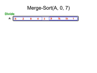
20.
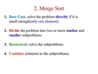
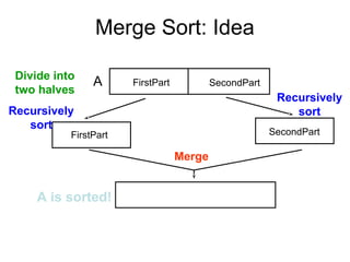
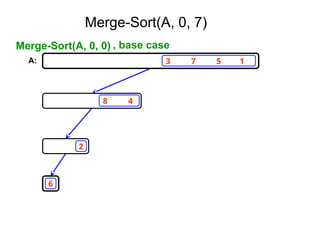
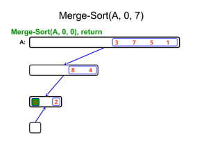
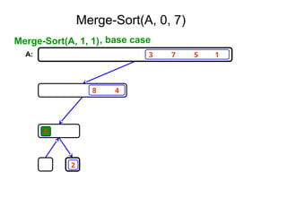
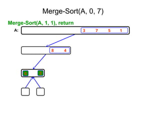
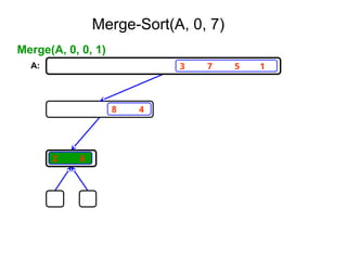
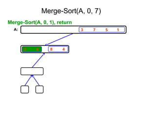
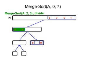
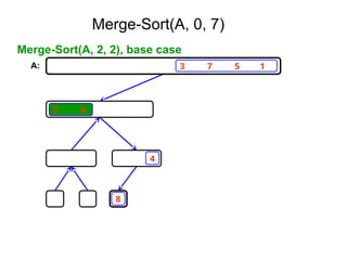
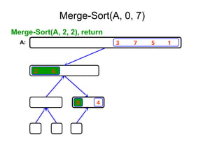
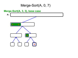
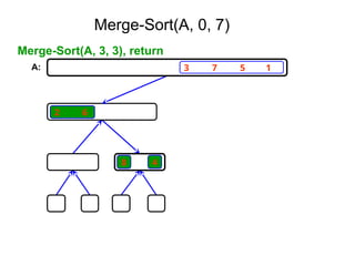
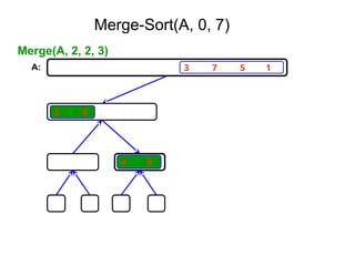
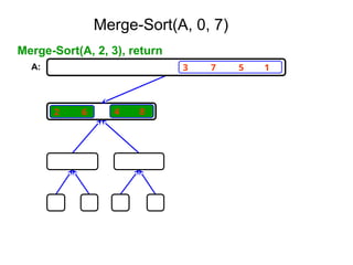
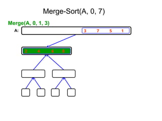
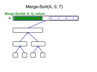
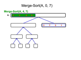
2. Merge Sort
1.Base Case, solve the problem directly if it is
small enough(only one element).
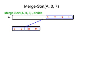
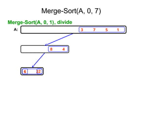
2. Divide the problem into two or more similar and
smaller subproblems.
3. Recursively solve the subproblems.
4. Combine solutions to the subproblems.
Merge Sort: Algorithm
MergeSort( low,high)
// sorts the elements a[low],…,a[high] which are in the global array
//a[1:n] into ascending order ( increasing order ).
// Small(p) is true if there is only one element to sort. In this case the list is
// already sorted.
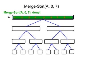
{ if ( low<high ) then // if there are more than one element
{
mid ← (low+high)/2;
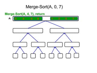
MergeSort(low,mid);
MergeSort(mid+1, high);
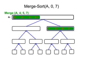
Merge(low, mid, high);
}
Recursive Calls
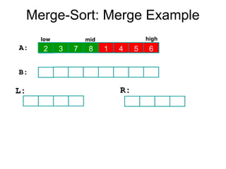
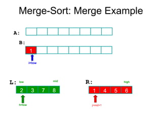
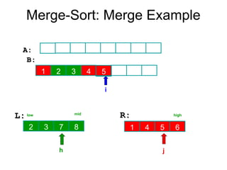
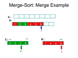
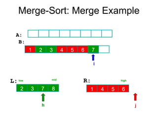
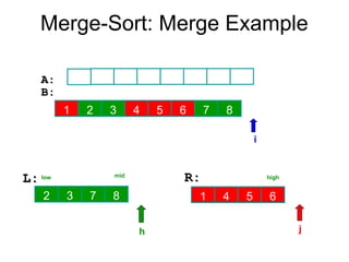
Algorithm Merge(low,mid,high)
// a[low:high]is a global array containing two sorted subsets in a[low:mid]
// and in a[mid+1:high]. The goal is to merge these two sets into a single
// set residing in a [low:high]. b[ ] is a temporary global array.
{
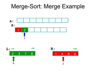
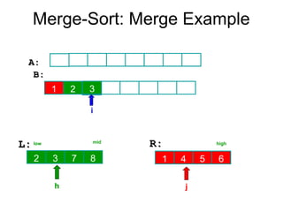
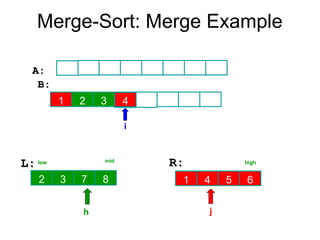
h:=low; j:=mid+1; i:=low;
while( h ≤ mid ) and ( j ≤ high ) do
{
if( a[h] ≤ a[j] ) then
{
b[i]:=a[h]; h:=h+1;
}
else
{
b[i]:=a[j]; j:=j+1;
}
i:=i+1;
}
58.
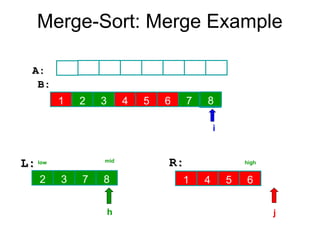
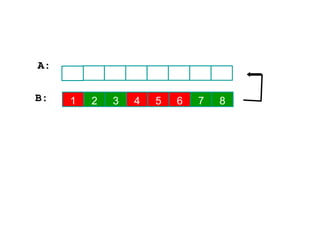
if( h >mid ) then
for k:=j to high do
{
b[i] := a[k]; i:= i+1;
}
else
for k:=h to mid do
{
b[i] := a[k]; i:= i+1;
}
for k:= low to high do a[k]:=b[k];
}
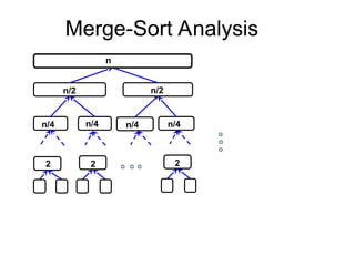
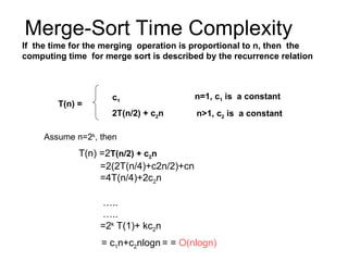
Merge-Sort Time Complexity
Ifthe time for the merging operation is proportional to n, then the
computing time for merge sort is described by the recurrence relation
n>1, c2 is a constant
n=1, c1 is a constant
2T(n/2) + c2n
c1
T(n) =
Assume n=2k
, then
T(n) =2T(n/2) + c2n
=2(2T(n/4)+c2n/2)+cn
=4T(n/4)+2c2n
…..
…..
=2k
T(1)+ kc2n
= c1n+c2nlogn = = O(nlogn)
61.
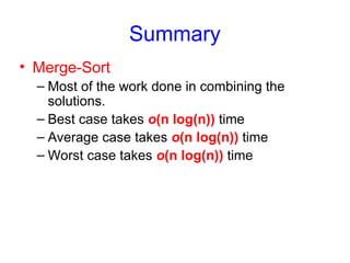
Summary
• Merge-Sort
– Mostof the work done in combining the
solutions.
– Best case takes o(n log(n)) time
– Average case takes o(n log(n)) time
– Worst case takes o(n log(n)) time
62.
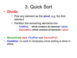
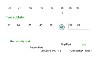
3. Quick Sort
•Divide:
• Pick any element as the pivot, e.g, the first
element
• Partition the remaining elements into
FirstPart, which contains all elements < pivot
SecondPart, which contains all elements > pivot
• Recursively sort FirstPart and SecondPart.
• Combine: no work is necessary since sorting is done in
place.
63.
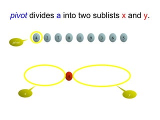
pivot divides ainto two sublists x and y.
4 2 7 8 1 9 3 6 5
4
pivot
4 2 7 8 1 9 3 6 5
x y
Keep going fromleft side as long as a[ i ]<pivot and from the right
side as long as a[ j ]>pivot
85 24 63 95 17 31 45 98
i j
85 24 63 95 17 31 45 98
85 24 63 95 17 31 45 98
85 24 63 95 17 31 45 98
i
i
i
j
j
j
Process:
pivot
66.
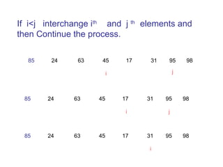
If i<j interchangeith
and j th
elements and
then Continue the process.
85 24 63 45 17 31 95 98
i j
85 24 63 45 17 31 95 98
i j
85 24 63 45 17 31 95 98
i
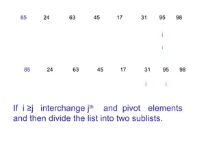
67.
85 24 6345 17 31 95 98
i
j
85 24 63 45 17 31 95 98
j
If i ≥j interchange jth
and pivot elements
and then divide the list into two sublists.
i
Quick Sort Algorithm:
Algorithm QuickSort(low,high)
//Sorts the elements a[low],…..,a[high] which resides
//in the global array a[1:n] into ascending order;
// a[n+1] is considered to be defined and must ≥ all the
// elements in a[1:n].
{
if( low< high ) // if there are more than one element
{ // divide p into two subproblems.
j :=Partition(low,high);
// j is the position of the partitioning element.
QuickSort(low,j-1);
QuickSort(j+1,high);
// There is no need for combining solutions.
}
}
70.
Algorithm Partition(low, high)
{
pivot:=a[ low ] ; i:=low; j:= high+1;
while( i < j ) do
{
i++;
while( a[ i ] < pivot ) do
i++;
j--;
while( a[ j ] > pivot ) do
j--;
if ( i < j ) then Interchange(i, j ); // interchange ith
and
} // jth
elements.
Interchange(low, j ); return j; // interchange pivot and jth
element.
}
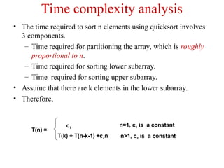
Time complexity analysis
•The time required to sort n elements using quicksort involves
3 components.
– Time required for partitioning the array, which is roughly
proportional to n.
– Time required for sorting lower subarray.
– Time required for sorting upper subarray.
• Assume that there are k elements in the lower subarray.
• Therefore,
n>1, c2 is a constant
n=1, c1 is a constant
T(k) + T(n-k-1) +c2n
c1
T(n) =
73.
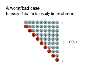
A worst/bad case
Itoccurs if the list is already in sorted order
8
7
6
5
4
3
2
1
1 2 3 4 5 6 7 8
2 3 4 5 6 7 8
3 4 5 6 7 8
4 5 6 7 8
5 6 7 8
6 7 8
7 8
8
O(n2
)
9
9
9
9
9
9
9
9
9
9
contd...
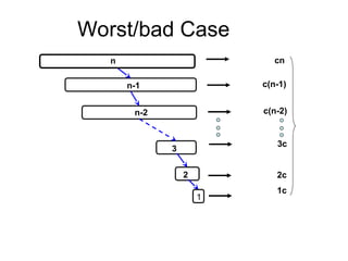
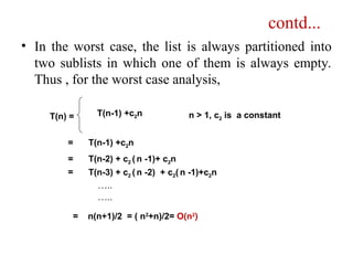
• In theworst case, the list is always partitioned into
two sublists in which one of them is always empty.
Thus , for the worst case analysis,
T(n-1) +c2n
T(n) = n > 1, c2 is a constant
T(n-1) +c2n
=
T(n-2) + c2 ( n -1)+ c2n
=
= T(n-3) + c2 ( n -2) + c2( n -1)+c2n
…..
…..
= n(n+1)/2 = ( n2
+n)/2= O(n2
)
76.
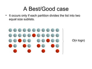
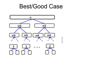
A Best/Good case
•It occurs only if each partition divides the list into two
equal size sublists.
O(n logn)
n>1, c2 isa constant
n=1, c1 is a constant
2T(n/2) + c2n
c1
T(n) =
Assume n=2k
, then
T(n) =2T(n/2) + c2n
=2(2T(n/4)+c2n/2)+cn
=4T(n/4)+2c2n
…..
…..
=2k
T(1)+ kc2n
= c1n+c2nlogn = = O(nlogn)
79.
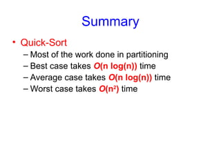
Summary
• Quick-Sort
– Mostof the work done in partitioning
– Best case takes O(n log(n)) time
– Average case takes O(n log(n)) time
– Worst case takes O(n2
) time
Basic Matrix Multiplication
voidmatrix_mult (){
for (i = 1; i <= n; i++) {
for (j = 1; j <= n; j++) {
for(k=1; k<=n; k++){
C[i,j]=C[i,j]+A[i,k]+B[k,j];
}
}}
Time complexity of above algorithm is
T(n)=O(n3
)
Let A an B two n×n matrices. The product C=AB is also an n×n matrix.
82.
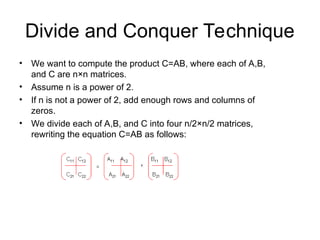
Divide and ConquerTechnique
• We want to compute the product C=AB, where each of A,B,
and C are n×n matrices.
• Assume n is a power of 2.
• If n is not a power of 2, add enough rows and columns of
zeros.
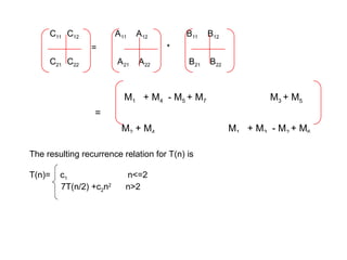
• We divide each of A,B, and C into four n/2×n/2 matrices,
rewriting the equation C=AB as follows:
83.
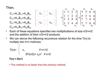
Then,
C11=A11B11+A12B21
C12=A11B12+A12B22
C21=A21B11+A22B21
C22=A21B12+A22B22
• Each ofthese equations specifies two multiplications of size n/2×n/2
and the addition of their n/2×n/2 products.
• We can derive the following recurrence relation for the time T(n) to
multiply two n×n matrices:
T(n)= c1 if n<=2
8T(n/2)+ c2n2
if n>2
T(n) = O(n3
)
• This method is no faster than the ordinary method.
8
8
8
8
7
7
7
7
6
6
6
6
5
5
5
5
4
4
4
4
3
3
3
3
2
2
2
2
1
1
1
1
22
21
12
11
C
C
C
C
C
c11 c12
c22
c21
A11 A12
A21 A22 B21 B22
B11 B12
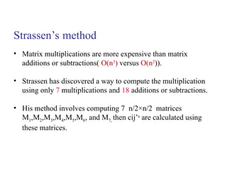
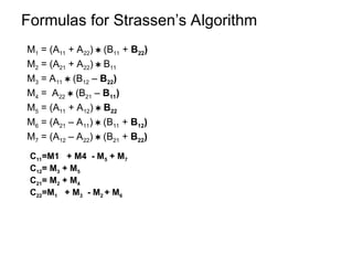
Strassen’s method
• Matrixmultiplications are more expensive than matrix
additions or subtractions( O(n3
) versus O(n2
)).
• Strassen has discovered a way to compute the multiplication
using only 7 multiplications and 18 additions or subtractions.
• His method involves computing 7 n/2×n/2 matrices
M1,M2,M3,M4,M5,M6, and M7, then cij’s
are calculated using
these matrices.
#21 Divide: if the initial array A has at least two elements (nothing needs to be done if A has zero or one elements), divide A into two subarrays each containing about half of the elements of A.
Conquer: sort the two subarrays using Merge Sort.
Combine: merging the two sorted subarray into one sorted array
#61 no specific input triggers worst-case behavior
the worst-case is only determined by the output of the random-number generator
Disadvantage:
Unstable in running time
Finding “pivot” element is a big issue!
#79 no specific input triggers worst-case behavior
the worst-case is only determined by the output of the random-number generator
Disadvantage:
Unstable in running time
Finding “pivot” element is a big issue!


![Iterative Method
Algorithm BinSearch(a, n, x)
// a is an array of size n, x is the key element to be searched.
{ low:=1; high:=n;
while( low ≤ high)
{
mid:=(low+high)/2;
if( x < a[mid] ) then high := mid-1;
else if( x > a[mid] ) then low := mid+1;
else return mid;
}
return 0;
}](https://image.slidesharecdn.com/daa-unit-ii-260211045705-50149743/85/Divide-and-Conquer-Strategy-and-their-performance-analysis-in-DAA-10-320.jpg)
![Recursive Algorithm ( Divide and Conquer Technique)
Algorithm BinSrch (a, low, high, x)
//Given an array a [ low : high ]of elements in increasing
//order,1≤low≤high,determine whether x is present, and
//if so, return j such that x=a[j]; else return 0.
{
if( low = high ) then // If small(P)
{
if( x=a[low] ) then return low;
else return 0;
}
else](https://image.slidesharecdn.com/daa-unit-ii-260211045705-50149743/85/Divide-and-Conquer-Strategy-and-their-performance-analysis-in-DAA-11-320.jpg)
![{
//Reduce p into a smaller subproblem.
mid:= (low+high)/2
if( x = a[mid] ) then return mid;
else if ( x<a[mid] ) then
return BinSrch(a, low, mid-1, x);
else
return BinSrch(a, mid+1, high, x);
}
}](https://image.slidesharecdn.com/daa-unit-ii-260211045705-50149743/85/Divide-and-Conquer-Strategy-and-their-performance-analysis-in-DAA-12-320.jpg)
![Ex:- [ 179, 254, 285, 310, 351, 423, 450, 520,
652,861 ]
Tree of calls of merge sort
1,10
1,5 6,10
1,3 4,5 6,8 9,10
1,2 3,3 4,4 5,5 6,7 8,8 9,9 10,10
1,1 2,2 6,6 7,7](https://image.slidesharecdn.com/daa-unit-ii-260211045705-50149743/85/Divide-and-Conquer-Strategy-and-their-performance-analysis-in-DAA-44-320.jpg)
![Merge Sort: Algorithm
MergeSort ( low,high)
// sorts the elements a[low],…,a[high] which are in the global array
//a[1:n] into ascending order ( increasing order ).
// Small(p) is true if there is only one element to sort. In this case the list is
// already sorted.
{ if ( low<high ) then // if there are more than one element
{
mid ← (low+high)/2;
MergeSort(low,mid);
MergeSort(mid+1, high);
Merge(low, mid, high);
}
Recursive Calls](https://image.slidesharecdn.com/daa-unit-ii-260211045705-50149743/85/Divide-and-Conquer-Strategy-and-their-performance-analysis-in-DAA-45-320.jpg)
![Algorithm Merge(low,mid,high)
// a[low:high] is a global array containing two sorted subsets in a[low:mid]
// and in a[mid+1:high]. The goal is to merge these two sets into a single
// set residing in a [low:high]. b[ ] is a temporary global array.
{
h:=low; j:=mid+1; i:=low;
while( h ≤ mid ) and ( j ≤ high ) do
{
if( a[h] ≤ a[j] ) then
{
b[i]:=a[h]; h:=h+1;
}
else
{
b[i]:=a[j]; j:=j+1;
}
i:=i+1;
}](https://image.slidesharecdn.com/daa-unit-ii-260211045705-50149743/85/Divide-and-Conquer-Strategy-and-their-performance-analysis-in-DAA-57-320.jpg)
![if( h > mid ) then
for k:=j to high do
{
b[i] := a[k]; i:= i+1;
}
else
for k:=h to mid do
{
b[i] := a[k]; i:= i+1;
}
for k:= low to high do a[k]:=b[k];
}](https://image.slidesharecdn.com/daa-unit-ii-260211045705-50149743/85/Divide-and-Conquer-Strategy-and-their-performance-analysis-in-DAA-58-320.jpg)
![Keep going from left side as long as a[ i ]<pivot and from the right
side as long as a[ j ]>pivot
85 24 63 95 17 31 45 98
i j
85 24 63 95 17 31 45 98
85 24 63 95 17 31 45 98
85 24 63 95 17 31 45 98
i
i
i
j
j
j
Process:
pivot](https://image.slidesharecdn.com/daa-unit-ii-260211045705-50149743/85/Divide-and-Conquer-Strategy-and-their-performance-analysis-in-DAA-65-320.jpg)
![Quick Sort Algorithm :
Algorithm QuickSort(low,high)
//Sorts the elements a[low],…..,a[high] which resides
//in the global array a[1:n] into ascending order;
// a[n+1] is considered to be defined and must ≥ all the
// elements in a[1:n].
{
if( low< high ) // if there are more than one element
{ // divide p into two subproblems.
j :=Partition(low,high);
// j is the position of the partitioning element.
QuickSort(low,j-1);
QuickSort(j+1,high);
// There is no need for combining solutions.
}
}](https://image.slidesharecdn.com/daa-unit-ii-260211045705-50149743/85/Divide-and-Conquer-Strategy-and-their-performance-analysis-in-DAA-69-320.jpg)
![Algorithm Partition(low, high)
{
pivot:= a[ low ] ; i:=low; j:= high+1;
while( i < j ) do
{
i++;
while( a[ i ] < pivot ) do
i++;
j--;
while( a[ j ] > pivot ) do
j--;
if ( i < j ) then Interchange(i, j ); // interchange ith
and
} // jth
elements.
Interchange(low, j ); return j; // interchange pivot and jth
element.
}](https://image.slidesharecdn.com/daa-unit-ii-260211045705-50149743/85/Divide-and-Conquer-Strategy-and-their-performance-analysis-in-DAA-70-320.jpg)
![Algorithm interchange (x,y )
{
temp=a[x];
a[x]=a[y];
a[y]=temp;
}](https://image.slidesharecdn.com/daa-unit-ii-260211045705-50149743/85/Divide-and-Conquer-Strategy-and-their-performance-analysis-in-DAA-71-320.jpg)
![Basic Matrix Multiplication
void matrix_mult (){
for (i = 1; i <= n; i++) {
for (j = 1; j <= n; j++) {
for(k=1; k<=n; k++){
C[i,j]=C[i,j]+A[i,k]+B[k,j];
}
}}
Time complexity of above algorithm is
T(n)=O(n3
)
Let A an B two n×n matrices. The product C=AB is also an n×n matrix.](https://image.slidesharecdn.com/daa-unit-ii-260211045705-50149743/85/Divide-and-Conquer-Strategy-and-their-performance-analysis-in-DAA-81-320.jpg)


![DSA[1]5655566666666666666666666666666.pptx](https://cdn.slidesharecdn.com/ss_thumbnails/dsa1-251221115013-1ff1f21a-thumbnail.jpg?width=640&height=640&fit=bounds)


