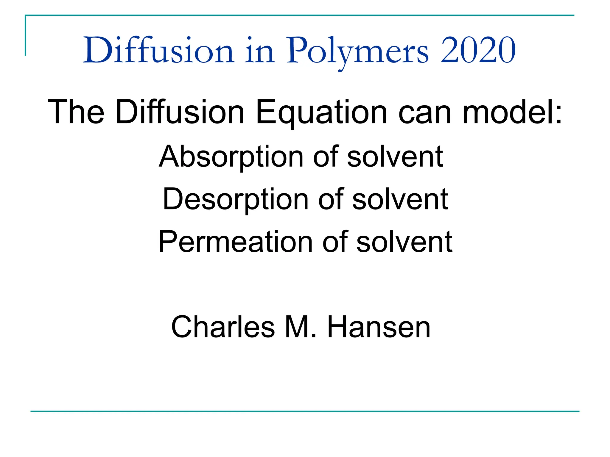
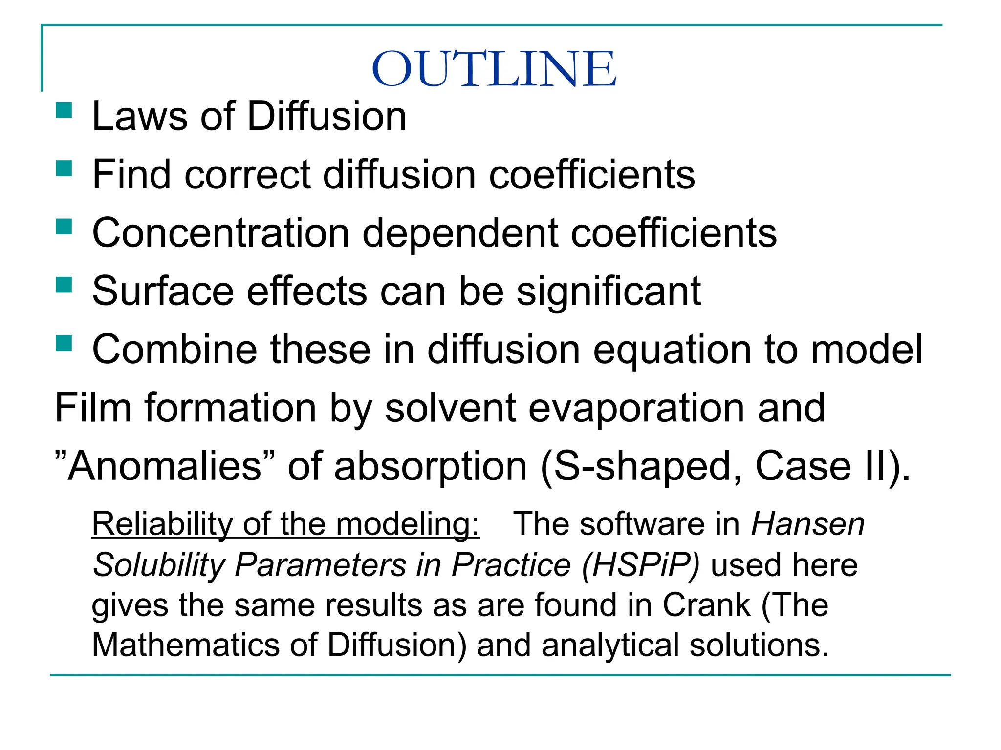
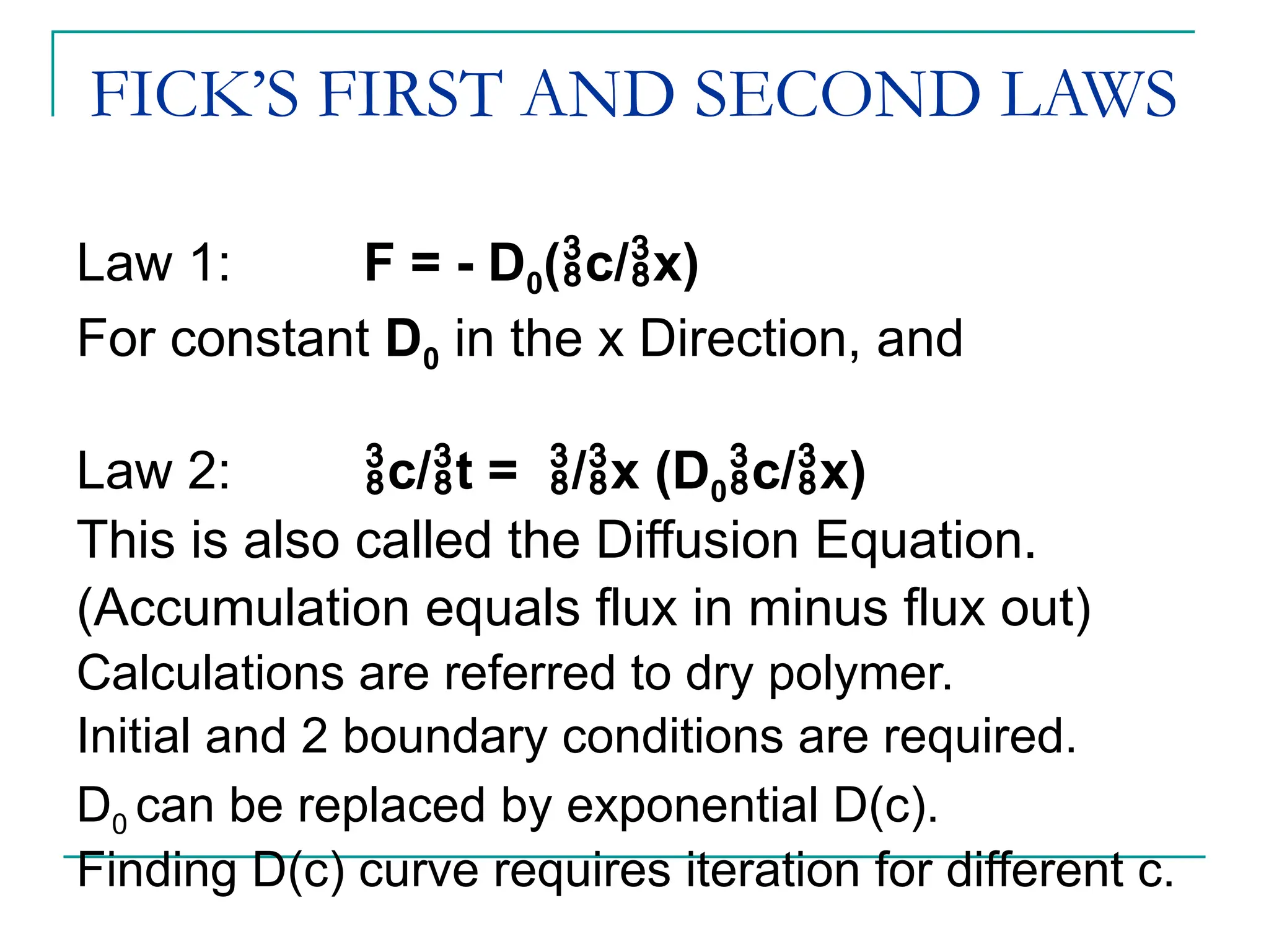
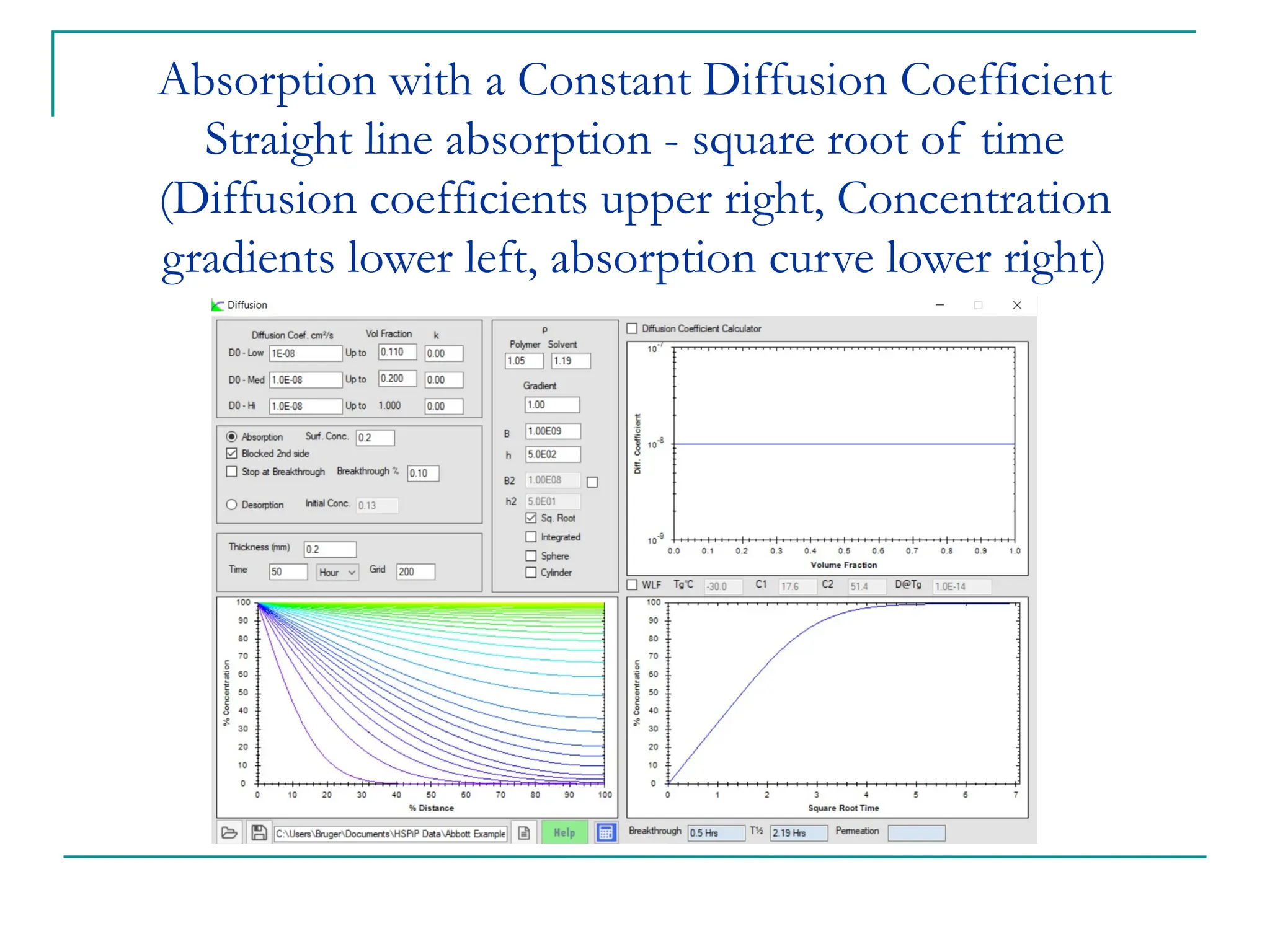
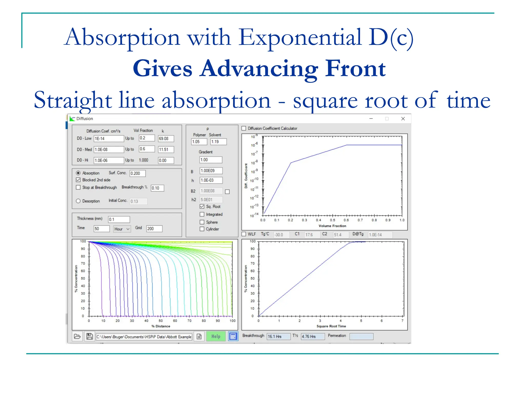
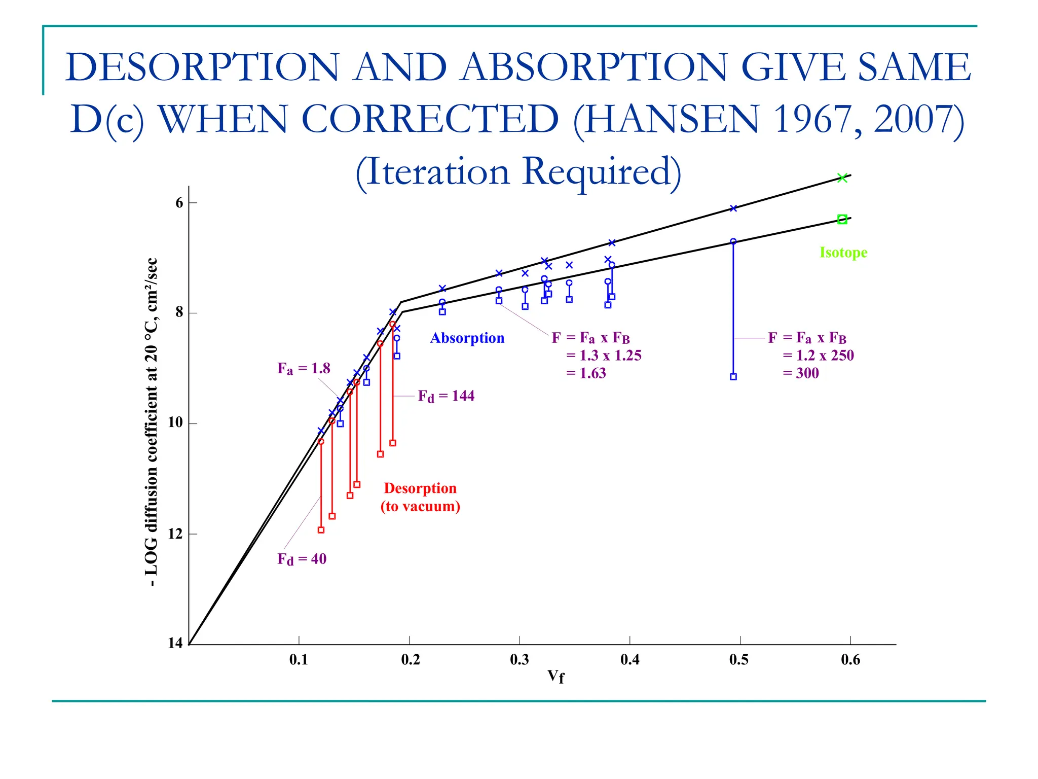
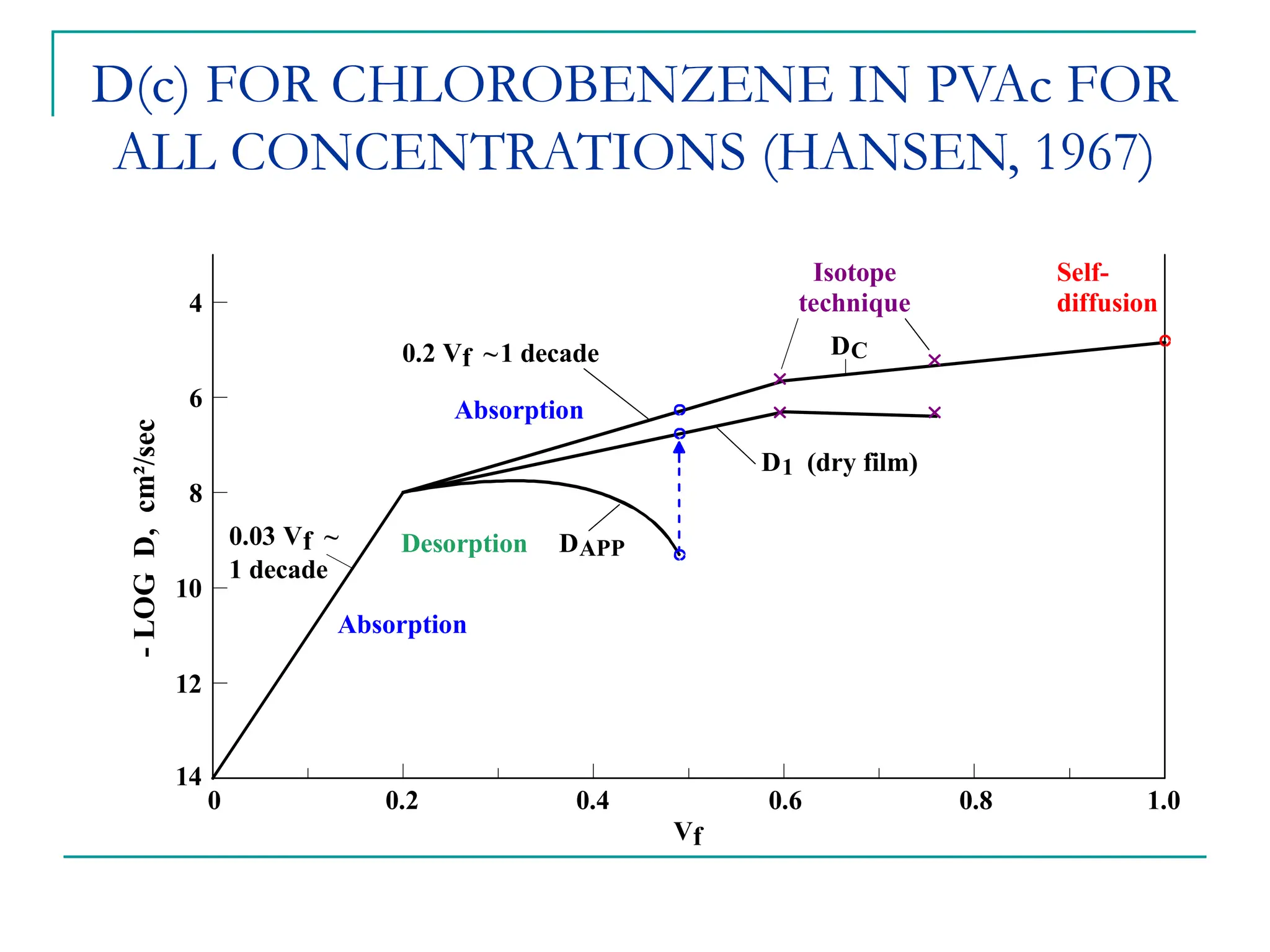
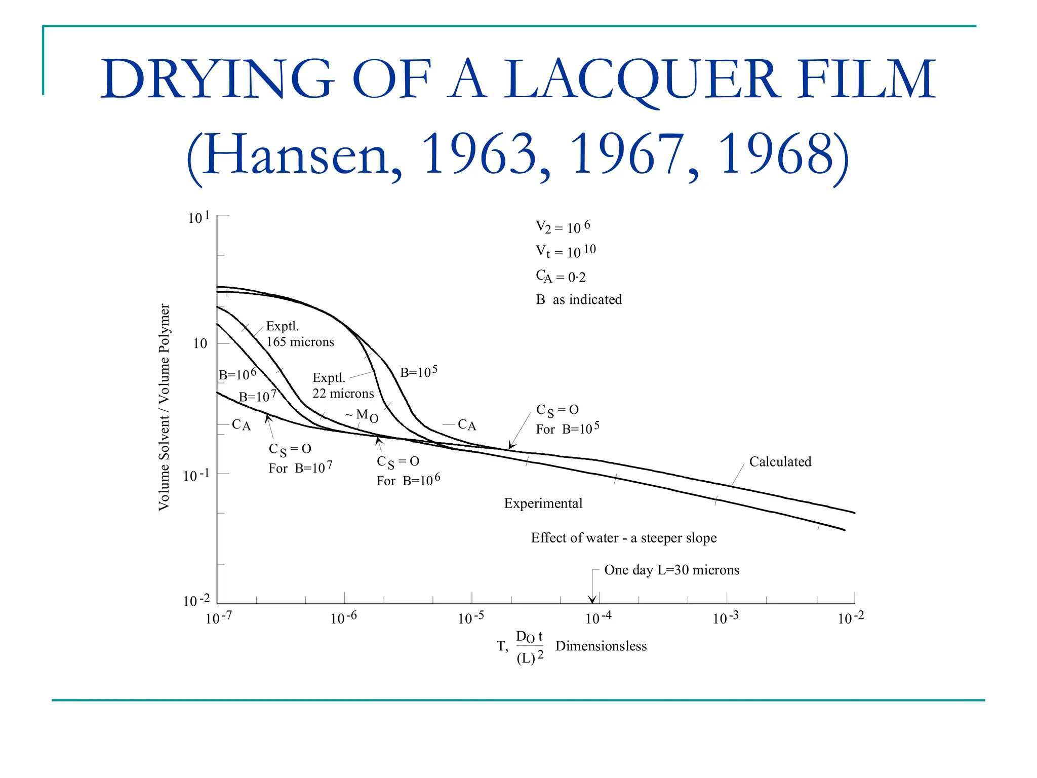
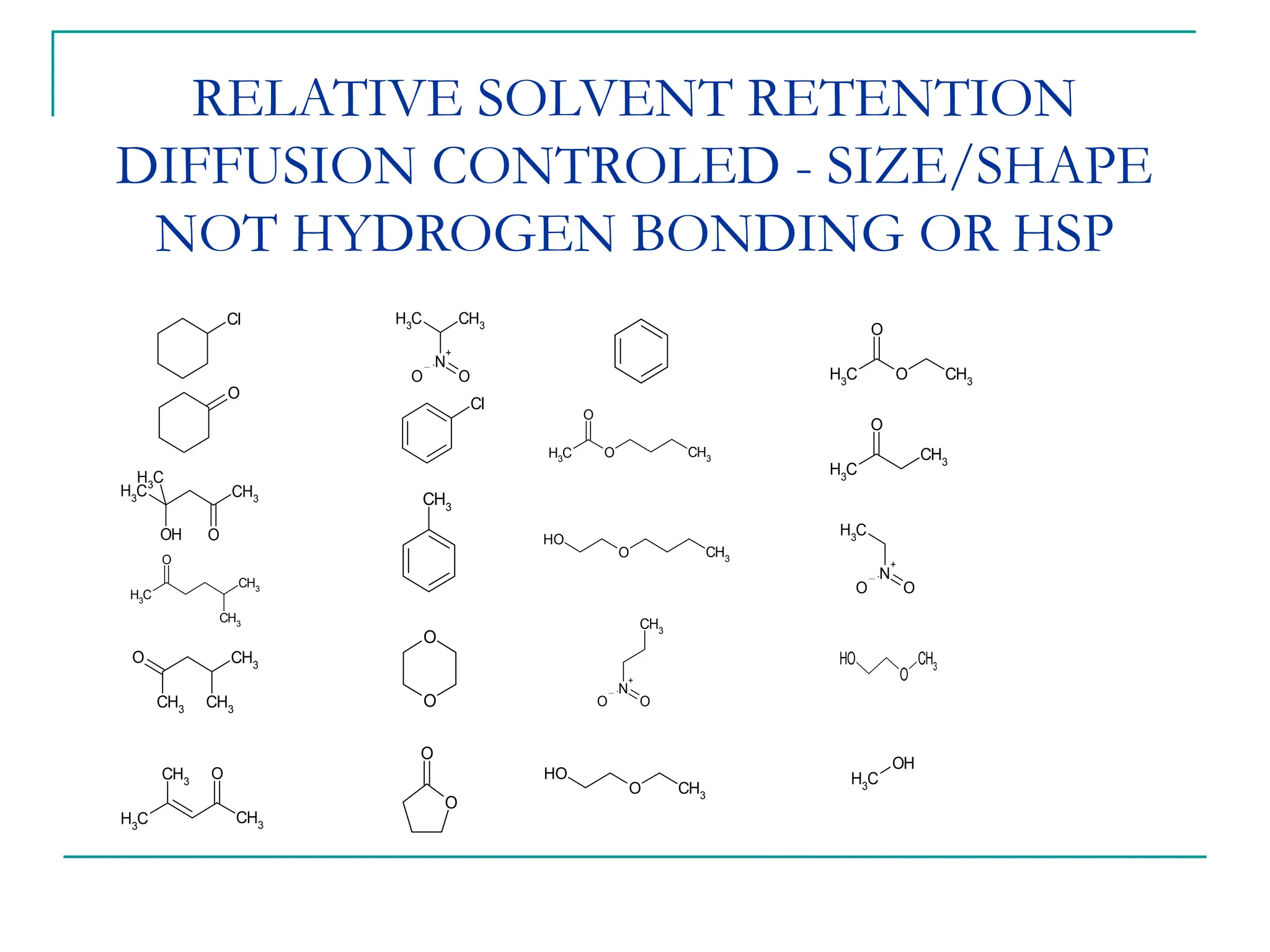
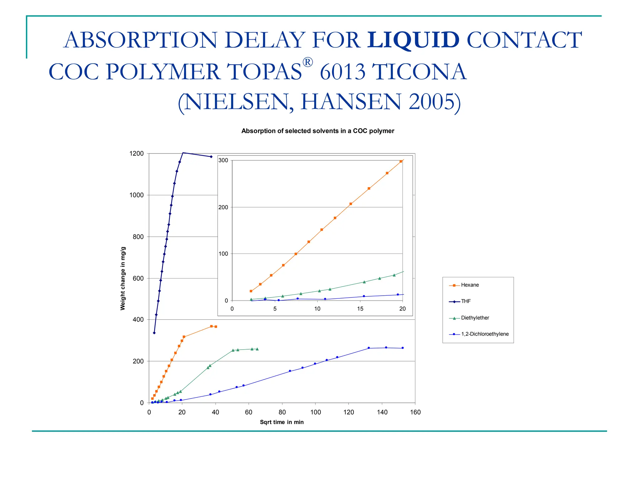
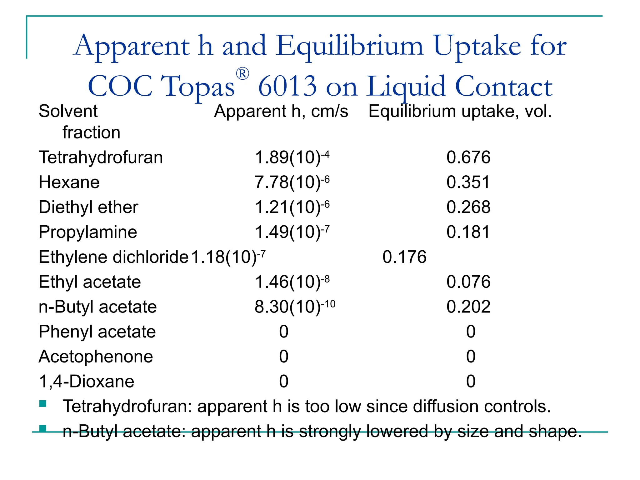
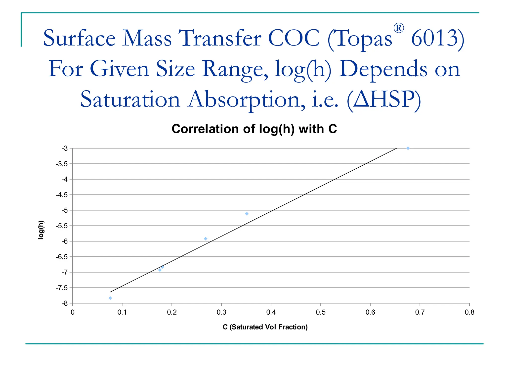
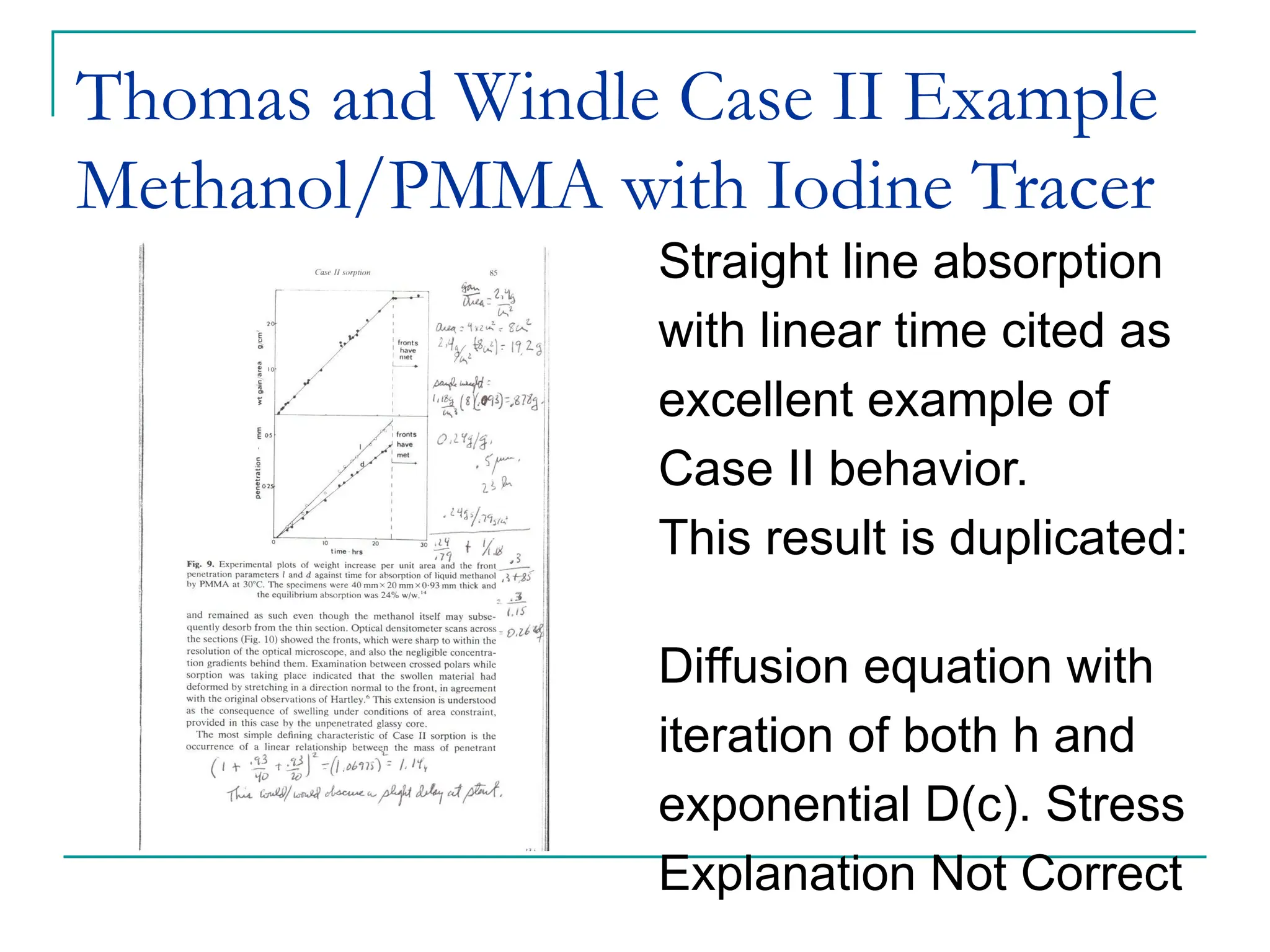
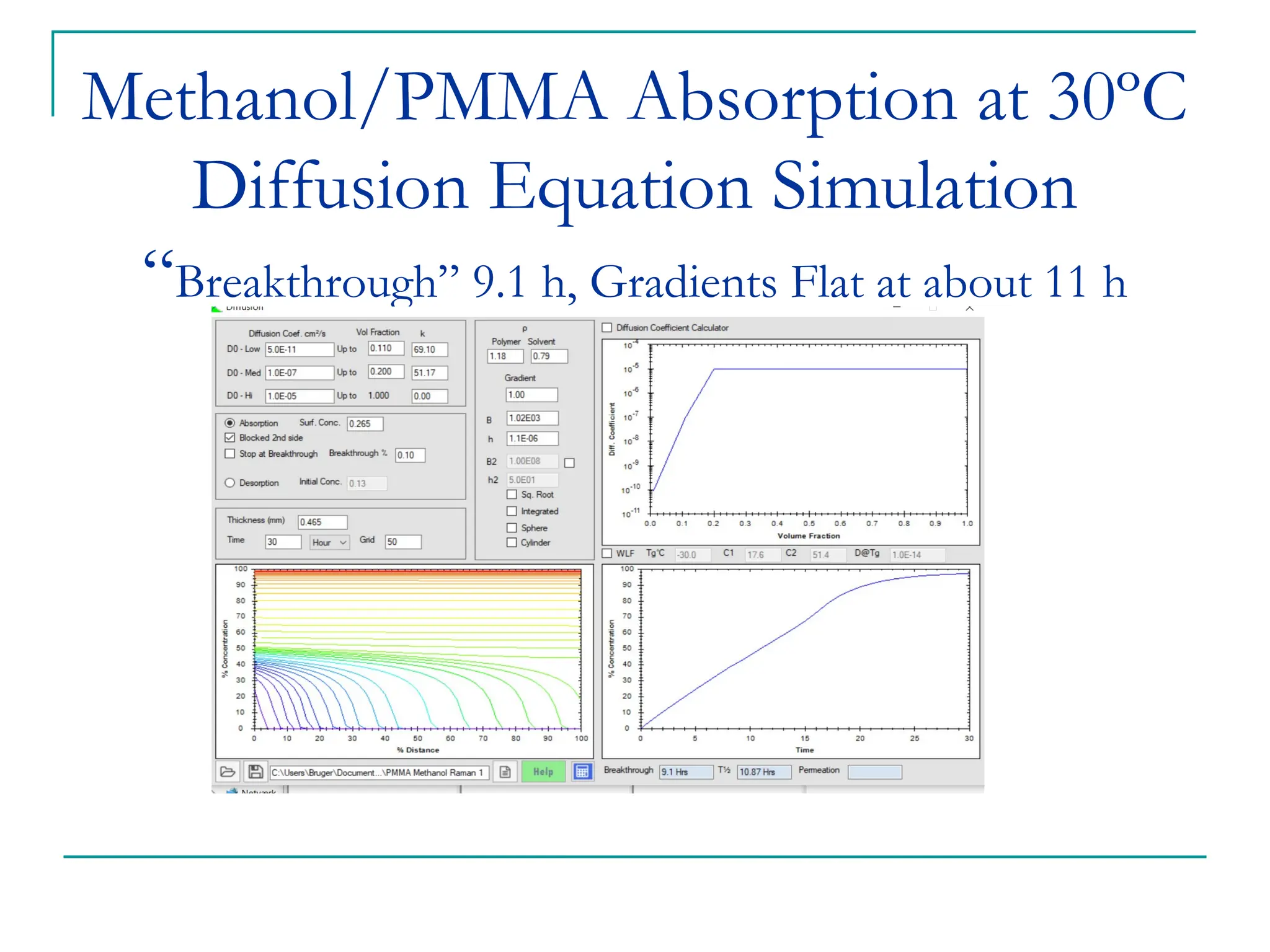
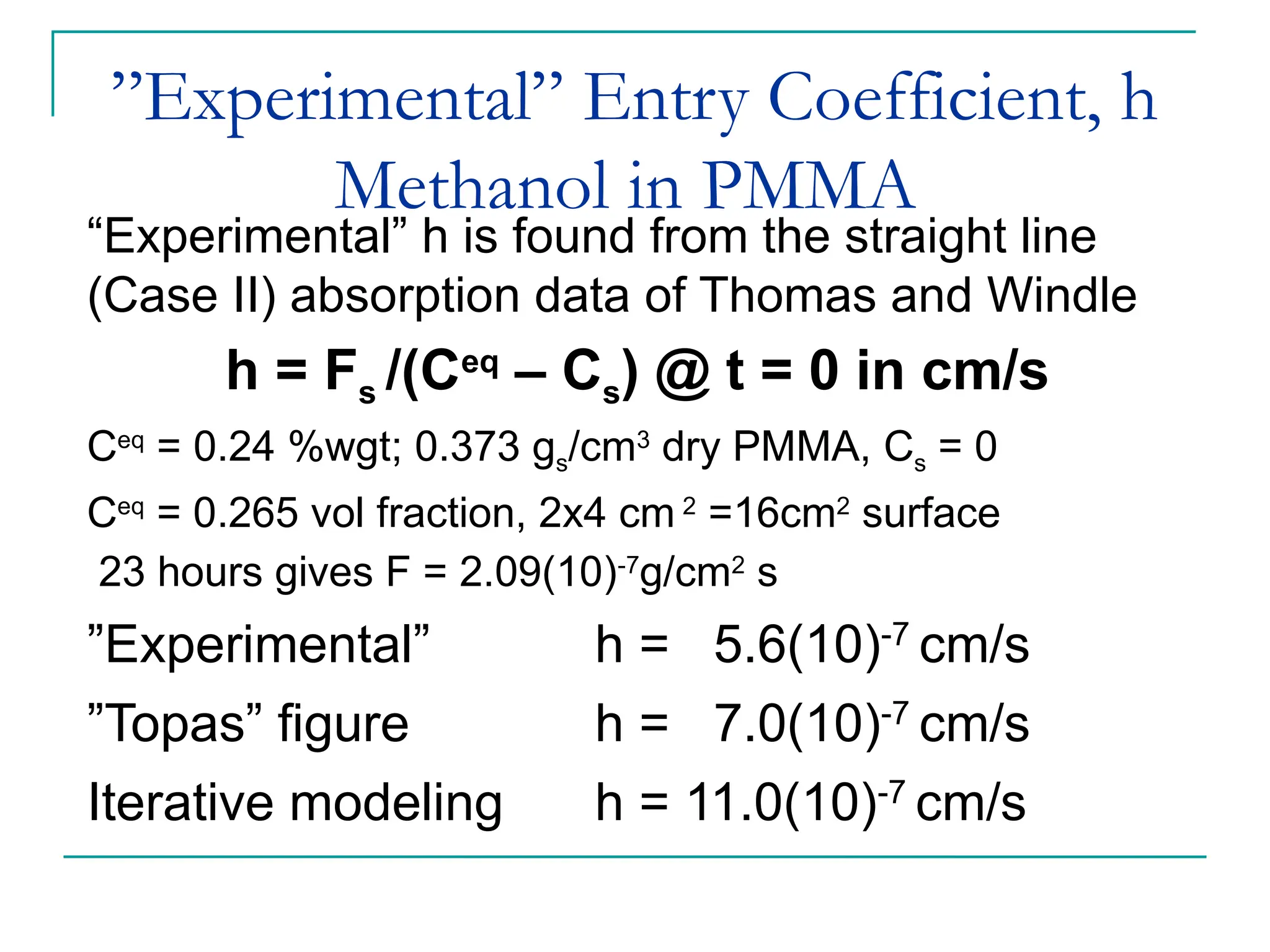
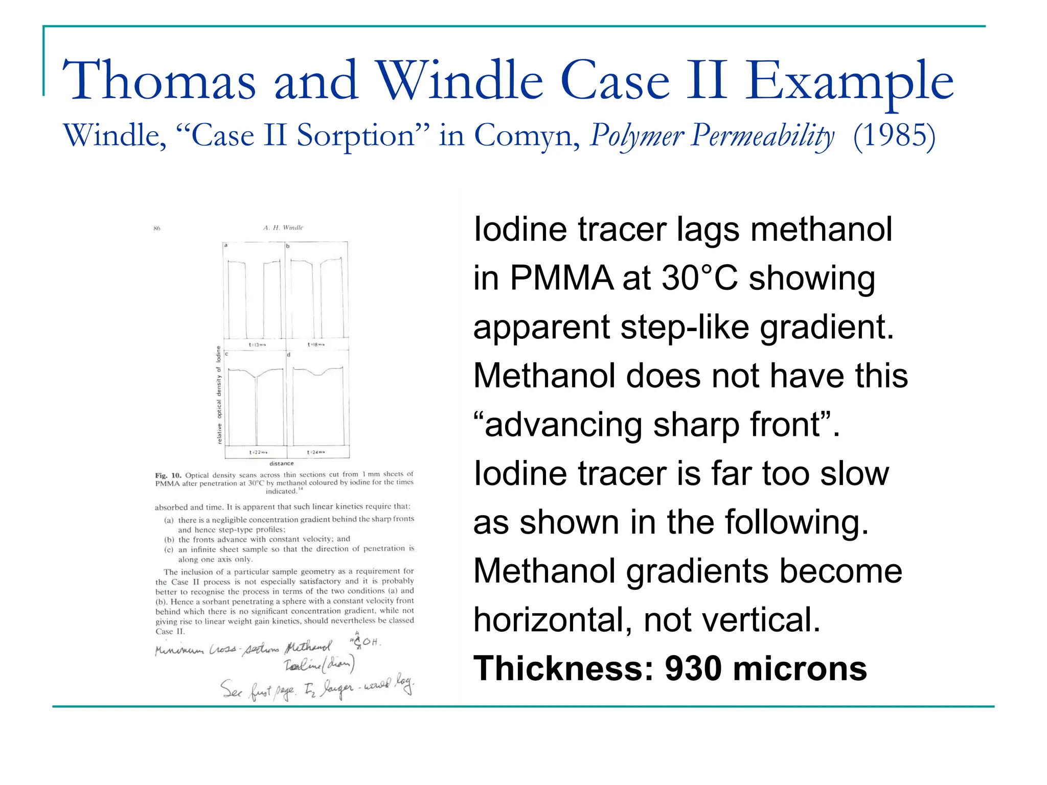
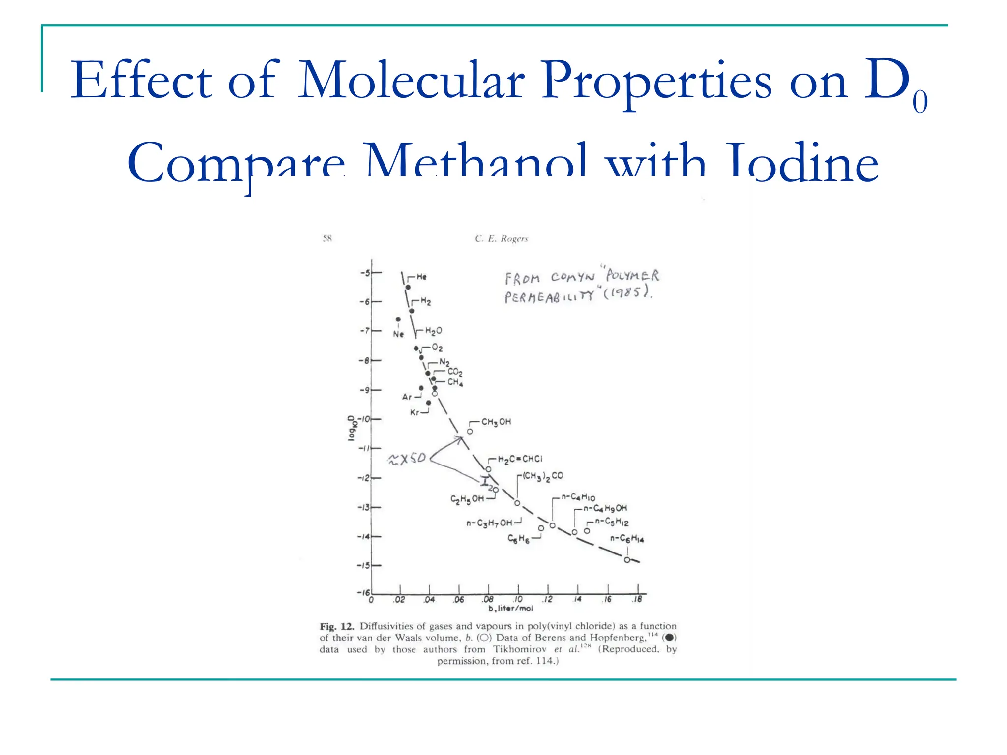
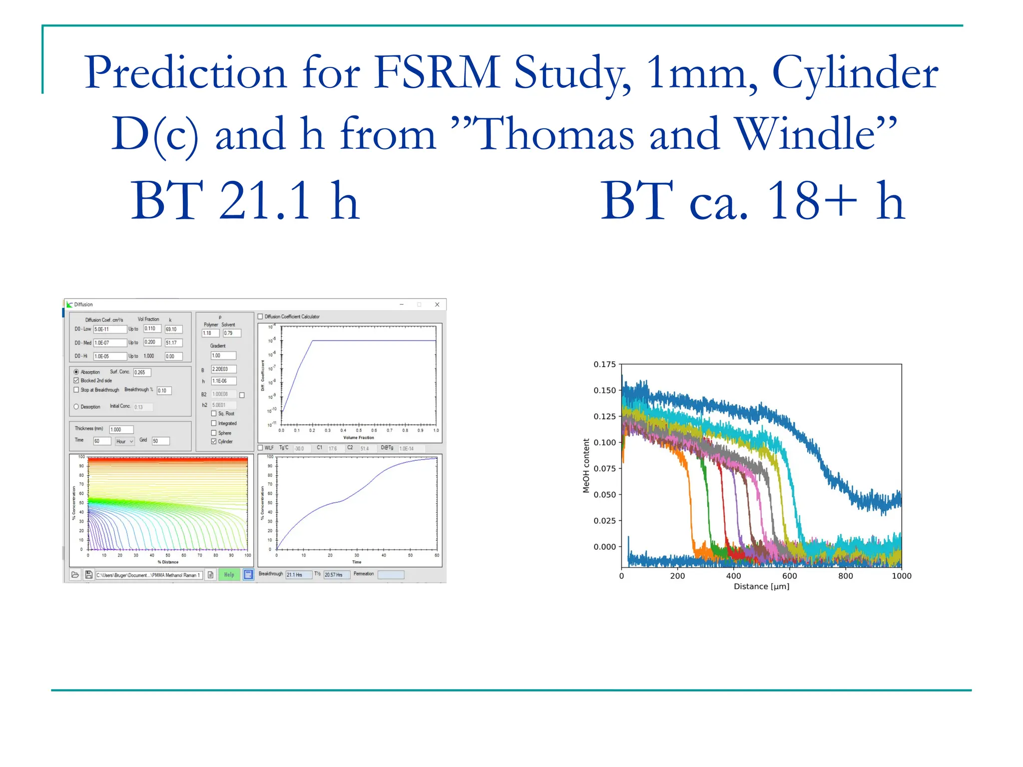
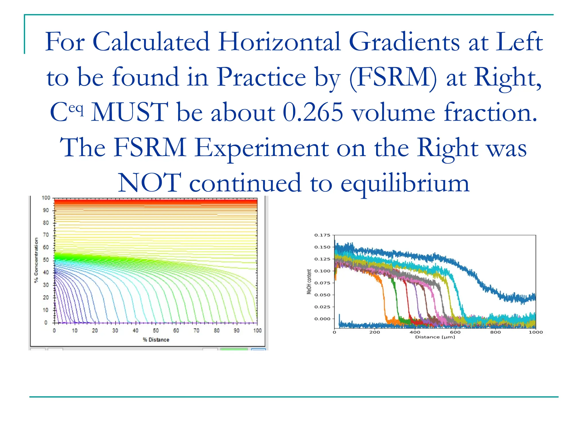
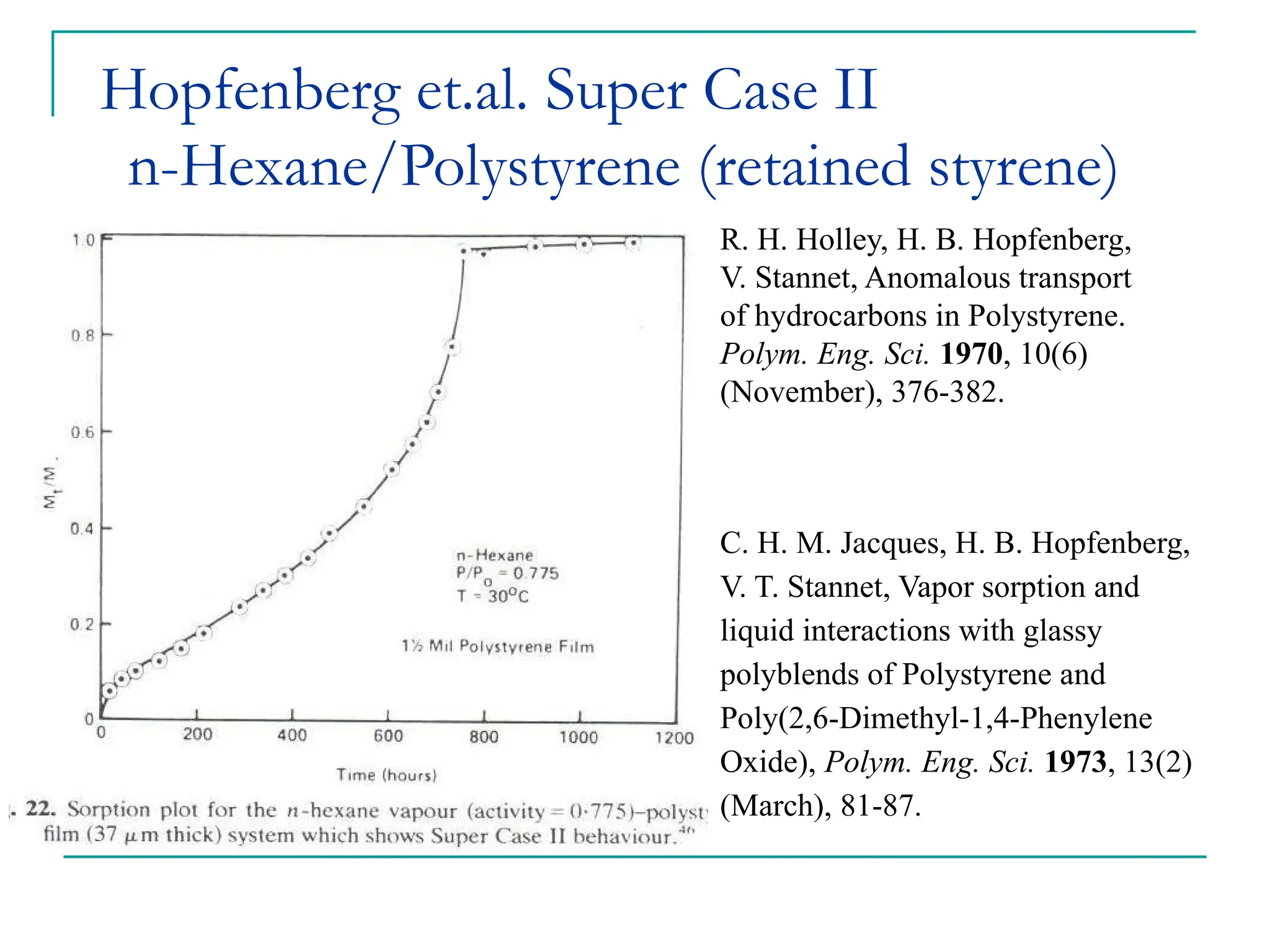
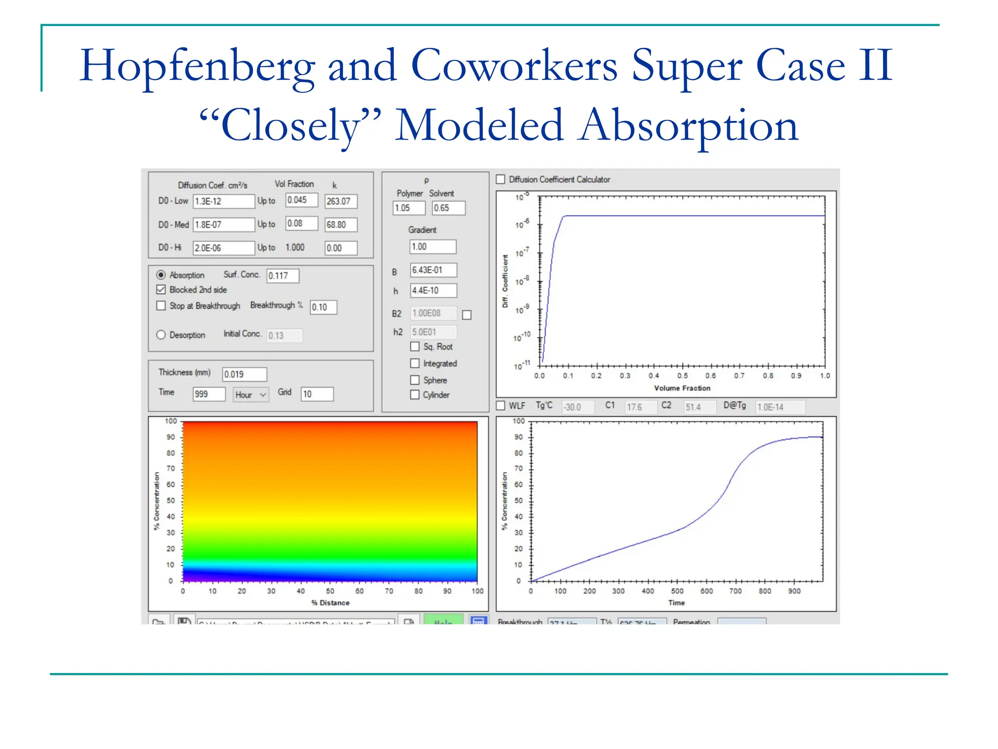
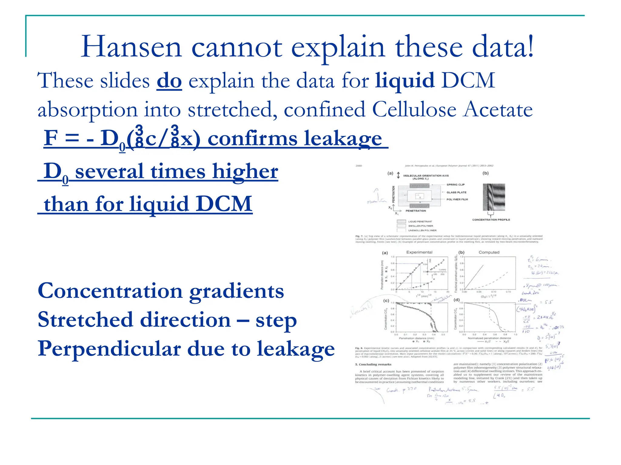
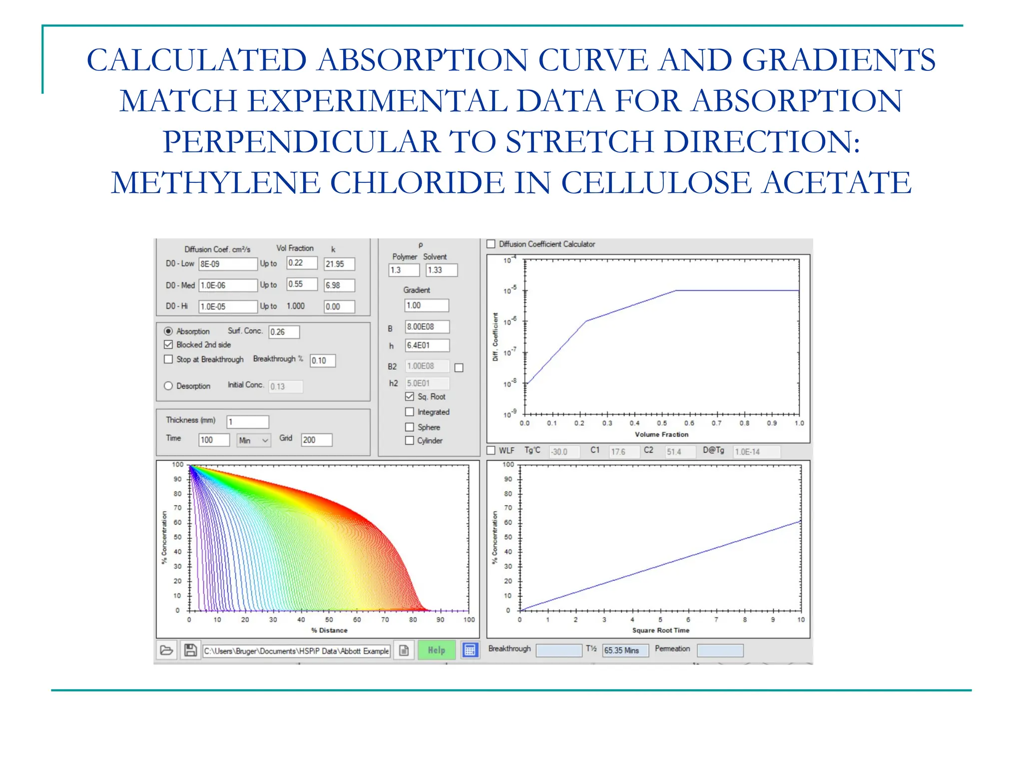
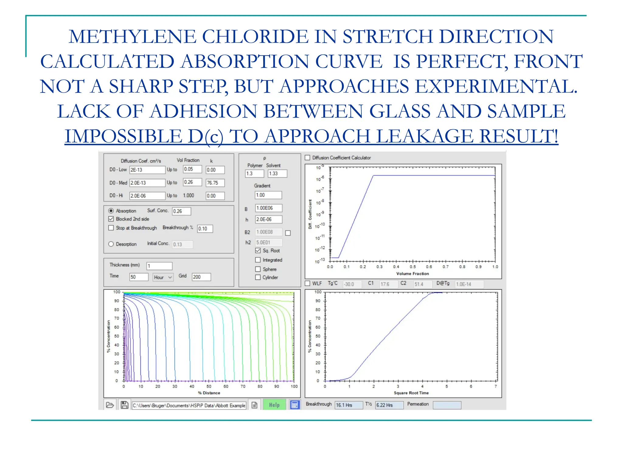
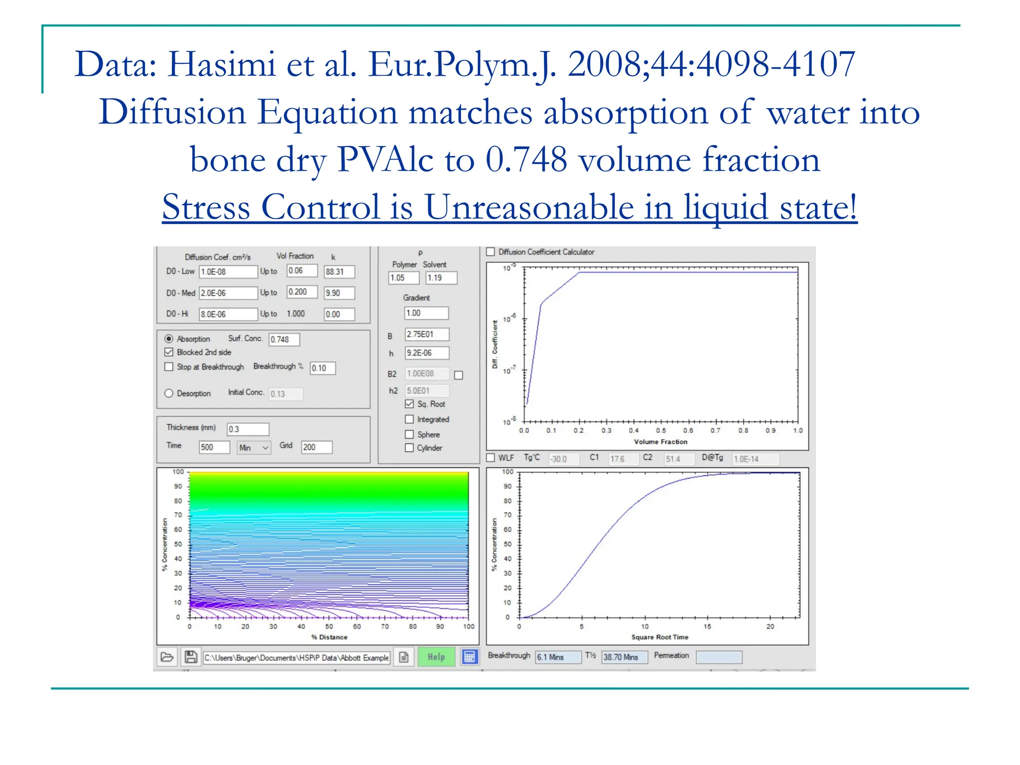
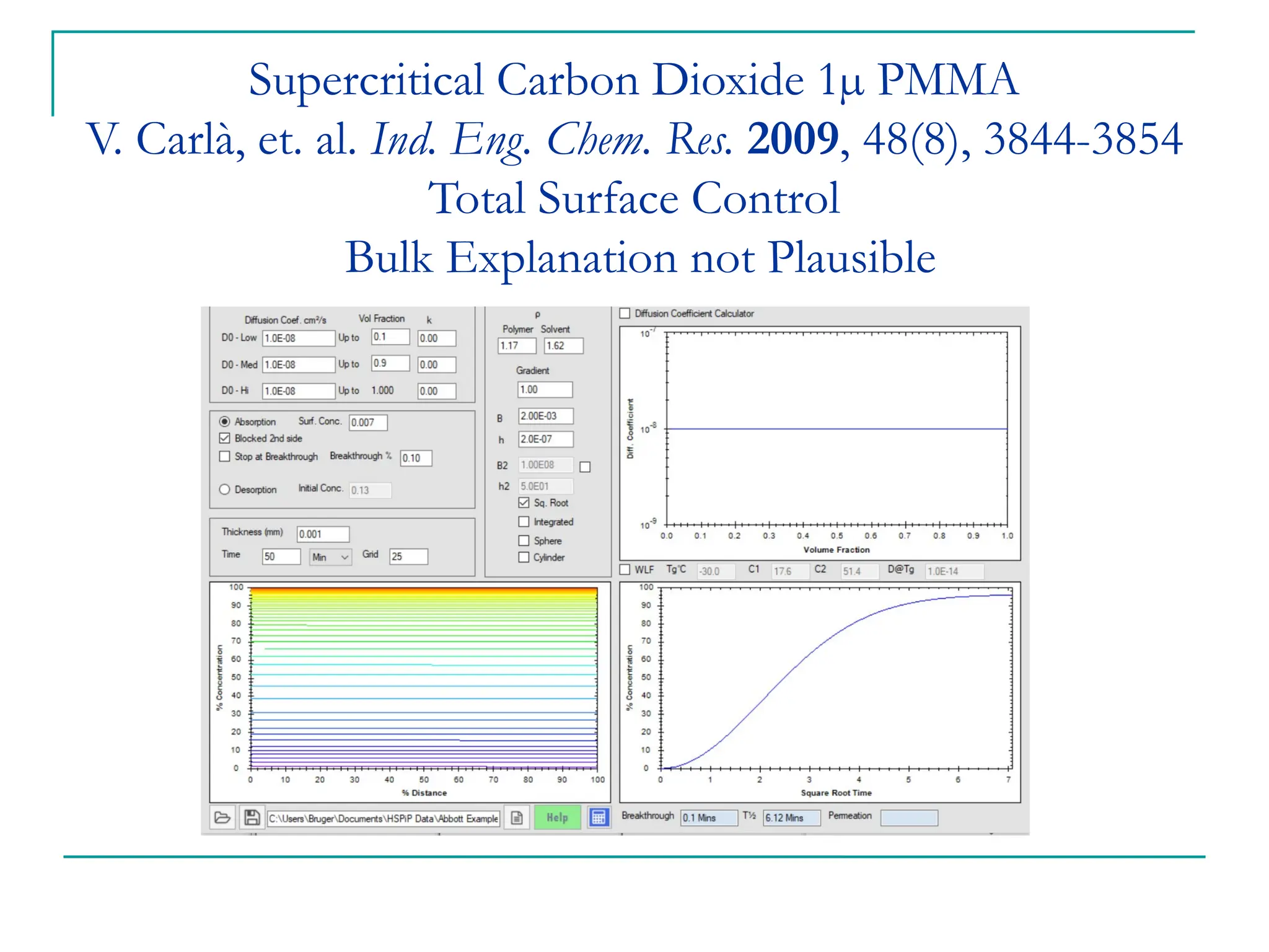
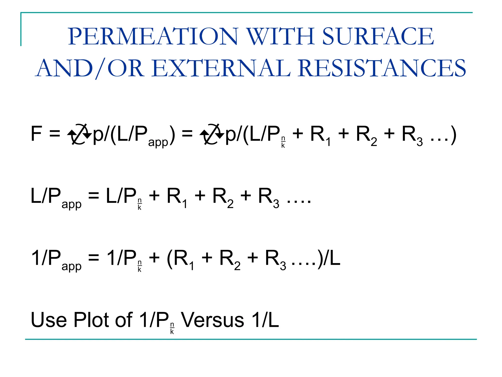
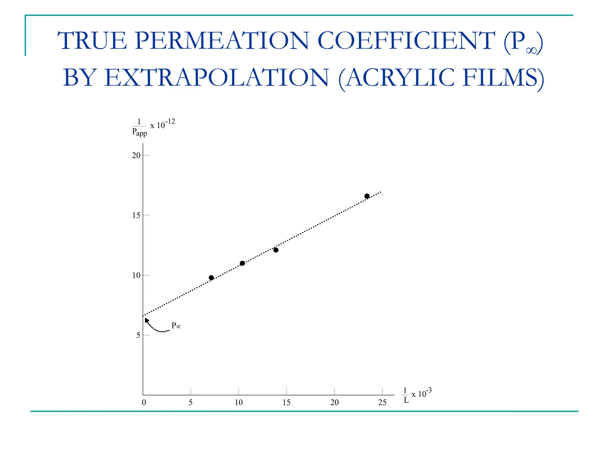
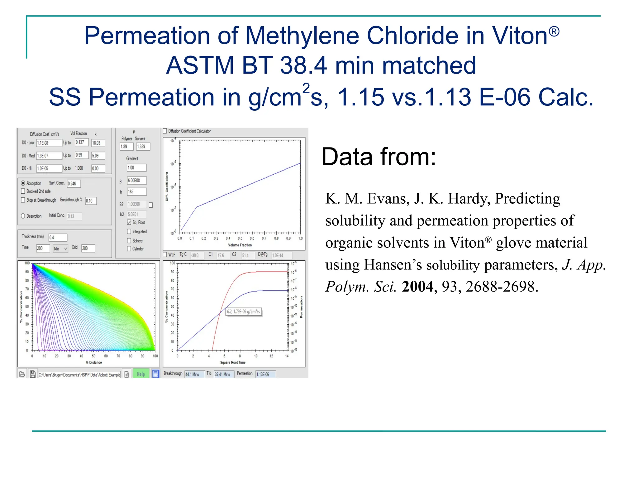
The document discusses the use of the diffusion equation to model various diffusion processes in polymers, focusing on solvent absorption, desorption, and permeation. It emphasizes the importance of concentration-dependent diffusion coefficients and surface effects in accurately predicting absorption behavior. The modeling results align with existing literature, demonstrating that the diffusion equation effectively captures complex diffusion phenomena in polymer systems.

1. Diffusion in Polymers 2020
The Diffusion Equation can model:
Absorption of solvent
Desorption of solvent
Permeation of solvent
Charles M. Hansen

2. OUTLINE
 Laws of Diffusion
 Find correct diffusion coefficients
 Concentration dependent coefficients
 Surface effects can be significant
 Combine these in diffusion equation to model
Film formation by solvent evaporation and
”Anomalies” of absorption (S-shaped, Case II).
Reliability of the modeling: The software in Hansen
Solubility Parameters in Practice (HSPiP) used here
gives the same results as are found in Crank (The
Mathematics of Diffusion) and analytical solutions.

3. FICK’S FIRST AND SECOND LAWS
Law 1: F = - D0(c/x)
For constant D0 in the x Direction, and
Law 2: c/t = /x (D0c/x)
This is also called the Diffusion Equation.
(Accumulation equals flux in minus flux out)
Calculations are referred to dry polymer.
Initial and 2 boundary conditions are required.
D0 can be replaced by exponential D(c).
Finding D(c) curve requires iteration for different c.

4. DIMENSIONLESS VARIABLES
Dimensionless time:
T = D0t/L2
(cm2
/s)(s/cm2
)
Dimensionless distance:
X = x/L
Dimensionless concentration:
C = (c – c0)/(c - c0)
L is the thickness of a free film

5. Absorption with a Constant Diffusion Coefficient
Straight line absorption - square root of time
(Diffusion coefficients upper right, Concentration
gradients lower left, absorption curve lower right)

6. Absorption with Exponential D(c)
Gives Advancing Front
Straight line absorption - square root of time

7. SURFACE CONDITION
Fs = h(Ceq
– Cs) = -DsCs/x
Flux through surface to(from) external phase, Fs,
equals flux through surface from(to) the bulk.
External Flux to/from surface, Fs, equals mass
transfer coefficient, h, (cm/s) times
concentration difference, g/cm
3
giving g/cm
2
s
Flux to/from bulk equals diffusion coefficient
(cm2
/s) times concentration gradient (g/cm3
cm)
h can be found from h = Fs /(Ceq
– Cs) @ t = 0

8. MEASURING DIFFUSION COEFFICIENTS
The Old Way: Correction Factors
The New Way: Curve Fitting
Half-time (t½) equation for measuring constant D0
D0 = 0.049 L2
/t½
For Concentration dependence multiply this by
Fa, for absorption, or Fd for desorption
For significant surface resistance multiply by FB
See also Nordtest POLY 188

9. CORRECTIONS FOR CONCENTRATION
DEPENDENCE ALONE
Note huge corrections for desorption
Desorption Absorption
Dmax/D0 (Fd)1/2 (Fd)1/4 (Fa)1/2
1 1.00 1.00 1.00
2 1.56 1.55 1.30
5 2.70 2.61 1.70
101
4.00 3.84 2.01
10
2
13.40 10.20 3.30
103
43.30 23.10 4.85
10
4
138.7 47.40 6.14
10
5
443.0 89.0 7.63
10
6
1,370.0 160.5 8.97
107
4,300.0 290.0 10.60
10
8
13,670.0 506.0 12.10
FB is a function of dimensionless surface parameter B = hL/D1
See Hansen, C.M., J.Appl Poly Sci, 26,3311-3315 (1981)

10. EXPONENTIAL DIFFUSION COEFFICIENTS FOR
CHLOROBENZENE IN POLY(VINYL ACETATE)
The system chlorobenzene in poly(vinyl acetate)
has been studied extensively with all relevant
data reported in my dissertation and subsequent
journal articles. The experiments were for:
Absorption from one equilibrium to another,
Desorption from different equilibrium values to
vacuum, and film drying (years).
Coherent understanding is found only by
accounting for concentration dependence and
significant surface effects when present.

11. CORRECTIONS: ABSORPTION 0.22 Vf to 0.27 Vf
(Fa) FOR D(c) AND FB FOR SURFACE EFFECTS

12. DESORPTION AND ABSORPTION GIVE SAME
D(c) WHEN CORRECTED (HANSEN 1967, 2007)
(Iteration Required)
14
12
10
8
6
-
LOG
diffusion
coefficient
at
20
°C,
cm²/sec
0.1 0.2 0.3 0.4 0.5 0.6
Desorption
(to vacuum)
Absorption
Isotope
F = 1.8
a
F = 40
d
F = 144
d
F = F x F
= 1.3 x 1.25
= 1.63
a B F = F x F
= 1.2 x 250
= 300
a B
Vf

13. D(c) FOR CHLOROBENZENE IN PVAc FOR
ALL CONCENTRATIONS (HANSEN, 1967)
-
LOG
D,
cm²/sec
0.2
Desorption
Absorption
Absorption
0.03 Vf
1 decade
~
0.2 Vf 1 decade
~
DAPP
DC
D1 (dry film)
Isotope
technique
Self-
diffusion
0 0.4 0.6 0.8 1.0
Vf
14
12
10
8
6
4

14. DRYING OF A LACQUER FILM
(Hansen, 1963, 1967, 1968)
10-7 10-6 10-5 10-4 10-3 10-2
10 -2
10 -1
10
101
B=106
B=107
CA CA
Exptl.
165 microns
Exptl.
22 microns
B=105
~ MO
CS = O
For B=107 CS = O
For B=106
CS = O
For B=105
Experimental
Calculated
One day L=30 microns
Effect of water - a steeper slope
DO t
(L) 2
T, Dimensionsless
Volume
Solvent
/
Volume
Polymer
V2 = 10 6
Vt = 10 10
CA = 0·2
B as indicated

15. RELATIVE SOLVENT RETENTION
DIFFUSION CONTROLED - SIZE/SHAPE
NOT HYDROGEN BONDING OR HSP
Cl
O
CH3
O
C
H3
OH
C
H3
C
H3
O
CH3
C
H3
CH3
CH3
O
CH3
CH3
CH3
O
C
H3
CH3
CH3
O
N
+
O O
CH3
C
H3
Cl
CH3
O
O
O
O
C
H3
O CH3
O
O
O
H
CH3
N
+
O O
CH3
O
O
H
CH3
C
H3
O
O
CH3
C
H3
N
+
O O
O
O
H CH3
C
H3
OH

16. WHOLE EQUALS SUM OF PARTS
E = COHESION ENERGY = ΔEvap
 E = ED + EP + EH
 D - Dispersion (Hydrocarbon)
 P - Polar (Dipolar)
 H - Hydrogen Bonds (Electron Interchange)
 V - Molar Volume
 E/V = ED/V + EP/V + EH/V

2
= 
2
D + 
2
P + 
2
H
HANSEN SOLUBILITY PARAMETERS (HSP)
 = Square Root of Cohesion Energy Density

17. POTENTIALLY SIGNIFICANT SURFACE
EFFECTS IN VAPOR ABSORPTION
 External phase diffusion from source to film
 Diffusion in stagnant boundary layer at film
 Heat removal on condensation
 Adsorption (How well do HSP match?)
 Orientation (Does n-hexane enter sideways?)
 Number of absorption sites, hole size and
shape, n-hexane sidewise?
 Transport into bulk (Diffusion coefficient,
molecular size and shape)

18. POTENTIALLY SIGNIFICANT SURFACE
EFFECTS IN (LIQUID) ABSORPTION
 Adsorption (How well do HSP match?)
 Polymer rotation to “match” HSP of external
phase: reason for success with a constant h?
 Orientation (Does n-hexane enter sideways?)
 Absorption site (hole size and shape)
 Number of absorption sites (h depends on
equilibrium uptake and similarity of HSP)
 Transport into bulk (Diffusion coefficient,
molecular size and shape)

19. ABSORPTION DELAY FOR LIQUID CONTACT
COC POLYMER TOPAS®
6013 TICONA
(NIELSEN, HANSEN 2005)
Absorption of selected solvents in a COC polymer
0
200
400
600
800
1000
1200
0 20 40 60 80 100 120 140 160
Sqrt time in min
Weight
change
in
mg/g
Hexane
THF
Diethylether
1,2-Dichloroethylene
0
100
200
300
0 5 10 15 20

20. Apparent h and Equilibrium Uptake for
COC Topas
®
6013 on Liquid Contact
Solvent Apparent h, cm/s Equilibrium uptake, vol.
fraction
Tetrahydrofuran 1.89(10)-4
0.676
Hexane 7.78(10)-6
0.351
Diethyl ether 1.21(10)-6
0.268
Propylamine 1.49(10)-7
0.181
Ethylene dichloride1.18(10)-7
0.176
Ethyl acetate 1.46(10)-8
0.076
n-Butyl acetate 8.30(10)-10
0.202
Phenyl acetate 0 0
Acetophenone 0 0
1,4-Dioxane 0 0
 Tetrahydrofuran: apparent h is too low since diffusion controls.
 n-Butyl acetate: apparent h is strongly lowered by size and shape.

21. Surface Mass Transfer COC (Topas
®
6013)
For Given Size Range, log(h) Depends on
Saturation Absorption, i.e. (ΔHSP)
0 0.1 0.2 0.3 0.4 0.5 0.6 0.7 0.8
-8
-7.5
-7
-6.5
-6
-5.5
-5
-4.5
-4
-3.5
-3
Correlation of log(h) with C
C (Saturated Vol Fraction)
log(h)

22. MAJOR REFERENCES EXPLAINING
“ANOMALIES” USING DIFFUSION EQUATION
Chapter 16 of Second Edition of Hansen Solubility
Parameters: A User’s Handbook, CRC Press, 2007.
Hansen CM. The significance of the surface condition in
solutions to the diffusion equation: explaining
"anomalous" sigmoidal, Case II, and Super Case II
absorption behavior. Eur Polym J 2010;46;651-662.
Abbott S, Hansen CM, Yamamoto H. Hansen Solubility
Parameters in Practice (HSPiP),
www.hansen-solubility.com. (The HSPiP package
includes validated software for absorption, desorption
and permeation.) One can curve fit data for films,
cylinders, and spheres.
Several downloads on www.hansen-solubility.com.

23. Thomas and Windle Case II Example
Methanol/PMMA with Iodine Tracer
Straight line absorption
with linear time cited as
excellent example of
Case II behavior.
This result is duplicated:
Diffusion equation with
iteration of both h and
exponential D(c). Stress
Explanation Not Correct

24. Methanol/PMMA Absorption at 30ºC
Diffusion Equation Simulation
“Breakthrough” 9.1 h, Gradients Flat at about 11 h

25. ”Experimental” Entry Coefficient, h
Methanol in PMMA
“Experimental” h is found from the straight line
(Case II) absorption data of Thomas and Windle
h = Fs /(Ceq
– Cs) @ t = 0 in cm/s
Ceq
= 0.24 %wgt; 0.373 gs/cm3
dry PMMA, Cs = 0
Ceq
= 0.265 vol fraction, 2x4 cm 2
=16cm2
surface
23 hours gives F = 2.09(10)-7
g/cm2
s
”Experimental” h = 5.6(10)-7
cm/s
”Topas” figure h = 7.0(10)-7
cm/s
Iterative modeling h = 11.0(10)-7
cm/s

26. Thomas and Windle Case II Example
Windle, “Case II Sorption” in Comyn, Polymer Permeability (1985)
Iodine tracer lags methanol
in PMMA at 30°C showing
apparent step-like gradient.
Methanol does not have this
“advancing sharp front”.
Iodine tracer is far too slow
as shown in the following.
Methanol gradients become
horizontal, not vertical.
Thickness: 930 microns

27. Effect of Molecular Properties on D0
Compare Methanol with Iodine

28. The Next Figure was
Reproduced from the Reference Below
Uptake of Methanol by Poly(methyl methacrylate):
An Old Problem Addressed by a Novel Raman
Technique
Jakob Nixdorf, Giuseppe Di Florio, Lars Bröckers, Carolin
Borbeck, Helen E. Hermes, Stefan U. Egelhaaf, and Peter
Gilch
Macromolecules 2019, 52, 13, 4997-5005
Heinrich-Heine University, Düsseldorf
FSRM (Femtosecond Stimulated Raman Microscopy)
Beam Focus at Middle of Disk Sample With
Sides Being Exposed

29. FSRM Raman Analysis of Concentration Profiles
Methanol in PMMA
”Breakthrough (BT)” at about 18+ hours

30. FSRM Raman Analysis of Concentration Profiles
Methanol in PMMA with Leakage at end
Surface Concentration about Doubled
Personal Communication from Peter Gilch

31. Prediction for FSRM Study, 1mm, Cylinder
D(c) and h from ”Thomas and Windle”
BT 21.1 h BT ca. 18+ h

32. For Calculated Horizontal Gradients at Left
to be found in Practice by (FSRM) at Right,
Ceq
MUST be about 0.265 volume fraction.
The FSRM Experiment on the Right was
NOT continued to equilibrium

33. Hopfenberg et.al. Super Case II
n-Hexane/Polystyrene (retained styrene)
C. H. M. Jacques, H. B. Hopfenberg,
V. T. Stannet, Vapor sorption and
liquid interactions with glassy
polyblends of Polystyrene and
Poly(2,6-Dimethyl-1,4-Phenylene
Oxide), Polym. Eng. Sci. 1973, 13(2)
(March), 81-87.
R. H. Holley, H. B. Hopfenberg,
V. Stannet, Anomalous transport
of hydrocarbons in Polystyrene.
Polym. Eng. Sci. 1970, 10(6)
(November), 376-382.

34. Hopfenberg and Coworkers Super Case II
“Closely” Modeled Absorption

35. PETROPOULOS et.al
Hansen cannot explain these data!
Stress mechanism given as cause of
“anomalous” behavior.
Petropoulos JH Sanopoulou M Papadokostaki KG.
Physically insightful modeling of non-Fickian
kinetic energy regimes encountered in
fundamental studies of isothermal sorption of
swelling agents in polymeric media.
Eur Polym J 2011;47:2053-2062.

36. Hansen cannot explain these data!
These slides do explain the data for liquid DCM
absorption into stretched, confined Cellulose Acetate
F = - D0(c/x) confirms leakage
D0 several times higher
than for liquid DCM
Concentration gradients
Stretched direction – step
Perpendicular due to leakage

37. CALCULATED ABSORPTION CURVE AND GRADIENTS
MATCH EXPERIMENTAL DATA FOR ABSORPTION
PERPENDICULAR TO STRETCH DIRECTION:
METHYLENE CHLORIDE IN CELLULOSE ACETATE

38. METHYLENE CHLORIDE IN STRETCH DIRECTION
CALCULATED ABSORPTION CURVE IS PERFECT, FRONT
NOT A SHARP STEP, BUT APPROACHES EXPERIMENTAL.
LACK OF ADHESION BETWEEN GLASS AND SAMPLE
IMPOSSIBLE D(c) TO APPROACH LEAKAGE RESULT!

39. Data: Hasimi et al. Eur.Polym.J. 2008;44:4098-4107
Diffusion Equation matches absorption of water into
bone dry PVAlc to 0.748 volume fraction
Stress Control is Unreasonable in liquid state!

40. Supercritical Carbon Dioxide 1µ PMMA
V. Carlà, et. al. Ind. Eng. Chem. Res. 2009, 48(8), 3844-3854
Total Surface Control
Bulk Explanation not Plausible

41. PERMEATION WITH SURFACE
AND/OR EXTERNAL RESISTANCES
F = p/(L/Papp) = p/(L/P + R1 + R2 + R3 …)
L/Papp = L/P + R1 + R2 + R3 ….
1/Papp = 1/P + (R1 + R2 + R3 ….)/L
Use Plot of 1/P Versus 1/L

42. TRUE PERMEATION COEFFICIENT (P∞)
BY EXTRAPOLATION (ACRYLIC FILMS)
20
15
10
5
0 5 10 15 20 25
P
Papp
1 x 10
-12
L
1 x 10
-3

43. Permeation of Methylene Chloride in Viton®
ASTM BT 38.4 min matched
SS Permeation in g/cm2
s, 1.15 vs.1.13 E-06 Calc.
Data from:
K. M. Evans, J. K. Hardy, Predicting
solubility and permeation properties of
organic solvents in Viton®
glove material
using Hansen’s solubility parameters, J. App.
Polym. Sci. 2004, 93, 2688-2698.

44. THE SCIENTIFIC CONCLUSION:
THE DIFFUSION EQUATION CAN MODEL
DIFFUSION IN POLYMERS
The diffusion equation has been shown to
fully model diffusion in many situations where
other explanations have been presented.
An advancing front concentration gradient in
absorption is caused by concentration
dependent diffusion coefficients.
A significant surface condition causes
absorption curves that are not linear with
square root of time.

45. THE PRACTICAL CONCLUSION
Mismatch Hansen solubility parameters to get
1. Lower equilibrium absorption, and therefore:
A. Lower concentration gradients
B. Lower diffusion coefficients
C. Lower surface entry coefficients
2. In practice, for drug and cosmetics packaging,
body suits, gloves, geomembranes, etc. Just -
Mismatch HSP for Better Barriers

46. SUMMARY
 Laws of Diffusion Valid for Diffusion in Polymers
 Exponential Diffusion Coefficients (D(c))
 Surface Condition (h) explains ”Anomalies”
 Combining D(c) and h - Complete Descriptions
 Estimate Behavior at Different Conditions
 Improved understanding and modeling of
absorption, desorption, and permeation
 Improve Barriers with (HSPp ≠ ≠ HSPs)

47. Thank you for your attention!
For further contact please visit:
www.hansen-solubility.com