This document is a thesis submitted by Debiprasad Ghosh for a Doctor of Philosophy degree in aerospace engineering at the Indian Institute of Science. The thesis examines using magnetostrictive sensors and actuators for structural health monitoring of composite structures. Composite materials are prone to damage, but damage can be difficult to detect. Traditional non-destructive testing methods have limitations. The thesis aims to develop a cost-effective, in-service system for monitoring composite structures using magnetostrictive materials. It will investigate extracting damage signatures from structural response histories using techniques like neural networks and dimension reduction.

1. Structural Health Monitoring of
Composite Structures using
Magnetostrictive Sensors and Actuators.
A Thesis
Submitted for the Degree of
Doctor of Philosophy
in the Faculty of Engineering
By
Debiprasad Ghosh
Department of Aerospace Engineering
Indian Institute of Science
Bangalore - 560 012
India
July 2006

2. Declaration
I declare that the thesis entitled Structural Health Monitoring of Composite
Structures Using Magnetostrictive Sensors and Actuators submitted by me for
the degree of Doctor of Philosophy in the Faculty of Engineering of Indian Institute of
Science, Bangalore did not form the subject matter of any other thesis submitted by me
for any outside degree, and the original work done by me and incorporated in this thesis
is entirely done at the Indian Institute of Science, Bangalore.
Bangalore
Debiprasad Ghosh
July 2006

3. Dedicated to
My Extended Family Members
and
My Teachers

4. Acknowledgements
I express my deep sense of gratitude and appreciation to Prof. S. Gopalakrishnan for
his excellent supervision, active participation, sustained interest and critical suggestions,
without which the thesis would not have come into its present shape. He gave me the
highest freedom that any advisor can allow for his student. He has always been very kind
and encouraging and his door was always open to me.
I am grateful to Prof. A. V. Krishna Murti and Dr. M. Kumar, for giving me the
opportunity to work with them and many of their valuable suggestions.
It is a great honour to have the opportunity to express my profound gratitude to Prof.
B. Dattaguru and Prof. T.S. Ramamurthy for the encouragement they offered to me
throughout my stay in the Department.
I thank Prof. B.N. Raghunandan, Chairman, Department of Aerospace Engineering, for
providing the department facilities and solving other official issues. I am also thankful
to all the scientific and administrative staff of the department throughout my study and
research work.
I thank Prof. N. Balakrishnan and Prof. S.M. Rao, former Chairman, SERC, for providing
all the computational facilities. I also thank all the present and former staff of SERC, for
their numerous help.
I am grateful to Prof. Manohar, Prof. Chandrakishan, Department of Civil Enginnering,
IISc, for their excellent teaching in the course of structural dynamics and finite element
analysis.
I thank Prof. Basudeb Datta, Department of Mathematics, IISc, for lending me the book
”Nonlinear electromechanical effects and applications”.
I thank my colleagues Dr. Joydeban, Dr. Krishna Lok Singh, Dr. K.V.N. Gopal, Dr.
Debiprosad Roy Mahapatra, Adris Bisi, Dr. Abir Chakraborty, Mira Mitra, Gudla, Power,
Guru, Promad, Niranjan, Murugan and Narashima for their numerous help throughout my
research work. I am thankful to my colleagues Sivaganyam for his valuable contributions
i

5. and ideas while working together on numerous research problems.
I am grateful to the families of Prof. Aloknath Chakraborty, Prof. Chandra and Prof.
Phoolan Prasad for their kind help at my off-campus staying.
I am grateful to Debiprasad Panda, Abhijit Chakraborty (C), Sauvikda, Abhijit Das
(barda), Subhas Pal of North Bengal University, Argha Nandi of Jadavpure Univer-
sity, Nandan Pakhira, Abhijit Chaudhuri (sonu), Abhijit Sarkar (galu), Alakesh (bhuto),
Amitabha, Bikash dey, Goutam (kanu), Nilanjan, Subhra, Suchi, Himadri Nandan Bar,
Joysurya (chhana), Sabita, Pinaki Biswas, Priyanko Ghosh, Rajesh Murarka, Saikat
(mama), Samit Baxi, Sarmistha, Sandipan (Mota), Saugata chakraborty, Bhat mama,
Santanu Biswas, Debashish Sarkar, Sayan Gupta, Sunetra Sarkar, Shyama, Siladitya Pal,
Sitikantha Roy, Sonjoy Das (soda), Dipankar, Santanu, Pallav, Luna, Kaushik (bachcha),
Suppriyo, Rajib (pagla), Sovan (bachcha), Surajit Midya, Subhankar, Subimal Ghosh,
Ayas, Rangeet, Ansuman, Sagarika, Tapas, Dipanyita, Pankaj, Tripti, Arnab and Ripa
who made my stay in the campus most memorable one.
Last but not the least I would like to express deep respect for my parents, parents-in-law,
my wife, my daughter and the other family members for their endearing support during
my tenure in IISc.

6. SYNOPSIS
Structural Health Monitoring of Composite
Structures Using Magnetostrictive Sensors and
Actuators.
Ph.D Thesis
Debiprasad Ghosh
S.R. No. 115199406
Department of Aerospace Engineering
Indian Institute of Science
Bangalore - 560012, INDIA
Fiber reinforced composite materials are widely used in aerospace, mechanical, civil and
other industries because of their high strength-to-weight and stiffness-to-weight ratios.
However, composite structures are highly prone to impact damage. Possible types of
defect or damage in composite include matrix cracking, fiber breakage, and delamination
between plies. In addition, delamination in a laminated composite is usually invisible. It
is very difficult to detect it while the component is in service and this will eventually lead
to catastrophic failure of the structure. Such damages may be caused by dropped tools
and ground handling equipments. Damage in a composite structure normally starts as a
tiny speckle and gradually grows with the increase in load to some degree. However, when
such damage reaches a threshold level, serious accident can occur. Hence, it is important
to have up-to-date information on the integrity of the structure to ensure the safety and
reliability of composite components, which require frequent inspections to identify and
quantify damage that might have occurred even during manufacturing, transportation or
storage.
How to identify a damage using the obtained information from a damaged compos-
ite structure is one of the most pivotal research objectives. Various forms of structural
damage cause variations in structural mechanical characteristics, and this property is ex-
tensively employed for damage detection. Existing traditional non-destructive inspection
techniques utilize a variety of methods such as acoustic emission, C-scan, thermography,
shearography and Moir interferometry etc. Each of these techniques is limited in accuracy
and applicability. Most of these methods require access to the structure. They also require

7. a significant amount of equipment and expertise to perform inspection. The inspections
are typically based on a schedule rather than based on the condition of the structure.
Furthermore, the cost associated with these traditional non-destructive techniques can
be rather prohibitive. Therefore, there is a need to develop a cost-effective, in-service,
diagnostic system for monitoring structural integrity in composite structures.
Structural health monitoring techniques based on dynamic response is being used
for several years. Changes in lower natural frequencies and mode shapes with their special
derivatives or stiffness/flexibility calculation from the measured displacement mode shapes
are the most common parameters used in identification of damage. But the sensitivity of
these parameters for incipient damage is not satisfactory. On the other hand, for in service
structural health monitoring, direct use of structural response histories are more suitable.
However, they are very few works reported in the literature on these aspects, especially
for composite structures, where higher order modes are the ones that get normally excited
due to the presence of flaws.
Due to the absence of suitable direct procedure, damage identification from response
histories needs inverse mapping; like artificial neural network. But, the main difficulty in
such mapping using whole response histories is its high dimensionality. Different general
purpose dimension reduction procedures; like principle component analysis or indepen-
dent component analysis are available in the literature. As these dimensionally reduced
spaces may loose the output uniqueness, which is an essential requirement for neural
network mapping, suitable algorithms for extraction of damage signature from these re-
sponse histories are not available. Alternatively, fusion of trained networks for different
partitioning of the damage space or different number of dimension reduction technique,
can overcome this issue efficiently. In addition, coordination of different networks trained
with different partitioning for training and testing samples, training algorithms, initial
conditions, learning and momentum rates, architectures and sequence of training etc., are
some of the factors that improves the mapping efficiency of the networks.
The applications of smart materials have drawn much attention in aerospace, civil,
mechanical and even bioengineering. The emerging field of smart composite structures
offers the promise of truly integrated health and usage monitoring, where a structure can
sense and adapt to their environment, loading conditions and operational requirements,
and materials can self-repair when damaged. The concept of structural health monitoring
using smart materials relies on a network of sensors and actuators integrated with the
structure. This area shows great promise as it will be possible to monitor the structural

8. condition of a structure, throughout its service lifetime. Integrating intelligence into
the structures using such networks is an interesting field of research in recent years.
Some materials that are being used for this purpose include piezoelectric, magnetostrictive
and fiber-optic sensors. Structural health monitoring using, piezoelectric or fiber-optic
sensors are available in the literature. However, very few works have been reported in the
literature on the use of magnetostrictive materials, especially for composite structures.
Non contact sensing and actuation with high coupling factor, along with other prop-
erties such as large bandwidth and less voltage requirement, make magnetostrictive ma-
terials increasingly popular as potential candidates for sensors and actuators in structural
health monitoring. Constitutive relationships of magnetostrictive material are represented
through two equations, one for actuation and other for sensing, both of which are coupled
through magneto-mechanical coefficient. In existing finite element formulation, both the
equations are decoupled assuming magnetic field as proportional to the applied current.
This assumption neglects the stiffness contribution coming from the coupling between
mechanical and magnetic domains, which can cause the response to deviate from the time
response. In addition, due to different fabrication and curing difficulties, the actual prop-
erties of this material such as magneto-mechanical coupling coefficient or elastic modulus,
may differ from results measured at laboratory conditions. Hence, identification of the
material properties of these embedded sensor and actuator are essential at their in-situ
condition.
Although, finite element method still remains most versatile, accurate and generally
applicable technique for numerical analysis, the method is computationally expensive for
wave propagation analysis of large structures. This is because for accurate prediction, the
finite element size should be of the order of the wavelength, which is very small due to high
frequency loading. Even in health monitoring studies, when the flaw sizes are very small
(of the order of few hundred microns), only higher order modes will get affected. This
essentially leads to wave propagation problem. The requirement of cost-effective compu-
tation of wave propagation brings us to the necessity of spectral finite element method,
which is suitable for the study of wave propagation problems. By virtue of its domain
transfer formulation, it bypasses the large system size of finite element method. Further,
inverse problem such as force identification problem can be performed most conveniently
and efficiently, compared to any other existing methods. In addition, spectral element
approach helps us to perform force identification directly from the response histories mea-
sured in the sensor. The spectral finite element is used widely for both elementary and

9. higher order one or two dimensional waveguides. Higher order waveguides, normally gives
a behavior, where a damping mode (evanescent) will start propagating beyond a certain
frequency called the cut-off frequency. Hence, when the loading frequencies are much be-
yond their corresponding cut-off frequencies, higher order modes start propagating along
the structure and should be considered in the analysis of wave propagations.
Based on these considerations, three main goals are identified to be pursued in this
thesis. The first is to develop the constitutive relationship for magnetostrictive sensor
and actuator suitable for structural analysis. The second is the development of differ-
ent numerical tools for the modelling the damages. The third is the application of these
developed elements towards solving inverse problems such as, material property identifica-
tion, impact force identification, detection and identification of delamination in composite
structure.
The thesis consists of four parts spread over six chapters. In the first part, linear,
nonlinear, coupled and uncoupled constitutive relationships of magnetostrictive materials
are studied and the elastic modulus and magnetostrictive constant are evaluated from
the experimental results reported in the literature. In uncoupled model, magnetic field
for actuator is considered as coil constant times coil current. The coupled model is
studied without assuming any explicit direct relationship with magnetic field. In linear
coupled model, the elastic modulus, the permeability and magnetostrictive coupling are
assumed as constant. In nonlinear-coupled model, the nonlinearity is decoupled and solved
separately for the magnetic domain and mechanical domain using two nonlinear curves,
namely the stress vs. strain curve and magnetic flux density vs. magnetic field curve.
This is done by two different methods. In the first, the magnetic flux density is computed
iteratively, while in the second, artificial neural network is used, where a trained network
gives the necessary strain and magnetic flux density for a given magnetic field and stress
level.
In the second part, different finite element formulations for composite structures
with embedded magnetostrictive patches, which can act both as sensors and actuators,
is studied. Both mechanical and magnetic degrees of freedoms are considered in the
formulation. One, two and three-dimensional finite element formulations for both coupled
and uncoupled analysis is developed. These developed elements are then used to identify
the errors in the overall response of the structure due to uncoupled assumption of the
magnetostrictive patches and shown that this error is comparable with the sensitivity
of the response due to different damage scenarios. These studies clearly bring out the

10. requirement of coupled analysis for structural health monitoring when magnetostrictive
sensor and actuator are used.
For the specific cases of beam elements, super convergent finite element formulation
for composite beam with embedded magnetostrictive patches is introduced for their spe-
cific advantages in having superior convergence and in addition, these elements are free
from shear locking. A refined 2-node beam element is derived based on classical and first
order shear deformation theory for axial-flexural-shear coupled deformation in asymmet-
rically stacked laminated composite beams with magnetostrictive patches. The element
has an exact shape function matrix, which is derived by exactly solving the static part
of the governing equations of motion, where a general ply stacking is considered. This
makes the element super convergent for static analysis. The formulated consistent mass
matrix, however, is approximate. Since the stiffness is exactly represented, the formulated
element predicts natural frequency to greater level of accuracy with smaller discretiza-
tion compared to other conventional finite elements. Finally, these elements are used for
material property identification in conjunction with artificial neural network.
In the third part, frequency domain analysis is performed using spectrally formu-
lated beam elements. The formulated elements consider deformation due to both shear
and lateral contraction, and numerical experiments are performed to highlight the higher
order effects, especially at high frequencies. Spectral element is developed for modelling
wave propagation in composite laminate in the presence of magnetostrictive patches. The
element, by virtue of its frequency domain formulation, can analyze very large domain
with nominal cost of computation and is suitable for studying wave propagation through
composite materials. Further more, identification of impact force is performed form the
magnetostrictive sensor response histories using these spectral elements.
In the last part, different numerical examples for structural health monitoring are
directed towards studying the responses due to the presence of the delamination in the
structure; and the identification of the delamination from these responses using artificial
neural network. Neural network is applied to get structural damage status from the
finite element response using its mapping feature, which requires output uniqueness. To
overcome the loss of output uniqueness due to the dimension reduction, damage space
is divided into different overlapped zones and then different networks are trained for
these zones. Committee machine is used to coordinate among these networks. Next, a
five-stage hierarchy of networks is used to consider partitioning of damage space, where
different dimension reduction algorithms and different partitioning between training and

11. testing samples are used for better mapping for the identification procedure. The results
of delamination detection for composite laminate show that the method developed in this
thesis can be applied to structural damage detection and health monitoring for various
industrial structures.
This thesis collectively addresses all aspects pertaining to the solution of inverse
problem and specially the health monitoring of composite structures using magnetostric-
tive sensor and actuator. In addition, the thesis discusses the necessity of higher order
theory in the high frequency analysis of wave propagation. The thesis ends with brief sum-
mary of the tasks accomplished, significant contribution made to the literature and the
future applications where the proposed methods addressed in this thesis can be applied.

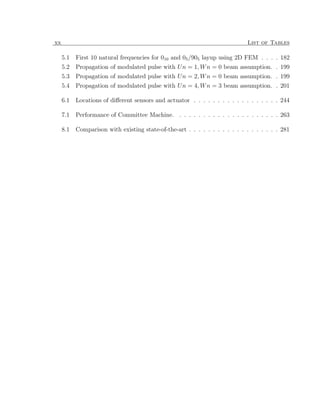
12. List of Publications
Journal papers
1. Ghosh D. P. and Gopalakrishnan S.; Role of Coupling in constitutive relationships
of magnetostrictive material. ”Computers, Materials & Continua, Vol.-1, No. 3, pp.
213-228”
2. Ghosh D. P. and Gopalakrishnan S.; Coupled analysis of composite laminate with
embedded magnetostrictive patches. Smart Materials and Structures 14 (2005)
1462-1473.
3. Ghosh D. P. and Gopalakrishnan S.; Super convergent finite element analysis of
composite beam with embedded magnetostrictive patches. Composite Structures
[in press].
4. Ghosh D. P. and Gopalakrishnan S.; Spectral finite element analysis of composite
beam with embedded magnetostrictive patches considering arbitrary order of shear
deformation and arbitrary order of poisson contraction. will be communicated
Conference papers
1. Ghosh D. P. and Gopalakrishnan S.; ”Structural health monitoring in a composite
beam using magnetostrictive material through a new FE formulation.” In Proceed-
ings of SPIE vol. 5062 Smart Materials, Structures and Systems, edited by San-
geneni Mohan, B. Dattaguru, S. Gopalakrishnan, (SPIE, Bellingham, WA, 2003)
and page number 704-711. ; Dec’12-14, 2002, Indian Institute of Science, Banga-
lore, India.
2. Ghosh D. P. and Gopalakrishnan S.; Time Domain Structural Health Monitoring
for Composite Laminate Using Magnetostrictive Material with ANN Modeling for
ix

13. Nonlinear Actuation Properties. Proceedings of INCCOM-2 & XII NASAS Sec-
ond ISAMPE national conference on composites and twelfth national seminar on
aerospace structures Sep’ 05-06, 2003, Bangalore, Karnataka, India
3. Ghosh D. P. and Gopalakrishnan S.; Identification of delamination size and location
of composite laminate from time domain data of magnetostrictive sensor and actu-
ator using artificial neural network. Proceeding of the SEC 2003, December 12-14,
structural engineering convention an international meet.
4. Ghosh D. P. and Gopalakrishnan S.; Time domain Structural Health Monitoring
with magnetostrictive patches using five-stage hierarchical neural network. Pro-
ceeding of the ICASI-2004, July 14-17,International Conference on Advances in
Structural Integrity.
5. Chakraborty A.; Ghosh D. P. and Gopalakrishnan S.; Damage Modelling And De-
tection Using Spectral Plate Element, International Congress on Computational
Mechanics and Simulation (ICCSM-2004). 9-12 December, 2004 at Indian Institute
of Technology Kanpur.

14. Contents
Acknowledgements i
SYNOPSIS iii
List of Publications ix
List of Tables xix
List of Figures xxi
1 Introduction 1
1.1 Motivation and Scope . . . . . . . . . . . . . . . . . . . . . . . . . . . . . . 1
1.2 Background: Structural Health Monitoring . . . . . . . . . . . . . . . . . . 2
1.2.1 Application Areas . . . . . . . . . . . . . . . . . . . . . . . . . . . . 4
1.2.1.1 Aerospace Application . . . . . . . . . . . . . . . . . . . . 4
1.2.1.2 Wind Turbine Blade Application . . . . . . . . . . . . . . 4
1.2.1.3 Bridge Structures . . . . . . . . . . . . . . . . . . . . . . . 4
1.2.1.4 Under Ground Structure . . . . . . . . . . . . . . . . . . . 5
1.2.1.5 Concrete Structure . . . . . . . . . . . . . . . . . . . . . . 5
1.2.1.6 Composite Structure . . . . . . . . . . . . . . . . . . . . . 6
1.2.2 Sensors and Actuators . . . . . . . . . . . . . . . . . . . . . . . . . 7
1.2.2.1 Piezoelectric Material . . . . . . . . . . . . . . . . . . . . 7
1.2.2.2 Optical Fiber . . . . . . . . . . . . . . . . . . . . . . . . . 7
1.2.2.3 Vibrometer . . . . . . . . . . . . . . . . . . . . . . . . . . 8
1.2.2.4 Magnetostrictive Material . . . . . . . . . . . . . . . . . . 8
1.2.2.5 Nano sensor . . . . . . . . . . . . . . . . . . . . . . . . . . 9
1.2.2.6 Comparisons of different sensors . . . . . . . . . . . . . . . 9
xi

15. xii Contents
1.2.3 Solution Domain . . . . . . . . . . . . . . . . . . . . . . . . . . . . 11
1.2.3.1 Static Domain . . . . . . . . . . . . . . . . . . . . . . . . 11
1.2.3.2 Modal domain . . . . . . . . . . . . . . . . . . . . . . . . 11
1.2.3.3 Frequency Domain . . . . . . . . . . . . . . . . . . . . . . 16
1.2.3.4 Time-Frequency Domain . . . . . . . . . . . . . . . . . . . 17
1.2.3.5 Impedance Domain . . . . . . . . . . . . . . . . . . . . . . 18
1.2.3.6 Time Domain . . . . . . . . . . . . . . . . . . . . . . . . . 19
1.2.4 Levels of SHM . . . . . . . . . . . . . . . . . . . . . . . . . . . . . . 19
1.2.4.1 Unsupervised SHM . . . . . . . . . . . . . . . . . . . . . . 19
1.2.4.2 Supervised SHM . . . . . . . . . . . . . . . . . . . . . . . 20
1.2.5 Damage Modelling in Composite Laminate . . . . . . . . . . . . . . 21
1.2.5.1 Matrix cracking . . . . . . . . . . . . . . . . . . . . . . . . 21
1.2.5.2 Techniques for Modelling of Delamination . . . . . . . . . 23
1.2.5.3 Multiple Delaminations . . . . . . . . . . . . . . . . . . . 25
1.2.6 Effective SHM Methodology . . . . . . . . . . . . . . . . . . . . . . 26
1.3 Background: Magnetostrictive Materials . . . . . . . . . . . . . . . . . . . 26
1.3.1 Initial History . . . . . . . . . . . . . . . . . . . . . . . . . . . . . . 27
1.3.2 Rare Earth Material Era . . . . . . . . . . . . . . . . . . . . . . . . 28
1.3.2.1 Giant Magnetostrictive Materials . . . . . . . . . . . . . . 28
1.3.3 Applications . . . . . . . . . . . . . . . . . . . . . . . . . . . . . . . 28
1.3.3.1 Thin Film and MEMS . . . . . . . . . . . . . . . . . . . . 29
1.3.3.2 Thick Film, Magnetostrictive Particle Composite . . . . . 30
1.3.4 Structural Applications . . . . . . . . . . . . . . . . . . . . . . . . . 30
1.3.4.1 Vibration and Noise Suppression . . . . . . . . . . . . . . 30
1.4 Artificial Neural Network . . . . . . . . . . . . . . . . . . . . . . . . . . . . 31
1.4.1 The Biological Inspiration . . . . . . . . . . . . . . . . . . . . . . . 32
1.4.2 The Basic Artificial Model . . . . . . . . . . . . . . . . . . . . . . . 32
1.4.3 Historical Background . . . . . . . . . . . . . . . . . . . . . . . . . 33
1.4.4 Neural Network Types . . . . . . . . . . . . . . . . . . . . . . . . . 34
1.4.4.1 Topology . . . . . . . . . . . . . . . . . . . . . . . . . . . 34
1.4.4.2 Connection Type . . . . . . . . . . . . . . . . . . . . . . . 34
1.4.4.3 Learning Methods . . . . . . . . . . . . . . . . . . . . . . 34
1.4.4.4 Applications . . . . . . . . . . . . . . . . . . . . . . . . . 35
1.4.5 Multi Layer Perceptrons (MLP) . . . . . . . . . . . . . . . . . . . . 35

16. Contents xiii
1.4.5.1 Transfer / Activation Function . . . . . . . . . . . . . . . 36
1.4.6 The Back-propagation Algorithm . . . . . . . . . . . . . . . . . . . 37
1.4.6.1 Training of BP ANN . . . . . . . . . . . . . . . . . . . . . 37
1.4.6.2 Sequential Mode . . . . . . . . . . . . . . . . . . . . . . . 39
1.4.6.3 Batch Mode . . . . . . . . . . . . . . . . . . . . . . . . . . 39
1.4.6.4 Validation of Trained Network . . . . . . . . . . . . . . . . 39
1.4.6.5 Execution of Trained Network . . . . . . . . . . . . . . . . 40
1.4.7 Applications for Neural Networks . . . . . . . . . . . . . . . . . . . 40
1.5 Objectives and Organization of the Thesis . . . . . . . . . . . . . . . . . . 41
2 Constitutive relationship of Magnetostrictive Materials 43
2.1 Introduction . . . . . . . . . . . . . . . . . . . . . . . . . . . . . . . . . . . 43
2.1.1 Existing Literature . . . . . . . . . . . . . . . . . . . . . . . . . . . 43
2.1.1.1 Coupling between Actuation and Sensing Equations . . . . 44
2.1.1.2 Nonlinearity of Magnetostrictive Materials . . . . . . . . . 45
2.1.1.3 Hysteresis of Magnetostrictive Materials . . . . . . . . . . 46
2.2 Uncoupled Constitutive Model . . . . . . . . . . . . . . . . . . . . . . . . . 48
2.2.1 Linear Uncoupled Model . . . . . . . . . . . . . . . . . . . . . . . . 50
2.2.1.1 Actuator Design - Some Issues . . . . . . . . . . . . . . . 52
2.2.1.2 Linearity . . . . . . . . . . . . . . . . . . . . . . . . . . . 52
2.2.1.3 Efficiency . . . . . . . . . . . . . . . . . . . . . . . . . . . 52
2.2.2 Polynomial Approach . . . . . . . . . . . . . . . . . . . . . . . . . . 54
2.2.3 ANN Model . . . . . . . . . . . . . . . . . . . . . . . . . . . . . . . 55
2.2.3.1 Network Architecture . . . . . . . . . . . . . . . . . . . . 55
2.2.3.2 Study on Number of Nodes in Hidden Layer . . . . . . . . 55
2.2.3.3 Study on Learning Rate . . . . . . . . . . . . . . . . . . . 58
2.2.3.4 Sequential Training Mode . . . . . . . . . . . . . . . . . . 58
2.2.3.5 Training by Batch Mode . . . . . . . . . . . . . . . . . . . 59
2.2.3.6 Momentum Effect . . . . . . . . . . . . . . . . . . . . . . 59
2.2.3.7 Selected Network . . . . . . . . . . . . . . . . . . . . . . . 59
2.2.4 Comparative Study with Polynomial Representation . . . . . . . . . 63
2.3 Coupled Constitutive Model . . . . . . . . . . . . . . . . . . . . . . . . . . 65
2.3.1 Linear Model . . . . . . . . . . . . . . . . . . . . . . . . . . . . . . 67
2.3.2 Nonlinear Coupled Model . . . . . . . . . . . . . . . . . . . . . . . 74

17. xiv Contents
2.3.3 ANN Model. . . . . . . . . . . . . . . . . . . . . . . . . . . . . . . . 82
2.3.4 Comparison between Different Coupled Models. . . . . . . . . . . . 83
2.4 Summary . . . . . . . . . . . . . . . . . . . . . . . . . . . . . . . . . . . . 85
3 FEM with Magnetostrictive Actuators and Sensors 87
3.1 Introduction . . . . . . . . . . . . . . . . . . . . . . . . . . . . . . . . . . . 87
3.1.1 Existing Literature . . . . . . . . . . . . . . . . . . . . . . . . . . . 87
3.2 3D Finite Element Formulation . . . . . . . . . . . . . . . . . . . . . . . . 88
3.2.1 Uncoupled Model . . . . . . . . . . . . . . . . . . . . . . . . . . . . 91
3.2.2 Coupled Model . . . . . . . . . . . . . . . . . . . . . . . . . . . . . 92
3.3 Computation of Sensor Open Circuit Voltage . . . . . . . . . . . . . . . . . 92
3.3.1 Uncoupled Model . . . . . . . . . . . . . . . . . . . . . . . . . . . . 93
3.3.2 Coupled Model . . . . . . . . . . . . . . . . . . . . . . . . . . . . . 93
3.4 Numerical Experiments . . . . . . . . . . . . . . . . . . . . . . . . . . . . . 94
3.4.1 Axial Deformation in a Magnetostrictive Rod . . . . . . . . . . . . 94
3.4.1.1 Uncoupled Analysis . . . . . . . . . . . . . . . . . . . . . 96
3.4.1.2 Coupled Analysis . . . . . . . . . . . . . . . . . . . . . . . 97
3.4.1.3 Degraded Composite Rod with Magnetostrictive Sensor/Actuator100
3.4.2 Finite Element Formulation for a Beam . . . . . . . . . . . . . . . . 100
3.4.2.1 Composite Beam with Magnetostrictive Bimorph . . . . . 104
3.4.2.2 Static Analysis . . . . . . . . . . . . . . . . . . . . . . . . 105
3.4.2.3 Frequency Response Analysis of a Healthy and Delami-
nated Beam . . . . . . . . . . . . . . . . . . . . . . . . . . 106
3.4.2.4 Time Domain Analysis . . . . . . . . . . . . . . . . . . . . 108
3.4.3 Finite Element Formulation of a Plate . . . . . . . . . . . . . . . . 111
3.4.3.1 Composite Plate with Magnetostrictive Sensor and Actuator116
3.4.4 Finite Element Formulation of 2D Plane Strain Elements . . . . . . 116
3.4.4.1 Composite Beam with Different Types of Failure . . . . . 118
3.5 Summary . . . . . . . . . . . . . . . . . . . . . . . . . . . . . . . . . . . . 121
4 Superconvergent Beam Element with Magnetostrictive Patches 122
4.1 Introduction . . . . . . . . . . . . . . . . . . . . . . . . . . . . . . . . . . . 122
4.1.1 Existing Literature . . . . . . . . . . . . . . . . . . . . . . . . . . . 123
4.2 Super-Convergent Finite Element Formulations. . . . . . . . . . . . . . . . 124
4.2.1 FE Formulation for Euler-Bernoulli Beam. . . . . . . . . . . . . . . 124

18. Contents xv
4.2.1.1 Uncoupled Formulation . . . . . . . . . . . . . . . . . . . 126
4.2.1.2 Coupled Formulation . . . . . . . . . . . . . . . . . . . . . 129
4.2.2 FE Formulation for First Order Shear Deformable (Timoshenko)
Beam . . . . . . . . . . . . . . . . . . . . . . . . . . . . . . . . . . 130
4.2.2.1 Uncoupled Formulation . . . . . . . . . . . . . . . . . . . 131
4.2.2.2 Coupled Formulation . . . . . . . . . . . . . . . . . . . . . 132
4.3 Numerical Experiments. . . . . . . . . . . . . . . . . . . . . . . . . . . . . 134
4.3.1 Static Analysis . . . . . . . . . . . . . . . . . . . . . . . . . . . . . 136
4.3.1.1 Euler-Bernoulli Beam . . . . . . . . . . . . . . . . . . . . 136
4.3.1.2 Timoshenko Beam . . . . . . . . . . . . . . . . . . . . . . 138
4.3.1.3 Single Element Performance for Static Analysis . . . . . . 139
4.3.2 Free Vibration Analysis. . . . . . . . . . . . . . . . . . . . . . . . . 141
4.3.2.1 Single Element Analysis. . . . . . . . . . . . . . . . . . . . 141
4.3.3 Super convergence Study. . . . . . . . . . . . . . . . . . . . . . . . 142
4.3.3.1 Free Vibration Analysis. . . . . . . . . . . . . . . . . . . . 142
4.3.3.2 Time History Analysis. . . . . . . . . . . . . . . . . . . . . 146
4.3.4 Material Property Identification . . . . . . . . . . . . . . . . . . . . 149
4.3.4.1 Elastic Modulus Identification . . . . . . . . . . . . . . . . 150
4.3.4.2 Magnetomechanical Coefficient Identification . . . . . . . 150
4.3.4.3 Material Properties Identification using ANN . . . . . . . 152
4.4 Summary . . . . . . . . . . . . . . . . . . . . . . . . . . . . . . . . . . . . 160
5 Spectral FE Analysis with Magnetostrictive Patches 162
5.1 Introduction . . . . . . . . . . . . . . . . . . . . . . . . . . . . . . . . . . . 162
5.1.1 Existing Literature . . . . . . . . . . . . . . . . . . . . . . . . . . . 164
5.2 FE Formulation of an nth Order Shear Deformable Beam with nth Order
Poisson’s Contraction . . . . . . . . . . . . . . . . . . . . . . . . . . . . . . 166
5.2.1 Conventional FE Matrices . . . . . . . . . . . . . . . . . . . . . . . 173
5.3 Spectral Finite Element Formulation of Beam . . . . . . . . . . . . . . . . 173
5.3.1 Closed Form Solution for Cut-off Frequencies . . . . . . . . . . . . . 175
5.3.2 Finite Length Element . . . . . . . . . . . . . . . . . . . . . . . . . 176
5.3.3 Semi-Infinite or Throw-Off Element . . . . . . . . . . . . . . . . . . 177
5.3.4 Effect of the Temperature Field . . . . . . . . . . . . . . . . . . . . 178
5.3.5 Effect of the Actuation Current . . . . . . . . . . . . . . . . . . . . 179

19. xvi Contents
5.3.6 Solution in the Frequency Domain . . . . . . . . . . . . . . . . . . . 179
5.3.6.1 Strain Computation . . . . . . . . . . . . . . . . . . . . . 179
5.3.6.2 Magnetic Field Calculation. . . . . . . . . . . . . . . . . . 180
5.3.6.3 Stress and Magnetic Flux Density Calculation. . . . . . . 181
5.3.6.4 Computation of Sensor Open Circuit Voltage. . . . . . . . 181
5.3.6.5 Time Derivatives of any Variable. . . . . . . . . . . . . . . 181
5.4 Numerical Results and Discussion . . . . . . . . . . . . . . . . . . . . . . . 182
5.4.1 Free Vibration and Wave Response Analysis . . . . . . . . . . . . . 182
5.4.1.1 Free Vibration Study . . . . . . . . . . . . . . . . . . . . . 184
5.4.1.2 Cut-Off Frequencies of Beam. . . . . . . . . . . . . . . . . 184
5.4.1.3 The Spectrum and Dispersion Relation . . . . . . . . . . . 188
5.4.1.4 Response to a Modulated Pulse . . . . . . . . . . . . . . . 196
5.4.1.5 Response to a Broad-band Pulse . . . . . . . . . . . . . . 203
5.4.2 Force Identification . . . . . . . . . . . . . . . . . . . . . . . . . . . 206
5.5 Summary . . . . . . . . . . . . . . . . . . . . . . . . . . . . . . . . . . . . 212
6 Forward SHM for Delamination 213
6.1 Introduction . . . . . . . . . . . . . . . . . . . . . . . . . . . . . . . . . . . 213
6.2 Delamination Modelling in Composite Laminate . . . . . . . . . . . . . . . 214
6.3 Numerical Example . . . . . . . . . . . . . . . . . . . . . . . . . . . . . . . 218
6.3.1 Tip Response Due to Tip Load . . . . . . . . . . . . . . . . . . . . 219
6.3.1.1 Varying Location . . . . . . . . . . . . . . . . . . . . . . . 219
6.3.1.2 Varying Size . . . . . . . . . . . . . . . . . . . . . . . . . 222
6.3.1.3 Symmetric Delaminations . . . . . . . . . . . . . . . . . . 222
6.3.1.4 Multiple Delaminations . . . . . . . . . . . . . . . . . . . 227
6.3.2 Sensor Response for a Tip Load . . . . . . . . . . . . . . . . . . . . 227
6.3.2.1 Varying Size and Layer . . . . . . . . . . . . . . . . . . . . 230
6.3.2.2 Varying Location . . . . . . . . . . . . . . . . . . . . . . . 230
6.3.2.3 Multiple Delaminations . . . . . . . . . . . . . . . . . . . 234
6.3.3 Tip Response for Actuation . . . . . . . . . . . . . . . . . . . . . . 234
6.3.3.1 Varying Location . . . . . . . . . . . . . . . . . . . . . . . 234
6.3.3.2 Varying Size . . . . . . . . . . . . . . . . . . . . . . . . . 238
6.3.4 Sensor Response for Actuation . . . . . . . . . . . . . . . . . . . . . 240
6.3.4.1 Varying Location . . . . . . . . . . . . . . . . . . . . . . . 240

20. Contents xvii
6.3.4.2 Varying Size and Layer . . . . . . . . . . . . . . . . . . . . 242
6.3.5 SHM of a Portal Frame . . . . . . . . . . . . . . . . . . . . . . . . . 244
6.3.5.1 Thin Portal Frame . . . . . . . . . . . . . . . . . . . . . . 245
6.3.5.2 Thick Portal Frame . . . . . . . . . . . . . . . . . . . . . 248
6.4 Summary . . . . . . . . . . . . . . . . . . . . . . . . . . . . . . . . . . . . 253
7 Structural Health Monitoring: Inverse Problem 255
7.1 Introduction . . . . . . . . . . . . . . . . . . . . . . . . . . . . . . . . . . . 255
7.2 SHM using Single ANN . . . . . . . . . . . . . . . . . . . . . . . . . . . . . 257
7.2.1 Difficulties in Single ANN . . . . . . . . . . . . . . . . . . . . . . . 259
7.3 Committee Machine . . . . . . . . . . . . . . . . . . . . . . . . . . . . . . 262
7.3.1 Numerical Experiment using Committee Machine . . . . . . . . . . 263
7.3.2 Information Loss due to Dimension Reduction . . . . . . . . . . . . 267
7.4 Hierarchical Neural Network (HNN) . . . . . . . . . . . . . . . . . . . . . . 268
7.4.1 Five Stage HNN . . . . . . . . . . . . . . . . . . . . . . . . . . . . . 268
7.4.1.1 Neural Networks . . . . . . . . . . . . . . . . . . . . . . . 268
7.4.1.2 Ensemble Network . . . . . . . . . . . . . . . . . . . . . . 268
7.4.1.3 Validation Network . . . . . . . . . . . . . . . . . . . . . . 269
7.4.1.4 Expert in HNN . . . . . . . . . . . . . . . . . . . . . . . . 270
7.4.1.5 Committee Machine in HNN . . . . . . . . . . . . . . . . 271
7.4.2 Training Phase of HNN . . . . . . . . . . . . . . . . . . . . . . . . . 271
7.4.2.1 Training of ANN . . . . . . . . . . . . . . . . . . . . . . . 271
7.4.2.2 Training of Ensembler Network . . . . . . . . . . . . . . . 272
7.4.3 Testing Phase of HNN . . . . . . . . . . . . . . . . . . . . . . . . . 273
7.4.3.1 Testing of ANN . . . . . . . . . . . . . . . . . . . . . . . . 273
7.4.3.2 Testing of Ensembler Network . . . . . . . . . . . . . . . . 273
7.4.3.3 Testing of Validation Network . . . . . . . . . . . . . . . . 273
7.4.4 Execution Phase of HNN . . . . . . . . . . . . . . . . . . . . . . . . 274
7.4.4.1 Execution of ANN . . . . . . . . . . . . . . . . . . . . . . 274
7.4.4.2 Execution of Ensembler Network . . . . . . . . . . . . . . 274
7.4.4.3 Execution of Validation Network . . . . . . . . . . . . . . 274
7.4.4.4 Execution of Expert Network . . . . . . . . . . . . . . . . 275
7.4.4.5 Active Expert Network . . . . . . . . . . . . . . . . . . . . 275
7.4.5 Numerical Study of Five Stage Hierarchical ANN . . . . . . . . . . 276

21. xviii Contents
7.5 Summary . . . . . . . . . . . . . . . . . . . . . . . . . . . . . . . . . . . . 277
8 Summary and Future Scope of Research 278
8.1 Contribution of the Thesis . . . . . . . . . . . . . . . . . . . . . . . . . . . 280
8.1.1 Limitation of the Approach . . . . . . . . . . . . . . . . . . . . . . 282
8.2 Future Scope of Research . . . . . . . . . . . . . . . . . . . . . . . . . . . . 282
Appendices 284
A Euler-Bernoulli Beam 285
B Timoshenko Beam 288
C Higher Order Theories 292
References 301

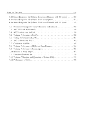
22. List of Tables
1.1 Comparison of different smart materials for SHM application. . . . . . . . 10
2.1 Constants α0 through α4 for different prestress levels [192]. . . . . . . . . . 54
2.2 Connection between input layer and hidden layer. . . . . . . . . . . . . . . 63
2.3 Connection between hidden layer and output layer. . . . . . . . . . . . . . 63
2.4 Coefficients for sixth order polynomial. . . . . . . . . . . . . . . . . . . . . 78
2.5 Connection between input layer and hidden layer. . . . . . . . . . . . . . . 83
2.6 Connection between hidden layer and output layer. . . . . . . . . . . . . . 85
3.1 Vertical Displacement of Cantilever Tip . . . . . . . . . . . . . . . . . . . . 105
4.1 Tip Deflection (mm) for Static Tip Load of 1 kN . . . . . . . . . . . . . . 140
4.2 Tip Deflection (mm) for Static Tip Load of 1 kN . . . . . . . . . . . . . . 140
4.3 Tip Deflection (mm) for Actuation Current . . . . . . . . . . . . . . . . . . 141
4.4 First Three Natural Frequencies (Hz) . . . . . . . . . . . . . . . . . . . . . 142
4.5 First Three Natural Frequencies (Hz) . . . . . . . . . . . . . . . . . . . . 142
4.6 First peak amplitude of training samples (mili-volt) . . . . . . . . . . . . . 154
4.7 Middle peak amplitude of training samples (mili-volt) . . . . . . . . . . . . 154
4.8 Middle peak location of training samples (micro-second) . . . . . . . . . . 154
4.9 Last peak amplitude of training samples (mili-volt) . . . . . . . . . . . . . 155
4.10 Last peak location of training samples (micro-second) . . . . . . . . . . . . 155
4.11 First peak amplitude of validation samples (mili-volt) . . . . . . . . . . . . 157
4.12 Middle peak amplitude of validation samples (mili-volt) . . . . . . . . . . . 157
4.13 Middle peak location of validation samples (micro-second) . . . . . . . . . 157
4.14 Last peak amplitude of validation samples (mili-volt) . . . . . . . . . . . . 160
4.15 Last peak location of validation samples (micro-second) . . . . . . . . . . . 160
xix

23. xx List of Tables
5.1 First 10 natural frequencies for 010 and 05 /905 layup using 2D FEM . . . . 182
5.2 Propagation of modulated pulse with U n = 1, W n = 0 beam assumption. . 199
5.3 Propagation of modulated pulse with U n = 2, W n = 0 beam assumption. . 199
5.4 Propagation of modulated pulse with U n = 4, W n = 3 beam assumption. . 201
6.1 Locations of different sensors and actuator . . . . . . . . . . . . . . . . . . 244
7.1 Performance of Committee Machine. . . . . . . . . . . . . . . . . . . . . . 263
8.1 Comparison with existing state-of-the-art . . . . . . . . . . . . . . . . . . . 281

24. List of Figures
1.1 Magnetostriction due to switching of magnetic domains. . . . . . . . . . . 27
1.2 Artificial Neural Network of 7-14-7 Architecture. . . . . . . . . . . . . . . . 38
2.1 Magnetostriction vs. magnetic field supplied by Etrema . . . . . . . . . . . 49
2.2 Magneto-mechanical coupling vs. magnetic field supplied by Etrema . . . . 50
2.3 Stress vs. strain relationship for different magnetic field level [Etrema] . . . 51
2.4 Elasticity vs. strain relationship for different magnetic field level [Etrema] . 51
2.5 Tangential coupling with bias field for different stress level. . . . . . . . . . 53
2.6 Coupling coefficient with bias field for different stress level. . . . . . . . . . 53
2.7 Study on the effect of number of node in hidden layer. . . . . . . . . . . . 56
2.8 Study on the effect of number of node in hidden layer. . . . . . . . . . . . 56
2.9 Test data from network and sample data set. . . . . . . . . . . . . . . . . . 57
2.10 Test data from network and sample data set. . . . . . . . . . . . . . . . . . 57
2.11 Effect of learning rate on training performance . . . . . . . . . . . . . . . . 60
2.12 Effect of learning rate on validation performance . . . . . . . . . . . . . . . 60
2.13 Effect of learning rate on batch mode training performance. . . . . . . . . 61
2.14 Effect of learning rate on validation performance for batch mode learning. . 61
2.15 Effect of momentum on training performance. . . . . . . . . . . . . . . . . 62
2.16 Effect of momentum on training performance. . . . . . . . . . . . . . . . . 62
2.17 Magnetostriction for different stress level. . . . . . . . . . . . . . . . . . . . 64
2.18 Coupling coefficient for different stress level. . . . . . . . . . . . . . . . . . 64
2.19 Magnetostriction for different stress level. . . . . . . . . . . . . . . . . . . . 66
2.20 Ratio of two permeabilities (r) with different values of permeability vs.
modulus of elasticity (a) and modified elasticity (b), considering d=15X10−9
m/Amp . . . . . . . . . . . . . . . . . . . . . . . . . . . . . . . . . . . . . . 71
xxi

25. xxii List of Figures
2.21 Ratio of two permeabilities (r) with different values of coupling coefficient
vs. constant strain permeability (a) and constant stress permeability (b),
considering Q=15GPa. . . . . . . . . . . . . . . . . . . . . . . . . . . . . . 72
2.22 Ratio of two permeabilities (r) with different values of coupling coefficient
vs. modulus of elasticity (a) and modified elasticity (b), considering µ =
7X10−6 henry/m. . . . . . . . . . . . . . . . . . . . . . . . . . . . . . . . . 73
2.23 Nonlinear curves (a) Strain vs. Stress curve (b) Magnetic field vs. Magnetic
flux density curve. . . . . . . . . . . . . . . . . . . . . . . . . . . . . . . . 79
2.24 Nonlinear curves in different stress level (a) Magnetic field vs. Strain (b)
Magnetic field vs. Magnetostriction. . . . . . . . . . . . . . . . . . . . . . . 80
2.25 Nonlinear curves for different field level (a) Stress vs. Strain (b) Modulus
vs. Strain. . . . . . . . . . . . . . . . . . . . . . . . . . . . . . . . . . . . . 81
2.26 Artificial neural network architecture . . . . . . . . . . . . . . . . . . . . . 83
2.27 Nonlinear curves for different stress level (a) Strain vs. Magnetic field (b)
Magnetic flux density vs. Magnetic field. . . . . . . . . . . . . . . . . . . . 84
3.1 Various elements with node and degrees of freedom. . . . . . . . . . . . . . 95
3.2 Composite Rod With Magnetostrictive Sensor and Actuator . . . . . . . . 99
3.3 Open Circuit Voltages at Magnetostrictive Sensor . . . . . . . . . . . . . . 99
3.4 Laminated Beam With Magnetostrictive Patches. . . . . . . . . . . . . . . 104
3.5 Frequency Response Function . . . . . . . . . . . . . . . . . . . . . . . . . 107
3.6 Actuation History with Frequency content . . . . . . . . . . . . . . . . . . 109
3.7 Cantilever Tip Velocity for 00 ply angle . . . . . . . . . . . . . . . . . . . . 110
3.8 Cantilever Tip Velocity for 900 ply angle. . . . . . . . . . . . . . . . . . . . 112
3.9 Sensor Open Circuit Voltage for 00 ply angle . . . . . . . . . . . . . . . . . 113
3.10 Sensor Open Circuit Voltage for 900 ply angle . . . . . . . . . . . . . . . . 114
3.11 Multiple delaminated plate with magnetostrictive sensor and actuator . . . 117
3.12 Sensor open circuit voltage for plate with multiple delaminations . . . . . . 117
3.13 Laminated composite beam with sensor, actuator and crack . . . . . . . . 119
3.14 Sensor open circuit voltages for matrix crack in laminated composite beam 119
3.15 Sensor Open Circuit Voltages for Fiber Breakage . . . . . . . . . . . . . . . 120
3.16 Sensor Open Circuit Voltages for Internal Crack . . . . . . . . . . . . . . . 120
4.1 10 layer composite cantilever beam with different layup sequence . . . . . . 137
4.2 Natural Frequency for Cantilever Beam with [010 ] Layup sequence . . . . . 143

26. List of Figures xxiii
4.3 Natural Frequency for Cantilever Beam with [05 /905 ] Layup sequence . . . 143
4.4 Natural Frequency for Beam with Coupled, [m/08 /m] Layup sequence . . . 144
4.5 Natural Frequency for Beam with Uncoupled, [m/08 /m] Layup sequence . 144
4.6 Natural Frequency for Beam with Coupled, [m/04 /904 /m] Layup sequence 145
4.7 Natural Frequency for Beam with Uncoupled, [m/04 /904 /m] Layup sequence145
4.8 50 kHz Broadband Force History with Frequency Content (inset) . . . . . . 147
4.9 Effect of Beam Assumption on Tip Response [010 ] . . . . . . . . . . . . . . 147
4.10 Superconvergent Study of ScFSDT elements . . . . . . . . . . . . . . . . . 148
4.11 Open circuit voltage for Coupled, [m/08 /s] Layup sequence . . . . . . . . . 149
4.12 Sensor voltage for coupled, [m/04 /904 /s] with varying elasticity . . . . . . 151
4.13 Sensor voltage for Coupled, [m/04 /904 /s] with varying coupling coefficient 151
4.14 Open circuit voltage for Coupled, [m/04 /904 /s] layup sequence . . . . . . . 152
4.15 Training Histories of different ANN architectures . . . . . . . . . . . . . . 156
4.16 ANN with Different architectures . . . . . . . . . . . . . . . . . . . . . . . 158
4.17 Training Performance of 5-4-2 ANN architectures . . . . . . . . . . . . . . 159
4.18 Validation Performance of 5-4-2 ANN architectures . . . . . . . . . . . . . 159
5.1 Error in Natural Frequency for Different Beam Assumptions . . . . . . . . 183
5.2 Cut-Off Frequencies for [010 ] Layup with different beam assumptions. . . . 185
5.3 Cut-Off Frequencies for [m/04 /904 /m] layup with different beam assump-
tions. . . . . . . . . . . . . . . . . . . . . . . . . . . . . . . . . . . . . . . . 186
5.4 Spectrum Relationships and Group Speeds for [010 ]. . . . . . . . . . . . . . 189
5.5 Spectrum Relationships and Group Speeds for [010 ]. . . . . . . . . . . . . . 190
5.6 Spectrum Relationships and Group Speeds for [m/04 /904 /m]. . . . . . . . 192
5.7 Group Speed for [m/04 /904 /m] Layup sequence. . . . . . . . . . . . . . . . 194
5.8 Group Speed for [m/04 /904 /m] Layup sequence. . . . . . . . . . . . . . . . 195
5.9 Modulated pulse of 200 kHz frequency . . . . . . . . . . . . . . . . . . . . 197
5.10 Group Speed and Modulated Pulse Response for [m/04 /904 /m] Layup with
U n = 1, W n = 0. . . . . . . . . . . . . . . . . . . . . . . . . . . . . . . . . 198
5.11 Group Speed and Modulated Pulse Response for [m/04 /904 /m] Layup with
U n = 2, W n = 0. . . . . . . . . . . . . . . . . . . . . . . . . . . . . . . . . 200
5.12 Group Speed and Modulated Pulse Response for [m/04 /904 /m] Layup with
U n = 4, W n = 3. . . . . . . . . . . . . . . . . . . . . . . . . . . . . . . . . 202
5.13 Broadband response of 010 layup sequence. . . . . . . . . . . . . . . . . . . 204
5.14 Broadband response of [m/04 /904 /s] layup sequence (s for sensor layer). . 205

27. xxiv List of Figures
5.15 25 kHz Broadband Force Reconstruction for [m/04 /904 /m] layup. . . . . . 211
6.1 Modelling of Delamination in Finite Element Formulation. . . . . . . . . . 215
6.2 Comparison between Beam and 2D Modelling of Delamination . . . . . . . 217
6.3 Composite Beam with Sensor and Actuator . . . . . . . . . . . . . . . . . 218
6.4 100mm Delamination at Mid Layer and Different Distance from Support. . 220
6.5 20mm Delamination at Mid Layer and Different Distance from Support. . . 221
6.6 Delamination at Mid span of Mid Layer with Different sizes. . . . . . . . . 223
6.7 Delamination at Mid span of Top Layer with Different sizes. . . . . . . . . 224
6.8 Symmetric Delaminations at Top and Bottom Layers. . . . . . . . . . . . . 225
6.9 Symmetric Delaminations at ± 0.3mm Layers. . . . . . . . . . . . . . . . . 226
6.10 Multiple Delaminations Increasing towards the Depth. . . . . . . . . . . . 228
6.11 20, 50 and 100mm Delamination at mid and top Layer near Support. . . . 229
6.12 100mm Top Layer Delamination for Different Distance from Support. . . . 231
6.13 100mm Mid Layer Delamination for Different Distance from Support. . . . 232
6.14 100mm Bottom Layer Delamination for Different Distance from Support. . 233
6.15 20mm Top Layer Delamination for Different Distance from Support. . . . . 235
6.16 Multiple Delaminations Increasing towards the Depth . . . . . . . . . . . . 236
6.17 100mm Delamination at Top layer for 50 Hz and 5kHz Actuation. . . . . . 237
6.18 100mm Delamination at Mid layer for 50 Hz and 5kHz Actuation. . . . . . 237
6.19 100mm Delamination at Bottom layer for 50 Hz and 5kHz Actuation. . . . 237
6.20 Delamination at Top layer near support for 50 Hz and 5kHz Actuation. . . 239
6.21 Delamination at Mid layer near support for 50 Hz and 5kHz Actuation. . . 239
6.22 Delamination at Bottom layer near support for 50 Hz and 5kHz Actuation. 239
6.23 100mm Delamination at Top layer for 50 Hz and 5kHz Actuation. . . . . . 241
6.24 100mm Delamination at Mid layer for 50 Hz and 5kHz Actuation. . . . . . 241
6.25 100mm Delamination at Bottom layer from support to 200mm for 50 Hz
and 5kHz Actuation. . . . . . . . . . . . . . . . . . . . . . . . . . . . . . . 241
6.26 Delamination at Top layer near support for 50 Hz and 5kHz Actuation. . . 243
6.27 Delamination at Mid layer near support for 50 Hz and 5kHz Actuation. . . 243
6.28 Delamination at Bottom layer near support for 50 Hz and 5kHz Actuation. 243
6.29 Delaminated Composite Portal Frame with Sensors and Actuator . . . . . 244
6.30 Sensor Responses for Different Beam Assumptions. . . . . . . . . . . . . . 246
6.31 Sensor Responses for Different Locations of Sensors with EB Assumption. . 247
6.32 Sensor Responses for Different Locations of Sensors with FSDT Assumption.249

28. List of Figures xxv
6.33 Sensor Responses for Different Locations of Sensors with 2D Model. . . . . 250
6.34 Sensor Responses for Different Beam Assumptions. . . . . . . . . . . . . . 251
6.35 Sensor Responses for Different Locations of Sensors with 2D Model. . . . . 252
7.1 Delaminated composite beam with sensor and actuator. . . . . . . . . . . . 258
7.2 ANN of 10-5-1 Architecture. . . . . . . . . . . . . . . . . . . . . . . . . . . 259
7.3 ANN Architecture 10-5-2-1. . . . . . . . . . . . . . . . . . . . . . . . . . . 259
7.4 Training Performance of ANNs. . . . . . . . . . . . . . . . . . . . . . . . . 260
7.5 Testing Performance of ANNs. . . . . . . . . . . . . . . . . . . . . . . . . . 261
7.6 ANN Architecture 10-5-2. . . . . . . . . . . . . . . . . . . . . . . . . . . . 262
7.7 Committee Machine. . . . . . . . . . . . . . . . . . . . . . . . . . . . . . . 262
7.8 Training Performance of Different Span Experts. . . . . . . . . . . . . . . . 264
7.9 Training Performance of span experts . . . . . . . . . . . . . . . . . . . . . 265
7.10 Removal of Noisy Expert. . . . . . . . . . . . . . . . . . . . . . . . . . . . 267
7.11 Partition of Sample Set. . . . . . . . . . . . . . . . . . . . . . . . . . . . . 270
7.12 Training, Validation and Execution of 5 stage HNN. . . . . . . . . . . . . . 272
7.13 Performance of HNN. . . . . . . . . . . . . . . . . . . . . . . . . . . . . . . 276

29. Chapter 1
Introduction
1.1 Motivation and Scope
Composites have revolutionized structural construction. They are extensively used in
aerospace, civil, mechanical and other industries. Present day aerospace vehicles have
composites upto 60 % or more of the total material used. More recently, materials, which
can give rise to mechanical response when subjected to non-mechanical loads such as
PZTs, magnetostrictive, SMAs, have become available. Such materials may broadly refer
to as functional materials. With the availability of functional materials and the feasibility
of embedding those into or bonding those to composite structures, smart structural con-
cepts are emerging to be attractive for potential high performance structural applications
[236]. A smart structure may be generally defined as one which has the ability to deter-
mine its current state, decides in a rational manner on a set of actions that would change
its state to a more desirable state and carries out these actions in a controlled manner in a
short period of time. With such features incorporated in a structure by embedding func-
tional materials, it is feasible to achieve technological advances such as vibration and noise
reduction, high pointing accuracy of antennae, damage detection, damage mitigation etc.
[128, 45].
Various damages like crack or delamination in composite structures are unavoidable
during service time due to the impact or continual load, chemical corrosion and aging,
change of ambient conditions, etc. These damages will cause a change in the strain/stress
state of the structure and hence its vibration characteristics. By continuously monitoring
one or more of these response quantities, it is possible to assess the condition of the
structure for its structural integrity. Such a monitoring of the structure is called structural
health monitoring. Health monitoring application has received great deal of attention all
over the world, due to its significant impact on safety and longevity of the structure.
1

30. 2 Chapter 1. Introduction
To implement health monitoring concept, it is necessary to have a number of sensors
to measure response parameters. These response will then be post-processed to asses
the condition of structure. Such a system was built by Lin and Chang [232], when
they developed a built-in monitoring system for composite structures using a network
of actuators or sensors. The engineering community has great interest in the development
of new real-time, in-service health monitoring techniques to reduce cost and improve
safety. With the current NDE techniques, the complex mechanical systems need to be
taken out of service for an extended period of time for the inspection. The inspection
becomes even more lengthy and expensive for inaccessible locations. Also, on the same
preventive basis, structures are often withdrawn from service early, even if the structure is
still capable of performing its task. It is estimated that nearly 27 percent of an aircraft’s
life cycle cost is spent on inspections and repairs (Kessler et al. [178]). With an on-line,
self actuated system, such costs can be dramatically reduced. Furthermore, the impact
of such an in-situ SHM system is that it not only increases safety and performance, but
also enables converting schedule based into condition based maintenance, thus reducing
both down time and costs (Bray and Roderick [46]).
The overall objective of this thesis is how magnetostrictive sensor responses can be
used to identify the health condition of the composite structures. So, the central question
is how responses can be obtained for both healthy or damaged structures, which is forward
analysis; and how these obtained responses can be mapped with the damage state of the
structure, which is inverse problem. Hence, different 1D, 2D and 3D finite element is
formulated to get magnetostrictive sensor responses for healthy and damaged structures
with mapping of different artificial neural networks for identification of damages. Sensing
and actuation properties are characterized using available experimental results. Optimal
location of sensors are studied in structural health monitoring framework. In addition,
in-situ sensor properties and applied forces on structures are identified from truncated
sensor responses.
1.2 Background: Structural Health Monitoring
The safety and performance of all commercial, civil, and military structural systems dete-
riorate with time. Further more, it is very important to confirm the structural condition
immediately by nondestructive inspection or other method when the structure receives
the foreign object collision. Structural damage detection at the earliest possible stage is

31. 1.2. Background: Structural Health Monitoring 3
very important in the aerospace industry to prevent major failures and for this reason it
has attracted a lot of interest. However, it is not practical to assume experts are always
available to explain the measured data. With the advances in sensor systems, data ac-
quisition, data communication and computational methodologies, instrumentation-based
monitoring has been a widely accepted technology to monitor and diagnose structural
health and conditions for civil, aerospace and mechanical structural systems. The process
of implementing a damage detection strategy for aerospace, civil, and mechanical engi-
neering infrastructure is referred to as Structural Health Monitoring (SHM). Followings
are some of the facts attributed to SHM:
• SHM is the whole process of the design, development and implementation of tech-
niques for the detection, localization and estimation of damages, for monitoring the
integrity of structures and machines.
• Because of current manual inspection and maintenance scheduling procedures are
time consuming, costly, insensitive to small variations in structural health, and prone
to error in severe and mild operating environments, there is an urgent economic and
technological need to deploy automated structural diagnostic instrumentation for
seamless evaluation of structural integrity and reliability.
• SHM offers the promise of a paradigm shift from schedule-driven maintenance to
condition-based maintenance of structures.
• The concept of SHM is a technology that automatically monitors structural condi-
tions from sensor information in real-time, by equipping sensor network and diag-
nosis algorithms into structures.
• The key requirements of a health monitoring system are that it should be able to
detect damaging events, characterize the nature, extent and seriousness of the dam-
age, and respond intelligently on whatever timescale is required, either to mitigate
the effects of the damage or to effect its repair.
Doebling et al. [100, 101] provide one of the most comprehensive reviews of the
technical literature concerning the detection, location, and characterization of structural
damage through techniques that examine changes in measured structural-vibration re-
sponse.

32. 4 Chapter 1. Introduction
1.2.1 Application Areas
1.2.1.1 Aerospace Application
SHM for Aerospace structures are studied by many researchers. Qing et al. [317] had
developed a hybrid piezoelectric/fiber optic diagnostic system for quick non-destructive
evaluation and long term health monitoring of aerospace vehicles and structures. The
SHM system for the Eurofighter Typhoon had been reported by Hunt and Hebden [164].
Fujimoto and Sekine [125] presented a method for identification of the locations and
shapes of crack and disbond fronts in aircraft structural panels repaired with bonded
FRP composite patches for extension of the service life of aging aircrafts. Zingoni [428]
had stated the essentiality of SHM, damage detection and long-term performance of aging
structures. Tessler and Spangler [366] formulated a variational principle for reconstruction
of three-dimensional shell deformations from experimentally measured surface strains,
which could be used for real-time SHM systems of aerospace vehicles. Epureanu and Yin
[115] had explored nonlinear dynamics of aeroelastic system and increased the sensitivity
of the vibration based SHM system. Baker et al. [26] reported the development of life
extension strategies for Australian military aircraft, using SHM of composite repairs and
joints. Balageas [27] had reported research and development in SHM at the European
Research Establishments in Aeronautics.
1.2.1.2 Wind Turbine Blade Application
Ghoshal et al. [133] had tested transmittance function, resonant comparison, operational
deflection shape, and wave propagation methods for detecting damage on wind turbine
blades.
1.2.1.3 Bridge Structures
Structural health monitoring of bridge had been studied by various researcher [66, 67, 68,
185, 223, 224, 225, 226, 227, 242, 276, 290, 298, 308, 359, 365, 411, 412]. DeWolf et al. [97]
had reported their experience in non-destructive field monitoring to evaluate the health
of a variety of existing bridges and shown the need and benefits in using non-destructive
evaluation to determine the state of structural health. Moyo and Brownjohn [277] had
analyzed in-service civil infrastructure based on strain data recorded by a SHM system
installed in the bridge at construction stage. Bridge instrumentation and monitoring
for structural diagnostics is been done by Farhey [118]. The strain-time histories at

33. 1.2. Background: Structural Health Monitoring 5
critical locations of long-span bridges during a typhoon passing the bridge area were
investigated by Li et al. [223, 224, 225] using on-line strain data acquired from the SHM
system permanently installed on the bridge. Ko and Ni [185] had explored the technology
developments in the field of long term SHM and their application to large-scale bridge
projects, in order to secure structural and operational safety and issue early warnings
on damage or deterioration prior to costly repair or even catastrophic collapse. Patjawit
and Nukulchai [308] conducted laboratory tests to demonstrate the sensitivity of Global
Flexibility Index for SHM of highway bridges. Li et al. [226] had studied the reliability
assessment of the fatigue life of a bridge-deck section based on the statistical analysis of
the strain-time histories measured by the SHM system permanently installed on the long-
span steel bridge. Li et al. [223, 224, 225] had determined the effective stress range and
its application on fatigue stress assessment of existing bridges. Tennyson et al. [365] had
described the design and development and application of fiber optic sensors for monitoring
of bridge structures.
1.2.1.4 Under Ground Structure
A low-cost fracture monitoring system for underground sewer pipelines had been reported
by Todoroki et al. [367] using sensors made of fabric glass and carbon black-epoxy com-
posite materials. Bhalla et al. [42] had addressed technology associated with SHM of
underground structures. An experimental program was carried out by Mooney et al.
[274] to explore the efficacy of vibration based SHM of earth structures, e.g., foundations,
dams, embankments, and tunnels, to improve design, construction, and performance.
1.2.1.5 Concrete Structure
SHM of concrete structure is performed by many researchers [41, 292, 359]. Corrosion of
the reinforcing bars in concrete beams was monitored by Maalej et al. [241] using fiber op-
tic sensor. Both semi-empirical and experimental results for one-way reinforced concrete
slab were studied by Koh et al. [187] using Fast Fourier Transform and the Hilbert Huang
Transform. Chen et al. [75] used coaxial cables as distributed sensors to detect cracks in
reinforced concrete structures from the change in topology of the outer conductor under
strain conditions. Bhalla and Soh [41] discuss the feasibility of employing mechatronic
conductance signatures of surface bonded piezoelectric-ceramic (PZT) patches in moni-
toring the conditions of reinforced concrete structures subjected to base vibrations, such
as those caused by earthquakes and underground blasts. Nojavan and Yuan [292] have

34. 6 Chapter 1. Introduction
proposed SHM systems using electromagnetic migration technique to image the damages
in reinforced concrete structures. Taha and Lucero [359] examined fuzzy pattern recog-
nition techniques to provide damage identification using the data simulated from finite
element analysis of a prestressed concrete bridge without a priori known levels of damage.
1.2.1.6 Composite Structure
Fibre reinforced laminate composites are widely used nowadays in load-bearing structures
due to their light weight, high specific strength and stiffness, good corrosion resistance and
superb fatigue strength limit. While composite materials enjoy different advantages, they
are also prone to a wide range of defects and damage which may significantly reduce their
structural integrity. Internal damages such as delamination, fiber breakage and matrix
cracks are caused easily in the composite laminates under external force such as foreign
object collision. Such damages induced by transverse impact can cause reductions in the
strength and stiffness of the materials, even if the damages are tiny. Hence, there is a
need to detect and locate damage as it occurs.
Wang et al. [387] investigated the interaction between a crack of a cantilevered
composite panel and aerodynamic characteristics by employing Galerkins method for one-
dimensional beam vibrating in coupled bending and torsion modes. Prasad et al. [312]
used Lamb wave tomography for SHM of composite structures. Iwasaki et al. [167] had
implemented unsupervised statistical damage detection method for SHM delaminated
composite beam. Dong and Wang [103] had presented the influences of large deformation
for geometric non-linearity, rotary inertia and thermal load on wave propagation in a
cylindrically laminated piezoelectric shell. Verijenko and Verijenko [380] had studied
smart composite panels with embedded peak strain sensors for SHM. Takeda [362] had
presented a methodology for observation and modelling of microscopic damage evolution
in quasi-isotropic composite laminates. Kuang et al. [195] used polymer-based sensors for
monitoring the static and dynamic response of a cantilever composite beam. Chung [88]
had reviewed the use of smart materials in composite. Takeda [360] reported the summary
of the structural health-monitoring project for smart composite structure systems as a
university-industry collaboration program.

35. 1.2. Background: Structural Health Monitoring 7
1.2.2 Sensors and Actuators
1.2.2.1 Piezoelectric Material
Piezoelectric are class of sensor/actuator materials, which are available in various forms.
It is available in the form of crystals, polymers or ceramics. Polymer form is normally
called PVDF (PolyVinylidine DiFluoride) and is available as very thin films, which are
extensively used as sensor material. In ceramic form, it is called PZT (Lead Zirconate
Titanate), which is used both as sensor and actuator.
PZT has been used by many researchers [41, 72, 130, 103, 131, 317, 329, 350, 385]
for SHM. Koh et al. [186] reported an experimental study for in situ detection of disbond
growth in a bonded composite repair patch in which an array of surface-mounted lead
zirconate titanate elements (PZT) had been used. Bonding piezoelectric wafers to either
end of the fasteners, Barke et al. [30] had shown a technique capable of detecting in situ
damage in structural grades of fasteners. Han et al. [145] had presented a vibration-
based method of detection of the crack in the structures by using piezoelectric sensors
and actuators glued to the surface of the structure. Wang and Huang [391] reported a
theoretical study of elastic wave propagation in a cracked elastic medium induced by an
embedded piezoelectric actuator. Wang and Huang [390] provided a theoretical study of
crack identification by piezoelectric actuator. Gex et al. [131] presented low frequency
bending piezoelectric actuator for fatigue tests and damage detection. Qualitative exper-
imental results of fatigue tests and damage detection were presented and low frequency
bending piezoelectric actuator was used by Gex et al. [130] for SHM. Ritdumrongkul et al.
[329] used PZT actuator-sensor in conjunction with numerical model-based methodology
in SHM to quantitatively detect damage of bolted joints.
1.2.2.2 Optical Fiber
Fiber-optic sensors are gaining rapid attention in the field of SHM [68, 94, 154, 173, 210,
219, 234, 278, 357]. Tsuda et al. [374] studied damage detection of CFRP using fiber
Bragg gratings sensors. Murayama et al. [280] studied SHM of a full-scale composite
structure using fiber optic sensors. High-speed dense channel fiber optic sensors based
on Fiber Bragg Grating (FBG) technology was used by Cheng [74] for SHM. Xu et al.
[410] introduced an approach for delamination detection using fiber-optic interferometric
technique. Long gage and acoustic sensors types of optical fibers were used for SHM
of large civil structural systems by Ansari [20]. Suresh et al. [357] had presented fiber

36. 8 Chapter 1. Introduction
Bragg grating based shear force sensor in SHM. Tennyson et al. [365] had described
the development and application of fiber optic sensors for monitoring bridge structures.
Chan et al. [68] investigated the feasibility of SHM using FBG sensors, via monitoring
the strain of different parts of a suspension bridge. Fiber bragg grating strain sensors was
developed by Moyo et al. [278] for SHM of large scale civil infrastructure. Kang et al.
[173] had studied the embedding technique of fiber Bragg grating sensors into filament
wound pressure tanks used for SHM. Embedded optical fiber Bragg grating sensors was
used by Herszberg et al. [154] for SHM. Ling et al. [234] had studied the dynamic
strain measurement and delamination detection of composite structures using embedded
multiplexed FBG sensors through experimental and theoretical approaches and revealed
that the use of the embedded FBG sensors is able to actually measure the dynamic strain
and identify the existence of delamination of the structures. Li et al. [227] had presented
an overview of research and development in the field of fiber optical sensor SHM for civil
engineering applications, including buildings, piles, bridges, pipelines, tunnels, and dams.
Cusano et al. [94] described the design of a fiber Bragg grating sensing system for static
and dynamic strain measurements leading to the possibility to perform high frequency
detection for on-line SHM in civil, aeronautic, and aerospace applications. Fluorescent
fiber optic sensors were used by McAdam et al. [262] for preventing and controlling
corrosion in aging aircraft.
1.2.2.3 Vibrometer
Scanning laser vibrometer [221, 345, 356] are used for SHM mainly for their non-contact,
distributed sensing.
1.2.2.4 Magnetostrictive Material
Sensing of delamination in composite laminates using embedded magnetostrictive mate-
rial was studied by Krishna Murty, A. V. et al. [192]. Saidha et al. [335] presented an
experimental investigation of a smart laminated composite beam with embedded/surface-
bonded magnetostrictive patches for health monitoring applications. Theoretical and
experimental investigation had been done by Giurgiutiu et al. [134] for SHM of magne-
tostrictive composite beams. Hison et al. [156] reported magnetoelastic sensor prototype
for on-line elastic deformation monitoring and fracture alarm in civil engineering struc-
tures.

37. 1.2. Background: Structural Health Monitoring 9
1.2.2.5 Nano sensor
Watkins et al. [392] had studied on single wall carbon nanotube-based SHM sensing
materials. Collette et al. [91] had developed nano-scale electrically conductive strain
measurement device potential for SHM. This nano-sensor based SHM has great potential
in the coming years.
1.2.2.6 Comparisons of different sensors
In high frequency structural application like, SHM, frequency bandwidth of the material
is most important criteria for both sensing and actuation mechanism. Although shape
memory alloy gives high strain of 2-8%, its bandwidth limitation is one of the main
disadvantages for SHM application.
Actuator: The maximum force exerted by any material is necessarily limited by
its maximum stress. In order to maximize the actuation force, it is generally desirable
to employ a material with a large maximum stress capable of large actuation strains. It
seems unlikely that both parameters can be optimized in the same materials. As a result,
the maximum actuation force of future materials may not be vastly greater than the forces
achievable at present. Low-stiffness materials with large actuation strains can provide an
effective source of actuation for certain type of structural applications. Ferromagnetic
Shape-Memory Alloys can produce relatively large strains, limited mainly by the yield
strength of the metal. Given the trade-off between stiffness and strain, perhaps the more
important physical limit to consider in SHM application is the maximum actuation stress
that is achievable by a material. PZT actuators typically provide displacements of 0.13%
strains. Their large bandwidth is another great advantage; operation in the gigahertz
frequency range is even possible. They have good linearity, and since they are electrically
driven, can be directly integrated with the composite structures. The devices and material
are moderately priced compared to other actuators. Piezoceramics specific weigh near 7.5-
7.8 and have a maximum operating temperature near 300◦ C. The main disadvantage of
piezoelectric actuators is the high voltage requirements, typically from 1 to 2 kV. Further,
as the size of the actuators increases, so does the required voltage, making them favorable
only for small-scale devices. Being ceramic, PZT actuators are also brittle, requiring
special packaging and protection. Other disadvantages are the high hysteresis and creep,
both at levels from 15-20%. Electrostrictive materials can provide 0.1% strain and operate
from 20 to 100 kHz. They have specific weigh near 7.8 with operating temperatures near
300◦ C. Finally, their low hysteresis (<1%) makes them unique among most smart material

38. 10 Chapter 1. Introduction
Table 1.1: Comparison of different smart materials for SHM application.
PZT 5H PVDF PMN Terfenol-D Nitinol
Actuation Piezoceramic Piezo electro- magneto- SMA
mechanism (31) film strictive strictive
Maximum strain (%) 0.13 0.07 0.1 0.2 8
Modulus (GPa) 60 2 64 30 28/90
Specific Weight 7.5 1.78 7.8 9.25 7.1
Hysteresis (%) 10 >10 <1 2 high
Bandwidth (kHz) 1000 100 100 30 0.005
actuators. The main disadvantage of electrostrictors is their inherent nonlinearity. From
their constitutive equations, elongation follows a square law function of applied electric
field (V/m). To compensate for this, voltage biasing is used to attain regions of nominal
linearity. Magnetostrictive material, Terfenol-D gives maximum strain of 0.2%, with
operating frequencies from 0 to 30 kHz. In addition, Terfenol-D has better power-handling
capability. Not only do they exhibit good linearity (after adding bias), but a moderate
level of hysteresis at 2%. The material specific weighs about 9.25 and has a maximum
operating temperature near 380◦ C. A primary disadvantage of magnetostrictive material
is the need for delivery of a controlled magnetic field to an embedded actuator.
Sensor: The limit of the smallest force that can be sensed depends on the sensing
mechanism involved. The technical and commercial success of Atomic Force Microscopy
and related scanning probe technologies demonstrate that there are certainly clever ways
to sense even atomic-scale forces. The simplest example of a sensitive force measurement
is perhaps a resonant circuit employing a parallel-plate capacitor with a squeezable di-
electric: As a force is applied on the capacitor plate, the capacitance changes, producing a
shift in the resonant frequency that can be measured with very high precision. But these
techniques are not suitable for SHM application. However, an issue that is more salient to
SHM is to consider the response of the intrinsic material itself. In the case of a smart ma-
terial, such as a piezoelectric or magnetostrictive material, an applied force will produce
a change in some measurable electrical property of the material. The magnitude of the
electromagnetic response generally depends on the amount of strain produced from the
applied stress and how the magnitude of the response depends on this strain. Generally,
the material modulus determines the amount of strain, and the electromagnetic coupling
coefficient determines how much the electronic properties change in response to a given
strain. Maximum sensitivity would thus be achieved by choosing a material with a low

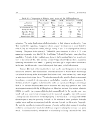
39. 1.2. Background: Structural Health Monitoring 11
modulus but with a high coupling coefficient. For those applications that can tolerate low
mechanical stiffness, PVDF is generally chosen over a piezoceramic material because of its
low modulus and relatively low cost, despite its relatively low electromechanical coupling
coefficient. Flexibility and manufacturability of PVDF sensor has made them popular
for use as thin-film contact sensors and acoustic transducers. The main advantage of
magnetostrictive sensing is that the fundamental technology is non-contact in nature so
that the sensors can last indefinitely and can be inserted inside the composite layers.
1.2.3 Solution Domain
Literature for SHM can be divided according to their solution domain. These are the
following:
1.2.3.1 Static Domain
In the presence of damage, stiffness matrix of the structure changes. Due to this change,
displacement of the structure due to static load changes. This change is one of the criteria
used for the detection of damage. Jenkins et al. [169] introduced a static deflection based
damage detection method. They mention that the other methods are relatively insensitive
to many instances of localized damage such as fatigue crack or notch, which results in very
little changes in the system mass or inertia. Zhao and Shenton [235] presented a novel
damage detection method based on best approximation of dead load stress redistribution
due to damage.
For self-equilibrating static load (usually generated from smart actuator), the effect
of load far away from the actuator has negligible effect on the static response, even in the
presence of damage. Hence, the change of structural properties distant from the actuator
cannot be sensed through static self-equilibrating load. Hence, the use of smart actuator
for SHM in static domain is limited to the proximity of actuator only.
1.2.3.2 Modal domain
Since modal parameters depend on the material property and geometry, the change in
natural frequencies, mode shape curvature etc. can be used to locate the damage in
structures without the knowledge of excitation force, when linear analysis is adequate.
The amount of the literature pertaining to the various methods for SHM based on modal
domain is quite large [58, 66, 177, 197, 197, 221, 242, 290, 342, 378, 379]. New and

40. 12 Chapter 1. Introduction
sophisticated strategies for damage identification using modal parameters is studied ex-
tensively (e.g. [Ratcliffe, [320]; Lam et al., [208]; Ratcliffe and Bagaria, [321]; Ratcliffe
[322]; Chinchalkar, [77]). Lakshminarayana and Jebaraj, [206] used the first four bending
and torsional modes and corresponding changes in natural frequencies to estimate the lo-
cation of a crack in a beam. It is reported that if the crack is located at the peak/trough
positions of the strain mode shapes, then percentage change in frequency would be higher
for corresponding modes. It is also found that if the crack is located at the nodal points of
the strain mode shapes, then the percentage change in frequency values would be lower for
corresponding modes. Uhl [376] presented different approaches for identification of modal
parameters for model-based SHM. Khoo et al. [182] presented modal analysis techniques
for locating damage in a wooden wall structure. Ching and Beck [78] used modal identifi-
cation for probabilistic SHM. Verboven et al. [378] applied total least-squares algorithms
for the estimation of modal parameters in the frequency-domain. Caccese et al. [58] stud-
ied the detection of bolt load loss in hybrid composite/metal bolted connections using
low frequency modal analysis. Sodano et al. [342] used macro-fiber composites sensor to
find modal parameters for SHM of an inflatable structure. Chan et al. [66] updated finite
element model of a large suspension steel bridge using modal characteristics for SHM of
the bridge. Laser vibrometer, designed for modal analysis was used for crack detection in
metallic structures by Leong et al. [221].
The presence of delamination changes the structural dynamic characteristics and
can be traced in natural frequencies, mode shapes, phase, dynamic strain and stress
wave patterns etc. Significant research has been reported on the effect of delamination
on natural frequencies and mode shapes and strategies have been developed to identify
location of delamination using changes in these modal parameters (Tracy and Pardoen,
[371]; Gadelrab, [127]; Schulz at al., [338]; Zou et al., [430]; Chinchalkar, [77]). Tracy and
Pardoen, [371] found that if the delamination is in a region of mode shape where the shear
force is very high, there will be considerable degradation in natural frequency, which is
otherwise not significant. Hence, by studying the mode shapes and the corresponding
natural frequencies, estimation on the location of delamination can be made.
Resonant Frequencies / Natural Frequencies: The resonant frequencies are defined
as the frequencies at which the magnitude of the frequency response at a measured de-
grees of freedom approaches infinity, which is also called as natural frequency. Adams,
et al. [4] illustrated a method to detect damage from changes in resonant frequencies.
Wang and Zhang [389] estimate the sensitivity of modal frequencies to changes in the

41. 1.2. Background: Structural Health Monitoring 13
structural stiffness parameters. Zak et al. [420] examined the changes in resonant fre-
quencies produced by closing delamination in a composite plate. In particular, the effects
of delamination length and position on changes in resonant frequencies were investigated.
Williams and Messina [396] formulate a correlation coefficient that compares changes in a
structure’s resonant frequencies with predictions based on a frequency-sensitivity model
derived from a finite element model. Hearn and Testa [152] developed a damage detection
method from ratio of changes in natural frequency for various modes.
Antiresonance frequencies: The antiresonance frequencies are defined as the frequen-
cies at which the magnitude of the frequency response at measured degrees of freedom
approaches zero [310]. To calculate antiresonance frequencies of a dynamic system, He
and Li [151] developed an accurate and efficient method for undamped systems. The rea-
sons for looking to the antiresonance frequencies are that these antiresonance frequencies
can be easily and accurately measured in a similar way as for the natural frequencies.
Furthermore, a system can have much greater number of antiresonance frequencies than
natural frequencies because every different FRF between an actuator and a sensor con-
tains another set of antiresonance frequencies. Williams and Messina [396] considered
anti-resonance frequencies for their damage detection technique. Lallement and Cogan
[207] introduced the concept of using antiresonance frequencies to update FE models.
Mottershead [275] showed that the antiresonance sensitivities to structural parameters
can be expressed as a linear combination of natural frequency and mode shape sensitivi-
ties, and furthermore that the dominating contributors to the antiresonance sensitivities
are the sensitivities of the nearest frequencies and corresponding mode shapes. It is con-
cluded that the antiresonance frequencies can be a preferred alternative to mode shape
data.
Mode Shapes: Doebling and Farrar [99] examine changes in the frequencies and
mode shapes of a bridge as a function of damage. This study focuses on estimating the
statistics of the modal parameters using Monte Carlo procedures to determine if damage
has produced a statistically significant change in the mode shapes. Stanbridge, et al. [343]
also use mode shape changes to detect saw-cut and fatigue crack damage in flat plates.
They also discuss methods of extracting those mode shapes using laser-based vibrometers.
Another application of SHM using changes in mode shapes can be found in (Ahmadian
et al. [13]). West [393] used mode shape information (Modal Assurance Criteria) for the
location of structural damage. Ettouney et al. [116] discuss a comparison of three different
SHM techniques applied to a complex structure, which are based on the information of

42. 14 Chapter 1. Introduction
mode shapes and natural frequencies of the damaged and undamaged structure.
Mode Shape Curvatures / Modal Strain Energy: Pandey, et al. [303] identified the
absolute changes in mode shape curvature as an indicator of damage. An experimental
damage detection investigation of fiber-reinforced polymer honeycomb sandwich beams
was performed by Lestari and Qiao [222] based on the curvature mode shapes. Different
damage detection algorithms were studied by Hamey et al. [143] using curvature modes of
structures with piezoelectric sensors or actuators. Ho and Ewins [157] present a Damage
Index method, which is defined as the quotient squared of a structure’s modal curvature
in the undamaged state to the structure’s corresponding modal curvature in its damaged
state. In another paper by Ho and Ewins [158], the authors state that higher derivatives
of mode shapes are more sensitive to damage, but the differentiation process enhances
the experimental variations inherent in those mode shapes. Zhang et al. [425] propose
a structural damage identification method based on element modal strain energy, which
uses measured mode shapes and modal frequencies from both damaged and undamaged
structures as well as a finite element model to locate damage. Worden et al. [403] present
another strain energy study using a damage index approach. Carrasco et al. [55] discuss
using changes in modal strain energy to locate and quantify damage within a space truss
model. Choi and Stubbs [83] used changes in local modal strain energy to develop a
method for detecting damage in two-dimensional plates.
Modal Damping: When compared to frequencies and mode shapes, damping prop-
erties have not been used as extensively as frequencies and mode shapes for damage
diagnosis. Crack detection in a structure based on damping, however, has the advantage
over other detection schemes based on frequencies and mode shapes. This is due to the
fact that the damping changes have the ability to detect the nonlinear, dissipative effects
that cracks produce. Modena et al. [272] show that the visually undetectable cracks cause
very little change in resonant frequencies and require higher mode shapes to be detected,
while the same cracks cause larger changes in the damping. Zonta et al. [429] observe that
crack creates a non-viscous dissipative mechanism for making damping more sensitive to
damage. Kawiecki [176, 177] notes that damping can be a useful damage-sensitive feature
particularly suitable for SHM of lightweight and micro-structures. Author has described
the application of arrays of surface-bonded piezo-elements to determine modal damping
characteristics for structural healthy monitoring of light-weight and micro-structures.
Dynamic Stiffness from Mode shape: Many structural health-monitoring techniques
rely on the fact that structural damage can be expressed by a reduction in stiffness. Maeck

43. 1.2. Background: Structural Health Monitoring 15
and Roeck [243] apply a direct stiffness approach to damage detection, localization, and
quantification for a bridge structure, which uses experimental frequencies and mode shapes
in deriving the dynamic stiffness of a structure.
Dynamic Flexibility from Mode shape:A reduction in stiffness corresponds to an
increase in structural flexibility. Dynamically measured flexibility matrix [G] of the dam-
aged structure can be estimated from the natural frequencies [Λ] and normalized mode
shapes [Φ] as:
[G] ≈ [Φ][Λ]−1 [Φ]T
Pandey and Biswas [302] present a damage-detection and damage localization method
based on changes in the flexibility of the structure. Mayes [261] uses measured flexibility to
locate damage from the results of a modal test on a bridge. Aoki and Byon [21] presented
modal-based structural damage detection using localized flexibility properties that can
be deduced from the experimentally determined global flexibility matrix. Bernal [39]
mentions that changes in the flexibility matrix are sometimes more desirable to monitor
than changes in the stiffness matrix. Because the flexibility matrix is dominated by the
lower modes, good approximations can be obtained even when only a few lower modes
are employed. Reich and Park [327] focus on the use of localized flexibility properties
for structural damage detection. The authors choose flexibility over stiffness for several
reasons, including the facts that (1) flexibility matrices are directly attainable through
the modes and mode shapes determined by the system identification process, (2) iterative
algorithms usually converge the fastest to high eigenvalues, and (3) in flexibility-based
methods, these eigenvalues correspond to the dominant low-frequency components in
structural vibrations. A structural flexibility partitioning technique is used because when
the global flexibility matrix is used, there is an inability to uniquely model elemental
changes in flexibility. The strain-based sub-structural flexibility matrices measured before
and after a damage event, are compared to identify the location and relative degree of
damage. Topole [368] discusses the use of the flexibility of structural elements to identify
damage. Author indicates that there are certain instances where it is advantageous to use
changes in flexibility as an indicator of damage rather than using stiffness perturbations.
Topole develops a sensitivity matrix that describes how modal parameters are affected
by changes in the flexibility of structural elements. From this information, he develops a
scalar quantity for each structural element, which indicates the relative level of damage
within the element.
Unity Check Method: In unity check method, the product of an undamaged stiffness

44. 16 Chapter 1. Introduction
matrix K u and dynamically measured flexibility matrix [G] from a unity matrix at any
stage of damage are checked using following relation.
[E] = [G][K u ] − I
The unity check method, proposed by Lin [230, 231] is useful for locating and quantifying
damage using modal parameters.
Best Achievable Eigen Vectors: Lim and Kashangaki, [229] located damage in space
truss structures by computing Euclidian distances between the measured mode shapes
and best achievable eigenvectors. The best achievable eigenvectors are the projection of
the measured mode shapes onto the subspace defined by the refined analytical model of
structure and measured frequencies.
Limitation of Modal Domain in SHM: However modal methods are not very sen-
sitive to the small size of delaminations which are of practical interest, and can be very
cumbersome as well as computationally expensive while implementing in practice for on-
line health monitoring. In most of the methods based on modal parameters, it is assumed
that the modes under consideration are affected by damages. As pointed out by Ratcliffe,
[322], the change in individual natural frequencies due to small damage may become
insignificant and may fall within measurement error. In practical situation, this can con-
siderably reduce the effectiveness of the prediction. The main limitation of modal domain
approach is that the lower modes are less sensitive to damage, particularly becomes a
significant problem when only a few lower modes are used in SHM. Change of structural
dynamic performance caused by structural damage that is less than 1% of the total struc-
tural size is unnoticeable. Yan and Yam [415] pointed out that when the crack length in
a composite plate equals 1% of the plate length, the relative variation of structural nat-
ural frequency is only about 0.01 to 0.1%. Therefore, using vibration modal parameters,
e.g., natural frequencies, displacement or strain mode shapes, and modal damping are
generally ineffective in identifying small and incipient structural damage.
1.2.3.3 Frequency Domain
In frequency domain method, most important part is to calculate the dynamic stiffness
matrix at each frequency either from stiffness and mass matrix or directly from spectral
formulation. The applied load vector is transformed in the frequency domain by Fourier
Transform, and solved for structural response at each frequency. After getting responses
for each frequency, inverse Fourier Transform gives the time domain responses.

45. 1.2. Background: Structural Health Monitoring 17
Frequency Response Function (FRF): Although the majority of investigations into
structures under dynamic loading are concerned with obtaining the natural frequencies,
and possibly mode shapes, of the structure, a much more valuable description of the
dynamic behavior of the structure is the FRF, which describes the relationship between a
local excitation force applied at one location on the structure and the resulting response
at another location. Essentially, the FRF returns information about the behavior of the
structure over a range of frequencies. The response at a particular frequency for some
forcing and response locations will simply be a single complex number, which is often
plotted in terms of real and imaginary parts or in terms of amplitude and phase. The
frequency response of a system can be measured by: (1) applying an impulse to the
system and measuring its response. (2) sweeping a constant-amplitude pure tone through
the bandwidth of interest and measuring the output level and phase shift relative to the
input.
Mal et al. [252] presented a methodology for automatic damage identification and
localization using FRF of the structure. Agneni, et al. [12] use the measured FRFs for
damage detection. Lopes, et al. [237] relate the electrical impedance of the piezoelec-
tric material to the FRFs of a structure. The FRFs are extracted from the measured
electric impedance through the electromechanical interaction of the piezoceramic and the
structure. Trendafilova [372] use the FRFs as damage-sensitive features.
Spectral finite element (SFE): SFE gives exact dynamic stiffness matrix for two
noded elements for frequency domain solution. Sreekanth et al. [198] had modeled trans-
verse crack in SFE formulation to simulate the diagnostic wave scattering in composite
beams for SHM technique. Mahapatra and Gopalakrishnan [247] had studied the effect
of wave scattering and power flow through multiple delaminations and strip inclusions in
composite beams with distributed friction at the inter-laminar region using SFE formu-
lation. Nag et al. [285] had proposed a SFE method for modeling of wave scattering in
laminated composite beam with delamination.
1.2.3.4 Time-Frequency Domain
In contrast to the Fourier analysis, the time-frequency analysis can be used to analyze
any nonstationary events localized in time domain. Vill [381] notes that there are two
basic approaches to time-frequency analysis. The first is to divide the signal into slices
in time and to analyze the frequency content of each of these slices separately. The
second approach is to first filter the signal at different frequency bands and then cut

46. 18 Chapter 1. Introduction
the frequency bands into slices in time to analyze their energy content as a function
of time and frequency. The first approach is the basic short term Fourier transform,
also known as spectrogram, and the second one is the Wigner-Wille Transform. Other
time-frequency analysis techniques include, but are not limited to, wavelet analysis and
empirical mode decomposition combined with Hilbert transform. Bonato et al. [44]
extract modal parameters from structures in non-stationary conditions or subjected to
unknown excitations using time-frequency and cross-time-frequency techniques. Mitra
and Gopalakrishnan [269, 270, 271] have developed wavelet transform based spectral finite
element formulation, which they used to identify the delamination of composite laminates.
1.2.3.5 Impedance Domain
The basic concept of impedance method is to use high-frequency structural excitations
to monitor the local area of a structure for changes in structural impedance that would
indicate imminent damage. The impedance domain technique successfully detects damage
that is located near the sensor/actuator.
Electro-mechanical impedance (EMI): Electro-mechanical impedance is a technique
for SHM that uses a collocated piezoelectric actuator/sensor to measure the variations of
mechanical impedance of a structural component or assembly. This technique relies on the
electromechanical coupling between the electrical impedance of the piezoelectric materials
and the local mechanical impedance of the structure adjacent to the PZT materials.
The PZT materials are used both to actuate the structure and to monitor the response.
From the input and output relationship of the PZT materials, the electrical impedance
is computed. When the PZT sensor actuator is bonded to a structure, the electrical
impedance is coupled with the local mechanical impedance. Small flaws in the early
stages of damage are often undetectable through global vibration signature methods,
but these flaws can be detected using the PZT sensor-actuator, provided that the PZT
sensor actuators are near the incipient damage. By inspecting the differences between the
impedance spectrum of a reference baseline of the structure in an undamaged condition
and the impedance spectrum of the same structure with damage, incipient anomalies of
the structural integrity can be detected. This health monitoring technique can also be
implemented in an on-line fashion to provide a real-time assessment to detect the presence
of structural damage.
Giurgiutiu and Zagrai [137] used high-frequency electro-mechanical impedance spec-
tra for health monitoring of thin plates. Park et al. [305] summarized the hardware

47. 1.2. Background: Structural Health Monitoring 19
and software issues of impedance-based SHM, where high-frequency structural excitations
are used to monitor the local area of a structure from changes in structural impedance.
Piezoelectric-wafer active sensors SHM and damage detection based on elastic wave prop-
agation and the Electro-Mechanical (E/M) impedance technique is reviewed by Giurgiu-
tiu et al. [138]. Giurgiutiu et al. [136] apply this method for health monitoring of
aging aerospace structures. Giurgiutiu and Rogers [135] discussed the use of an Electro-
Mechanical Impedance (EMI) technique to detect incipient damage within a structure.
Limitation of Impedance Domain: Although, Impedance technique is suitable for the
detection of very small damage, it cannot identify damage from the far field measurement.
This is due to very high frequency solution domain, which is suitable for local identification
of damage.
1.2.3.6 Time Domain
In time domain SHM, damage is estimated using time histories of the input and vibration
responses of the structure. The structure is excited by multiple actuators across a desired
frequency range. Then, the structure’s dynamics are characterized by measuring the
response between each actuator/sensor pair. Using these time response over a long period
while at the same time taking into account the information on several modes so that the
damage evaluation is not dependent on any one particular mode, the presence of damage
is assessed. The big advantage of this method is that it can detect damage situations
both globally and locally by monitoring the input frequencies. In industry, using the
time domain measured structural vibration responses to identify and monitor structural
damage is one of the important ways to ensure reliable operation and reduced maintenance
cost for in-service structures. One of the main advantages of this solution domain is, it
can handle nonlinearity and hysteresis easily.
1.2.4 Levels of SHM
The major tasks in structural health monitoring and damage identification can be cate-
gorized under different levels as given below:
1.2.4.1 Unsupervised SHM
Unsupervised SHM is defined as the one, where the structural model of damage state is
not available for computation.

48. 20 Chapter 1. Introduction
NDE: Different nondestructive testing (Visual Inspection, Thermograph, Electrical
resistance, Magnetic particle, Eddy current, Die penetration, Acoustic Emission etc.) are
used for structural health monitoring.
Novelty detection: In this level of SHM, sensor responses of both damaged and
undamaged structure are required (for same actuation) to compare healthy and damaged
structural response for identification of the existence of damage.
Material Property identification: Different material property identification (damp-
ing, elasticity, density, magneto-mechanical coupling etc.) is performed from sensor re-
sponse and actuation.
Force Identification: Actuation or Impact force identification (bird strike, space de-
bris or foam impact in space craft, aerodynamic forces etc.) requires both sensor response,
and undamaged structural model.
Damage localization: Basic idea behind damage localization is some unbalanced
forces exist near the damage. That is, if damage occurs, the damage vector will have
nonzero entities only at the DOFs connected to the damaged elements. Fukunaga et al.
[126] showed a damage identification method based on dynamic residual forces which can
be evaluated using an analytical model of undamaged structures and measured vibration
data of damaged structures. Schulz et al., [338] used damage force to identify the elements
having damage. Nag et al. [284] have used damage force indicator for identification of
delaminations in laminated composite beams with spectral finite element model based on
the Fast Fourier Transform.
1.2.4.2 Supervised SHM
Supervised SHM is defined as where structural model of damaged state is also available
for computation.
Damage confirmation: This is referred as forward problem in structural health
monitoring. Damage location and extent are assumed and modelled in finite element to get
the response of damaged structure. If this response dose not matches with experimentally
measured response, damage properties are changed. So, this is an iterative process. As
the finite element computation is costly, good prediction of damage is always required,
which can be obtained from inverse mapping between damage to its responses.
Damage estimation: This is refereed to as inverse problem in structural health
monitoring. It identifies the magnitude, location and type of the damage from response
of damaged structure directly using artificial neural network, which are trained by some

49. 1.2. Background: Structural Health Monitoring 21
responses of different assumed damage configuration.
1.2.5 Damage Modelling in Composite Laminate
Composite structures provide opportunities for weight reduction, tailoring the material,
integrating control surfaces in the form of embedded transducers etc., which are not
possible with conventional metallic structures. Therefore, a potential barrier at present is
that the composite structures can have internal defects and they are difficult to be detected
but need frequent monitoring to asses their vulnerability. Although, matrix cracking, fiber
breakage, fiber debonding etc. initiate the damage that occurs in laminated composites,
inter-laminar crack or delamination is most vulnerable and can grow, thus reducing the life
of the structure. This is because of the fact that in contrast to their in-plane properties,
transverse tensile and inter-laminar shear strengths are quite low.
Damage states in composite and their evolution is a complex process. They depend
on the geometric scale and the micro-structural properties of the material system at
the interfaces. The matrix phase of the composite shows micro-cracks in it, which are
characterized by matrix crack density. In laminated composite, such micro-cracks appear
due to fiber separation in an angle plies. Under in-plane tensile load, as well as under
bending load, these transverse micro-cracks first grow through the thickness of the layer
and reach the upper and the lower interfaces with the neighboring layers. Similar but more
complex growth occurs in inhomogeneous composite having array of cells and interfaces
in three dimensions. The micro-cracks increase in number under increasing deformation.
Due to mismatch in the elastic moduli between the neighboring layers, possibility of having
delamination is very high. As the critical value of the strain energy release rate is reached,
the delaminations start growing rapidly. As a result, under the condition of matrix crack
density being very high, which results in angle plies not able to take any tensile load,
this tensile load is then transferred through the 0◦ fibers. With further increase of tensile
loading, the 0◦ fibers break. This is the final stage of failure. Similarly, under compressive
load, the laminates start buckling at the delaminated zone and may fail instantaneously.
1.2.5.1 Matrix cracking
Matrix cracking has long been recognized as the first damage mode observed in composite
laminates under static and fatigue tensile loading. It does not necessarily result in the
immediate catastrophic failure of the laminate and therefore can be tolerated. However, its
presence causes stiffness reduction and can be detrimental to the strength of the laminate.

50. 22 Chapter 1. Introduction
It also triggers the development of delaminations, which can cause fiber-breakage in the
primary load-bearing plies. A number of theories have appeared in an attempt to predict
the initiation of transverse cracking and describe its effect on the stiffness properties of the
laminate. Following are the methods on which these theories are based: the self-consistent
method, variational principles, continuum damage mechanics, shear lag, approximate
elasticity theory solutions and stress transfer mechanics.
Modelling of cracked beams can be performed by 2-D or 3-D FEM. Alternatively;
simplified procedures are available with less computational effort. Among these simplified
methods are those proposed by Christides and Barr [86] and Shen and Pierre [339, 340].
In both cases, a crack function representing the perturbation in the stress field induced
by the crack is considered. Chondros et al. [84] have developed a continuous cracked
beam vibration theory. They considered that the crack introduces a continuous change
in the flexibility in its neighborhood and models it by incorporating a displacement field
consistent with the singularity. In other cases, the cracked beam is modelled as two
segments connected by means of massless rotational springs [4], whose stiffness may be
related to the crack length by the fracture mechanics theory [172]. Thus, at the cracked
section, a discontinuity in the rotation due to bending must be considered. These kinds
of models have been successfully applied to Euler-Bernoulli cracked beams with different
support conditions [287, 218, 28, 43, 121, 120].
Dvorak et al. [113] evaluated overall stiffnesses and compliances, for a composite
lamina which contains a given density of matrix cracks and subjected to uniform me-
chanical loads. The evaluation procedure is based on the self-consistent method and is
similar, to that used in finding elastic constants of unidirectional composites. Hashin [147]
analyzed cross-ply laminates by variational methods for tensile and for shear membrane
loading, which contain distributions of intralaminar cracks within the 90 degree ply. In an-
other paper, Hashin [148] treated the problem of stiffness reduction and stress analysis of
orthogonally cracked cross-ply laminates under uniaxial tension by the variational method
based on the principle of minimum complementary energy. Talreja [363] predicted the
stiffness reductions due to transverse cracking in composite laminates from crack initiation
to crack saturation using the stiffness-damage relationships of continuum damage model.
Later, Talreja et al. [364] tested cross ply laminate under longitudinal tensile loading for
the behavior of transverse cracking and the associated mechanical response. Shear-lag-
based models [423, 424, 155, 297, 146, 217, 409, 40, 422] remain the most commonly used
ones for calculating the reduced stiffness properties of transversally cracked composites.

51. 1.2. Background: Structural Health Monitoring 23
They are being modified and generalized to enable better description of wider classes of
laminates. Nuismer and Tan [293] gave an approximate elasticity theory solution for the
stress-strain relations of a cracked composite lamina. McCartney [263, 264] estimated the
dependence of the longitudinal values of Young’s modulus, Poisson’s ratio, and thermal
expansion coefficient on the density of transverse cracks. Recently, Kumar et al. [198, 199]
modelled cracked composite laminate using spectral finite element formulation for wave
based structural diagnostics.
1.2.5.2 Techniques for Modelling of Delamination
Delaminations in composites are usually modelled using beams, plates or shells with ap-
propriate kinematics. The technique used by Majumdar and Suryanarayana [251] to
model a through-width delamination subdivides the beam into a delamination region
(sub-laminates) and two integral regions (base-laminates) on either side of the delamina-
tion region. Each of these sub-laminates and base-laminates are modelled as Euler beam
and the whole structure is solved satisfying global boundary conditions. For one dimen-
sional beam elements, additional axial forces give rise to a net resultant internal bending
moment which creates differential stretching of the sub-laminates above and below the
plane of delamination. The model used by Tracy and Pardoen [371] to study the effect
of delamination on natural frequency is also based on the engineering beam theory. This
model uses 2-D beam elements and includes the effect of contact between the delaminated
surfaces and can allow independent extensional and bending stiffness.
Gadelrab [127] in his work has taken two different types of finite elements for the
undelaminated and delaminated elements. For undelaminated elements, all the lamina
assumed to have the same transverse and longitudinal displacements at a typical cross-
section, but each lamina can rotate by different amount from the others depending on
its material and geometrical properties. This is also called “layer-wise constant shear
kinematics”. The delaminated element has the same transverse and axial displacement
at both ends of the element. Only the rotation is different along the element length
of each lamina. In the same direction, Barbero and Reddy [29] used layer-wise plate
theory for modelling delamination in plates where delaminations were simulated by step
discontinuity at the interfaces.
Modelling performed by Luo and Hanagud [238] assumes opening and closing ac-
tion at the region of delamination. Here it is considered that after delamination, partially
intact matrix and fibers still fill the delamination gap. The contact effect between the de-

52. 24 Chapter 1. Introduction
laminated sub-laminates is modelled as a distributed nonlinear soft spring between them.
The spring is taken as nonlinear because when the delamination opens beyond some small
amplitude constraints, the spring effect becomes zero; on the other hand, when the vibra-
tion mode does not tend to open the delamination, the delaminated sub-laminates have
the same flexural displacements and slopes. This nonlinear spring is then simplified as a
combination of few linear springs. Such modelling provides better representation of the
practical problem. In many mechanical components under fatigue loading, such delami-
nation can induce non-linear modes in vibration characteristics. Related measurements
in metal beam with fatigue crack can be found in L´onard et al. [220].
e
Williams [398] has proposed a generalized theory of delaminated plates using a
global / local variation approach. This theory uses unique coupling between the global
and local displacement fields in two different length scales and is a generalization of
the earlier proposed theories based on ”layer-wise constant shear kinematics”. However,
these above global/local analysis are based on semi-analytic approach and difficult to
incorporate for transient dynamic and wave-based diagnostic problems.
In continuum mechanics, formulation for damage, one can use a mixed variational
formulation in the local coordinates to capture the localized stress field accurately. An
assumed stress field for the local damage region and assumed displacement for the global
region can generally be used (Pagano [300]). Here, one can consider an appropriate dam-
age dependent constitutive model (Coats and Harris [90]) based on continuum damage
mechanics for the local region, and equivalent fiber-matrix mixture constitutive model
(Reddy [324]) for the global region. However, such detailed model becomes computation-
ally intensive in the context of structural health monitoring and identification of damage.
Neglecting the relative rotation of the damaged and undamaged sections and treat-
ing the structures with Euler-Bernoulli or Kirchhoff type kinematics delamination models
have been verified experimentally by Purekar and Pines [315] in the context of wave prop-
agation in delaminated isotropic helicopter flexbeams, and by Luo and Hanagud [238] in
the context of natural frequency change in first order shear deformable composite beam
with delamination and the associated contact non-linearity in the low frequency dynam-
ics. Also, such simplified model can be found useful while modelling advanced composite
with stitching (Sankar and Zhu [337]) and various other types of material interfaces.
Considering axial-flexural-shear coupled wave propagation in composite beams, a
delaminated spectral element has been developed by Mahapatra [245], where the exact
dynamics of internal debonded sub-laminates was taken into account. In this formulation,

53. 1.2. Background: Structural Health Monitoring 25
the internal FE nodal informations are condensed out leaving the delamination in between
the end nodes.
The restriction due to constant shear kinematics can be eliminated using the ap-
proach reported by Barbero and Reddy [29], where the layer-wise kinematics allows indi-
vidual sub-laminates to rotate by different amount. Similar approach has been used by
Kouchakzadeh and Sekine [191], where the formulation uses penalty function to impose ap-
propriate constraints at the interface between base-laminates and multiple sub-laminates.
In the works of Lee et al., [212] and Lee [213], the interface is assumed to translate and
rotate in a rigid-body mode. Thus, the normal plane is assumed continuous across the
base laminate thickness and is hence not affected by the stress discontinuity in the two
delaminated faces at the tip due to Mode-I and Mode-II stable delaminations. However,
this assumption may not be adequate, since strong coupling between the displacement
components may exist in case of asymmetric ply stacking, asymmetry among the sub-
laminates (due to inclusions of different material) and discontinuity in the stiffness and
inertia by foreign inclusions such as MEMS devices and integrated electronics.
Mahapatra [245] used spectral finite elements to model the individual sub-laminates,
base-laminates and strip inclusions. A layer-wise constant shear kinematics was imposed
by him at the interfaces of sub-laminates and base-laminates. Equilibrium of the system
was then obtained using multi-point constraints in Fourier domain associated with the
nodal displacement components and the force components at these interfaces allows to
model small local rotations of the individual sub-laminates and the base-laminates at
the interface in an average sense. Also, the model is a general one, where the length-
wise multiple delaminations of debonding between strip inclusions can be modelled easily.
Another advantage of the model is that both the frequency domain changes in phase and
amplitude of scattered waves in presence of delaminations or strip inclusions as well as
the time domain change in the response can be computed efficiently with the help of FFT
(Mahapatra et al., [244]).
1.2.5.3 Multiple Delaminations
The delaminations usually appear in several interfaces through the thickness of the lami-
nate (multiple delaminations), between plies of different fiber angles, and are oblong in the
direction of the fibers in the lower ply interface. The area of the delaminations increases
through the thickness away from the point of impact. Multiple delamination damage
identification in a composite plate using migration technique was proposed by Wang and

54. 26 Chapter 1. Introduction
Yuan [388]. Chattopadhyay et al. [72] had studied time domain nonlinear dynamic re-
sponse of composite laminates using a refined layer-wise theory with piezoelectric sensors
and multiple delaminations, where the contact problem of delaminated interfacial surfaces
was modelled in terms of fictitious linear springs to provide an accurate description of the
transient behavior.
Mahapatra and Gopalakrishnan [247] had studied the effect of wave scattering and
power flow through multiple delaminations and strip inclusions in composite beams with
distributed friction at the inter-laminar region using spectral finite element formulation.
In this model [247], the multiple delaminated beams are divided into several sound beams
at the front of the delamination tip and the beam kinematics are then imposed. Each beam
is constrained to contact each other but a free mode assumption is generally considered
for linear analysis of the structure. Hence, each beam segment freely vibrates without
touching each other. The effect of bending-extension coupling induced from the presence
of delaminations can also be considered in the formulation.
1.2.6 Effective SHM Methodology
With the conventional NDE techniques, the complex mechanical system needs to be taken
out of service for inspection. Where as, modal domain approaches are less sensitive to the
small size damages. Small damages is sensitive to higher modes. To extract information
from higher modes smart actuator/sensor based SHM techniques are used. In very high
frequency (> 30kHz), global nature of the structure is remain unidentified. Approach in
frequency domain is suitable for linear system. Time domain approach can detect damage
with nonlinearity and hysteresis.
1.3 Background: Magnetostrictive Materials
Some magnetic materials (magnetostrictive) show elongation and contraction in the mag-
netization direction (Figure-1.1) due to an induced magnetic field. This is called the
magnetostriction, which is due to the switching of a large amount of magnetic domains
caused by spontaneous magnetization, below the Curie point of temperature. Thus mag-
netostrictive materials have the ability to convert magnetic energy into mechanical energy
and vice versa. This coupling between magnetic and mechanical energies is the transu-
dation capability that allows a magnetostrictive material to be used in both actuation
and sensing devices. Due to magnetostriction and its inverse effect (also called Villery

55. 1.3. Background: Magnetostrictive Materials 27
MAGNETIC FIELD
S N
S N
N N S S
S N
S N N
S
N N N S S S
−Hg −Hc H=0 Hc Hg
MAGNETIC FIELD
Figure 1.1: Magnetostriction due to switching of magnetic domains.
effect)[382], magnetostrictive materials can be used both as an actuator and as well as
a sensor. References [369] and [260] performed extensive work related to electrostrictive
and piezoelectric phenomena which have similarities in form with the magnetostriction
phenomena.
1.3.1 Initial History
The first positive identification of a magnetostrictive effect was in 1842 [171] when James
Joule observed that a sample of nickel changed in length when it was magnetized. Sub-
sequently, cobalt, iron and alloys of these materials were found to show a significant
magnetostrictive properties with strains of about 50 parts per million (ppm). Apart from
magnetostriction and its inverse effect, other similar phenomenon known as the Wiede-
mann effect is present in such material, which is the twisting of the material when a helical
magnetic field is applied. Its inverse effect is called the Matteuci effect [258], which is the
creation of a helical field when the same material is subjected to a torque. One of the first
practical applications of magnetostriction was its use in SONAR devices in echo location
during the Second World War. Another early application was in torque sensing and these
applications are as important today as they were then. The nickel based materials used in
these devices had saturation magnetostriction values of 50 ppm. These strains are quite
low and hence have limited applications.

56. 28 Chapter 1. Introduction
1.3.2 Rare Earth Material Era
In the 1960s, the rare-earth elements terbium (T b) and dysprosium (Dy) were found to
have 100 times the magnetostrictive strains found in nickel alloys. However, because this
property occurs only at low temperatures, applications of these materials above ambient
temperature were not possible. The addition of iron to terbium and dysprosium to form
the compounds T bF e2 and DyF e2 brought the magnetostrictive properties to room tem-
perature. These materials individually required very large magnetic fields to generate a
considerable strain, which means magnetomechanical coupling coefficient is very small.
1.3.2.1 Giant Magnetostrictive Materials
The theoretical and experimental study of magnetostrictive materials has been the focus
of considerable research for many years. However, only the recent development of gi-
ant magnetostrictive materials (e.g. Terfenol-D) has enabled to produce sufficiently large
strains and forces to facilitate the use of these materials in actuators and sensors. This has
led to the application of magnetostrictive materials to such devices as micro-positioners,
vibration controller, sonar projectors and insulators, etc. Giant magnetostrictive material
has the ability to operate at high temperatures, and they give large strain for low mag-
netic field intensity and hence have very high coupling coefficient. By alloying the two
compounds T bF e2 and DyF e2 , it was found that the magnetic field required to produce
saturated strains were considerably reduced. The resulting alloy T b.27 Dy.73 F e1.95 (com-
mercially known as Terfenol-D) is at present the most widely used giant magnetostrictive
material. Terfenol-D is capable of strains as high as 1500ppm and, since the 1980’s,
it is commercially available for applications in many fields of science and engineering.
Terfenol-D is known to have high magnetostriction and low anisotropy energy. Therefore,
comparatively high strain amplitudes, approaching 1000ppm, can be obtained at low field
(<100kA/m).
1.3.3 Applications
Due to its capacity to sense and actuate, giant magnetostrictive materials is used in
wide varieties of applications. Choudhary and Meydan [85] designed accelerometer using
inverse effect of magnetostrictive material. Oduncu and Meydan [296] performed Bio-
chemical monitoring using magnetostrictive material. They determined the stress and
strain in bone and bone implant to assess fracture healing. Hattori et al. [149] studied

57. 1.3. Background: Magnetostrictive Materials 29
low frequency elastic wave measurement using magnetostrictive material in the concrete
structure. Customary piezoelectric devices cannot produce such a low frequency elas-
tic wave efficiently. The magnetostrictive sensors have a unique characteristic such that
one can monitor stress waves without any direct physical contact. Because of this non-
contact measurement property of the sensors, these have been used in various applications
[397, 375, 184, 14, 299, 200, 201, 202, 203, 204, 205, 281, 282]. The measurement principle
of this sensor is based on the Villari effect [382]. Cho et al. [79] investigated the design
of an optimal configuration of the bias magnet assembly to maximize the voltage output
of a magnetostrictive sensor. Visone and Serpico [383] proposed a black box type hys-
teresis model for magnetostrictive materials that is constituted by suitable composition
of Preisach-like operators.
Hristoforou [161] given a review on the use of amorphous magnetostrictive wires
in delay lines for sensing applications. Christos et al. [253] developed an optimized
distributed field sensor based on magnetostrictive delay line response, suitable for NDT
purposes. Hristoforou et al. [162] demonstrated the application of magnetostrictive delay
line arrangement in thin film thickness determination, during film production.
1.3.3.1 Thin Film and MEMS
Magnetostrictive materials are very attractive for the production of microelectromechani-
cal systems (MEMS), such as micro robots, micro motors, etc. [22, 233]. Wetherhold and
Guerrero [394] studied the effects of the stress and magnetic states of magnetostrictive
multi-layered thin films for the case in which a bending strain was applied to the sub-
strate during film deposition and then released. Jain et al. [168] used the free standing
magnetostrictive thick or thin film sensor for remote query of temperature and humidity
for time-varying external magnetic field. From the oscillations at resonant frequency of
the sensor, an acoustic wave is generated, which was detected remotely from the test
area by a microphone. Gehring et al. [129] calculated the deflection for a magnetoelastic
cantilever for an arbitrary ratio of thickness of film and substrate. Grimes et al. [141]
considered magnetoelastic thin film sensors as the magnetic analog of surface acoustic
wave sensors, with the characteristic resonant frequency of the magnetoelastic sensor to
monitor the change in the response with different environmental parameters. Pasquale et
al. [307] measured the magnetic properties of a set of (T bx F e1−x ) magnetostrictive thin
films under applied stress in a cantilever configuration with complementary flux metric
and magneto-optic Kerr effect methods.

58. 30 Chapter 1. Introduction
1.3.3.2 Thick Film, Magnetostrictive Particle Composite
Kouzoudis and Grimes [98] studied the response mechanism of magnetoelastic thick-film
sensors and have shown that the characteristic resonant frequency is a function of both
pressure and the mechanical stress. Armstrong [23] presented nonlinear magnetoelastic
behavior of magnetically dilute magnetostrictive particulate composites. To get this rela-
tionship, he assumed a uniform external magnetic field, which was operated over a large
number of well-distributed, crystallographically and globally parallel ellipsoidal magne-
tostrictive particles encased in an elastic, non-magnetic composite matrix. Saito et al.
[336] investigated the decrease of magnetization in positive magnetostrictive materials.
Giurgiutiu et al. [134] presented theoretical and experimental result from the study of a
MS-tagged fiber-reinforced composite beam under bending. Lanotte et al. [209] studied
the potentiality of composite elastic magnets as novel materials for sensors and actuators.
1.3.4 Structural Applications
Subramanian [353] presented an analytical model for a simply supported symmetric lam-
inated beams embedded with magnetostrictive layers based on the higher order shear
deformation theory. Chakraborty and Tomlinson [65] investigated the suitability of trans-
ferring appreciable amounts of magnetic energy to external media using the property of
change of magnetization of a Terfenol-D rod due to an applied force under a defined pre-
stress level. Experimental investigations was also conducted on a Terfenol-D monolithic
rod under different levels of constant pre-stress to quantitatively estimate the change in
magnetic induction and measured that the change in magnetic induction is very small
compared with that for a permanent magnet. Pan and Heyliger [301] derived analytical
solutions for the cylindrical bending of multilayered, linear, and anisotropic magneto-
electro-elastic plates under simple-supported edge conditions. Magnetostrictive material
has found its way in many structural applications such as vibration control, noise control
and structural health monitoring (see Section-1.2.2.4).
1.3.4.1 Vibration and Noise Suppression
Reddy and Barbosa [326] investigated laminated composite beams containing magne-
tostrictive layers modelled as distributed parameter systems to control the vibration sup-
pression. The effect of material properties, lamination scheme and placement of the
magnetostrictive layers on vibration suppression was investigated. Nakamura et al. [286]

59. 1.4. Artificial Neural Network 31
developed an active six degrees-of-freedom micro-vibration control system using giant
magnetostrictive actuators. Pelinescu and Balachandran [309] presented analytical inves-
tigations conducted into active control of longitudinal and flexural vibrations transmitted
through a cylindrical strut fitted with piezoelectric and magnetostrictive actuators. Fenn
et al. [119] developed a vibration reduction system for the UH-60A helicopter using mag-
netostrictive actuators drive with four trailing edge flaps on each blade. Anjanappa and
Bi [19] developed an integrated model to analyze the vibration suppression capability of a
cantilever beam embedded with magnetostrictive mini actuator using the Euler-Bernoulli
beam theory and strain energy conservation principle. Anjanappa and Bi [18] also in-
vestigated the magnetostrictive mini actuator for distributed applications and further
developed theoretical framework based on two-dimensional thermal analysis modifying
the general form of constitutive equation for a magnetostrictive material to include ther-
mal effects coming from resistive heating of a coil. Qian et al. [316] investigated vibration
control for simply supported laminated composite shells with smart plies acting as sensor
and actuator layers through magnetostrictive actuation. Pradhan et al. [311] formu-
lated a theory for a laminated plate with embedded magnetostrictive layers based on the
first order shear deformation theory (FSDT) and developed its analytical solution for
simply-supported boundary conditions based on the FSDT, and the analytical solution
for simply-supported plates is based on the Navier solution approach.
The effects of the material properties of the lamina, lamination scheme, and place-
ment of the magnetostrictive layers on the vibration suppression time have been examined
by many researchers. Brennan et al. [47] demonstrated the practical viability of a non-
intrusive magnetostrictive actuator and sensor for the active control of fluid-waves in a
pipe. Zheng et al. [426] presented active and passive magnetic constrained layer damping
treatment for controlling vibration of three-layer clamped clamped beams. Mahapatra et
al. [246] used this material to suppress all the frequency gear box noise components for
active noise control in helicopter passenger cabin.
1.4 Artificial Neural Network
Studies of Artificial Neural Network (ANN) have been motivated to imitate the way that
the brain operates. Neural networks learn by example, which gathers representative data,
and then invokes training algorithms to automatically learn the structure of the data.
Neural networks, with their remarkable ability to derive meaning from complicated or

60. 32 Chapter 1. Introduction
imprecise data, can be used to extract patterns and detect trends that are too complex to
be noticed by either humans or other computer techniques. A trained neural network can
be thought of as an ”expert” in the category of information it has been given to analyze.
This expert can then be used to provide projections for new situations.
1.4.1 The Biological Inspiration
The brain is principally composed of a very large number (100,000,000,000) of neurons,
massively interconnected. Each neuron is a specialized cell which can propagate an elec-
trochemical signal. The neuron has a branching input structure (the dendrites), a cell
body, and a branching output structure (the axon). The axons of one cell connect to
the dendrites of another via a synapse. When a neuron is activated, it fires an electro-
chemical signal along the axon. This signal crosses the synapses to other neurons, which
may in turn fire. A neuron fires only if the total signal received at the cell body from
the dendrites exceeds a certain level (the firing threshold). The strength of the signal
received by a neuron (and therefore its chances of firing) critically depends on the efficacy
of the synapses. Each synapse actually contains a gap, with neurotransmitter chemicals
poised to transmit a signal across the gap. Learning occurs by changing the effectiveness
of the synapses so that the influence of one neuron on another changes. A biological neu-
ron may have as many as 10,000 different inputs, and may send its output (the presence
or absence of a short-duration spike) to many other neurons. Neurons are wired up in
a 3-dimensional pattern. Real brains, however, are orders of magnitude more complex
than any artificial neural network so far considered. Thus, from a very large number of
extremely simple processing units (each performing a weighted sum of its inputs, and
then firing a binary signal if the total input exceeds a certain level) the brain manages to
perform extremely complex tasks. Of course, there is a great deal of complexity in the
brain, but it is interesting that the artificial neural networks can achieve some remarkable
results using a model not much more complex than this.
1.4.2 The Basic Artificial Model
Neuron receives a number of inputs (either from original data, or from the output of other
neurons in the neural network). Each input comes via a connection that has a strength
(or weight); these weights correspond to synaptic efficacy in a biological neuron. Each
neuron also has a single threshold value. The weighted sum of the inputs is formed, and

61. 1.4. Artificial Neural Network 33
the threshold subtracted, to compose the activation of the neuron. The activation signal
is passed through an activation function (also known as a transfer function) to produce
the output of the neuron. If the step activation function is used (i.e., the neuron’s output
is 0 if the input is less than zero, and the output is 1 if the input is greater than or equal
to 0) then the neuron acts just like the biological neuron described earlier (subtracting
the threshold from the weighted sum and comparing with zero is equivalent to comparing
the weighted sum to the threshold). Actually, the step function is rarely used in artificial
neural networks.
1.4.3 Historical Background
McCulloch and Pitts [265] developed models of neural networks based on their under-
standing of neurology in 1943 and shown that an artificial neural network, in theory,
could compute any mathematical or logical function. Neural network research was then
continued by Hebb [153], who proposed a mechanism for learning in biological neurons.
These models made several assumptions about how neurons worked. In 1958 Rosenblatt
[333] designed and developed the perceptron and demonstrated the ability of a perceptron
network to recognize different patterns. The perceptron had three layers with the middle
layer known as the association layer. This system could learn to connect or associate a
given input to a random output unit. Another system was the ADALINE (ADAptive
LINear Element), which was developed in 1960 by Widrow and Hoff [395]. The method
used for learning was different to that of the Perceptron; it employed the Least-Mean-
Squares (LMS) learning rule. Widrow-Hoff learning algorithm is that of gradient descent
algorithm, aimed at minimizing the error of the network.
Though, between 1960 and 1980 interest in neural networks dropped because of lack
of new ideas and computational power, in 1972 Kohonen [188, 189] and Anderson [15]
independently and separately developed new neural networks, which were able to act as
memories. In 1982, Hopfield [160] introduced a new type of network. Since the 1980s,
with the help of new personal computers and workstations, neural network development
and research has dramatically increased. One of the most important developments during
this time was the introduction of the backpropagation algorithm developed by Rumelhart
et al. [334].

62. 34 Chapter 1. Introduction
1.4.4 Neural Network Types
Neural Network types can be classified based on following attributes:
1.4.4.1 Topology
1. Single layer: A single layer network is a simple structure consisting of m neurons
each having n inputs. The system performs a mapping from the n-dimensional input
space to the m-dimensional output space. To train the network, the same learning
algorithms as for a single neuron can be used. This type of network is widely used
for linear separable problems, but like a neuron, single layer network are not capable
of classifying non linear separable data sets. One way to tackle this problem is to
use a multi-layer network architecture.
2. Multi layer: Multi-layer networks solve the classification problem for non linear
sets by employing hidden layers, whose neurons are not directly connected to the
output. The additional hidden layers can be interpreted geometrically as additional
hyper-planes, which enhance the separation capacity of the network. Figure-1.2
shows a typical multi-layer network architecture. This new architecture introduces
a new question: how to train the hidden units for which the desired output is not
known? The Back-propagation algorithm offers a solution to this problem, which is
discussed in Section-1.4.6.
1.4.4.2 Connection Type
1. Feed-forward: In computing, feed-forward normally refers to a multi-layer percep-
tron network in which the outputs from all neurons go to following but not preceding
layers, so there are no feedback loops.
2. Feedback: A feedback network is a system where the outputs are fed back into the
system as inputs, increasing or decreasing effects.
1.4.4.3 Learning Methods
There are three major learning paradigms, each corresponding to a particular abstract
learning task.
1. Supervised: In supervised training, both the inputs and the outputs are provided.
The network then processes the inputs and compares its resulting outputs against

63. 1.4. Artificial Neural Network 35
the desired outputs. Errors are then calculated, causing the system to adjust the
weights which control the network.
2. Unsupervised: In unsupervised training, the network is provided with inputs but
not with the desired outputs. The system itself must then decide what features it
will use to group the input data. This is often referred to as self-organization or
adaption.
3. Reinforcement learning: In the reinforcement learning model, an agent is connected
to its environment via perception and action.
1.4.4.4 Applications
1. Classification: Neural networks can be used successfully for pattern recognition and
classification on data sets of realistic size. Commercially important examples are
classification of fingerprints and hand printed characters.
2. Clustering: Clustering could be defined as ”the process of organizing objects into
groups whose members are similar in some way.” Clustering can be considered the
most important unsupervised learning problem
3. Function approximation: ANN can be used to approximate a function.
4. Prediction: Different series predictions can be performed by ANN.
1.4.5 Multi Layer Perceptrons (MLP)
The Multi-layer perceptron (MLP) is the most widely used type of neural network. It is
both simple and based on solid mathematical grounds. An MLP is a network of simple
neurons called perceptrons. The basic concept of a single perceptron was introduced by
Rosenblatt [333] in 1958. The perceptron computes a single output from multiple real-
valued inputs by forming a linear combination according to its input weights and then
possibly putting the output through some nonlinear activation function. Mathematically
this can be written as
n
y = ϕ( wi xi + b) = ϕ(wT x + b)
i=1
where w denotes the vector of weights, x is the vector of inputs, b is the bias and ϕ is the
activation function. The original Rosenblatt’s perceptron used a Heaviside step function as

64. 36 Chapter 1. Introduction
the activation function ϕ. Nowadays, and especially in multilayer networks, the activation
function is often chosen to be the logistic sigmoid 1/(1 + e−x ) or the hyperbolic tangent
tanh(x). These functions are used because they are mathematically convenient and are
close to linear near origin while saturating rather quickly when getting away from the
origin. This allows MLP networks to model well both strongly and mildly nonlinear
mappings.
A single perceptron is not very useful because of its limited mapping ability. No
matter what the activation function is used, the perceptron is only able to represent a
simple function. The perceptrons can, however, be used as building blocks of a larger,
much more practical structure. A typical MLP network consists of a set of source nodes
forming the input layer, one or more hidden layers of computation nodes, and an output
layer of nodes. The input signal propagates through the network layer-by-layer. It maps
an input vector from one space to another. The mapping is not specified, but is learned.
The learning process is used to determine proper interconnection weights and the net-
work is trained to make proper associations between the inputs and their corresponding
outputs. The signal-flow of such a network with one hidden layer is shown in Figure-1.2.
Mathematically this can be written as
y = ϕ3 W3 T ϕ2 W2 T ϕ1 W1 T x + b1 + b2 + b3 (1.1)
where Wi , bi and ϕi are weight matrices, bias vectors and the activation functions for ith
layer, respectively. Through this simple structure, MLP have been shown to be able to
approximate most continuous functions to very high degrees of accuracy, by choice of an
appropriate number of units and connection structure. A three-layer network (Figure-1.2)
with the sigmoidal activation functions can approximate any smooth mapping.
The MLP network can also be used for unsupervised learning by using the so called
auto-associative structure. This is done by setting the same values for both the inputs
and the outputs of the network. The extracted sources emerge from the values of the
hidden neurons. This approach is computationally rather intensive. The MLP network
needs to have at least three hidden layers for any reasonable representation and training
such a network is a time consuming process.
1.4.5.1 Transfer / Activation Function
The behavior of an MLP depends on both the weights (bias included) and the input-
output function (transfer function) that is specified for the units. This function typically

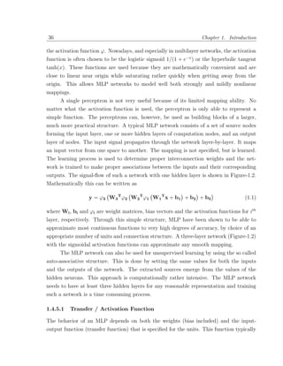
65. 1.4. Artificial Neural Network 37
falls into one of four categories:
1. Linear (or ramp): For linear units, the output activity is proportional to the total
weighted output.
2. Threshold: For threshold units, the output are set at one of the two levels, depending
on whether the total input is greater than or less than some threshold value.
3. Logistic sigmoid (1/(1 + e−x )): For sigmoid units, the output varies continuously
but not linearly as the input changes.
4. Hyperbolic tangent (tanh(x)): Logistic sigmoid and hyperbolic tangent are related
by (tanh(x) + 1)/2 = 1/(1 + e−2x ).
1.4.6 The Back-propagation Algorithm
The supervised learning problem of the MLP can be solved with the Back-Propagation
(BP) algorithm. While, there are a large number of ANN types and architectures, neural
mapping is generally been associated with the so-called back propagation network (Rumel-
hart et al. [334]). This network, in general, is organized in three types of layers: an input
layer, some hidden layers and an output layer. The algorithm consists of two steps. In
the forward pass, the predicted outputs corresponding to the given inputs are evaluated
as in Equation-(1.1). In the backward pass, partial derivatives of the error with respect
to the different parameters are propagated back through the network. The chain rule of
differentiation gives very similar computational rules for the backward pass as the ones
in the forward pass. The network weights can then be adapted using any gradient-based
optimization algorithm. The whole process is iterated until the weights have converged.
The structure of a network is determined by a number of factors including the nature
of the data to be mapped. For instance, there is usually an input unit for each input
variable and an output for each output variable of the data. The number of hidden units
(and layers) is typically determined experimentally on the basis of training results.
1.4.6.1 Training of BP ANN
The training of a BP neural network is a two-step procedure [334]. In the first step, the
network propagates input through each layer until an output is generated. The error
between the output and the target output is then computed. In the second step, the

66. 38 Chapter 1. Introduction
Output
Input
Input Layer Output Layer
Hidden Layer
Figure 1.2: Artificial Neural Network of 7-14-7 Architecture.
calculated error is transmitted backwards from the output layer and the weights are
adjusted to minimize the error. The training process is terminated when the error is
sufficiently small for all training samples. In practical applications of the back-propagation
algorithm, learning is the result from many presentations of these training examples to
the multi-layer perceptron. One complete presentation of the entire training set during
the learning process is called an epoch. The learning process is maintained on an epoch-
by-epoch basic until the synaptic weights and bias levels of the network stabilizes and the
averaged squared error over the entire training set converges to some minimum value. For
a given training set, back-propagation learning can be done in sequential or batch modes,
which are explained below.

67. 1.4. Artificial Neural Network 39
1.4.6.2 Sequential Mode
The sequential mode of back-propagation learning is also referred to as on-line, pattern,
or stochastic mode. In this mode of operation, weight updating is performed after the
presentation of each training examples. To be specific, the first example in the epoch
is presented to the network, and the sequence of forward and backward computation is
performed, resulting in a certain adjustments to the synaptic weights and the bias levels
of the network. Then the second example in the epoch is presented, and the sequence of
forward and backward computation is repeated, resulting in further adjustments to the
synaptic weights and bias levels. This process is continued until the last example in the
epoch is accounted for. It is a good practice to randomize the order of presentation of
training examples from one epoch to the next. This randomization tends to make the
search in weight space stochastic over the learning cycles, thus avoiding the possibility of
limit cycles in the evolution of the synaptic weight vectors.
1.4.6.3 Batch Mode
In this mode of back-propagation learning, weight updating is performed after the pre-
sentation of all the training examples that constitute an epoch, so that the randomization
of the training examples is of no use in this training mode. It requires local storage of
the each synaptic connection. Moreover, the network may trap in a local minimum. One
advantage of batch mode over sequential mode is that it is easier to parallelize the entire
operation.
1.4.6.4 Validation of Trained Network
To test the trained network, the data set is separated into two parts, one for training
and the other for testing the network performance. The network will be trained using
training sample and the trained network will be validated with the test sample. A network
is said to generalize well when the input-output mapping computed by the network, is
corrected with the test data that was never used in creating or training the network.
Although the network performs useful interpolation, because of multilayered perceptrons
with continuous activation functions, it leads to output functions that are also continuous.

68. 40 Chapter 1. Introduction
1.4.6.5 Execution of Trained Network
Once the network is trained and validated with sample set, it can execute rapidly to map
any point in input space to the corresponding point of output space.
1.4.7 Applications for Neural Networks
Neural networks have seen an explosion of interest over the last few years, and are being
successfully applied across an extraordinary long range of problem domains, in areas
as diverse as finance, medicine, engineering, geology and physics. Indeed, anywhere,
where there are problems of prediction, classification or control, neural networks are being
introduced. Since neural networks are best at identifying patterns or trends in data, they
are well suited for
• sales forecasting, industrial process control, customer research, data validation, risk
management, target marketing, resource allocation and scheduling, credit evaluation
(mortgage screening), investment analysis (to attempt to predict the movement of
stocks currencies etc., from previous data);
• signature analysis (as a mechanism for comparing signatures made with those stored);
recognition of speakers in communications, interpretation of multi-meaning Chinese
words, three-dimensional object recognition, hand-written word recognition, and
facial recognition;
• diagnosis of hepatitis, modelling parts of the human body and recognizing diseases
from various scans (e.g. cardiograms, scans, etc.), sensor fusion, implementation
of electronic noses (potential applications in telemedicine), instant physician (an
auto-associative memory neural network to store a large number of medical records,
each of which includes information on symptoms, diagnosis, and treatment for a
particular case);
• recovery of telecommunications from faulty software, undersea mine detection; tex-
ture analysis, monitoring the state of aircraft and diesel engines, etc.
In this thesis, the use of ANN will be explored for damage detection in compos-
ite structures, where these networks are trained using the surrogate experimental data
obtained through finite element simulation.

69. 1.5. Objectives and Organization of the Thesis 41
1.5 Objectives and Organization of the Thesis
Based on the literature survey in the previous sections, the requirements in the compu-
tational aspects of structural health monitoring using magnetostrictive materials and the
current status of the SHM, the main objectives of this thesis are
1. Develop linear and non-linear constitutive relationships of magnetostrictive materi-
als useful for structural applications.
2. Using the above developed constitutive relationships, formulate finite elements for
both coupled and uncoupled analysis.
3. Develop superconvergent and spectral finite element formulation for analysis of beam
with magnetostrictive materials.
4. Develop artificial neural network as a tool to solve inverse problem.
5. Develop higher order beams finite element with magnetostrictive sensor and actua-
tor.
6. Demonstrate the ability of the developed finite element and spectral element meth-
ods for the solution of inverse problems, such as, force and material property iden-
tification using magnetostrictive sensors.
7. Development of 2-D and 3-D elements for analysis of structure with magnetostrictive
patches.
8. Study the effect of delamination or multiple delaminations on the sensor response
due to known actuation in the beam and plate like structure.
9. Study the geometric inverse problem like delamination identification using artificial
neural network.
Thus, we have three main goals to pursue in this study. The first one is to obtain
the coupled, uncoupled, linear and nonlinear properties of the magnetostrictive material,
applicable to structural applications. The second one is to develop 1D, 2D and 3D finite
element formulation to get sensor response from known material properties and actuation
current. The third one is identification of the material properties, impact force and size
and location of delamination from magnetostrictive sensor response.

70. 42 Chapter 1. Introduction
We proceed to our study by dividing it into following three parts. In the first part,
we begin by formulating linear, nonlinear, coupled and uncoupled constitutive relation-
ships from published experimental results. All the details of formulation and numerical
examples are given in Chapter 2.
In the second part, we develop the 1D, 2D and 3D finite element formulation to
model elastic coupled and uncoupled thermo-magneto-elastic analysis (Chapter 3, Chap-
ter 4 and Chapter 5).
In the third part, structural health monitoring using magnetostrictive material as
sensors and actuators are addressed (Chapter 6 and Chapter 7). Impact force identi-
fication from sensor response is demonstrated using spectral finite element formulation
(Chapter 5). Sensor responses are used to train the artificial neural network for mate-
rial properties identification (Chapter 4) and identification of the location and size of
delamination in a structure.

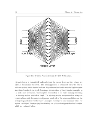
71. Chapter 2
Constitutive relationship of
Magnetostrictive Materials
2.1 Introduction
Constitutive relationship of magnetostrictive materials consists of a sensing and an actua-
tion equation. In sensing equation magnetic flux density is a function of applied magnetic
field and stress, and in actuation equation, strain is function of applied magnetic field and
stress. Both sensing and actuation equations are coupled through magneto-mechanical
coupling coefficient. Hence, to obtain the correct constitutive law of this material, both
equations need to be solved simultaneously. This chapter gives the complete details of
the numerical characterization of constitutive relations of magnetostrictive material such
as Terfenol-D.
2.1.1 Existing Literature
Existing literature in this particular area is limited. However, there are some works
that are very relevant, which is used in this chapter for the constitutive model develop-
ment. Anjanappa and Wu [17] developed a mathematical model for a magnetostrictive
particulate actuator based on the magnetoelastic material property. Ackerman et al.
[3] developed an analytical approach for formulation of input-output representations for
magnetostrictive actuators through the application of an impedance modelling method,
which included the mechanical dynamics and the electro-magneto-mechanical interaction
of the actuator device. Anhysteretic nonlinear constitutive relationships was studied by
Krishna Murty et al. [192], where the magnetostriction was considered as fourth order
polynomial of applied magnetic field for different stress level. Dapino et al. [95] mod-
elled the strains and forces generated by magnetostrictive transducers considering both
43

72. 44 Chapter 2. Constitutive relationship of Magnetostrictive Materials
the rotation of magnetic moments and the elastic vibrations in the transducer. Waki-
waka et al. [384] studied the effect of the magnetic bias for which largest linear range
was available depending on each pre-stress level. Kannan and Dasgupta [174] developed
quasi-static Galerkin finite-element theory for modelling magneto-mechanical interactions
at the macroscopic level considering body forces and coupled constitutive nonlinearities.
Kondo [190] examined the dynamic behavior of giant magnetostrictive materials.
2.1.1.1 Coupling between Actuation and Sensing Equations
Analysis of smart structures using magnetostrictive materials are generally performed us-
ing uncoupled models. Uncoupled models are based on the assumption that the magnetic
field within the magnetostrictive material is proportional to the electric coil current times
the number of coil turn per unit length (coil constant). Due to this assumption, actuation
and sensing equations gets uncoupled. For an actuator, the strain due to magnetic field
(which is proportional to coil current) is incorporated as the equivalent nodal load in the
finite element model for calculating the block force. Thus, with this procedure, analysis is
carried out without taking smart degrees of freedom in the finite element model. Similarly
for a sensor, where generally coil current is assumed zero, the magnetic flux density is
proportional to mechanical stress, which can be calculated from the finite element results
through post-processing. This assumption on magnetic field, leads to the violation of flux
line continuity, which is one of the four Maxwell’s equations in electromagnetism. To sat-
isfy Maxwell equation of flux conservation and the associated constitutive relationships,
the magnetic field should become a function of mechanical condition of the material and
this is called coupled formulation.
The constitutive model for a magnetostrictive material is essentially a coupled one.
That is, the strains and magnetic flux density are developed due to both mechanical
stress and magnetic field intensity. In coupled model, it is considered that magnetic flux
density and/or strain of the material are functions of stress and magnetic field, without
any additional assumption on magnetic field, unlike the uncoupled model. Benbouzid
et al. modelled the static [34] and dynamic [36] behavior of the nonlinear magneto-
elastic medium for magneto-static case using finite element method. Magneto-mechanical
coupling was incorporated considering both permeability and elastic modulus as functions
of stress and magnetic field. However, all these works do not provide a convenient way
for analysis of magnetostrictive smart structure, when the coupling feature is considered.
In this chapter, coupled features of magnetostrictive materials are used in a finite element

73. 2.1. Introduction 45
formulation, which has both magnetic and mechanical degrees as unknown degrees of
freedom. In addition, it is shown that the magnetic field is not proportional of applied
coil current (which is the assumption of the uncoupled model), and it depends on the
mechanical stress on the magnetostrictive material. This chapter also shows that the
coupled model preserve the flux line continuity, which is one of the drawback of uncoupled
model.
2.1.1.2 Nonlinearity of Magnetostrictive Materials
The constitutive relations of magnetostrictive materials are essentially nonlinear [52]. The
prediction of behavior of magnetostrictive material, in general, is extremely complicated
due to its hysteretic non-linear character. In structural application, due to these nonlinear
material properties, modelling of the system will also become nonlinear. Hence to model
the exact nonlinear behavior of the structure, modelling of these nonlinear properties of
magnetostrictive materials is essential.
Magnetostriction, which is the strain due to magnetic field, is a nonlinear function
of applied magnetic field. At low value of magnetic field, the slope of the curve is low,
while at medium value of magnetic field, the slope is high and again at high magnetic
field levels, the slope becomes low [52]. In addition, these magnetic field-magnetostriction
curves are different for different compressive stress level. Hence, nonlinear modelling of
magnetostriction in terms of prestress level and applied magnetic field is a difficult task.
However, the nonlinear representation of permeability in terms of magnetic field and
stress level is addressable. Also, the strain always remains positive for either positive or
negative applied field for positive magnetostriction. Therefore, the vibration frequency
will be twice that of the magnetic field if the magnetostrictive material is subjected to an
alternating current. This is the so-called double frequency effect. However, this double
frequency effect in actuation equation is generally bypassed using bias current to keep the
coil current always positive.
Traditionally, the nonlinear behavior of magnetostrictive material is studied using
uncoupled model. In uncoupled model, nonlinear actuation and sensing properties are
examined separately. For actuation, the magnetostriction for different stress level at
a particular applied magnetic field is studied. Similarly, for sensing application, the
generated magnetic flux density for different applied stress levels, are studied. Earlier
study to model uncoupled nonlinear actuation of magnetostrictive material was done in
reference [192] by considering a fourth order polynomial of magnetic field for each stress

74. 46 Chapter 2. Constitutive relationship of Magnetostrictive Materials
level. In this approach, stress level for which curve is not available, the coefficients of the
curve will have to be interpolated from the coefficients of nearest upper and lower stress
level curves. Similar approach is used in this chapter to study the nonlinear behavior of
both coupled and uncoupled formulation. In this chapter, this nonlinear representation is
modelled using different techniques such as, polynomial curve fitting and artificial neural
network.
2.1.1.3 Hysteresis of Magnetostrictive Materials
Hysteresis behavior of magnetic material can be described by a curve having three parts.
First part represents the linear material behavior, the second part represents non-linear
material behavior including saturation, and the third part describes hysteresis effects like
remanence, coercivity, static losses and accommodation. The first analytic model of fer-
romagnetic hysteresis was proposed by Rayleigh [323]. Adly, and Hafiz, [7] constructed
and identified hysteresis of magnetostriction using Preisach-type model through experi-
mental training data to a modular discrete Hopfield neural network–linear neural network
combination. Calkins, et al. [53] addresses the modelling of hysteresis in magnetostrictive
transducers based on the Jiles-Atherton mean field model for ferromagnetic hysteresis
in combination with a quadratic moment rotation model for magnetostriction. Adly, et
al. [11] presented an approach for simulating 1-D magnetostriction using 2-D anisotropic
Preisach-type models, where measured flux density versus field and strain versus field
curves for different stress values was taken into account for identification of the model.
Adly, and Hafiz, [8] proposed that artificial neural network be used as a tool to accomplish
the identification task of classical Preisach model, where the congruency property is not
exactly valid and hence required more appropriate experimental data during the identifica-
tion stage to improve the model accuracy. Adly, and Mayergoyz, [9] presented anisotropic
vector Preisach-type hysteresis models of magnetostrictive material for simulating field-
stress effects on magnetic materials. Adly, et al. [10] suggested an identification process of
two-dimensional Preisach model for modelling of one-dimensional magnetostriction using
neural network. Debruyne, et al. [96] proposed a method to characterize the Preisach
model of hysteresis phenomenon of magnetic material by taking a normal distribution law
for the switching field density. Benabou, et al. [33] presented and implemented in a finite
element code, Preisach and the Jiles-Atherton (J-A) models of hysteresis and compared
these models in terms of accuracy, numerical implementation and computational effort.
Yu, et al. [417] presented the rate-dependent hysteresis property by introducing the de-

75. 2.1. Introduction 47
pendence of the Preisach function on the input variation rate to adjust the relationship
of hysteresis loop on the input variation rate for different hysteresis systems. Cheng,
et al. [76] proposed a dynamic model which considers the eddy current, hysteresis and
anomalous losses based on Preisach modelling. Ktena, et al. [193] used a least-squares
parameter fitting procedure for one-dimensional (1D) and two-dimensional (2D) formu-
lations of the Preisach hysteresis in ferromagnets, and shape memory alloys. Ktena, et
al. [194] identified hysteresis using data from a major hysteresis curve and a least-squares
error minimization procedure for the parameters of the characteristic density. Dupre, et
al. [112] modelled the hysteresis of material like the SiFe-alloys using the Preisach theory,
took the magnetization as input to the model. Natale, et al. [288] proposed the identi-
fication and compensation of the hysteretic behavior of Terfenol-D actuator by applying
the classical Preisach model, whose identification procedure is performed by adopting of
both a fuzzy approximator and a feed-forward neural network. Ragusa [318] presented an
analytical computation of the factorized distribution function by moving Preisach model
starting from a set of measured symmetrical loops. A probabilistic model for magne-
tostrictive and magnetic hysteresis in Terfenol-D compounds is proposed by Armstrong
[24]. The critical stresses that eliminate hysteresis in magnetostrictive materials were de-
termined by Cullen et al. [93] for coherent magnetization reversal. From these works, it
can be concluded that the prediction of behavior of magnetostrictive material, in general,
is extremely complicated due to its hysteretic non-linear character.
The main goal of this chapter is to numerically characterize the constitutive model of
the magnetostrictive material for its use in structural health monitoring applications. One
of the main issues in the design of these magnetostrictive sensors/actuators is to predict
its behavior under various mechanical and/or magnetic excitation conditions through
the constitutive relationship of material. Anhysteretic sensing and actuation properties
of magnetostrictive materials (Terfenol-D) are taken into consideration in the structural
analysis for singled valued sensing and actuation. Hence only anhysteretic models of
magnetostrictive material are studied in this chapter.
The chapter is organized as follows. In Section-2.2, uncoupled formulation is de-
veloped for magnetostrictive materials. The anhysteretic modelling of magnetostrictive
material for linear-uncoupled and nonlinear-uncoupled constitutive relationships is given.
Subsequently, coupled formulations for both linear and nonlinear are given in Section-2.3
for magnetostrictive materials. For both linear and nonlinear models, total mechanical
and magnetic energy is calculated for a magnetostrictive rod. Hamiltonian principle is

76. 48 Chapter 2. Constitutive relationship of Magnetostrictive Materials
used to get the equations for magnetic and mechanical degrees of freedoms. Nonlinear
modelling of magnetostrictive material is studied with polynomial approach as well as
ANN approach. Finally, the findings of this chapter are summarized in Section-2.4.
2.2 Uncoupled Constitutive Model
Application of magnetic field causes strain in the magnetostrictive material (Terfenol-D)
and hence the stress, which changes magnetization of the material. As described by Butler
[52], Moffett et al [273], and Hall and Flatau [142], the three-dimensional linear coupling
constitutive relationship between magnetic and mechanical quantities for magnetostrictive
material are given by
{ } = [S (H) ]{σ} + [d]T {H} (2.1)
{B} = [µ(σ) ]{H} + [d]{σ} (2.2)
where { } and {σ} are strain and stress respectively. [S(H) ] represents elastic com-
pliance measured at constant {H} and [µ(σ) ] represents the permeability measured at
constant stress {σ} . Here [d] is the magneto-mechanical coupling coefficient, which pro-
vides a measure of the coupling between the mechanical strain and magnetic field. In
general, [S], [d] and [µσ ] are nonlinear as they depend upon {σ} and {H}. However,
reasonable response estimation can be obtained by treating them as linear [52].
Equation-(2.2) is often referred to as the converse effect and Equation-(2.1) is known
as the direct effect. These equations are traditionally used for sensing and actuation
purpose. It should be noted that the elastic constants used correspond to the fixed
magnetic field values and the permeability correspond the fixed stress values. Here we
propose to use an ANN model to characterize the constitutive model and compare the
solution with the reference [192].
Here the experimental data for training of ANN, is taken from Etrema manual [52]
for Terfenol-D, a giant magnetostrictive material. Experimental data given in the manual
for two different set of curves, namely the of magnetostriction - magnetic field variation for
different stress level is shown in Figure-2.1 and Figure-2.2, and the stress - strain curves
for different magnetic field levels is shown in Figure-2.3 and Figure-2.4. Here uncoupled
constitutive relationship of magnetostrictive material is considered for the study. Anal-
ysis of smart structures using magnetostrictive materials as either sensors or actuators
has traditionally been performed using uncoupled models. Uncoupled models make the
assumption that the magnetic field within the magnetostrictive material is constant and

77. 2.2. Uncoupled Constitutive Model 49
x 10
−3 Magnetostriction for Different Stress Level
1.4
1.2
1
Magnetostriction
0.8
0.6
0.4
6.9 MPa
9.6
12.4
0.2 15.1
17.9
20.7
24.1
0
0 2 4 6 8 10 12
Magnetic Field (Amp/m) x 10
4
Figure 2.1: Magnetostriction vs. magnetic field supplied by Etrema
proportional to the product of electric coil current and the number of coil turn per unit
length. Magnetostriction λ = [d]T {H} is the strain due to magnetic field, which is the
second term in the Equation-(2.1). Hence, the strain induced by an actuator and the
magnetic flux density output of a sensor, are described by two uncoupled equation. This
makes analysis of a smart structure relatively simpler. For this uncoupled model, both
linear and nonlinear analysis is performed. In the linear model, the magnetomechanical-
coupling term is assumed as constant. But generally it is a nonlinear function of magnetic
field and stress level. In the nonlinear model, the magnetostriction is modelled with a
three layer artificial neural network as it can approximate any nonlinear input-output
relationships through its universal approximation theorem [150].
From experimental data [52], only longitudinal component of magnetostriction due

78. 50 Chapter 2. Constitutive relationship of Magnetostrictive Materials
x 10
−8 Magneto−mech. Coupling for Diff Stress
3.5
6.9 MPa
9.6
12.4
3 15.1
Magneto−mechanical coupling (m/amp)
17.9
20.7
24.1
2.5
2
1.5
1
0.5
0
0 2 4 6 8 10 12
Magnetic Field (Amp/m) x 10
4
Figure 2.2: Magneto-mechanical coupling vs. magnetic field supplied by Etrema
to longitudinally applied magnetic field is present, and hence only d33 component is avail-
able. Magnetostriction in this experiment is d33 H3 . All other component of [d] matrix is
considered equal to zero. In the absence of sensing experimental data, where an applica-
tion of magnetic field and stress will produce magnetic flux form magnetostrictive sensor
(due it its inverse magnetostrictive effect, Villery Effect), sensing equation is not studied
here. In addition, actuation data for tensile stress level is also not available in the manual.
2.2.1 Linear Uncoupled Model
Although magnetostriction is highly nonlinear with magnetic field and stress, sometimes
the linear actuation model is quite sufficient especially in vibration and noise control ap-
plication. To get the linear actuation from this highly nonlinear property, some magnetic

79. 2.2. Uncoupled Constitutive Model 51
x 10
7 Stress vs. Strain for Bias fields.
14
0 Oe
100 Oe
200 Oe
12 300 Oe
400 Oe
500 Oe
600 Oe
700 Oe
10 800 Oe
900 Oe
1000 Oe
1200 Oe
Stress (Pa)
8 1500 Oe
6
4
2
0
0 0.5 1 1.5 2 2.5 3 3.5
Strain x 10
−3
Figure 2.3: Stress vs. strain relationship for different magnetic field level [Etrema]
x 10
10 Stress vs. strain Curves for Bias Fields.
10
9
8
7
Modulus (Pa)
6
5
0 Oe
4 100 Oe
200 Oe
300 Oe
3 400 Oe
500 Oe
600 Oe
2 700 Oe
800 Oe
900 Oe
1 1000 Oe
1200 Oe
1500 Oe
0
0 0.5 1 1.5 2 2.5 3 3.5
Strain x 10
−3
Figure 2.4: Elasticity vs. strain relationship for different magnetic field level [Etrema]

80. 52 Chapter 2. Constitutive relationship of Magnetostrictive Materials
and mechanical bias is used, which will shift the starting point of curves in the middle of
linear range. Hence, there is a necessity for calculation of optimum values of bias mag-
netic field and bias stress to give maximum linear range of actuation and maximum value
of tangential coupling coefficient [384]. This is a multi objective optimization problem
where maximum range of linearity as well as tangential coupling coefficient is required.
In addition, minimization of bias magnetic field and bias stress level may be other design
criteria. If permanent magnets are used for bias magnetic field, energy requirement for
constant DC current will not be required.
2.2.1.1 Actuator Design - Some Issues
It is described that the designed actuator are required to satisfy the following two consid-
eration; one, it has to behave as linear as possible, and the second; it should be efficient.
The issues relating to these two criteria are discussed below.
2.2.1.2 Linearity
Figure-2.5 and Figure-2.6 give the variation of tangential coupling and coupling coefficient
with the bias field obtained by polynomial fitting of experimental data [52], and it is shown
that for 15.1 MPa bias stress level, the linear range of actuator is from 0 to 40kA/m with
tangential coupling value 2e-8 m/amp, and for 24.1 MPa bias stress linear range is from
50 to 70kAmp/m with tangential coupling value 1.8e-8 m/Amp. Hence, 15.1 MPa stress
bias with 30 kA/m bias magnetic field is the optimal value for having higher tangential
coupling. But in general for any application, the stress level of actuator will not be
constant and hence this study will not be effective if the stress level changes.
2.2.1.3 Efficiency
The efficiency of actuator is defined as the ratio of mechanical energy to the magnetic
energy. Hence, the increased value of magneto-mechanical coupling coefficient will increase
the efficiency of actuator. Considering bias magnetic field will be obtained by a permanent
magnet, the optimum bias magnet required for higher efficiency of actuator will simply be
equal to the average magneto-mechanical coupling coefficient. The optimum value of bias
magnetic field for the average magneto-mechanical coupling coefficient is given in Figure-
2.6. Here, the average magneto-mechanical coupling coefficient is calculated for different
stress level and different bias magnetic field. It is shown that for low stressed actuator,
low strength bias magnet is optimum, while as for high stressed actuator, high strength

81. 2.2. Uncoupled Constitutive Model 53
x 10
−8 Tangential Coupling for Diff Stress
6
6.9 MPa
9.6
12.4
Magneto−mech. Tengential Coupling (m/amp)
5 15.1
17.9
20.7
24.1
4
3
2
1
0
−1
0 2 4 6 8 10 12
Magnetic Field (Amp/m) x 10
4
Figure 2.5: Tangential coupling with bias field for different stress level.
x 10
−8 Magneto−mech Coupling with Bias Magnet
2.4
6.9 MPa
9.6
2.2 12.4
Average Magneto−mech Coefficient (m/amp)
15.1
17.9
2
20.7
24.1
Average
1.8
1.6
1.4
1.2
1
0.8
0.6
0.4
0 2 4 6 8 10 12
Bias Magnetic Field (Amp/m) x 10
4
Figure 2.6: Coupling coefficient with bias field for different stress level.

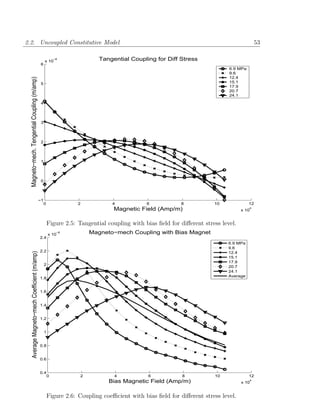
82. 54 Chapter 2. Constitutive relationship of Magnetostrictive Materials
bias magnet is optimum for increased value of average coupling coefficient. These average
values for different stress level is again averaged over the stress level and shown that the
strength of 20-kA/m bias magnet is optimum for efficiency of magnetostrictive actuator
in varied stress level. Average magnetomechanical coefficient with zero magnetic bias is
14.67e-9 (m/amp) (shown in Figure-2.6). This value is generally considered in uncoupled,
linear, bias-less magnetostrictive actuator. From Figure-2.1, it is clear that the linear
model is an approximation from the real behavior of the actuator.
2.2.2 Polynomial Approach
In the polynomial approach [192], every magnetostriction-magnetic field intensity curve
is represented by a fourth order polynomial curve given by.
λ = α0 + α1 H + α2 H 2 + α3 H 3 + α4 H 4 (2.3)
Where, λ represent the magnetostriction and, H is the applied magnetic field. The
constants α0 − α4 are evaluated for each stress level using the data supplied by Etrema
manual, and their values are listed in Table-2.1. A linear interpolation of functional
form for these constants α1 − α4 is estimated as a function of σ, which is used whenever
integration with σ is required in this analysis. This is given by
αi = αi1 σ < σ1 (2.4)
αi(j+1) − αij
αij (σ) = αij + (σ − σj ) σj < σ < σj+1
σj+1 − σj
i = 0, 1, 2, 3, 4 j = 1, 2, 3, 4, ...6
The values of αij ’s and σj ’s are given in Table-2.1. The magnetomechanical constant
Table 2.1: Constants α0 through α4 for different prestress levels [192].
σj , M P a 6.9 9.6 12.4 17.9 24.1 38.0
α0j -50.2987 -81.3171 -58.7017 -2.1391 22.0131 -0.4968
α1j 3.7301 3.2017 1.9530 -0.0931 -0.5268 0.2066
α2j -4.7e-3 -2.3e-3 9.72e-4 5.1e-3 3.6e-3 -3.7006e-4
α3j 2.8406e-6 4.0316e-7 -2.4375e-6 -5.2425e-6 -2.5378e-6 1.3335e-6
α4j -6.4174e-10 1.1572e-10 9.095e-10 1.5458e-9 4.9722e-10 -5.7574e-10
now can be expressed by differentiating Equation-(2.3). This is given by
d = α1 + 2α2 H + 3α3 H 2 + 4α4 H 3 (2.5)

83. 2.2. Uncoupled Constitutive Model 55
2.2.3 ANN Model
As mentioned earlier, magnetostriction varies with of applied magnetic field and stress
level. In this study, the magnetostriction is modelled using a three layer artificial neural
network (ANN) trained by back propagation algorithm for compressive stress level. In
input layer, two input nodes are used; one for applied magnetic field and other for stress
level and in output layer, one output node for magnetostriction is used. This artificial
neural network is trained using the experimental data given in Etrema manual [52] for
different compressive stress level. Due to non-availability of experimental data in tensile
stress level, magnetostriction for tensile stress level is not modelled here. As magnetostric-
tion depends upon stress level and applied magnetic field, using trained neural network,
the corresponding magnetostriction (d33 H3 ) is calculated for applied magnetic field and
stress level.
2.2.3.1 Network Architecture
The network parameters are determined, as is common practice, through trial and error.
This includes the number of layers, the number of nodes in hidden layers and the learning
rates. Number of hidden layers is assumed as one to simplify the study and reduce the
size of network architecture. Hence, the network used consisted of three layers: one input
layer of two neurons (one for each input variable, stress and magnetic field), one hidden
layer of different no of neurons (nodes) and one output layer of one neuron, which in the
present case represents magnetostriction. A study for the performance of network is done
to determine the effect of number of nodes in the hidden layer. Similarly, the effect of
learning rate and learning algorithm is also studied.
2.2.3.2 Study on Number of Nodes in Hidden Layer
Although the increasing number of hidden layer nodes will represent the actuation non-
linearity more accurately, the floating point operation and storage requirement for the
evaluation of magnetostriction for different stress levels and applied magnetic fields using
the trained architecture will also increase. Hence, there will be a tradeoff between the
number of nodes in hidden layer and performance of trained network from the training
and validation samples. Performance of the network can be assessed if one can measure
the error associated with the learning performance and the strains for different number
of nodes in the hidden layer. These are plotted in Figure-2.7 and Figure-2.8. From the

84. 56 Chapter 2. Constitutive relationship of Magnetostrictive Materials
Learning Performance on Hidden Node Number
0.04
1
2
3
4
0.035 5
6
7
0.03
Error(%)
0.025
0.02
0 2 4 6 8 10
Epoch x 10
4
Figure 2.7: Study on the effect of number of node in hidden layer.
x 10
−7 Validation Error
14
12
10
Strain
8
6
4
2
1 2 3 4 5 6 7
No of Node in hidden Layer
Figure 2.8: Study on the effect of number of node in hidden layer.

85. 2.2. Uncoupled Constitutive Model 57
−4
x 10 Validation Sample Point
14
12
10
Magnetostriction
8
6
4
2
0
−2
0 200 400 600 800 1000 1200 1400
Magnetic Field (Oe)
Figure 2.9: Test data from network and sample data set.
x 10
−4 Validation Sample Point
14
12
10
Magnetostriction
8
6
4
2
0
−2
0.5 1 1.5 2 2.5
Stress(Pa) 7
x 10
Figure 2.10: Test data from network and sample data set.

86. 58 Chapter 2. Constitutive relationship of Magnetostrictive Materials
figure, it is found 4-nodded network is optimum. Except 1 and 2-nodded network, train-
ing performance of other networks are comparatively acceptable. But for 3-nodded and
5-nodded architectures, the validation errors are poor compared to 4-nodded architecture.
Average error of validation samples in 4-nodded architecture is around 0.2 micro-strain.
Hence, 4-nodded architecture is considered for further study. Test data is plotted in two
different projection planes one in stress vs. magnetostriction plane and other in applied
magnetic field vs. magnetostriction plane as shown in Figure-2.9 and Figure-2.10 for com-
paring with the data predicted by the network model. In these plots, some of the data
point for small magnetic field has shown very small negative magnetostriction. This neg-
ative magnetostriction will provide negative actuation, and negative magneto-mechanical
coupling that may not be the desired in the actuator application. Since the value of
magnetostriction is negligible for small magnetic field, this negative magnetostriction can
be assumed as zero for the output of network.
2.2.3.3 Study on Learning Rate
The back-propagation algorithm provides an ”approximation” to the trajectory in weight
space computed by the method of steepest descent. The smaller we make the learning
rate, the smaller will the changes to the synaptic weights, and hence smoother will be
the trajectory in weight space. This improvement, however, is attained at the cost of
a slower rate of learning. If, on the other hand, we make the learning rate too large
in order to speed up the rate of learning, the resulting large changes in the synaptic
weights assume such a form that the network may become unstable (i.e. oscillatory). A
simple method of increasing the rate of learning yet avoiding the danger of instability is
to consider a momentum term with the learning rate parameter. This momentum term
will be the certain percentage of the increment of the previous step added to the present
step. The incorporation of momentum in the back-propagation algorithm represents a
minor modification to the weight update, yet it may have some beneficial effects on the
learning behavior of the algorithm. The momentum term may also have the benefit of
preventing the learning process from terminating in a shallow local minimum on the error
surface.
2.2.3.4 Sequential Training Mode
Learning rate is varied from 0.1 to 0.7 at an interval of 0.1 to study its effect on the learning
performance for a 4-nodded hidden layer network. These are plotted in Figure-2.11 and

87. 2.2. Uncoupled Constitutive Model 59
Figure-2.12. Slow learning performance is observed for low learning rate parameter. In
addition, it affects the validation error of the trained network.
2.2.3.5 Training by Batch Mode
Same network is then trained in batch mode for different learning rate parameter. These
are shown in Figure-2.13 and Figure-2.14. From the Figure, we see that as the learning
rate parameter is increased from 0.1 to 0.7, the training rate of the network also increased.
As in the sequential mode, the validation error is also connected with the learning rate.
2.2.3.6 Momentum Effect
Effect of momentum is also studied in the batch mode training with different momentum
parameter, which means that certain percentage of the previous weight-increment is added
to the present weight-increment. The effect of momentum on the overall training process
is shown in Figure-2.15 and Figure-2.16. In the Figure-2.15, it is shown that at to higher
value of learning rate parameter (0.8), the network is not trained properly and it becomes
oscillatory in initial stage of learning. Figure-2.16 gives the training performance with
different values of momentum from 0.1 to 0.7 with the same (0.8) learning rate parameter.
2.2.3.7 Selected Network
Based on the performance of the 3-layer network, following are the configuration that
is used to obtain the constitutive model. The input layer has two neuron (one for each
input variable), one hidden layer of 4 neurons and one output layer of one neuron, which
corresponds to one output variable, namely the magnetostriction. The network is trained
using sequential mode of training. The finished ANN model is delineated through the
connection weights between the input and hidden layers and between the hidden and
output layers, which are listed in Table 2.2 and Table 2.3 respectively.
Standard logistic function y = 1/(1 + e−1.7159v ) is used in hidden layer as acti-
vation function with linear output layer. Input (stress and magnetic field) and output
(magnetostriction) data are normalized for better performance of network as follows.
(σ − σmean )
σn = (2.6)
(max|σ| − σmean )
(H − Hmean )
Hn = (2.7)
(max|H| − Hmean )

88. 60 Chapter 2. Constitutive relationship of Magnetostrictive Materials
Learning Performance For Diff. Learning Rate
0.06
0.1
0.2
0.055 0.3
0.4
0.05 0.5
0.6
0.7
0.045
Error(%)
0.04
0.035
0.03
0.025
0.02
0 2 4 6 8 10
Epoch x 10
4
Figure 2.11: Effect of learning rate on training performance
x 10
−7 Validation Error With Momentum
4.2
4
3.8
3.6
Strain
3.4
3.2
3
2.8
2.6
0.1 0.2 0.3 0.4 0.5 0.6 0.7 0.8
Learning Rate
Figure 2.12: Effect of learning rate on validation performance

89. 2.2. Uncoupled Constitutive Model 61
Learning Performance For Different Learning Rate
0.06
0.1
0.2
0.055
0.3
0.4
0.05 0.5
0.6
0.045 0.7
Error(%)
0.04
0.035
0.03
0.025
0.02
0.015
0 2 4 6 8 10
Epoch x 10
4
Figure 2.13: Effect of learning rate on batch mode training performance.
−7
x 10 Validation Error for Diff. Learning Rate
4.2
4
3.8
3.6
Strain
3.4
3.2
3
2.8
0.1 0.2 0.3 0.4 0.5 0.6 0.7 0.8
Learning Rate
Figure 2.14: Effect of learning rate on validation performance for batch mode learning.

90. 62 Chapter 2. Constitutive relationship of Magnetostrictive Materials
Learning Performance For Different Learning Rate
0.2
0.7
0.18 0.8
0.9
0.16 1.0
0.14
0.12
Error(%)
0.1
0.08
0.06
0.04
0.02
0
0 2 4 6 8 10
Epoch x 10
4
Figure 2.15: Effect of momentum on training performance.
Learning Performance For Different Momentum
0.036
0.1
0.034 0.2
0.3
0.4
0.032 0.5
0.6
0.03 0.7
0.028
Error(%)
0.026
0.024
0.022
0.02
0.018
0 2 4 6 8 10
Epoch x 10
4
Figure 2.16: Effect of momentum on training performance.

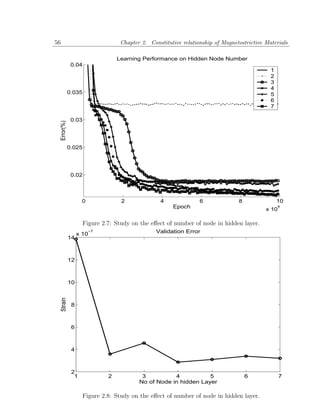
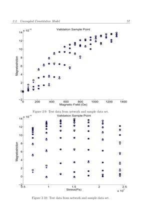
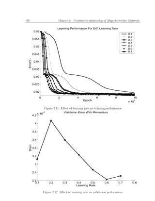
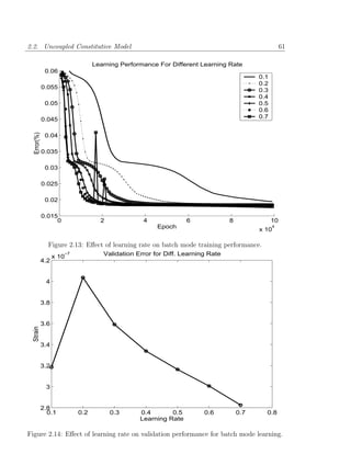
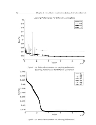
91. 2.2. Uncoupled Constitutive Model 63
(λ − λmean )
λn = (2.8)
(max|λ| − λmean )
In Equation-(2.6), σn is the normalized stress and σmean is mean stress of training samples.
The value of σmean and (max|σ| − σmean ) are 1.5243X107 and 8.857X106 Pa respectively.
Similarly Hn is normalized magnetic field, Hmean is mean magnetic field of training sam-
ples. The value of Hmean and (max|H| − Hmean ) in Equation-(2.7) are both 652 Oe.
Normalized magnetostriction λn is the output of network, from which magnetostriction
is calculated using Equation-(2.8). Where the value of λmean and (max|λ| − λmean ) are
both 0.798X10−3 .
Table 2.2: Connection between input layer and hidden layer.
Hidden Layer Nodes 1 2 3 4
σn -.11946E+01 -.33016E+00 .14013E+01 .14978E+01
Hn .29959E+01 -.28768E+00 -.15922E+01 .19209E+00
Input Bias .128112E+01 -.680953E+00 -.916353E-02 .187534E+01
Table 2.3: Connection between hidden layer and output layer.
Hidden Layer Nodes 1 2 3 4 output bias
λn 1.1240 -.65999 -.63945 1.0767 -1.27577
Figure-2.17 and Figure-2.18 gives the magnetostriction and magneto-mechanical
coupling coefficient for different stress level (from 6.9MPa to 24.1 MPa) according to the
present neural network model. As the network is trained taking data from all the stress
level given in the manual [52], and the network is not validated for different stress level
not given in the manual, there is a possibility of over training of network in other stress
level. Networks become over trained while modelling noises in the responses, which are
not desirable. However, by looking at the output of network for twenty intermediate stress
level shown in these figures, it can be concluded that the network is not over trained.
2.2.4 Comparative Study with Polynomial Representation
Earlier study to model nonlinear actuation of magnetostrictive material was done
considering a fourth order polynomial of magnetic field for each stress level [192]. The
fourth order polynomial representation of magnetostriction required five real parameters
for each curve represented in each stress level. To compute the magnetostriction from a

92. 64 Chapter 2. Constitutive relationship of Magnetostrictive Materials
−3
x 10 Magnetostriction of Comp. Terfenol−D
1.4
1.2
1 6.9 MPa
0.8
Strain
0.6 24.1 MPa
0.4
0.2
0
0 2 4 6 8 10
Magnetic Field(Amp/m) x 10
4
Figure 2.17: Magnetostriction for different stress level.
−8
x 10 Magneto−Mechanical Coefficient
3
6.9 MPa
2.5
2
d(m/Amp)
1.5
1
0.5
24.1 MPa
0
0 2 4 6 8 10
Magnetic Field (Amp/m) 4
x 10
Figure 2.18: Coupling coefficient for different stress level.

93. 2.3. Coupled Constitutive Model 65
specified curve, four floating-point multiplications and four floating-point additions are
required. In addition, polynomial representation required interpolation of magnetostric-
tion for the stress level that has no curve. This requires searching of upper and lower
stress level for those where the polynomial representation is available and using these,
magnetostriction can be computed using appropriate interpolation.
In this work, we use ANN to compute the magnetostriction, especially for nonlinear
magnetostrictive model. The number of floating point operation required for a N nodded
hidden layer network can be assessed as follows. The three layer network considered
is represented by 3N number of weight parameters, N + 1 number of bias parameters
and six numbers of normalization parameters. The input layer has two input node and
output layer has one. Both input and the output is normalized. Total number of floating
point operations required for N -nodded network is N number of division, N number of
exponential computation, 4N +3 number of multiplication and 4N +3 number of addition.
For four-nodded hidden layer network, 23 real parameters are required.
Some of the advantages of ANN over polynomial representation are as follows. In
polynomial representation, if the number of curves are more, searching and storage require-
ment are also more compared to the artificial network model, although the requirement of
floating point operations is less in polynomial representation. Another advantage in using
artificial neural network over polynomial representation is that it has a direct representa-
tion of magnetostriction for a given applied magnetic field and stress level. As opposed
to this, validation of the polynomial representation is not studied with different set of
sample data apart from interpolated data. Magnetostriction according to artificial neural
network (ANN), polynomial approach and experimental data is shown in Figure-2.19 for
stress levels of 6.9, 15.1 and 24.1 MPa. For these stress levels, we see that there is a good
match from all these approaches. For low stress level, in low and high magnetic fields,
polynomial approach gives 50 and 100 ppm errors with experimental results, respectively.
For all stress levels ANN approach gives with in 10 ppm errors in magnetostriction from
experimental results.
2.3 Coupled Constitutive Model
As mention earlier, analysis of smart structures using magnetostrictive materials as either
sensors or actuators has traditionally been performed using uncoupled models. Uncoupled
models make the assumption that the magnetic field within the magnetostrictive material
is constant and proportional to the electric coil current times the number of coil turn per

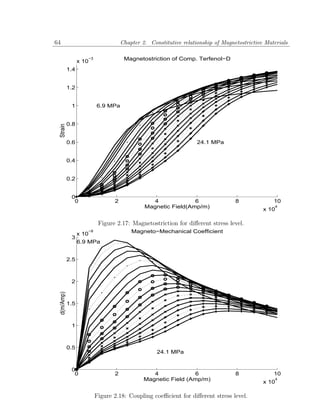
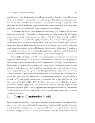
94. 66 Chapter 2. Constitutive relationship of Magnetostrictive Materials
x 10
−3 Compare of Diff. Approach.
1.4
Polynomial
ANN
Experimental
1.2
1
Magnetostriction
0.8 6.9 MPa 15.1 MPa
0.6 24.1 MPa
0.4
0.2
0
0 2 4 6 8 10 12
Magnetic Field (Amp/m) x 10
4
Figure 2.19: Magnetostriction for different stress level.
unit length. Hence actuation and sensing problems are solved by two uncoupled equations,
which are given by the last part of Equation-(2.1) and Equation-(2.2), respectively. This
makes the analysis relatively simple; however this method has its limitations. It is quite
well known that [S], [d] and [µ] all depend on stress level and magnetic field. In the pres-
ence of mechanical loads, the stress changes and so is the magnetic field. Estimating the
constitutive properties using uncoupled model in such cases will give inaccurate predic-
tions. Hence, the constitutive model should be represented by a pair of coupled equations
given by Equations-(2.1) & (2.2) to predict the mechanical and magnetic response. It
is therefore necessary to simultaneously solve for both the magnetic response as well as
the mechanical response regardless of whether the magnetostrictive material is being used
as a sensor or actuator. Due to in-built non-linearity, the uncoupled model may not be

95. 2.3. Coupled Constitutive Model 67
capable of handling certain applications such as (1) modelling passive damping circuits
in vibration control and (2) development of self-sensing actuators in structural health
monitoring. In these applications, the coupled equations require to be solved simultane-
ously. The solution of coupled equations simultaneously is a necessity for general-purpose
analysis of adaptive structures built in with magnetostrictive materials. In general, the
errors that result from using uncoupled models, as opposed to coupled ones, are problem
dependent. There are some cases where very large differences exist in situations, where
an uncoupled model is used over a coupled model [132].
In this work, the coupled case is analyzed with both linear and non-linear model. In
linear-coupled model, magneto-mechanical coefficient, elasticity matrix and permeability
matrix are assumed as constant. In nonlinear-coupled model, mechanical and magnetic
nonlinearity are decoupled in their respective domains. The nonlinear stress-strain re-
lationship is generally represented by modulus of elasticity and the nonlinear magnetic
flux-magnetic field relationship represented by permeability of the material. Magneto-
mechanical coupling coefficient will be assumed as constant in this case.
2.3.1 Linear Model
From Equation-(2.1) and Equation-(2.2), the 3D constitutive model for the magnetostric-
tive material can be written as
{σ} = [Q]{ } − [e]T {H} (2.9)
{B} = [e]{ } + [µ ]{H} (2.10)
Where [Q] is Elasticity matrix, which is the inverse of compliance matrix [S], [µ ] is the
permeability at constant strain. [µ ] and [e] are related to [Q] through
[e] = [d][Q] (2.11)
[µ ] = [µσ ] − [d][Q][d]T (2.12)
For ordinary magnetic materials, where magnetostrictive coupling coefficients are zero,
[µ ]=[µσ ], the permeability.
Consider a magnetostrictive rod element of length L, area A, with Young modulus
Q. If a tensile force F, is applied the rod develops a strain , and hence a stress σ. Total

96. 68 Chapter 2. Constitutive relationship of Magnetostrictive Materials
strain energy in the rod will be
1 1
Ve = σdv = {Q − eH}dv
2 2
1 1
= Q dv − eHdv
2 2
1 1
= ALQ 2 − ALe H (2.13)
2 2
Magnetic potential energy in a magnetostrictive rod is
1 1
Vm = BHdv = {e + µ H}Hdv
2 2
1 1
= eHdv + Hµ Hdv
2 2
1 1
= ALHe + ALµ H 2 (2.14)
2 2
Magnetic external work done for N number of coil turn with coil current I is
Wm = IN µσ HA (2.15)
Mechanical External work done is
We = F L (2.16)
Total potential energy of the system becomes
1 1
Tp = − ALQ 2 + ALe H
2 2
1 1
+ ALHe + ALµ H 2 − IN µσ HA + F L (2.17)
2 2
t2
Using Hamilton’s Principle, δ( t1
Tp dt) = 0, two equations in terms of H and , will
come.
−ALQ + ALeH + F L = 0 (2.18)
ALe + ALHµ − IN µσ A = 0 (2.19)
Dividing both equations by AL, equations will be
F
−Q + eH = − (2.20)
A

97. 2.3. Coupled Constitutive Model 69
IN µσ
e + Hµ = (2.21)
L
As right hand side of Equation-(2.21) is not function of and left hand side is magnetic
flux density (Equation-(2.10)), it can be concluded that the magnetic flux density in this
model is not function of . Hence, it is preserving the flux line continuity. Eliminating H
from Equation-(2.20) and substituting this in Equation-(2.21), stress - strain relationship
of the magnetostrictive material can be written as follows.
H = (Q − F/A)/e (2.22)
IN µσ Ae + Lµ F IN µσ eA + F µ L
= = (2.23)
ALe2 + ALµ Q ALµσ Q
From Equation-(2.23), total strain for applied coil current I and tensile stress F/A can
be written as
=λ+ σ (2.24)
where λ is the strain due to coil current, which is called the magnetostriction, and σ is
the strain due to tensile stress (elastic strain). These are given by
IN µσ Ae
λ= = IN d/L (2.25)
ALµσ Q
Lµ F F
σ = σQ
= (2.26)
ALµ AQ∗
Let Q∗ be the modified elastic modulus and substituting the value of e and µ from
Equation-(2.11) and Equation-(2.12), Q∗ will be
Qµσ Qµσ e2
Q∗ = = σ =Q+ (2.27)
µ µ − d2 Q µ
If the value of µσ is much greater than d2 Q, µ can be assumed equal to µσ and Q∗ can
be assumed as equal to Q. Hence, the total strain of the rod will be same as for the
uncoupled model. The first term in the strain expression is the strain due to magnetic
field, and the second term is the strain due to the applied mechanical loading. However,
for Terfenol-D [52], the value of d2 Q is comparable with µσ . Substituting the value of
strain from Equation-(2.23) in the Equation-(2.22), the value of magnetic field will be
F µ IN
H=− (1 − σ ) + (2.28)
Ae µ L

98. 70 Chapter 2. Constitutive relationship of Magnetostrictive Materials
Note that although the magnetostriction value (IN d/L) in Equation-(2.25) is same for
coupled and uncoupled case, the value of magnetic field is different. Assuming r as the
ratio of two permeabilities or two elastic module, from Equation-(2.27), r can be written
as.
µσ Q∗
r= = (2.29)
µ Q
If the value of r is one, result of coupled analysis is similar with uncoupled analysis.
In Figure-2.20, the value of r is shown in contour plot for different values of constant
strain permeability and modulus of elasticity considering coupling coefficient as 15X10−9
m/Amp. In the Figure-2.20(a), value of r is shown for different values of permeability
and elastic modulus. In the Figure-2.20(b), value of r is shown for different values of
permeability and modified elasticity. In these plots it is clear that for a particular value
of elasticity, if the value of permeability increases, the value of r will decrease. However,
for a particular value of permeability, if the value of elasticity increases the value of r
will increase. In Figure-2.21, the value of r is shown in contour plot for different value
of permeabilities and coupling coefficient considering module of elasticity as 15GPa. In
Figure-2.21(a), value of r is given for different values of constant strain permeability and
coupling coefficient. In Figure-2.21(b), value of r is shown for different values of constant
stress permeability and coupling coefficients. In these plots it is clear that for a particular
value of permeability, if the value of coupling coefficient increases the value of r will
increase. But for a particular value of coupling coefficient if the value of permeability
increases, the value of r will decrease. In Figure-2.22, the value of r is shown in contour
plot for different value of elasticities and coupling coefficient considering constant strain
permeability as 7X10−6 henry/m. In Figure-2.22(a), value of r is given for different values
of modulus of elasticities and coupling coefficient. In Figure-2.22(b), value of r is shown
for different values of modified elasticities and coupling coefficients. In these plots it is
clear that for a particular value of elasticity, if the value of coupling coefficient increases
the value of r will increase. Similarly, for a particular value of coupling coefficient if the
value of elasticity increases, the value of r will increase.
From experimental data given in Etrema manual [52], the best value of Q, µσ and d
is calculated, which will minimize the difference between experimental data and the data
according to Equation-(2.23) by least square approach. In the first set of experimental
data, only magnetostriction value is reported, which is expressed in Equation-(2.25). The

99. 2.3. Coupled Constitutive Model 71
x 10
−6 Ratio of two permeabilities (r)
13
−9
d=15X10 m/Amp
12
1.4
1.2 1.6
11
Permeability (µ )(H/m)
1.8
10
ε
9 1.4 1.6
2
1.8
8
7 2 2.2
1.6
1.4 1.8
6
2.6
2 2.2 2.4
5
1 1.5 2 2.5 3 3.5 4
Modulus of Elasticity (Q)(Pa) x 10
10
(a)
x 10
−6 Ratio of two permeabilities (r)
13
d=15X10−9m/Amp
1.4
1.2
12
1.6
11
1.8
Permeability (µ )(H/m)
10
ε
1.4
9
1.6
1.8
8
2
7
6
2.2
1.6
2.6
2.4
1.8
2
5
0 2 4 6 8 10 12
Modified Elasticity (Q*)(Pa) x 10
10
(b)
Figure 2.20: Ratio of two permeabilities (r) with different values of permeability vs.
modulus of elasticity (a) and modified elasticity (b), considering d=15X10−9 m/Amp .

100. 72 Chapter 2. Constitutive relationship of Magnetostrictive Materials
x 10
−6 Ratio of two permeabilities (r)
13
Q=15 GPa
1.2
1.4
12
Constant Strain Permeability ( µ )(H/m)
1.6
11
1.8
ε
10
1.4
1.2
9
1.6
8
8
2
1.
2
2.
7
1.4
1.2
6
6
2.4
1.
2
8
2.6
1.
2
2.
5
0.8 1 1.2 1.4 1.6 1.8 2 2.2 2.4 2.6
Coupling Coefficient(d)(m/Amp) x 10
−8
(a)
x 10
−5 Ratio of two permeabilities (r)
2.2
Q=15 GPa
8
1.
2
Constant Stress Permeability ( µ )(H/m)
1.6
1.8
σ
2
2
2.
1.6
8
1.
6 2.4
1.4
1.4
6
2.
1.
1.2
2. 2
1.2
2
8
1
1.
4
1.
6
1.
0.8
2
1.
0.6
0.8 1 1.2 1.4 1.6 1.8 2 2.2 2.4 2.6
Coupling Coefficient(d)(m/Amp) x 10
−8
(b)
Figure 2.21: Ratio of two permeabilities (r) with different values of coupling coefficient
vs. constant strain permeability (a) and constant stress permeability (b), considering
Q=15GPa.

101. 2.3. Coupled Constitutive Model 73
x 10
10 Ratio of two permeabilities (r)
4
2
3.5
3
2.5
1.5
4
3.5
Modulus of Elasticity (Q)(Pa)
3
3.
3
5
2.
2
5
1.5
2.5
2 2.5
2
1.
5
1.5
ε −6
µ =7X10 H/m 2
1
0.8 1 1.2 1.4 1.6 1.8 2 2.2 2.4 2.6
Coupling Coefficient(d)(m/Amp) x 10
−8
(a)
x 10
10 Ratio of two permeabilities (r)
18
16 µε=7X10−6H/m
4
14
Modified Elasticity (Q )(Pa)
12
*
3 3.5
10
8
2 2.5
3
6
1.5
2.5
4 2
1.5 2
2
0
0.8 1 1.2 1.4 1.6 1.8 2 2.2 2.4 2.6
Coupling Coefficient(d)(m/Amp) x 10
−8
(b)
Figure 2.22: Ratio of two permeabilities (r) with different values of coupling coefficient vs.
modulus of elasticity (a) and modified elasticity (b), considering µ = 7X10−6 henry/m.

102. 74 Chapter 2. Constitutive relationship of Magnetostrictive Materials
value of coupling coefficient is calculated minimizing the total square error, λError .
λError = (λexp − λ)2 (2.30)
Similarly in the second set of experimental data, strain due to compressive stress ( σ ) is
reported. The expression for the value of elastic strain, σ is given in Equation-(2.26). In
this expression, the value of Q∗ is calculated minimizing the total square error Error
σ .
Error exp 2
σ = ( σ − σ) (2.31)
From Equation-(2.30), using first set of experimental data (plotted in Figure-2.1), the
value of d is calculated as 14.8X10−9 (m/amp). From Equation-(2.31), using the second
set of experimental data (plotted in Figure-2.3), the value of Q∗ is 33.4 GPa. Assuming
constant strain permeability (µ ) of the material is 7X10−6 henry/m, the value of r is
1.6, constant stress permeability (µσ ) is 11.2X10−6 henry/m and Q is 20.8 GPa. From
these studies it is clear that for giant magnetostrictive material, like Terfenol-D, coupled
analysis will give better result than uncoupled analysis. But for magnetostrictive material
with low coupling coefficient, the uncoupled analysis will give similar result with coupled
analysis.
The coupled linear model cannot model the high nonlinearity of magnetostriction λ,
which is required for design of actuator. Even considering nonlinear magnetic (magnetic
field-magnetic flux) and mechanical (stress-strain) relationships with linear coupling coef-
ficient, nonlinear relationships of magnetostriction cannot be modelled as it is a function
of coil current, coil turn per unit length of actuator and magneto-mechanical coefficient
(Equation-(2.25)). In the next section, we introduce a nonlinear model with a constant
coupling coefficient, which can model the non-linear constitutive model exactly for con-
stant magnetic coupling.
2.3.2 Nonlinear Coupled Model
The model developed in this section is based on a coupled magneto-mechanical formula-
tion, which allows accurate prediction of both the mechanical and the magnetic response
of a magnetostrictive device with nonlinear magnetic and mechanical properties. Non-
linearity in this model is introduced using two nonlinear curves, one for stress-strain rela-
tion and the second for magnetic field-magnetic flux relation, which enables to decouple
the non-linearity in mechanical and magnetic domains. Magneto-mechanical coefficient is
considered as a real parameter scalar value. Two-way coupled magneto-mechanical theory

103. 2.3. Coupled Constitutive Model 75
is used to model magnetostrictive material. The formulation starts with the constitutive
relations. In earlier coupled-linear model, stress (σ) and magnetic flux density (B) was
expressed as a function of the components of strain ( ) and magnetic field (H) as per
Equation-(2.9) and Equation-(2.10). Main draw back with such an approach is that the
non-linearity between magnetic domain (µ ) and mechanical domain (Q) are not uncou-
pled. Hence, it is difficult to model non-linearity in earlier representation. To address
these issues, a different approach is used in which Equation-(2.9) and Equation-(2.10) are
rearranged in terms of the mechanical strain ( ) and the magnetic flux density (B). In
doing so, the mechanical non-linearity is limited to stress-strain relationship and magnetic
non-linearity is limited to magnetic field-magnetic flux relationship.
One-dimensional nonlinear modelling is again studied using one-dimensional exper-
imental data from Etrema manual. The constitutive equation can now be rewritten in
terms of magnetic flux density (B) and strain ( ), as
σ = E − fT B (2.32)
H = −f + gB (2.33)
Where
g = (µ )−1
f = gdQ = e/µ (2.34)
E = Q + Qdf = Q∗
Like linear case, we will again consider a magnetostrictive rod element of length L, area
A, applied tensile force F , strain , stress σ, elastic modulus E. Total strain energy in
the rod will be
1 1
Ve = AL σ = (E − f B)
2 2
1 1
= ALE 2 − AL f B (2.35)
2 2
Magnetic potential energy in magnetostrictive rod is given by
1 1
Vm = ALBH = AL(−f + gB)B
2 2
1 1
= − ALBf + ALgB 2 (2.36)
2 2

104. 76 Chapter 2. Constitutive relationship of Magnetostrictive Materials
Magnetic external work done for N turn coil with coil current I is
Wm = IN BA (2.37)
Mechanical External work done is
We = F L (2.38)
Total potential energy of the system is equal to T p = −V e − V m + W m + W e.
1 2 1
Tp = − ALE + AL f B − ALgB 2 + IN BA + F L (2.39)
2 2
Using Hamilton’s Principle, two equations of B and will be
−ALE + ALf B + F L = 0 (2.40)
AL f − ALgB + IN A = 0 (2.41)
Dividing by the Volume, AL, Equation-(2.40) and Equation-(2.41) will become
F
E − fB = (2.42)
A
IN
−f + gB = (2.43)
L
Eliminating B from Equation-(2.42) and substituting this in Equation-(2.43), stress-strain
relationship for the magnetostrictive material can be obtained as
E − F/A
B= (2.44)
f
F/A + IN f /(gL)
= (2.45)
E − f 2 /g
Assuming E ∗ as the magnetically free elastic modulus
E ∗ = E − f 2 /g = Q (2.46)
Total strain for applied coil current I and tensile force, F will be
IN f F
= ∗)
+ (2.47)
(gLE AE ∗

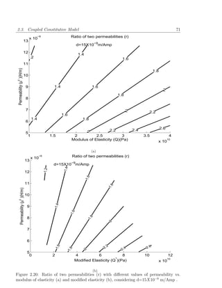
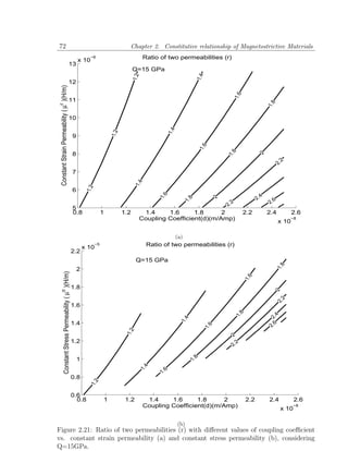
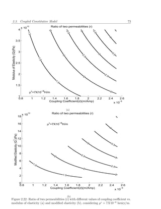
105. 2.3. Coupled Constitutive Model 77
Here E = Q ∗ is the elastic modulus for a magnetically stiffened rod and Q = E ∗ is for
magnetically flexible rod. Magnetically stiffened means that the magnetic flux B=0 inside
the rod as rod is wound by short circuited coils. Magnetically flexible means the rod is
free from any coil. E-Q relation can be obtained form Equation-(2.34).
To model the one-dimensional nonlinear magnetostrictive stress-strain and magnetic
field-magnetic flux relationships, Equation-(2.32) and Equation-(2.33) can be written as,
E( ) − f B = σ (2.48)
IN
−f + g(B) = (2.49)
L
where f is the real parameter of scalar value, and - E( ), B - g(B) are two real parameter
nonlinear curves. The basic advantage of this model is that only two nonlinear curves
are required for representing nonlinearity reported in different stress levels. As opposed
to this approach, in straight forward polynomial representation of magnetostriction [192],
one requires single nonlinear curve for every stress level. To get the coefficients of two
nonlinear curves and the value of real parameter f , experimental data from Etrema manual
[52] is used. From strain, applied coil current and stress level available in the manual, these
coefficients are evaluated. Considering modulus elasticity as 30GPa, and f as 75.3X106
m/Amp as an initial guess, the values of magnetic flux density, B are calculated from
Equation-(2.48). Similarly from Equation-(2.49), values of g(B) are evaluated. From
these B and g(B) values, curves of B − g(B) is computed. This curve is used to get
mechanical relationship. Here, the value of B is computed from B − g(B) relationship.
From this value of B, using Equation-(2.48), values of E( ) is calculated. From the
E( ) and values, the mechanical nonlinear curve of − E( ) relationship is computed. In
summary, first the magnetic nonlinear curve is evaluated from mechanical nonlinear curve
and mechanical nonlinear curve is evaluated from magnetic nonlinear curve with the help
of experimental data given in Etrema manual [52]. This iteration will continue till both
mechanical curve and magnetic curve converges. Thus, with the help of experimental
data given in Etrema manual [52] and Equations-(2.48) and (2.49), nonlinear mechanical
and magnetic relationship is evaluated. Initial values of modulus of elasticity and f are
computed on trial and error basis.
For sensor device, where coil current is assumed as zero, strain and the value of
magnetic flux due to the application of stress is given by
g(B)
= (2.50)
f

106. 78 Chapter 2. Constitutive relationship of Magnetostrictive Materials
E( ) − σ
B= (2.51)
f
Nonlinear curves for magnetic and mechanical properties are shown in Figure-2.23. These
two nonlinear curves are represented as sixth order polynomial given in Equation-(2.52)
and Equation-(2.53). Coefficients of these polynomials curves are given in Table-2.4,
where unit of B is tesla, g(B) is Amp/m and E( ) is Pa. The value of magneto-mechanical
coupling parameter (f ) is 75.3X106 m/amp, which is reciprocal of 13.3X10−9 amp/m.
Table 2.4: Coefficients for sixth order polynomial.
c d a b
6 0 0 4.5419e+28 1.5853e-50
5 -2.1687e+06 -1.9526e-27 7.6602e+25 -6.1288e-44
4 1.5211e+06 1.1589e-21 -4.2662e+22 -1.0355e-34
3 3.5828e+05 -2.0047e-16 -6.6788e+19 -4.0508e-27
2 -2.1062e+05 2.0096e-12 2.3911e+16 1.0806e-19
1 2.2754e+05 4.7789e-06 1.2539e+13 2.7977e-11
0 -8.8129e+03 4.4239e-02 3.3893e+10 -1.9704e-05
g(B) = c5 ∗ B 5 + .. + c1 ∗ B + c0
B = d5 ∗ g(B)5 + .. + d1 ∗ g(B) + d0 (2.52)
6
E( ) = a6 ∗ + .. + a1 ∗ + a0
= b6 ∗ E( )6 + .. + b1 ∗ E( ) + b0 (2.53)
On the basis of these two curves given in Equation-(2.52) and Equation-(2.53) and
parameter (f ), strain, magnetostriction vs. applied magnetic field for different stress level
are plotted in Figure-2.24. The experimental data of strain-magnetic field relationships
for different stress level is almost matching with this model. Similarly strain-compressive
force and elastic modulus for different magnetic field level is plotted in Figure-2.25. Elastic
modulus initially decreases and then increases for each magnetic field level, which is also
reported in [52].
Computation of Flux and Strain from Coil Current and Stress: As two nonlinear
curves are related in these relationships, the calculation of magnetic flux and strain from
stress and coil current is an iterative procedure. Initially, the value of magnetic flux, B
is assumed a certain value. From B − g(B) curve, the value of g(B) is evaluated. From

107. 2.3. Coupled Constitutive Model 79
x 10
7 Strain vs. Stress
5
4
3
2
Stress (Eε)(Pa)
1
0
−1
−2
−3
Model
Exp
−4
−1 −0.8 −0.6 −0.4 −0.2 0 0.2 0.4 0.6 0.8 1
Strain (ε) x 10
−3
(a)
Magnetic Field vs. Magnetic Flux Density
0.7
0.6
0.5
Magnetic Flux Density (B) (T)
0.4
0.3
0.2
0.1
0
−0.1
Model
Exp
−0.2
−1 −0.5 0 0.5 1 1.5 2
Magnetic Field g(B) (Amp/m) x 10
5
(b)
Figure 2.23: Nonlinear curves (a) Strain vs. Stress curve (b) Magnetic field vs. Magnetic
flux density curve.

108. 80 Chapter 2. Constitutive relationship of Magnetostrictive Materials
x 10
−3 Field vs. Strain in Different Stress Lavel
1
0.8
0.6
0.4
0.2
Strain (ε)
0
−0.2
−0.4
−0.6
−0.8
Model
Exp
−1
0 2 4 6 8 10 12
Magnetic Field (Amp/m) x 10
4
(a)
x 10
−3 Field vs. λ in Different Stress Lavel
1.5
Magnetostriction (λ)
1
0.5 6 MPa
8 MPa
10MPa
12MPa
14MPa
16MPa
18MPa
20MPa
22MPa
24MPa
0
0 2 4 6 8 10 12
Magnetic Field (Amp/m) x 10
4
(b)
Figure 2.24: Nonlinear curves in different stress level (a) Magnetic field vs. Strain (b)
Magnetic field vs. Magnetostriction.

109. 2.3. Coupled Constitutive Model 81
x 10
7 Stress vs. Strain in Diff. Field Lavel
4
0 Amp/m
5000
10000
3.5 15000
20000
25000
30000
3 35000
Compressive Stress (Pa)
40000
2.5
2
1.5
1
0.5
0
0 0.2 0.4 0.6 0.8 1 1.2 1.4 1.6 1.8
Elastic Compressive Strain (εσ) −3
x 10
(a)
x 10
10 Elastic Strain vs. Modulus in Diff. Field
10
0 Amp/m
5000
9 10000
15000
20000
8 25000
30000
35000
7 40000
Elastic Modulus (Pa)
6
5
4
3
2
1
0
0 0.2 0.4 0.6 0.8 1 1.2 1.4 1.6 1.8
Elastic Strain (εσ) x 10
−3
(b)
Figure 2.25: Nonlinear curves for different field level (a) Stress vs. Strain (b) Modulus
vs. Strain.

110. 82 Chapter 2. Constitutive relationship of Magnetostrictive Materials
Equation-(2.43) the value of strain is evaluated considering magnetic field as coil current
times coil turn per unit length of actuator. Using this strain, from the − E( ) curve the
value of E( ) can be found. From Equation-(2.42), the value of B can be determined.
If this B value is not same as assumed, this iteration will be continued until the value
converges.
2.3.3 ANN Model.
To avoid iterative procedure mentioned in the nonlinear model, one three layer artificial
neural network is developed, which gives direct nonlinear mapping from the magnetic field
and the stress to the magnetic flux density and the strain (Figure-2.26). Standard logistic
function y = 1/(1 + e−1.7159v ) is used in the hidden layer as activation function with linear
output layer. The input (stress and magnetic field) and the output (strain and magnetic
flux density) data are normalized for better performance of network.
(σ − σmean )
σn = (2.54)
(max|σ| − σmean )
(H − Hmean )
Hn = (2.55)
(max|H| − Hmean )
( − mean )
n = (2.56)
(max| | − mean )
(B − Bmean )
Bn = (2.57)
(max|B| − Bmean )
σn , the normalized stress is calculated using Equation-(2.54). The value of σmean and
(max|σ| − σmean ) are −1.57966X107 and 0.830345X108 Pa respectively. Similarly Hn is
normalized magnetic field, is calculated from Equation-(2.55). The value of Hmean and
(max|H|− Hmean ) in Equation-(2.55) are both 750 Oe. Normalized strain n is the output
of network, from which strain is calculated using Equation-(2.56). The value of mean and
(max| |− mean ) are 0.203245X10−03 and 0.106504X10−02 respectively. In Equation-(2.57)
the value of Bmean is 0.385126 tesla and the value of (max|B| − Bmean ) are 0.319818 and
0.499656 tesla respectively. To train this network, some training and validation samples
are generated through iterative process stated earlier. Weight and bias parameter of the
trained network is given in Table-2.5 and Table-2.6, respectively. Different validation
studies are also carried out.

111. 2.3. Coupled Constitutive Model 83
NORMALISED
NORMALISED MAGNETOSTRICTION MAGNETOSTRICTION
STRESS STRESS
NORMALISED
MAGNETIC MAGNETIC
FIELD FIELD
NORMALISED MAGNETIC
MAGNETIC FLUX
FLUX DENSITY
DENSITY
INPUT LAYER HIDDEN lAYER OUTPUT LAYER
Figure 2.26: Artificial neural network architecture
Table 2.5: Connection between input layer and hidden layer.
Input Layer Hidden Hidden Hidden Hidden
Neurons Node 1 Node 2 Node 3 Node 4
Hn 4.6187 -2.1241 -.15066 .38726
σn 1.2866 -1.3195 -.43318 .031765
Input Bias 2.2483 -.25721 -.61579 .088719
2.3.4 Comparison between Different Coupled Models.
Comparative studies of different models are done taking a magnetostrictive rod with vary-
ing magnetic field and stress level. Three different stress levels (6.9 MPa,15.1 MPa and
24.1MPa) are taken to compute the total strain and magnetic flux density in the rod for
varying magnetic field level and shown in Figure-2.27. In Figure-2.27(a), total strain is
shown according to linear, polynomial, ANN and experimental approaches. Both polyno-
mial and ANN approach is showing close result with the experimental data throughout
the magnetic field range. Where as in linear model, results are not matching with the
experimental data throughout the magnetic field range. But, this model can be used in
low magnetic field level for medium stress level and in medium field level for high stress
level. For low stress level, linear model can be used in an average sense. In the absence of
experimental data (Etrema manual) of magnetic flux density, only computational results
are shown in Figure-2.27(b). Magnetic flux density is shown according to linear, polyno-

112. 84 Chapter 2. Constitutive relationship of Magnetostrictive Materials
x 10
−3 Strain in Diff. Approach.
1.5
Linear
Polynomial
ANN
Experimental
1
0.5 6.9 MPa
Strain
15.1 MPa
0
−0.5 24.1 MPa
−1
−1.5
0 2 4 6 8 10 12
Magnetic Field (Amp/m) x 10
4
(a)
Flux in Diff. Approach.
1.2
Linear
Polynomial
ANN
1
0.8
Magnetic Flux Density (T)
0.6
0.4 6.9 MPa
0.2
15.1 MPa
0
24.1 MPa
−0.2
−0.4
0 2 4 6 8 10 12
Magnetic Field (Amp/m) x 10
4
(b)
Figure 2.27: Nonlinear curves for different stress level (a) Strain vs. Magnetic field (b)
Magnetic flux density vs. Magnetic field.

113. 2.4. Summary 85
Table 2.6: Connection between hidden layer and output layer.
Output Layer Neurons n Bn
Hidden Node 1 .63447 .67409
Hidden Node 2 -.53313 -.23172
Hidden Node 3 -.69546 -.071654
Hidden Node 4 .48235 2.1900
Output Bias Node -.29930 -1.5467
mial and ANN approach. Similar to strain result, results of ANN model and polynomial
model are in excellent agreement. However, the results of linear model are not matching
through out the magnetic field range. In the linear model, for medium stress level, the
magnetic flux density is matching with the nonlinear model. For high and low stress level,
linear model can be used in an average sense.
2.4 Summary
This study is mainly intended for anhysteretic linear, nonlinear, uncoupled and coupled
constitutive relationship of magnetostrictive material. Nonlinearity in these relationships
is studied using polynomial representation and artificial neural network (ANN).
In uncoupled model, sensor and actuator equations are separately studied assum-
ing that the magnetic field as strain independent. In linear-uncoupled model, modulus
of elasticity, permeability and magnetomechanical coupling coefficient are considered as
constant. In nonlinear–uncoupled model, magnetostriction is represented through a three
layer artificial neural network for actuation property, which is trained and validated from
Etrema manual.
Coupled model is studied without assuming any direct relationship of magnetic
field. In linear-coupled model, elastic modulus, permeability and magnetoelastic constant
is assumed as constant. But this model cannot predict the highly nonlinear properties
of magnetostrictive material. In nonlinear-coupled model, nonlinearity is decoupled in
magnetic domain and mechanical domain using two nonlinear curves for stress-strain
and magnetic flux density-magnetic field intensity. In this model, the computation of
magnetostriction requires the value of magnetic flux density, which comes through an
iterative process for nonlinearity of curves. To avoid this iterative computation, one three
layer artificial neural network is developed, which will give nonlinear mapping from the
stress level and the magnetic field to the strain and the magnetic flux density. Finally,

114. 86 Chapter 2. Constitutive relationship of Magnetostrictive Materials
comparative study of linear, polynomial and ANN approach is performed and shown
that linear coupled model can predict the constitutive relationships in an averaged sense
only. Nonlinear models are shown to predict experimental results exactly throughout the
magnetic field range.
In the next and the subsequent chapter, we will use these material models in the
finite element model and qualitatively show the differences in the responses predicted by
these models. It will also be shown how these models will have an impact on the SHM
studies.

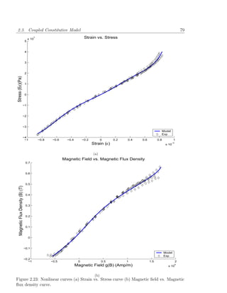
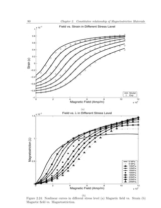
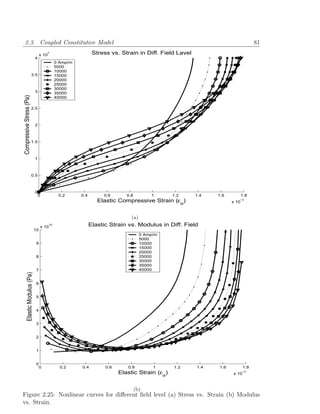
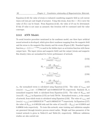
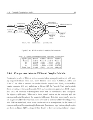
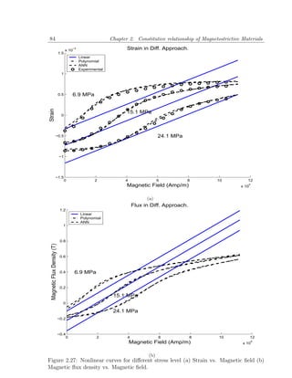
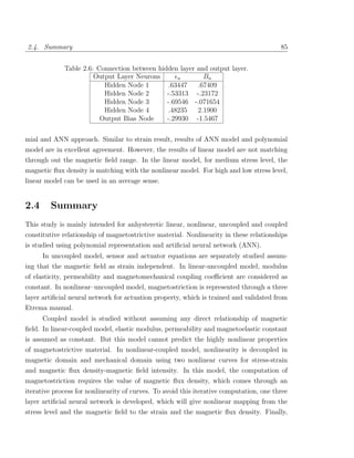
115. Chapter 3
FEM with Magnetostrictive
Actuators and Sensors
3.1 Introduction
In the last chapter, various material models (linear, nonlinear, coupled and uncoupled)
were formulated and the range of its applicability were discussed. In this chapter, these
will be incorporated in the conventional 3-D Finite Element (FE) formulation. From the
3-D FE models, 1-D and 2-D models will be deduced and the effect of different material
models on the healthy and damaged 1-D and 2-D laminated composite structures will be
investigated. In particular, the impact of different material models on the SHM studies
will be highlighted.
3.1.1 Existing Literature
There is a very few literature available on the FE formulation for composite structure
with embedded magnetostrictive patches. Kannan and Dasgupta [174] developed quasi-
static Galerkin finite-element theory for modelling magneto-mechanical interactions at
the macroscopic level considering body forces and coupled constitutive nonlinearities.
Benbouzid et al. modelled the static [35] and dynamic [37] behavior of the nonlinear
magneto-elastic medium for magneto-static case using finite element method. Magneto-
mechanical coupling was incorporated considering both permeability and elastic modulus
as functions of stress and magnetic field. In reference [38], finite elements were used for
modelling different magnetic circuits with leakage flux of a basic actuator configuration.
However, none has provided a convenient way for analysis of magnetostrictive smart
structure considering coupled magneto-mechanical features.
87

116. 88 Chapter 3. FEM with Magnetostrictive Actuators and Sensors
In this chapter, a new finite element formulation for structures with in-built mag-
netostrictive patches that can handle coupled analysis is presented. Here, both magnetic
and mechanical degrees are considered as unknown degrees of freedom. In the present
approach, smart patches are introduced in the laminates to induce actuation strains on
the application of magnetic field. This changes the state of stress in the sensing patch
and hence the magnetic flux density through enclosed magnetic coil changes, resulting in
a voltage across the sensing coil.
Next these elements are used for structural health monitoring applications and
shown that sensitivity of damage in open circuit voltages for SHM is comparable with
the error induced due to uncoupled assumption in the finite element analysis. Finally
this chapter concludes that for the SHM application with magnetostrictive sensor and
actuator, coupled analysis is required for true estimation of the response of the structure.
This chapter is organized as follows. First the variational formulation is given to
obtain the mass, stiffness and coupling stiffness of the system. The main aim of the
study is to bring out the effect of magneto-mechanical coupling on the overall response
of laminated composite structure. For this purpose numerical study is performed on
composite structures containing two patches, one acting as an actuator and the other as
a sensor for varying current amplitude and ply sequence. Both static, frequency response
and time response analysis are performed to bring out the essential difference in responses
between coupled and uncoupled models. The chapter is then concluded with a brief
summary.
3.2 3D Finite Element Formulation
Finite element formulation begins by writing the associated energy in terms of nodal
degrees of freedom by assuming the displacement and magnetic field variation over each
element. That is, the displacement field {U } can be written as
{U } = {u v w}T (3.1)
where u(x, y, z, t), v(x, y, z, t) and w(x, y, z, t) are the displacement component in x, y and
z direction respectively. These displacements are obtained from element nodal displace-
ments {U e (t)}, through the element shape function, [NU (x, y, z)] as
{U } = [NU ]{U e } (3.2)

117. 3.2. 3D Finite Element Formulation 89
The strains { } in terms of displacements {U }, are obtained as
{ }={ xx yy zz γyz γxz γxy }T = [L]{U } (3.3)
Where [L] is given by  
∂
∂x
0 0
 0 ∂
0 
 ∂y 
 0 0 ∂ 
 ∂z 
[L] =  ∂ ∂  (3.4)
 0 ∂z ∂y 
 ∂ ∂ 
 ∂z 0 ∂x

∂ ∂
∂y ∂x
0
Using Equation-(3.2) in Equation-(3.3), the strains can be written as
¯
{ } = [B]{U e } (3.5)
¯
where [B] is strain-displacement matrix and can be expressed as
¯
[B] = [L][NU ]. (3.6)
Similarly Magnetic field vector in the three coordinate directions {H} can be written as
{H} = {Hx Hy Hz }T (3.7)
These magnetic fields are obtained from element nodal magnetic fields {H e }, through the
shape function, [NH (x, y, z)] as
{H} = [NH ]{H e } (3.8)
Strain Energy in magnetostrictive material over a volume v is given by,
1
Ve = { }T {σ}dv
2 v
Substituting for {σ} from Equation-(2.9), { } from Equation-(3.5) and {H} from Equation-
(3.8), this can be written as
1
Ve = { }T {[Q]{ } − [e]T {H}}dv
2 v
1 1
= { }T [Q]{ }dv − { }T [e]T {H}dv
2 v 2 v
1 e T 1
= {U } [KU U ] {U e } − {U e }T [KU H ] {H e } (3.9)
2 2

118. 90 Chapter 3. FEM with Magnetostrictive Actuators and Sensors
where
¯T ¯ ¯ T
[KU U ] = [B] [Q][B]dv, [KU H ] = [B] [e]T [NH ]dv. (3.10)
v v
Where [KU U ] is the stiffness matrix associated with mechanical degrees of freedom and
[KU H ] is the coupling stiffness matrix that couples the mechanical and magnetic degrees
of freedoms. Kinetic Energy in magnetostrictive material is
1 ˙ T
˙
Te = {U } [ρ]{U }dv (3.11)
2 v
˙
where {U } is velocity vector, ρ is density of the material. Substituting {U } from Equation-
(3.2), the kinetic energy can be written as
1 ˙ ˙
Te = {[NU ]{U e }}T [ρ][NU ]{U e }dv
2 v
1 ˙e T ˙ 1 ˙ T ˙
= {U } [NU ]T [ρ][NU ]dv{U e } = {U e } [MU U ] {U e } (3.12)
2 v 2
where the mass matrix for mechanical degrees of freedom can be written as
[MU U ] = [NU ]T [ρ][NU ]dv (3.13)
v
Magnetic Potential Energy in magnetostrictive material is given by
1
Vm = {B}T {H}dv (3.14)
2 v
Substituting {B} from Equation-(2.10), { } from Equation-(3.5) and {H} from Equation-
(3.8), magnetic potential energy can be written as,
1
Vm = {[e]{ } + [µ ]{H}}T {H}dv
2 v
1 e T 1
= {U } [KU H ]{H e } + {H e }T [KHH ]{H e } (3.15)
2 2
where [KHH ] is stiffness matrix of magnetic degrees of freedom, which can be expressed
as
[KHH ] = [NH ]T [µ ]T [NH ]dv. (3.16)
v
Magnetic External Workdone for N turn coil with coil current I, is given by
Wm = IN {[µσ ]{H}} . dA
A
(3.17)

119. 3.2. 3D Finite Element Formulation 91
If n is the coil tern per unit length, A is the cross sectional area of the magnetostrictive
patch and {lc } is the direction cosine vector of coil axis, the above expression can be
written as
Wm = In{lc }T [µσ ]{H}dv
v
= {FH }T {H e } (3.18)
where {FH } is given by
{FH } = In{lc }T [µσ ][NH ]dv (3.19)
v
Mechanical External Workdone is
We = {b}T {U }dv + {τ }T {U }dS
v S
T e
= {R} {U } (3.20)
where {b} is body force vector. and {τ } is surface force vector acting on an area S. {R}T
is equivalent nodal load for external mechanical forces of the magnetostrictive material.
t2
Applying the Hamilton’s Principle ∂( t1
(Te − Ve + Vm + Wm + We )dt) = 0, we can
the governing FE equation. This takes a varied form for uncoupled and coupled model.
These are given below.
3.2.1 Uncoupled Model
In uncoupled model magnetic field, H is considered independent of mechanical condition
[216], and is a function of coil current I, which is given by
H = kc I (3.21)
Where kc is coil constant. Hence, in uncoupled model only mechanical degrees of freedom,
{U e } are unknowns. Substituting this in the Hamiltonian’s Equation, the governing
differential equation becomes
¨
[MU U ]{U e } + [KU U ]{U e } = [KU H ]{H e } − {R} (3.22)
Where He is calculated using Equation-(3.21).

120. 92 Chapter 3. FEM with Magnetostrictive Actuators and Sensors
3.2.2 Coupled Model
Unlike uncoupled model, in the coupled model, the mechanical and magnetic degrees
of freedom are considered as unknown. Hence, Hamiltonian’s principle gives following
Equations.
MU U 0 ¨
Ue KU U −KU H Ue −R
¨ + = (3.23)
0 0 He KHU KHH He FH
Note that the generalized stiffness matrix is not a symmetric matrix. Both the equations,
sensing and actuation are coupled through the off-diagonal, sub-matrix of the stiffness
matrix. Expanding Equation-(3.23), we get
¨
[MU U ]{U e } + [KU U ]{U e } − [KU H ]{H e } = −R (3.24)
and
[KU H ]T {U e } + [KHH ]{H e } = {FH }T
or {H e } = [KHH ]−1 {{FH }T − [KU H ]T {U e }} (3.25)
Substituting {H e } from Equation-(3.25) in Equation-(3.24) we get
¨
[MU U ]{U e } + [KU U ]{U e } = {F } (3.26)
where
[KU U ] = [[KU U ] + [KU H ][KHH ]−1 [KU H ]T ]
{F } = [KU H ][KHH ]−1 {FH } − {R} (3.27)
3.3 Computation of Sensor Open Circuit Voltage
After the computation of nodal displacement and velocities, we can compute the sensor
open circuit voltage. This is particularly of great interest in structural health monitoring
studies. In this section, we derive the necessary expression for both coupled and uncoupled
models.
If the sensor coil current is considered as zero, after determining the mechanical and
magnetic degrees of freedom, sensor open circuit voltage can be post processed in both
uncoupled and coupled model. Using Faraday’s law, open circuit voltage V in the sensing
coil can be calculated from magnetic flux passing through the sensing patch.

121. 3.3. Computation of Sensor Open Circuit Voltage 93
3.3.1 Uncoupled Model
In the uncoupled model, the nodal magnetic field is zero as per Equation-(3.21) with
zero sensor coil current. To get the open circuit voltage, magnetic flux density can be
expressed in terms of strain from the sensing equation, (Equation-(2.10)) as
¯
{B} = [d]{σ} = [d][Q]{ } = [e]{ } = [e][B]{U e } (3.28)
Now using Faraday’s law, open circuit voltage of the sensor can be calculated as
∂
V = −Ns [d]{σ} . dA (3.29)
A ∂t
This can be converted to volume integration as before and the expression for voltage
become
∂ ˙
V = −ns {lc }T [e]{ }dv = {Fv }T {U e } (3.30)
∂t v
where {Fv }T for uncoupled model becomes
{Fv }T = −ns {lc }T ¯
[e][B]dv (3.31)
v
3.3.2 Coupled Model
Magnetic flux density is computed from nodal magnetic field, which is obtained from
finite element analysis. Thus open circuit voltage in the sensor can be calculated from
the expression
∂ σ
V = −Ns − {µ H} . dA (3.32)
A ∂t
where Ns is the total coil turn of the sensing patch. Dividing by the length of the patch
and pre-multiplying with the direction cosine vector of coil axis, the above area integration
with dot product is converted to volume integration. Substituting {H} from Equation-
(3.8), the open circuit voltage can be written as
∂ σ
V = ns {lc }T {µ H}dv
v ∂t
∂
= ns {lc }T {µσ H}dv (3.33)
∂t v

122. 94 Chapter 3. FEM with Magnetostrictive Actuators and Sensors
Substituting {He } from Equation-(3.25) in the above equation it can be written as
∂
V = −ns {lc }T {µσ [NH ]}dv [KHH ]−1 [KU H ]T {U e }
v ∂t
˙
= {Fv } {U e }
T
(3.34)
where {Fv }T is
{Fv }T = −ns {lc }T {µσ [NH ]}dv [KHH ]−1 [KU H ]T . (3.35)
v
3.4 Numerical Experiments
The goal of the analysis is to bring out the effect of coupling on the overall response of 1-D
and 2-D composite structures. Hence, for most of the analysis, the results are compared
with the uncoupled model to see the effect of coupling. Here we consider four examples
of one and two dimensional structures. The first is 1-D magnetostrictive rod model, the
second is a composite beam model based on first order shear deformation theory. The
third and fourth examples considered plate elements and 2D plane stress/strain elements,
respectively. Figure-3.1 shows the various finite elements, with nodes and degrees of
freedom. For these examples, static, frequency response and time history analysis are
performed to bring out the importance of coupled analysis in the context of structural
health monitoring.
3.4.1 Axial Deformation in a Magnetostrictive Rod
To demonstrate the effect of coupling, the above 3-D Equations-(3.24,3.25) reduced to
simple 1-D model with mechanical displacement field (u, v, w) as
u(x, y, z, t) = u(x); v = 0; w=0 (3.36)
and magnetic field H can be reduced as
Hx (x, y, z, t) = H(x); Hy (x, y, z, t) = 0; Hz (x, y, z, t) = 0. (3.37)
Here, a magnetostrictive rod of length L, cross sectional area A, modulus of Elasticity E,
magneto-mechanical strain coefficient d and constant stress permeability µσ is considered.
For finite element formulation, we use the conventional interpolation function that is,

123. 3.4. Numerical Experiments 95
Figure 3.1: Various elements with node and degrees of freedom.

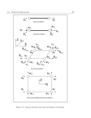
124. 96 Chapter 3. FEM with Magnetostrictive Actuators and Sensors
u(x) = a0 + a1 x, which gives two shape functions as N1 = [1 − x/L] and N2 = [x/L].
Hence, the displacement field can be written as
u(x) = N1 (x)u1 + N2 (x)u2 H(x) = N1 (x)H1 + N2 (x)H2 (3.38)
Where u1 , u2 are the element nodal displacement and H1 , H2 are nodal magnetic fields.
Hence, both mechanical and magnetic shape function can be written in matrix form as
x x
[NU ] = [NH ] = 1 − (3.39)
L L
Using Equation-(3.5), the strain-displacement matrix can be written as
¯ 1 1
B= − (3.40)
L L
where strain = ∂u . Using Equations-(3.13) and (3.10), the mass matrix [MU U ], the
∂x
stiffness matrix [KU U ] and coupling matrix [KU H ], can be calculated as
ALρ 2 1
[MU U ] = ,
6 1 2
AE 1 −1
[KU U ] = , (3.41)
L −1 1
AdE −1 −1
[KU H ] = .
2 1 1
The matrix [KHH ] can be calculated from Equation-(3.16) as
ALµ 2 1
[KHH ] = (3.42)
6 1 2
The force vector {FH } can be calculated from Equation-(3.19) as
Iµσ ALn 1
{FH } = (3.43)
2 1
Now, using these matrices, we can perform both coupled and uncoupled static analysis.
3.4.1.1 Uncoupled Analysis
For static uncoupled analysis, the corresponding equations become
AE 1 −1 u1 AdE −1 −1 H1 R1
− = (3.44)
L −1 1 u2 2 1 1 H2 R2
Where u1 & u2 are the two nodal axial displacements in a magnetostrictive rod. H1 =
H2 = nI as per Equation-(3.21) considering kc = n. Here, we considered three cases for
uncoupled analysis

125. 3.4. Numerical Experiments 97
1) Keeping mechanically fixed boundary condition, u1 = u2 = = 0, the blocked force
in the fixed support and the stress becomes
R1 = −R2 = AdEH1 = AdEIn, σ = dEIn. (3.45)
2) For mechanically free boundary condition, where R1 = R2 = σ = 0 (u1 = 0 to
remove rigid body displacement).
u2 = LdnI, = dnI. (3.46)
3) If the coil current is zero (usually for sensors), we have H1 = H2 = 0. If a constant
FL
tensile force acts and if u1 = 0 (to remove rigid body displacement), then u2 = AE ,
F
which is the conventional strength of material solution. Stress σ = A
, which satisfies
equilibrium equation. Magnetic flux density, which will be used for sensing can be
written as:
dEu2 dF
B= = = dσ = e . (3.47)
L A
Now, the same set of analysis is performed using coupled model to see the essential
differences in the response.
3.4.1.2 Coupled Analysis
For static coupled analysis, corresponding equations are
AE 1 −1 u1 AdE −1 −1 H1 R1
− = (3.48)
L −1 1 u2 2 1 1 H2 R2
AdE −1 1 u1 ALµ 2 1 H1 Iµσ ALn 1
+ = (3.49)
2 −1 1 u2 6 1 2 H2 2 1
The same three cases are considered here
1) Keeping mechanically fixed boundary condition, u1 = u2 = = 0, Equation-(3.49)
is solved to obtain the nodal magnetic field, which is given by
µσ
H1 = H2 = In (3.50)
µ
The value of magnetic field is more than the generally considered value (In) for
uncoupled model. The value of magnetic field will increase (decrease) with the

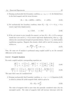
126. 98 Chapter 3. FEM with Magnetostrictive Actuators and Sensors
µσ
increase (decrease) in the ratio of µ
. Similarly the blocked force in the support is
obtained from Equation-(3.48) and is given by
µσ
R1 = −R2 = AdEH1 = AdEIn (3.51)
µ
which is more than the value generally considered (AdEIn). This also depends on
the ratio of permeabilities.
2) For mechanically free boundary condition, where R1 = R2 = 0 (u1 = 0 to remove
rigid body displacement), the Equations (3.48-3.49) are solved to obtain.
H1 = H2 = H = In u2 = LdnI = dnI (3.52)
That is H = In is only true for a free-free boundary conditions. For the other
boundary conditions, the magnitude of magnetic field depends on the ratio of per-
meabilities. Stress σ = E u2 − EdH = 0 which satisfies equilibrium equation of free
L
rod at mechanically free boundary condition.
3) For a sensor with tensile force F and zero coil current (I = 0), where −R1 = R2 = F
(u1 = 0 to remove rigid body displacement).
Fd F Lµ
H1 = H2 = − σ
u2 =
Aµ AEµσ
B = e + µσ H = 0 ⇒ e = −Hµσ (3.53)
Hence again the dependence on the ratio of permeabilities is very important. Stress
F
σ = E − eH = A
which satisfies equilibrium equation.
Hence, It is clear that due to coupling, magnetic field and hence blocked force of a me-
chanically fixed rod is less than the value generally considered in uncoupled model. The
ratio between these two values is calculated for Terfenol-D rod taking data from Terfenol-
D manual [52]. Considering d = 15E − 9 m/amp, E = 30 GPa and constant stress
µσ
relative permeability equal to 10, µ
= 0.46, which is around 50% of the value generally
considered. However, for any other material, if µ d2 E, then µσ ≈µ and uncoupled
and coupled model will give similar result. But for giant magnetostrictive materials like
Terfenol-D, the effect of coupling stiffness matrix is considerable on the axial response.

127. 3.4. Numerical Experiments 99
Sensor Actuator
50mm 50mm
400mm
Degraded Zone
50mm
200mm
500mm
Figure 3.2: Composite Rod With Magnetostrictive Sensor and Actuator
−4
x 10
Uncoupled Healthy
4 Coupled Healthy
Uncoupled Degraded
Coupled Degraded
3
2
Voltage (Volt)
1
0
−1
−2
−3
0 1 2 3 4 5
Time (sec) −4
x 10
Figure 3.3: Open Circuit Voltages at Magnetostrictive Sensor

128. 100 Chapter 3. FEM with Magnetostrictive Actuators and Sensors
3.4.1.3 Degraded Composite Rod with Magnetostrictive Sensor/Actuator
Figure-3.2 shows a composite rod with two magnetostrictive zones, one for actuator and
other for sensor. Between the sensor and actuator location, a small degraded zone of 50
mm dimension is placed. Length of the rod is assumed as 500 mm. Cross sectional area
of the rod is 90mm2 . 50mm long sensor is placed near the support. Actuator of length
50mm is at 400mm apart from support. 200 turns of coils are used in both sensing and
actuation coils. Magnetostrictive actuator is elongated by 5 kHz frequency current (see
Figure-3.6(b)) and magnetostrictive sensor is used to sense the stress wave through the
sensing coil. For the case, when a part of a long composite rod is exposed to chemical
reaction, elastic property of the structure will degrade. This technique can be used to
identify the material degradation zone in the rod. In addition, any change of cross-
sectional area from 10% and up can be identified in rod model, which can be a very cost
effective technique for long-range composite piping inspection.
Figure-3.3 shows the open circuit voltages in the sensor for coupled, uncoupled,
healthy and degraded beam. The degraded zone is modelled by reducing the elastic prop-
erties by 10%. This figure shows that there is a significant difference in the response
between the coupled and uncoupled responses for both healthy and degraded case. How-
ever, the responses for healthy and degraded case vary only marginally at higher time
steps. This is expected since only 10% of the property is degraded. This example clearly
shows the need for coupled formulation.
3.4.2 Finite Element Formulation for a Beam
In this subsection, a shear deformable Finite Element (FE) is deduced from the 3-D FE
formulation. In particular, the effect of stiffness coupling is brought out on the static and
dynamic responses. Mechanical displacement fields are considered as
u(x, y, z, t) = u0 (x, t) − zθx (x, t),
0
v(x, y, z, t) = 0, w(x, y, z, t) = w0 (x, t). (3.54)
Where u, v , w are the components of mechanical displacement at location (x , y, z ) in
X , Y and Z direction (see Figure-3.4) respectively. u 0 and w 0 are the displacement
0
components in mid plane of the composite beam. θx is the slope of the mid plane about
X axis. Magnetic fields in three coordinate directions are
0
Hx (x, y, z, t) = Hxp (x, t), Hy (x, y, z, t) = 0, Hz (x, y, z, t) = 0. (3.55)

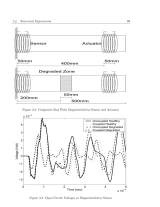
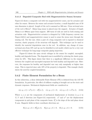
129. 3.4. Numerical Experiments 101
0
Hxp is X directional magnetic field at mid plane of the magnetostrictive patch p. The mag-
netic field along the thickness direction within a particular layer is assumed as constant.
In matrix notation, Equation-(3.54) can be written as
    
 u  1 0 −z  u0 
{U } = v =  0 0 0  w0 ¯
= [Np ]{U } (3.56)
   0 
w 0 1 0 θ
For finite element formulation, displacement and magnetic fields are discretized as
u0 (x) = N1 (x)u1 + N2 (x)u2 w0 (x) = N1 (x)w1 + N2 (x)w2
θ0 (x) = N1 (x)θ1 + N2 (x)θ2 H(x) = N1 (x)H1 + N2 (x)H2 (3.57)
That is each node has four degrees of freedom. Here u1 , u2 , w1 , w2 , θ1 , θ2 are the element
nodal displacements and slopes and H1 , H2 are nodal magnetic fields. Equation-(3.57)
can be written in matrix form as
¯ ¯
{U } = [NU ]{U e } {H} = [NH ]{H e }. (3.58)
Here, nodal mechanical displacement vector, {U e } and magnetic field vector {H e } are
given by
{U e } = {u1 w1 θ1 u2 w2 θ2 }T , {H e } = {H1 H2 }T . (3.59)
The mechanical and magnetic shape functions can be written as
 
N1 0 0 N2 0 0
¯
[NU ] =  0 N1 0 0 N2 0  , [NH ] = N1 N2 (3.60)
0 0 N1 0 0 N2
where linear shape functions are assumed, which are given by
x x
[N1 ] = 1 − , [N2 ] = (3.61)
L L
To formulate mechanical shape function, mechanical displacement {U } can be written
using Equation-(3.56) as
¯
{U } = [Np ][NU ]{U e } = [NU ]{U e } (3.62)
where mechanical shape function [NU ] is
 
N1 0 −zN1 N2 0 −zN2
[NU ] =  0 0 0 0 0 0  (3.63)
0 N1 0 0 N2 0

130. 102 Chapter 3. FEM with Magnetostrictive Actuators and Sensors
¯
The strain displacement matrix [B] can be written from Equation-(3.5) as follows
 
N1,x 0 −zN1,x N2,x 0 −zN2,x
 0 0 0 0 0 0 
 
 0 0 0 0 0 0 
¯
[B] = [L][NU ] =   (3.64)
 0 0 0 0 0 0 
 
 0 N1,x −N1 0 N2,x −N2 
0 0 0 0 0 0
The stiffness matrix [KU U ] can be calculated from Equation-(3.10). To avoid shear locking,
shear part of the [KU U ] matrix is reduced integrated. Values of nonzero elements of
stiffness matrix [KU U ] of a composite laminated beam are the following
A11 A15 A15 B11 A11
K11 = , K12 = , K13 = − , K14 = − ,
L L 2 L L
A15 A15 B11 A55 A55 B15
K15 = − , K16 = + , K22 = , K23 = − ,
L 2 L L 2 L
A15 A55 A55 B15
K24 = − , K25 = − , K26 = + ,
L L 2 L
A55 L D11 A15 B11
K33 = − B15 + , K34 = − + ,
4 L 2 L
A55 B15 A55 L D11 A11 A15
K35 = − + , K36 = − , K44 = , K45 = ,
2 L 4 L L L
A15 B11 A55
K46 = − − , K55 = ,
2 L L
A55 B15 A55 L D11
K56 = − − , K66 = + B15 + ,
2 L 4 L
Kij = Kji [ i, j = 1 to 6].
where Aij , Bij , Dij are
[Aij Bij Dij ] = ¯
Qij [1 z z 2 ]dA (3.65)

131. 3.4. Numerical Experiments 103
The mass matrix [MU U ] can be calculated from Equation-(3.13) and is given by
 
2I0 0 −2I1 I0 0 −I1
 
 0 2I0 0 0 I0 0 
 
 
L  −2I0 0 2I2 −I1 0 I2 
[MU U ] =  . (3.66)
6  I0
 0 −I1 2I0 0 −2I1  
 
 0 I0 0 0 2I0 0 
 
−I1 0 I2 −2I1 0 2I2
where I0 , I1 , I2 are the mass, first moment of mass and second moment of mass per unit
length of the beam and are given by
[I0 I1 I2 ] = ρ[1 z z 2 ]dA (3.67)
A
The matrix [e] in Equations-(2.9) & (2.10) for beam element takes the form as
[e] = e11 0 0 0 0 0 (3.68)
since the magneto-mechanical stress will be experienced only in the axial direction due to
beam bending. The matrix [KU H ] can be calculated from Equation-(3.10) as
T 1 −e0 0 e1 e0 0 −e1
11 11 11 11
[KU H ] = (3.69)
2 −e0 0 e1 e0 0 −e1
11 11 11 11
Where e0 and e1 are given by
11 11
e0
11 e1 =
11 e11 [1 z] dA (3.70)
A
The matrix [KHH ] can be calculated from Equation-(3.16) as
Lµ0 2 1
[KHH ] = (3.71)
6 1 2
Where µ0 is
[µ0 ] = µ dA (3.72)
A
{FH } and {Fv } from Equations-(3.19), (3.31) and (3.35) can be written as
Inµ0 L
{FH }T = 1 1 ,
2
{Fv }T noupled = n
U e0 0 −e1
11 11 −e0 0 e1
11 11 ,
{Fv }T 0r 1r 0r 1r
Coupled = n e11 0 −e11 −e11 0 e11 . (3.73)

132. 104 Chapter 3. FEM with Magnetostrictive Actuators and Sensors
Where e0r and e1r are given
11 11
µσ
e0r
11 e1r
11 = e11 [1 z] dA (3.74)
A µ
3.4.2.1 Composite Beam with Magnetostrictive Bimorph
Numerical simulation is carried out by considering a laminated composite beam of total
thickness 1.8mm as shown in Figure-3.4. Length and width of the beam is 500mm and
50mm respectively. The beam is made of 12 layers with thickness of each layer being
0.15 mm. Surface mounted magnetostrictive patches at the top and bottom layer are
considered as sensor and actuator, respectively. Elastic modulus of composite is assumed
Z
¡
¡ ACTUATOR
¡
¡
¡
MAGNETOSTRICTIVE PATCHES
¡
¡
X
Y
¡
¡
¡
¡
SENSOR
Figure 3.4: Laminated Beam With Magnetostrictive Patches.
as 181 GPa and 10.3 GPa, in the parallel (E1 ) and the perpendicular (E2 ) direction of
fiber. Poisson’s ratio (ν), density (ρ) and shear modulus (G12 ) of composite are assumed
as 0.0, 1.6 gm/c.c. and 28 GPa, respectively. Elastic modulus (Em ), poisson’s ratio
(νm ), shear modulus (Gm ) and density (ρm ) of the magnetostrictive material are taken
as 30 GPa, 0.0, 23 GPa and 9.25 gm/c.c. respectively. Magneto-mechanical coupling
coefficient is taken as 15E-09 m/amp. Permeability at vacuum or air is assumed to be
400 π nano-Henry/m. Constant stress relative permeability of magnetostrictive material
is considered as 10. Number of coil turn per meter (n) in sensor and actuator is assumed
to be 20000. Three different analyses, namely the static, the frequency response and the
time history analysis are performed to bring out the essential difference in the responses
between coupled and uncoupled models.

133. 3.4. Numerical Experiments 105
3.4.2.2 Static Analysis
Table 3.1: Vertical Displacement of Cantilever Tip
Ply Coupled Uncoupled Ratio
Sequence wc mm wu mm wu /wc
m/[0]10 /m 2.17 2.44 1.12
m/[30]10 /m 2.83 3.30 1.17
m/[45]10 /m 3.84 4.78 1.24
m/[60]10 /m 5.52 7.69 1.39
m/[90]10 /m 8.62 15.40 1.78
m/[0/90]5 /m 3.44 4.80 1.40
m/[90/0]5 /m 7.26 10.73 1.48
[m]2 /[0]8 /[m]2 5.25 6.97 1.33
[m]2 /[30]8 /[m]2 6.03 8.41 1.39
[m]2 /[45]8 /[m]2 7.07 10.58 1.50
[m]2 /[60]8 /[m]2 8.53 14.22 1.68
[m]2 /[90]8 /[m]2 10.72 21.56 2.01
[m]2 /[0]4 /[90]4 /[m]2 6.23 10.34 1.66
[m]2 /[90]4 /[0]4 /[m]2 10.77 19.57 1.82
[m]3 /[0]6 /[m]3 8.88 14.39 1.62
[m]3 /[30]6 /[m]3 9.20 15.00 1.63
[m]3 /[45]6 /[m]3 9.62 16.50 1.72
[m]3 /[60]6 /[m]3 10.56 19.40 1.84
[m]3 /[90]6 /[m]3 12.15 25.53 2.10
[m]3 /[0]3 /[90]3 /[m]3 9.00 16.60 1.84
[m]3 /[90]3 /[0]3 /[m]3 12.88 26.31 2.04
[m]4 /[0]4 /[m]4 12.08 23.41 1.93
[m]4 /[30]4 /[m]4 11.48 21.24 1.85
[m]4 /[45]4 /[m]4 11.45 21.15 1.85
[m]4 /[60]4 /[m]4 12.00 23.10 1.93
[m]4 /[90]4 /[m]4 13.3 28.47 2.14
[m]4 /[0]2 /[90]2 /[m]4 11.62 23.10 1.99
[m]4 /[90]2 /[0]2 /[m]4 14.06 30.44 2.17
The effect of coupling of magnetostrictive material in a laminated composite beam
for static actuation is analyzed for 1 Amp DC actuation coil current. It is observed that
tip deflection for coupled analysis is 2.17mm, where as for uncoupled analysis, it is found
to be 2.44mm. The ratio between these two is 1.12. As the thickness of the actuator is
less compared to the thickness of the composite beam, the effective increase of stiffness
in the global stiffness matrix due to coupling is very less. Increase of thickness of sensor

134. 106 Chapter 3. FEM with Magnetostrictive Actuators and Sensors
and actuator patches will increase the effective thickness and hence decrease the effective
deflection, especially in the coupled analysis. In addition, increase of ply angle will also
increase the stiffness in the transverse direction. This aspect is shown in Table-3.1 for
different ply angles range from 00 to 900 . It is very clear from the table that for 900
ply angle, the effect of coupling is considerable. This reinforces the need for coupled
analysis for structures with magnetostrictive patches. In the next two analyses, the effect
of coupling in dynamic analysis in the context of structural health monitoring is further
emphasized.
3.4.2.3 Frequency Response Analysis of a Healthy and Delaminated Beam
In the FE modelling, delamination in the composite beam is modelled using two sub-
laminates, one for top and other for bottom part of the delamination. Stiffness or mass
matrices of the elements for top sub-laminate are integrated from the delaminated layer to
the top layer and for the bottom sub-laminate, from the bottom layer to the delaminated
layer. FE nodes for top sub-laminate are only connected with the elements for top sub-
laminate and similarly, nodes for bottom sub-laminate are connected with the elements for
bottom sub-laminate. Physical locations of these two sets of FE nodes are in the neutral
axis of the original beam. Hence, two nodes will exist in the delaminated zones, one for
elements of top sub-laminate and other for elements of bottom sub-laminate. These two
nodes are not directly connected with any element. Detail modelling of delamination is
explained in section-6.2 with examples and with Figure-6.1.
To observe the effects of coupling terms of magnetostrictive material in the frequency
domain, frequency response function (FRF) is calculated with both coupled and uncoupled
model for the same cantilever composite beam up to 3rd natural frequencies. FRF for 00
and 900 ply angle is shown in Figure-3.5(a) and Figure-3.5(b) respectively. For 00 ply
angle, we see that the first two modes are least effected due to the effect of coupling.
However, we can see significant shift in resonant frequency of higher modes. For the 900
ply angle, one sees the shift in the natural frequencies even for first mode. This farther
reinforces our belief that uncoupled analysis under estimate the stiffness of the structure
with magnetostrictive material. From the structural health monitoring point of view, the
difference in the responses between the healthy and the damaged structures indicate the
presence of the defect. FRFs for the same beam with 100mm mid layer delamination
at 100mm apart from support are also shown in the same figures for both coupled and
uncoupled material model. In both the figures, it is observed that, the higher modes

135. 3.4. Numerical Experiments 107
0
10
−2
10
Abs(H(ω))
−4
10
−6
10
Uncoupled Healthy
Coupled Healthy
Uncoupled Delaminated
−8
10 Coupled Delaminated
0 50 100 150
Frequency (Hz)
(a) 00 ply angle
0
10
−2
10
Abs(H(ω))
−4
10
−6
10
Uncoupled Healthy
Coupled Healthy
10
−8 Uncoupled Delaminated
Coupled Delaminated
0 10 20 30 40 50 60 70
Frequency (Hz)
(b) 900 ply angle
Figure 3.5: Frequency Response Function

136. 108 Chapter 3. FEM with Magnetostrictive Actuators and Sensors
are slightly affected while the initial modes are affected least. In addition, the damage
sensitivity in the FRF of the structure is less than the error due to uncoupled assumption of
analysis. Yet another parameter where the effect of coupled analysis requires investigation
is the frequency of the AC current required to generate the magnetic field. This can be
seen from the time history analysis, which is given in next subsection.
3.4.2.4 Time Domain Analysis
To observe the effects of coupled analysis on structure with magnetostrictive material,
time domain analysis is carried out for both low and high frequency actuation for the
same cantilever composite beam. Here, the structure is actuated through a sinusoidal
time signal current, I of 0.5 amp amplitude AC current (I0 ) and 0.5 Amp bias current
(IDC ) at 50 Hz and 5 kHz frequency, respectively. The equation of current is given by
I = I0 sin(ωt) + IDC (3.75)
These are shown in Figure-3.6(a) and Figure-3.6(b) respectively. Direct transient dynamic
analysis is performed for 200 time steps to calculate open circuit voltage of the sensor
and beam tip velocity. Each time step is 50 mili-seconds and 5 micro-seconds for 50 Hz
and 5 kHz actuation, respectively. Figure-3.7(a) and Figure-3.7(b) shows the tip velocity
of the cantilever beam for 50 Hz and 5 kHz respectively with 00 ply angle. From these
figures, we see that the effect of magneto-mechanical coupling is negligible for both low
and high actuation frequency. But sensitivity of delamination in the responses is more
in high frequency than low frequency actuation. Figure-3.8(a) and Figure-3.8(b) shows
the tip velocity of the cantilever beam for 50 Hz and 5 kHz respectively with 900 ply
angle. However, with 900 degree ply angle, we can start seeing the difference in behavior
for actuation frequencies 50 Hz and 5kHz. For low frequency actuation, coupling has
phenomenal effect. At high frequency actuation, there is no period error. However,
coupling introduces lower velocity amplitudes.
Figure-3.7(a) and Figure-3.8(a) show high frequency signal at the start of the re-
sponse. To avoid double frequency effect in magnetostrictive actuator, windowed sinu-
soidal current amplitude is biased with DC current, which has both low frequency as well
as high frequency component. In addition, open circuit voltages in sensors are propor-
tional to the time derivative of the stress integrated along the length of the sensor. Initial
high frequency signals are due to these extra complicacies of the sensing and actuation
calculation, when sensor and actuator exists in the same element of the finite element

137. 3.4. Numerical Experiments 109
FFT of Current History
100
Coil Current History
90 1
80 Actuation Current (Amp)
0.8
70
Frequency Content
0.6
60
50 0.4
40
0.2
30
0
20 0 0.02 0.04 0.06 0.08 0.1
Time (sec)
10
0
0 100 200 300 400 500
Frequency (Hz)
(a) 50Hz Actuation
FFT of Current History
100
Coil Current History
90 1
80
0.8
Actuation Current (Amp)
70
Frequency Content
60 0.6
50 0.4
40
0.2
30
20 0
0 0.2 0.4 0.6 0.8 1
Time (sec) −3
x 10
10
0
0 10 20 30 40 50
Frequency (KHz)
(b) 5 kHz Actuation
Figure 3.6: Actuation History with Frequency content

138. 110 Chapter 3. FEM with Magnetostrictive Actuators and Sensors
UnCoupled Healthy
0.4 Coupled Healthy
UnCoupled Delaminated
Coupled Delaminated
0.3
0.2
Velocity (m/Sec)
0.1
0
−0.1
−0.2
−0.3
0 0.02 0.04 0.06 0.08 0.1
Time (Sec)
(a) 50Hz Actuation
UnCoupled Healthy
Coupled Healthy
0
UnCoupled Delaminated
Coupled Delaminated
−0.01
−0.02
Velocity (m/Sec)
−0.03
−0.04
−0.05
−0.06
−0.07
0 0.2 0.4 0.6 0.8 1
Time (Sec) x 10
−3
(b) 5 kHz Actuation
Figure 3.7: Cantilever Tip Velocity for 00 ply angle

139. 3.4. Numerical Experiments 111
analysis. From the responses of delaminated beam in above figures, it is emphasizing the
requirement of coupled analysis for structural health monitoring application.
Figure-3.9(a) and Figure-3.9(b) shows the open circuit voltages generated in the
sensory patches for low and high frequency actuating current for 00 ply angle laminate.
The effect of coupling and damage are almost negligible. However, coupling effect induces
significant changes in the voltages for 900 ply angle laminate. Figure-3.10(a) shows the
open circuit voltages with 900 ply angle laminate for 50 Hz actuation. The figure shows
that the delamination increases the open circuit voltages in uncoupled analysis, while it
decreases in the coupled analysis. Figure-3.10(b) shows the open circuit voltages with 900
ply angle for 5 kHz actuation. Differences between the open circuit voltages considering
coupled and uncoupled formulation are considerable.
These examples show that the uncoupled model of the laminated composite struc-
ture with magnetostrictive patches in most cases gives upper bound solutions, which is
highly non-conservative from the structural design point of view. In addition, for struc-
tural health monitoring application, the difference in response between the healthy and
damaged beam is found significant in the coupled analysis. These studies justify the need
for coupled material model for realistic analysis of composite beams with magnetostrictive
material patches.
3.4.3 Finite Element Formulation of a Plate
In this subsection, a cantilever plate element with magnetostrictive material patches de-
duced from the generalized 3-D formulation discussed earlier is studied. The element is
based on first order shear deformation theory (Mindlin’s theory). Further, this element is
used to model a plate with multiple delaminations and the effect of coupled and uncoupled
model on the responses of the healthy and delaminated plate is investigated. Mechanical
displacement fields can be written as
u(x, y, z, t) = u0 (x, y, t) − zθx (x, y, t),
0
v(x, y, z, t) = v 0 (x, y, t) − zθy (x, y, t),
0
w(x, y, z, t) = w0 (x, y, t). (3.76)
Where u, v , w are the components of mechanical displacement at location (x , y, z ) in X , Y
and Z direction respectively. u 0 , v 0 and w 0 are the displacement components in mid plane
0 0
of the composite plate. θx and θy are the slope of the mid plane about X and Y axis

140. 112 Chapter 3. FEM with Magnetostrictive Actuators and Sensors
0.4
0.3
0.2
0.1
Velocity (m/Sec)
0
−0.1
−0.2
−0.3
−0.4
UnCoupled Healthy
Coupled Healthy
−0.5
UnCoupled Delaminated
Coupled Delaminated
−0.6
0 0.02 0.04 0.06 0.08 0.1
Time (Sec)
(a) 50Hz Actuation
UnCoupled Healthy
0 Coupled Healthy
UnCoupled Delaminated
Coupled Delaminated
−0.02
−0.04
Velocity (m/Sec)
−0.06
−0.08
−0.1
−0.12
−0.14
−0.16
0 0.2 0.4 0.6 0.8 1
Time (Sec) x 10
−3
(b) 5 kHz Actuation
Figure 3.8: Cantilever Tip Velocity for 900 ply angle.

141. 3.4. Numerical Experiments 113
0.2 UnCoupled Healthy
Coupled Healthy
UnCoupled Delaminated
0.15 Coupled Delaminated
0.1
0.05
Voltage (volt)
0
−0.05
−0.1
−0.15
−0.2
0 0.01 0.02 0.03 0.04 0.05 0.06 0.07 0.08 0.09
Time (Sec)
(a) 50Hz Actuation
5
4
3
2
Voltage (volt)
1
0
−1
−2
−3 UnCoupled Healthy
Coupled Healthy
−4 UnCoupled Delaminated
Coupled Delaminated
0 1 2 3 4 5 6 7 8 9
Time (Sec) −4
x 10
(b) 5 kHz Actuation
Figure 3.9: Sensor Open Circuit Voltage for 00 ply angle

142. 114 Chapter 3. FEM with Magnetostrictive Actuators and Sensors
0.5
0.4
0.3
0.2
Voltage (volt)
0.1
0
−0.1
−0.2
−0.3
UnCoupled Healthy
−0.4 Coupled Healthy
UnCoupled Delaminated
−0.5 Coupled Delaminated
0 0.01 0.02 0.03 0.04 0.05 0.06 0.07 0.08 0.09
Time (Sec)
(a) 50Hz Actuation
10
5
Voltage (volt)
0
−5
UnCoupled Healthy
Coupled Healthy
−10 UnCoupled Delaminated
Coupled Delaminated
0 1 2 3 4 5 6 7 8 9
Time (Sec) −4
x 10
(b) 5 kHz Actuation
Figure 3.10: Sensor Open Circuit Voltage for 900 ply angle

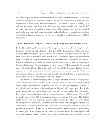
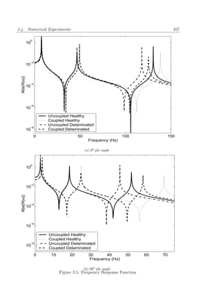
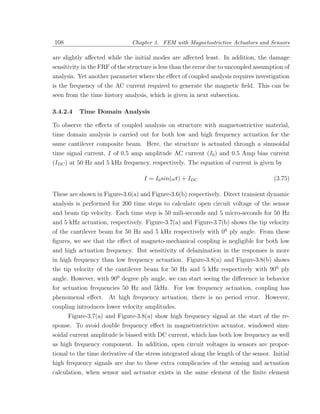
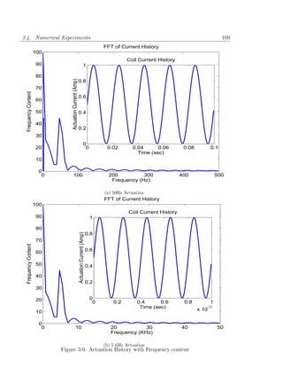
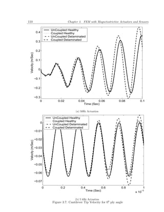
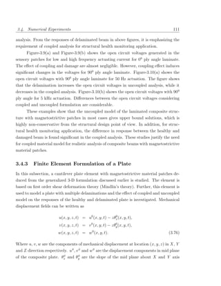
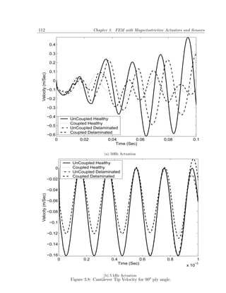
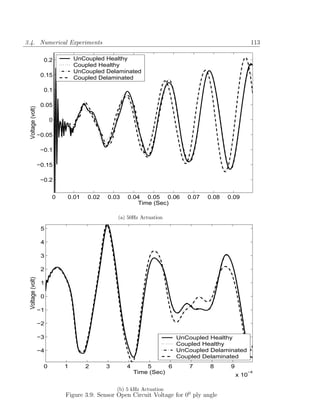
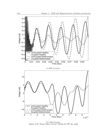
143. 3.4. Numerical Experiments 115
respectively. Magnetic fields in three coordinate directions are assumed as
0 0
Hx (x, y, z, t) = Hxp (x, y, t), Hy (x, y, z, t) = Hyp (x, y, t), Hz (x, y, z, t) = 0. (3.77)
0 0
Hxp and Hyp are X and Y directional magnetic field at mid plane of the magnetostrictive
patch p respectively. Hence, the magnetic field along the thickness direction within a
particular layer is assumed as constant. In matrix notation, Equation-(3.76) can be
written as
 0 
     u0 

 
 u  1 0 0 −z 0  v 
 

{U } = v =  0 1 0 0 −z  w 0 ¯
= [Np ]{U } (3.78)
   0 
 θx 
w 0 0 1 0 0 
 0 
 
θy
Stiffness and mass matrices of plate element are derived using bilinear shape functions
with standard 4 noded finite element formulation. Here each node of the element has
seven degrees of freedoms (five mechanical and two magnetic degrees of freedom).
Delamination for plate in finite element modelling is performed similar to the beam
as discussed in previous section. For single delamination, delaminated zone is modelled
with two sets of elements, one for top sub-laminate and other for bottom sub-laminate of
the plate. Two sets of nodes are also generated, where only one set is connected with the
elements for top sub-laminate and other set is connected with the elements for bottom
sub-laminate. Physical location of these nodes are in the neutral plane of the plate,
which may differ from the mid plane of these individual sub-laminates. Undelaminated
zone is modelled with single set of elements and nodes. These nodes are in the neutral
plane of the plate. Interface of the delaminated and undelaminated zone is modelled
with merging the nodes, which are physically in the same place. However, two nodes for
two sub-laminates and one node for undelaminated laminate are merged in the interface
of the delamination for the integrity of the model. For multiple delaminations, similar
approach is taken for every delamination one by one in the model. However, where the
delaminations are overlapped, more number of sub-laminates are required. Every sub-
laminate is modelled with plate elements, where stiffness and mass matrices for these
elements are calculated according to their location and thickness with respect to the
neutral plane of the plate. For each sub-laminate, a set of nodes are generated according
to the size of the delaminations, which are connected only with the elements for the
respective sub-laminate. At the periphery of the each delamination, respective nodes

144. 116 Chapter 3. FEM with Magnetostrictive Actuators and Sensors
are merged with the nodes of sub-laminates, which are just below and above of the
delamination.
3.4.3.1 Composite Plate with Magnetostrictive Sensor and Actuator
Numerical simulation is carried out by considering a laminated composite plate of total
thickness 1.8mm as shown in Figure-3.11. Length and width of the beam is 500mm
and 500mm respectively. The beam is made of 12 layers with thickness of each layer
being 0.15 mm. Surface mounted magnetostrictive patches at the top and bottom layer
are considered as actuator and sensor, respectively. Dimension of sensor and actuator
are 100mm X 100mm and at the center of plate. Three center delaminations of size,
100mmX100mm, 200mmX200mm and 300mmX300mm are considered to study the effect
of multiple delaminations in the response of structure. These delaminations are assumed
just above the sensor, to block the direct stress waves from actuator to sensor. The FE
modelling is done with the plate elements of 10 mm X 10 mm size. Solution is performed
by Newmark time integration with 100 time steps.
Figure-3.12 shows the open circuit voltages for 50Hz actuation. Effect of coupling
is less dominant than the effect of delamination, as the plate is severely damaged.
3.4.4 Finite Element Formulation of 2D Plane Strain Elements
In this subsection, as before, a 2-D plane strain Finite Element (FE) is deduced from
the 3-D FE formulation. This element is then used to model different types of failures,
namely the fiber breakages, internal cracks and matrix cracks. The main aim, as before, is
to study the sensitivity of the response due to coupled and uncoupled model. Mechanical
displacement fields can be written as
u(x, y, z, t) = u0 (x, z, t), v(x, y, z, t) = 0, w(x, y, z, t) = w0 (x, z, t), (3.79)
where u, v , w are the components of mechanical displacement at location (x , y, z ) in X , Y
and Z direction respectively. u 0 and w 0 are the displacement components of the beam
and depends on x , z and t. Magnetic fields in three coordinate directions are assumed as
0 0
Hx (x, y, z, t) = Hxp (x, z, t), Hz (x, y, z, t) = Hzp (x, z, t), Hy (x, y, z, t) = 0, (3.80)
0 0
where, Hxp and Hzp are X and Z directional magnetic field of the magnetostrictive patch
p respectively. The mechanical displacements and magnetic field component along the

145. 3.4. Numerical Experiments 117
Actuator
100mm
100mm
m
0m
50
Actuator
1.8 mm
Multiple Delamination
Sensor
100mm
200mm
300mm
500mm
Figure 3.11: Multiple delaminated plate with magnetostrictive sensor and actuator
0.01
0.008
0.006
0.004
Voltage (volt)
0.002
0
−0.002
−0.004
−0.006
UnCoupled Healthy
Coupled Healthy
−0.008 UnCoupled Delaminated
Coupled Delaminated
−0.01
0 0.01 0.02 0.03 0.04 0.05 0.06 0.07 0.08 0.09
Time (Sec)
Figure 3.12: Sensor open circuit voltage for plate with multiple delaminations

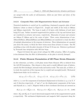
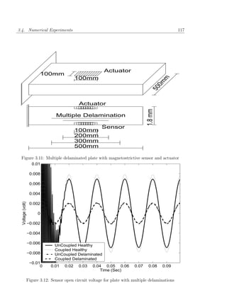
146. 118 Chapter 3. FEM with Magnetostrictive Actuators and Sensors
width direction are assumed equal to zero. Stiffness and mass matrices for 2D plane
strain element are derived using 4 noded bilinear shape functions with standard finite
element formulation. Here each node of the element has four degrees of freedoms (two
mechanical and two magnetic degrees of freedom).
3.4.4.1 Composite Beam with Different Types of Failure
Numerical simulation is carried out by considering a laminated cantilever composite beam
of total thickness 20mm as shown in Figure-3.13. Length and width of the beam is 250mm
and 50mm respectively. The beam is made of 4 layers ([0/45/ − 45/90]) with thickness of
each layer being 5 mm. Surface mounted magnetostrictive patches at the top and bottom
layer are considered as sensor and actuator, respectively. 50mm X 50mm X 5mm size
sensor and actuator are placed near the support and 150mm apart from the support of
the cantilever, respectively. Beam is modelled with 250 X 20 numbers of 4 noded plane
strain elements with each size of 1 mm X1 mm. Thickness of the crack in FE modelling is
assumed as 1 mm. Figure-3.13(a) shows the 5mm matrix cracking at 100 mm apart form
the support. Matrix cracking in FE formulation is modelled by removing elements (5
numbers) from the location of the crack in the layer of 900 ply angle. Actuator is excited
with 5kHz actuation. Figure-3.14 shows the open circuit voltages for this matrix cracking.
Effect of matrix cracking is less sensitive than the error due to uncoupled material analysis.
The stiffness loss at 900 layer is less compared to the 00 layer. Figure-3.13(b) shows the
5mm fiber breakage at 100mm apart form the support. Fiber breakage in FE formulation
is modelled by removing elements (5 numbers) from the location of the crack in the layer
of 00 ply angle. Figure-3.15 shows the open circuit voltages for this fiber breakage. Effect
of fiber breakage is more sensitive than the error due to uncoupled material analysis.
The stiffness loss at 00 layer is more compared to 900 layer in this case. Open circuit
voltages are more for damaged structure than undamaged structure for both coupled and
uncoupled formulation. Figure-3.13(c) shows the 10mm center crack at 100mm apart
form the support. Center crack in FE formulation is modelled by removing elements (10
numbers) from the location of the crack. Figure-3.16 shows the open circuit voltages for
this internal crack. In this case, the figure shows that the effect of damage and coupled
formulation are comparable.

147. 3.4. Numerical Experiments 119
5mm
(a) Matrix Cracking
50mm
0
45
−45
90
(b) Fiber Breakage
50mm
10mm
20mm
Sensor Actuator
100mm 50mm 50mm
250mm
(c) Internal Crack
Figure 3.13: Laminated composite beam with sensor, actuator and crack
1 UnCoupled Healthy
Coupled Healthy
0.8 UnCoupled Mid Crack
Coupled Mid Crack
0.6
0.4
Voltage (volt)
0.2
0
−0.2
−0.4
−0.6
−0.8
−1
0 0.5 1 1.5 2 2.5 3
Time (Sec) x 10
−4
Figure 3.14: Sensor open circuit voltages for matrix crack in laminated composite beam

148. 120 Chapter 3. FEM with Magnetostrictive Actuators and Sensors
UnCoupled Healthy
Coupled Healthy
UnCoupled Fib Breakage
1 Coupled Fib Breakage
0.5
Voltage (volt)
0
−0.5
−1
0 0.5 1 1.5 2 2.5 3
Time (Sec) x 10
−4
Figure 3.15: Sensor Open Circuit Voltages for Fiber Breakage
UnCoupled Healthy
Coupled Healthy
UnCoupled Int. Crack
1 Coupled Int. Crack
0.5
Voltage (volt)
0
−0.5
−1
0 0.5 1 1.5 2 2.5 3
Time (Sec) x 10
−4
Figure 3.16: Sensor Open Circuit Voltages for Internal Crack

149. 3.5. Summary 121
3.5 Summary
This study is mainly intended to bring out the importance of coupled model over uncou-
pled model in the analysis of smart composite structures with magnetostrictive patches
and its effect on the structural health monitoring application. Coupled model is stud-
ied without assuming any direct relationship of magnetic field unlike uncoupled model.
Here, elastic modulus, permeability and magneto-mechanical strain coefficient is consid-
ered as constant matrix. Actuation and sensing both has been done using actuation and
sensing coil arrangement. Mechanical displacement and magnetic fields are considered
as mechanical degrees of freedoms and smart degrees of freedoms respectively for finite
element formulation. Thus both sensor and actuator coil properties can be incorporated
with in the frame work of the finite element formulation. Numerical results have shown
that coupling is quite significant for 900 ply angle and quite insignificant in a 00 laminate.
Also, coupling is shown to be significant for low actuation frequency. It has been observed
that the effect of coupling in static analysis is around 12% and is shown to increase with
the thickness of the actuator. It is observed that for structural health monitoring appli-
cation, coupled analysis is essential to get the true response of structure. However, when
the damage is severe, simplified uncoupled analysis can still be used to get a preliminary
solution.

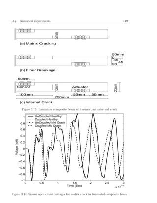
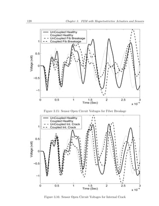
150. Chapter 4
Superconvergent Beam Element with
Magnetostrictive Patches
4.1 Introduction
In the last chapter, a series of Finite Element (FE) formulation were performed and these
were applied to solve some health monitoring problems involving different flaws such as
material degradation, delamination, fiber breakages, matrix cracking etc. In most cases,
substantial flaw sizes were considered to induce a voltage change in the sensing coil.
However, if the flaw size is very small, then one would require signal with high frequency
content. From FE point of view, such a signal will enormously increase the problem sizes
due to the requirement that the element size be comparable to the wavelength, which are
very small at high frequencies. This problem can be alleviated to a certain level by using,
what is known as super-convergent FE formulation.
One of the fundamental problems encountered in FE formulation is choice of appro-
priate polynomials of the field variable. For example, for obtaining accurate responses for
the field variable (transverse displacement) in elementary beam, one needs a cubic poly-
nomial, and the formulated element using such polynomial is a C 1 continuous element
as it has to satisfy both displacement and slope continuity. On the other hand, for the
same beam, if shear deformation is considered, this slope is independently interpolated
along with transverse displacement and both these field variables require only linear poly-
nomials. In other words, the formulation is C 0 continuous. If such an element is used
in this beam situation, where the shear strains are negligible, the element’s response will
be many orders smaller than the true response. This phenomenon is called the ”Shear
locking problem” and so far is dealt in many references [313, 314, 427, 325, 32, 123, 347].
Normally one under-integrates the energy terms associated with the shear stress/strain
122

151. 4.1. Introduction 123
[313] to remove the locking. Alternatively, one can use the superconvergent solution to
the governing equation as interpolating function for element formulation. This completely
removes locking and some of the constants of the interpolating functions become mate-
rial/sectional properties dependent. In this approach, the static part of the governing
equation is exactly solved and used as interpolating function for element formulation.
Hence, the approach gives exact static stiffness for point loads. Some of the constants
in the interpolating function, when evaluated in term of nodal displacements, become
dependent on material/sectional properties of the beam.
4.1.1 Existing Literature
Such approaches were adopted to develop elements for Herman-Mindlin rod [139], first-
order shear deformable composite beam [62], first- and higher-order shear deformable
isotropic beam [181, 325] and beam with Poisson’s contraction [64]. Chakraborty et al.
[63] developed such an element for functionally graded beam based on first order shear
theory. Mitra et al. [268] developed super convergent element of arbitrary cross-section
for composite thin wall beam with open or closed contour. Superconvergent solution
for bending of isotropic beam based on higher order shear deformable theory (HSDT)
was reported by Eisenberger [114]. Similar solutions for the bending of thin and thick
cross-ply laminated beams were presented by Khedir and Reddy [180, 181] using the state
space concept. Murthy et al. [283] developed a refined higher order finite element for
asymmetric composite beams.
In this chapter, the super-convergent FE approach is used to derive two different
beam elements with embedded magnetostrictive patches, one for Euler-Bernoulli beam
and the other for a shear deformable beam. As a result, in most cases, only a single
element is adequate to capture the static behavior irrespective of boundary conditions
and ply-stacking configuration. As seen in the previous works, the coefficients associated
with the interpolating polynomial are expected to be dependent on the material properties
and the ply-stacking sequence. Finally these super-convergent elements will be used for
material property identification using an Artificial Neural Network (ANN) model, where a
number of finite element simulation is essential with different values of material properties
to generate a mapping relation between structural response and material properties. These
finite element simulations can be performed using very few formulated super-convergent
elements, which can simultaneously reduce the computational time. Again, here, the
elements will be formulated for both uncoupled and coupled material models and their

152. 124 Chapter 4. Superconvergent Beam Element with Magnetostrictive Patches
effects on the response will be brought out in most of the examples solved in this chapter.
This chapter is organized as follows. First the variational formulation is presented
to obtain the governing differential equations of Euler-Bernoulli and first order shear
deformable beam. Both coupled and uncoupled constitutive models are discussed. This
is followed by a section on numerical experiments, where, static and free vibration results
are presented. This section concludes with an example that demonstrates the utility of
this element in material property identification of magnetostrictive material through both
polynomial and artificial neural network identification. The findings in this chapter are
summarized at the end.
4.2 Super-Convergent Finite Element Formulations.
In this section, developments of two different finite elements are outlined: one based on
the elementary (Bernoulli-Euler) theory and the other based on First order Shear Defor-
mation (Timoshenko) theory. For each of these elements, FE model based on coupled and
uncoupled properties of constitutive model of the magnetostrictive material, are formu-
lated.
4.2.1 FE Formulation for Euler-Bernoulli Beam.
The foremost requirement for formulating super convergent elements is to derive the
governing differential equation of the system. We do this here using Hamilton’s principle.
The displacement and magnetic field variation for the element is assumed as:
U (x, y, t) = u◦ (x, t) − zw,x (x, t),
◦
V (x, y, t) = 0, (4.1)
W (x, y, t) = w◦ (x, t),
Hx (x, y, t) = Hxp (x, t),
where U, V, W are the mechanical displacements in the three coordinate directions, u◦ and
w◦ are the mid plane displacements of the laminate. The Hx is the magnetic field in the x
direction, while Hxp is the magnetic field in the pth patches. To handle magneto-thermo-
mechanical analysis, we include the thermal variation in the strain distribution and it is
given by
∂U
xx = x
◦
= u◦ − zw,xx − α(∆T ), (4.2)
∂x

153. 4.2. Super-Convergent Finite Element Formulations. 125
where α is the coefficient of thermal expansion and (∆T ) is the temperature rise. The
constitutive relation for the beam with magnetostrictive patches is given by
¯
σxx = Q11 xx − e11 H, Bxx = e11 xx + µ H, (4.3)
where σxx and xx ,
are normal stresses and normal strains in the x direction. The Bxx is the
¯
magnetic flux density in the x direction. Also Q11 is the material constant for mechanical
loads, while e11 and µ are magnetostrictive stress coefficient and strain permeability of the
magnetostrictive material, respectively. In above expression, H = Hxp is the magnetic
field, which is basically the unknown for coupled constitutive model, and is equal to
H = nI for the uncoupled constitutive model, where I is coil current and n is the coil
turn per unit length.
The strain energy (S), the energy due to magnetic field (Wm ) and kinetic energy
(T ) are then given by
L
1
S= (σxx εxx ) dA dx , (4.4)
2 0 A
L
1
Wm = ( Bxx H + Inµσ H) dA dx , (4.5)
0 A 2
1 L ˙2 ˙2
T = (z)(U + W ) dA dx , (4.6)
2 0 A
where µσ is the permeability measured at constant stress. Here (˙) denotes the time
derivative; (z), L and A are the density, the length and the area of cross-section of the
beam, respectively. Applying Hamilton’s principle, we get the following three governing
equations corresponding to 3 degrees of freedom:
δu◦ : ¨ ¨◦
I0 u◦ − I1 w,x + A11 u◦ − B11 w,xxx −
,xx
◦
Ae Hxp,x = 0,
11p
p
δw :◦ ¨
I0 w ◦ + B11 u◦
,xxx − ◦
D11 w,xxxx − e
B11p Hxp,xx = 0, (4.7)
p
δHxp : Ae u◦ − B11p w,xx + Aµp Hxp − Inp Aσ − Aeα (∆T ) = 0.
11p ,x
e ◦
µp 11p
The associated three force boundary conditions are
N = −A11 u◦ + B11 w,xx +
,x
◦
Ae Hxp + Aα ∆T ,
11p 11
p
M = B11 u◦ − D11 w,xx −
,x
◦ e α
B11 Hxp − B11 ∆T , (4.8)
p
V = −B11 u◦
,xx + ◦
D11 w,xxx + e
B11p Hxp,x ,
p

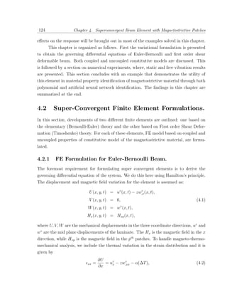
154. 126 Chapter 4. Superconvergent Beam Element with Magnetostrictive Patches
where N is the axial force, M is the moment and V is the shear force. The cross sectional
properties Aij , Bij , Dij , Ae , Bijp , I0 , I1 , I2 , Aµp and Aσ are given by
ijp
e
µp
[Aij Bij Dij ] = ¯
Qij [1 z z 2 ]dA, (4.9)
A
ijp
e
[Ae Bijp ] = eij [1 z]dA, (4.10)
p
[I0 I1 I2 ] = ρ[1 z z 2 ]dA, (4.11)
A
[Aµp Aσ ] =
µp [µ µσ ]dA. (4.12)
p
In the above expression, the integration over p means that this operation is performed
only to pth magnetostrictive layer. The cross-sectional thermal stiffness is given by
Aα α
Bij = ¯
αQij [1 z] dA. (4.13)
ij
4.2.1.1 Uncoupled Formulation
For finite element beam formulation based on uncoupled constitutive model, we have
Hxp = H = nI, ∂Hxp /∂x = 0. Hence, the governing equations and the associated bound-
ary conditions become
δu◦ : ¨ ¨◦
I0 u◦ − I1 w,x + A11 u◦ − B11 w,xxx = 0,
,xx
◦
δw◦ : ¨
I0 w◦ + B11 u◦ − D11 w,xxxx = 0,
,xxx
◦
(4.14)
and
N = −A11 u◦ + B11 w,xx +
,x
◦
Ae Hxp + Aα ∆T ,
11p 11
p
M = B11 u◦
,x − ◦
D11 w,xx − e α
B11 Hxp − B11 ∆T , (4.15)
p
V = −B11 u◦
,xx + ◦
D11 w,xxx .
It is to be noted that the magnetic field will appear only in the force boundary conditions.
The FE equation begins by solving Equation (4.14) exactly. Taking only the static parts
of the Equation-(4.14) and simplifying, we can write it as
u◦ = 0,
,xxx
◦
w,xxxx = 0. (4.16)

155. 4.2. Super-Convergent Finite Element Formulations. 127
The solutions of Equation-(4.16), are:
u◦ = c0 + c1 x + c2 x2 , w◦ = c3 + c4 x + c5 x2 + c6 x3 , (4.17)
where c0 , c1 , c2 , c3 , c4 , c5 , c6 are seven unknown constants to be determined from six nodal
degrees of freedom (u◦ , w◦ , φ = ∂w◦ /∂x at the two nodes). Thus, there must be one
dependent constant, which can be obtained by substituting Equation-(4.17) in Equation-
(4.14) and Equation-(4.15). Introducing a variable βe as
B11
βe = 3 ,
A11
and substituting u◦ and w◦ in the static part of the governing differential equations
(Equation-(4.14)), we get c2 = βe c6 . Hence, the modified displacement fields can now
be written as
u◦ = c0 + c1 x + βe c6 x2 , w◦ = c3 + c4 x + c5 x2 + c6 x3 . (4.18)
For symmetric ply lay up, Bij = 0 and hence βe = 0. In this case axial and transverse
deformation gets uncoupled and the interpolation function reduces to that of simple rod
and Euler-Bernoulli beam, respectively. Equation-(4.18) can now be written in matrix
notation as
{u◦ w◦ w,x }T = [N (x)]{C},
◦
(4.19)
where [N (x)] is a matrix of dimension 3X6, which contains functions of x, i.e., x, x2 and
x3 . The unknown constant vector {C} is given by
{C} = {c0 c1 c3 c4 c5 c6 }T . (4.20)
First we relate the nodal degrees of freedom to the unknown constants by the definitions:
u◦ (x = 0) = u◦ ,
1 w◦ (x = 0) = w1 ,
◦
φ◦ (x = 0) = φ◦ ,
1
u◦ (x = L) = u◦ ,
2 w◦ (x = L) = w2 ,
◦
φ◦ (x = L) = φ◦ ,
2 (4.21)
which can be written in matrix notation as
{ue } = {u◦
1
◦
w1 φ◦
1 u◦
2
◦
w2 φ◦ }T = [G−1 ]{C},
2 (4.22)
and inverting this, we get
{C} = [G]{ue }. (4.23)

156. 128 Chapter 4. Superconvergent Beam Element with Magnetostrictive Patches
Now this vector {C} is substituted in the Equation-(4.19) to get the mechanical displace-
ment for any arbitrary location in terms of nodal displacements {ue } as
{u◦ w◦ w,x }T = [N (x)][G]{ue }
◦ ¯
= [N (x)]{ue }, (4.24)
¯
where [N (x)] is the shape function matrix for mechanical degrees of freedom and are given
in Appendix-A. To obtain the stiffness matrix, forced boundary conditions (Equation-
(4.15)) are used where, Hxp and (∆T ) terms are used to get the equivalent nodal force
due to coil current and temperature rise respectively. Substituting the displacement field
from Equation-(4.18), the force resultants in Equation-(4.15) can be written in terms of
the unknown constants {C} as
{N V ¯
M }T = [G]{C} + {R}. (4.25)
Substituting the expression of {C} from Equation-(4.23), Equation-(4.25) can be written
as
{N V ¯
M }T = [G][G]{ue } + {R}. (4.26)
Evaluating Equation-(4.26) at x = 0 and x = L, we get the nodal load vector, {F } in
terms of nodal displacement {ue }, which can be written as
{F } = {−N (0) − V (0) − M (0) N (L) V (L) M (L)}T
¯
GG(x = 0) {R}(x = 0)
= ¯ {ue } + (4.27)
GG(x = L) {R}(x = L)
= [K]{ue } + {RT }(∆T ) + {RI }Inp ,
p
where [K] is the element stiffness matrix. {RT } and {RI } are element load vector coef-
ficient due to temperature rise and current actuation respectively. Explicit forms of [K],
{RT } and {RI } are given in Appendix A.
Next, the consistent element mass matrix [M ] is derived. It can be computed from
the expression:
L
[M ] = ˆ ˆ
([N (x)]T [ ][N (x)])dAdx, (4.28)
0 A
ˆ
where [N (x)] is another shape function, which can be calculated from longitudinal shape
¯
function [N (x)] as
 
1 0 −z
ˆ ¯
[N (x)] =  0 0 0  [N (x)]. (4.29)
0 1 0

157. 4.2. Super-Convergent Finite Element Formulations. 129
The nonzero elements of the mass matrix are given in Appendix-A. Mass and stiffness
matrices for conventional element can be calculated considering βe = 0. After finite ele-
ment solution, from the strain and the magnetic field, stress and magnetic flux density
can be calculated using Equation-(4.3).
4.2.1.2 Coupled Formulation
For finite element beam formulation based on coupled constitutive model, magnetic field
terms Hxp will be considered as an unknown variable. Hence, the governing equation and
associated boundary condition related to this problem are given by Equation-(4.7) and
Equation-(4.8) respectively. From Equation-(4.7) Hxp can be written as
Ae ◦
11p
e
B11p ◦ Aσ
µp Aeα
11p
Hxp = − u,x + w,xx − Inp − (∆T ) . (4.30)
Aµp Aµp Aµp Aµp
Differentiating Equation-(4.30) with respect to x, we get
Ae ◦
11p
e
B11p ◦
Hxp,x = − u,xx + w , (4.31)
Aµp Aµp ,xxx
and substituting this in Equations-(4.7), we get
δu◦ : ¨ ¨◦
I0 u◦ − I1 w,x + A∗ u◦ − B11 w,xxx = 0,
11 ,xx
∗ ◦
δw◦ : ¨
I0 w◦ + B11 u◦ − D11 w,xxxx = 0,
∗
,xxx
∗ ◦
(4.32)
where A∗ , B11 and D11 are
11
∗ ∗
Ae 2
11p Ae B11p
11p
e
B11p 2
e
A∗
11 = A11 + ∗
, B11 = B11 + ∗
, D11 = D11 + . (4.33)
p
Aµp p
Aµp p
Aµp
Similarly the boundary conditions given in Equation-(4.8) can be written as
Aσ
µp
N = −A∗ u◦
11 ,x + ∗ ◦
B11 w,xx + Inp Ae
11p + Aα ∆T ,
11
p
Aµp
Aσ
µp
,x
∗ ◦
M = B11 u◦ − D11 w,xx −
∗ e
Inp B11p α
− B11 ∆T , (4.34)
p
Aµp
V = −B11 u◦
∗
,xx + ∗ ◦
D11 w,xxx .
The formulation of this element will proceed in a similar manner as the uncoupled
case and the stiffness and mass matrices and the temperature and the current induced

158. 130 Chapter 4. Superconvergent Beam Element with Magnetostrictive Patches
load vectors take the same form as uncoupled case with A11 , B11 and D11 replaced by
A∗ , B11 , D11 .
11
∗ ∗
After calculating the mechanical displacement, the magnetic field can be obtained
using Equation-(4.30).
4.2.2 FE Formulation for First Order Shear Deformable (Tim-
oshenko) Beam
The displacement and magnetic field variation for a Timoshenko beam element is given
by
U (x, y, t) = u◦ (x, t) − zφ(x, t),
V (x, y, t) = 0, (4.35)
W (x, y, t) = w◦ (x, t),
Hx (x, y, t) = Hxp (x, t),
where φ is the rotation of the cross-section about Y axis. Using Equation-(4.35), the
linear strains can be written as
xx = u◦ − zφ,x − α∆T, γxz = −φ + w,x .
,x
◦
(4.36)
The constitutive relation for the beam with magnetostrictive patches is given by
σxx ¯ ¯
Q11 Q15 εxx e11
= ¯ ¯ − H,
τxz Q15 Q55 γxz e15
εxx
Bxx = e11 e15 + µ H, (4.37)
γxz
¯
where γxz and τxz , are the shear strain and shear stress respectively. Qij is the material
constant for mechanical loads, while eij and µ are magnetostrictive stress coefficient and
permeability at constant strain of the magnetostrictive material, respectively. The strain
energy (S) considering shear strain is then given by
L
1
S= (σxx εxx + τxz γxz ) dA dx.
2 0 A
Other energy terms are of similar form as of the Euler-Bernoulli case, which is given
in Equation-(4.5) and Equation-(4.6), respectively. Applying Hamilton’s principle, the
following differential equations of motion and their associated boundary conditions are

159. 4.2. Super-Convergent Finite Element Formulations. 131
obtained in terms of the three mechanical degrees of freedom (u◦ , w◦ and φ) and one
magnetic degrees of freedom (Hxp ). They are given by
¨ ∂ 2 u◦ ∂2φ ∂ 2 w◦ ∂φ
δu◦ : ¨
I0 u◦ − I1 φ − A11 2 + B11 2 − A15 ( − )
∂x ∂x ∂x2 ∂x
∂Hxp
+ Ae11p =0, (4.38a)
p
∂x
∂ 2 w◦ ∂φ ∂ 2 u◦ ∂ 2φ
δw◦ : ¨
I0 w◦ − A55 ( − ) − A15 2 + B15 2
∂x2 ∂x ∂x ∂x
∂Hxp
+ Ae
15p =0, (4.38b)
p
∂x
¨ ∂ 2 u◦ ∂ 2φ ∂w◦ ∂ 2 w◦ ∂φ
δφ : ¨
I2 φ − I1 u◦ + B11 − D11 2 − A55 ( − φ) + B15 ( − )
∂x2 ∂x ∂x ∂x2 ∂x
e ∂Hxp ∂u◦ ∂φ
− B11p − A15 + B15 + Ae Hxp
15p
p
∂x ∂x ∂x p
+Aα (∆T ) = 0 ,
15 (4.38c)
∂u◦ e ∂φ ∂w◦
δHxp : −Ae
11p + B11p − Ae (
15p − φ) − Aµp Hxp + Inp Aσ
µ
∂x ∂x ∂x
eα
+A11p (∆T ) = 0 , (4.38d)
and the corresponding force boundary conditions are :
∂u◦ ∂φ ∂w◦
N = A11 − B11 + A15 ( − φ) − Ae Hxp − Aα (∆T ) ,
11p 11 (4.39a)
∂x ∂x ∂x p
◦ ◦
∂u ∂φ ∂w e α
M = −B11 + D11 − B15 ( − φ) + B11p Hxp + B11 (∆T ) , (4.39b)
∂x ∂x ∂x p
◦ ◦
∂w ∂u ∂φ
V = A55 ( − φ) + A15 − B15 − Ae Hxp − Aα (∆T ).
15p 15 (4.39c)
∂x ∂x ∂x p
¯
If Q15 = 0, we get A15 = B15 = Aα = 0. Similarly considering e15 = 0 we get Ae =
15 15p
e
B15p = 0.
4.2.2.1 Uncoupled Formulation
For finite element beam formulation based on uncoupled constitutive model, we have
Hxp = H = nI, ∂Hxp /∂x = 0. Hence, the governing equation and the associated boundary

160. 132 Chapter 4. Superconvergent Beam Element with Magnetostrictive Patches
condition become
¨ ∂ 2 u◦ ∂ 2φ
δu◦ : ¨
I0 u◦ − I1 φ − A11 + B11 2 = 0 ,
∂x2 ∂x
2 ◦
∂ w ∂φ
δw◦ : ¨
I0 w◦ − A55 ( − )=0, (4.40)
∂x2 ∂x
¨ ∂ 2 u◦ ∂ 2φ ∂w◦
δφ : ¨
I2 φ − I1 u◦ + B11 2 − D11 2 − A55 ( − φ) = 0 ,
∂x ∂x ∂x
and
∂u◦ ∂φ
N = A11 − B11 − Ae Hxp − Aα (∆T ) ,
11p 11
∂x ∂x p
◦
∂u ∂φ e α
M = −B11 + D11 + B11p Hxp + B11 (∆T ) , (4.41)
∂x ∂x p
∂w◦
V = A55 ( − φ).
∂x
Similar to the Euler-Bernoulli beam, the magnetic field will appear only in the force
boundary conditions.
The FE equation begins by solving the static part of equation (4.40) exactly. The
solution is given by
u◦ = c1 + c2 x + c3 x2 , (4.42a)
w◦ = c4 + c5 x + c6 x2 + c7 x3 , (4.42b)
φ = c8 + c9 x + c10 x2 , (4.42c)
where c1 , .., c10 are the ten unknown constants to be determined from six degrees of free-
dom (u◦ , w◦ , φ at the two nodes). Hence, there are only six independent constants and
four dependent constants, which can be obtained by substituting Equation-(4.42) in the
static part of the Equation-(4.40). The formulation of the stiffness matrix, mass matrix,
thermal load vector and current load vector can be carried out in a similar fashion as
shown in the case of Euler-Bernoulli beam. These matrices are given in Appendix-B.
4.2.2.2 Coupled Formulation
For finite element beam formulation based on coupled constitutive model, magnetic field
terms Hxp will be considered as an unknown variable. From Equation-(4.38d), Hxp can
be written as
1 ∂u e ∂φ ∂w
Hxp = −Ae
11p + B11p − Ae (
15p − φ) + Inp Aσ + Aeα (∆T ) .
µp 11p (4.43)
Aµp ∂x ∂x ∂x

161. 4.2. Super-Convergent Finite Element Formulations. 133
Differentiating Equation-(4.43) with respect to x, we get
1 ∂ 2u 2
e ∂ φ ∂ 2 w ∂φ
Hxp,x = −Ae
11p + B11p 2 − Ae ( 2 −
15p ) . (4.44)
Aµp ∂x2 ∂x ∂x ∂x
Now substituting Hxp,x in Equations-(4.38a-4.38c), we get
∂2u ∂ 2φ ∂ 2 w ∂φ
δu : −A11 + B11 2 − A15 − = 0, (4.45a)
∂x2 ∂x ∂x2 ∂x
∂ 2 w ∂φ ∂ 2u ∂ 2φ
δw : −A55 ( 2 − ) − A15 2 + B15 2 = 0, (4.45b)
∂x ∂x ∂x ∂x
2 2
∂ u ∂ φ ∂w ∂ 2 w ∂φ
δφ : B11 2 − D11 2 − A55 ( − φ) + B15 ( 2 − )
∂x ∂x ∂x ∂x ∂x
∂u ∂φ
−A15 + B15 + AIα = 0,
15 (4.45c)
∂x ∂x
and similarly boundary conditions from Equations-(4.39a-4.39c) will be
∂u ∂φ ∂w Aσ
µp
N = A11 − B11 + A15 ( − φ) − Ae
11p Inp − Aα (∆T ) ,
11 (4.46a)
∂x ∂x ∂x p
Aµp
∂u ∂φ ∂w e
Aσ
µp α
M = −B11 + D11 − B15 ( − φ) + B11p Inp + B11 (∆T ) , (4.46b)
∂x ∂x ∂x p
Aµp
∂w ∂u ∂φ Aσ
µp
V = A55 ( − φ) + A15 − B15 − Ae
15p Inp − Aα (∆T ) ,
15 (4.46c)
∂x ∂x ∂x p
Aµp
where A∗ , Bij , Dij , Aα and Bij can be written as
ij
∗ ∗
ij
α
Ae Ae
11p 11p Ae Ae
15p 11p Ae Ae
15p 15p
A∗
11 = A11 + , A∗
15 = A15 + , A∗
55 = A55 + ,
p
Aµp p
Aµp p
Aµp
∗
Ae B11p
11p
e
∗
B11p Ae
e
15p ∗
e e
B11p B11p
B11 = B11 + , B15 = B15 + , D11 = D11 + ,
p
Aµp p
Aµp p
Aµp
Aeα Ae
11p 11p Aeα B11p
11p
e
Ae Aeα
15p 11p
Aα
11 = Aα
11 + , α
B11 = α
B11 + , Aα
15 = Aα
15 + .
p
Aµp p
Aµp p
Aµp
(4.47)
For superconvergent formulation of the element, governing differential Equation-(4.45)
should be homogenous. To get the homogeneous governing differential equations, the last
term of Equation-(4.45c) given by
1 e
AIα = Aα (∆T ) +
15 15 A Aσ Inp , (4.48)
p
Aµp 15p µp

162. 134 Chapter 4. Superconvergent Beam Element with Magnetostrictive Patches
¯
should be zero. The first term of Equation-(4.48)(Aα (∆T )) will vanish if Q15 = 0 or
15
1
∆T = 0, and similarly the second term ( A Ae Aσ In) will vanish if e15 = 0 or Inp = 0.
15 µ µ
To get the polynomial order of the unknown variables, equations of single variable
is required, which can be obtained after substituting these homogenous equations. These
◦
single variable equations are derived in the following manner. Equating (w,xx − φ,x ) from
Equation-(4.45a) and Equation-(4.45b), we can write
∂ 2 u◦ ∂ 2φ
= α1 2 (4.49)
∂x2 ∂x
where α1 is
A55 B11 − A15 B15
α1 = (4.50)
A11 A55 − A15 A15
Differentiating Equation-(4.45a) with respect to x and using Equation-(4.49), Equation-
(4.45b) can be written as
∂ 3φ ∂ 3u ∂ 4w ∂ 3 Hxp
α2 = 0, = 0, = 0, = 0, (4.51)
∂x3 ∂x3 ∂x4 ∂x3
where α2 is
B15 A15 B15 B15
α2 = α1 B11 − D11 − α1 + (4.52)
A55 A55
From Equation-(4.51), we can evaluate the exact polynomial order of mid plane displace-
ment and it takes the same form as given for uncoupled formulation, which is given in
Equation-(4.42). Formulation can be proceeded on similar lines as the previous case.
4.3 Numerical Experiments.
The objective of this section is to bring out the effect of super convergent property of
the formulated elements (Super convergent Euler-Bernoulli (ScEB) and Super convergent
First order Shear Deformable (ScFSDT) elements) on the overall response of a composite
beam with magnetostrictive patches. The results of the formulated elements are compared
with 2-D FEM formulation, the conventional Euler-Bernoulli (CEB), conventional first
order shear deformable theory with full integration (CFSDT) and reduced integrated
first order Shear deformable theory (RIFSDT). Here, I have demonstrated the super-
convergent properties in static, free vibration and dynamic response problems. Before
I proceed with the numerical experiment, we first write the cross sectional properties

163. 4.3. Numerical Experiments. 135
in a simplified form. For numerical calculation, the thermal expansion coefficient α,
permeability µ and stress coefficient of magnetostriction e, are assumed same through
out the thickness of the individual magnetostrictive layer, and Ae , B11p and Aµp can be
11p
e
calculated from Equations-(4.10,4.12) as:
eij 2
Ae = eij (ztp − zbp ),
ijp
e
Bijp = 2
(ztp − zbp ), Aµp = µ (ztp − zbp ), (4.53)
2
where ztp and zbp are the distance of the top and bottom of the layer p from the neutral
axis. Now, A11 , B11 and D11 can be calculated from Equations-(4.33)as:
Ae 2
11p e2
11
A11 = A11 + = A11 + (ztp − zbp ),
p
Aµp p
µ
Ae B11p
11p
e
e2 2
11 2
B11 = B11 + = B11 + (z − zbp ),
p
Aµp p
2µ tp
e e
B11p B11 11
2
e2 (ztp − zbp )2
2
D11 = D11 + = D11 + . (4.54)
p
Aµp p
4µ ztp − zpb
However, as the magnetic field in thickness direction is considered as constant throughout
the magnetostrictive layer, the analysis will give a constraint result. To overcome this
effect, we can consider this layer as infinite numbers of magnetostrictive sub-layers and
each sub-layer is added to obtain the corresponding coupling stiffness. Hence the, above
equation can be written as:
e2 e2
A11 = A11 + (zi+1 − zi ) = A11 + (ztp − zbp ),
p
µ i p
µ
e2 e2 2
B11 = B11 + (zi+1 − zi2 )
2
= B11 + 2
(z − zbp ),
p
2µ i p
2µ tp
e2 (zi+1 − zi2 )2
2
e2 3 3
D11 = D11 + = D11 + (ztp − zbp ),
p
4µ i
zi+1 − zi p
3µ
where zi+1 and zi are the distance of top and bottom of the sub-layer from neutral axis.
It is shown that due to an infinite sub-layer consideration only D11 value is changing from
its earlier value given in Equation-(4.54). Similarly, other coefficients given in Equation-
(4.47) can be written as:
Ae Ae
15p 11p e15 e11
A15 = A15 + = A15 + (ztp − zbp ),
p
Aµp p
µ

164. 136 Chapter 4. Superconvergent Beam Element with Magnetostrictive Patches
Ae B11p
15p
e
e15 e11 2 2
B15 = B15 + = B15 + (ztp − zbp ),
p
Aµp p
2µ
Ae 2
15p e2
15
A55 = A55 + = A15 + (ztp − zbp ),
p
Aµp p
µ
Ae Aαe
11p 11p αe211
Aα
11 = Aα
11 + = Aα +
11 (ztp − zbp ),
p
Aµp p
µ
α α
B11p Aαe
e
11p α αe2 2
11 2
B11 = B11 + = B11 + (z − zbp ),
p
Aµp p
2µ tp
Ae Aαe
15p 11p αe11 e15
Aα = Aα +
15 15 = Aα +
15 (ztp − zbp ).
p
Aµp p
µ
4.3.1 Static Analysis
Here we consider a cantilever beam with generalized lay up sequence shown in Figure-4.1.
Single element closed form solution for static tip deflection of a cantilever composite beam
with magnetostrictive patches subjected to tip vertical load, temperature rise and applied
actuation current, is studied for both Euler-Bernoulli and Timoshenko beam model.
4.3.1.1 Euler-Bernoulli Beam
Tip deflection of the superconvergent coupled Euler-Bernoulli beam due to tip load FZ
(∆T = 0, Inp = 0) is given by
A11 L3
w◦ = −1/3 FZ . (4.55)
B11 2 − A11 D11
Similarly for conventional coupled Euler-Bernoulli finite element beam deflection, which
was reported in last chapter, is given by
◦ 4 A11 D11 − B11 2 L3 FZ
w = 1/12 . (4.56)
D11 −B11 2 + A11 D11
This above expression of tip deflection for CEB beam element for asymmetric lay up
sequence can be derived similar way considering βe = 0 given in Equation-(4.18). For

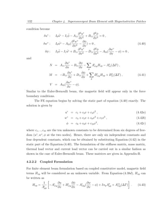
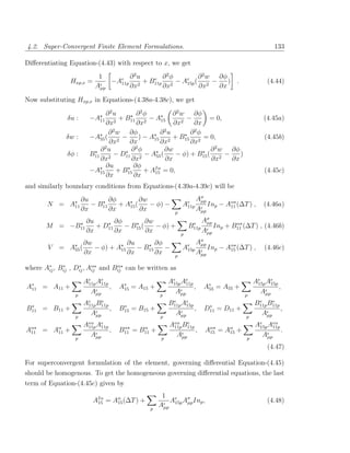
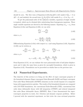
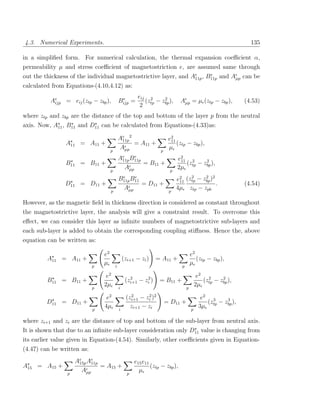
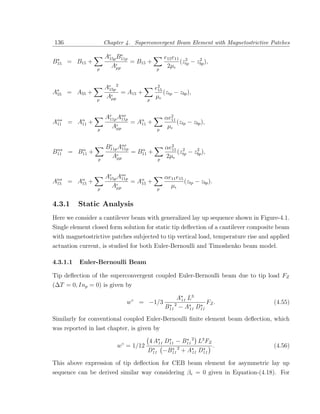
165. 4.3. Numerical Experiments. 137
50 mm
500 mm
0 0 m m
0 0 0 0
0 0 0 0
0 0 0 0
0 0 0 0
0 90 0 90
0 90 0 90
0 90 0 90
0 90 0 90
0 90 m m
[0 ] [0 /90 ] [m/0 /m] [m/0 /90 /m]
10 5 5 8 4 4
Figure 4.1: 10 layer composite cantilever beam with different layup sequence
B11 = 0, both the results are same. The ratio of tip deflections of the superconvergent
solution of the present element and the conventional element due to tip vertical load is
given by
4A11 D11
. (4.57)
4A11 D11 − B11 2
Next we will consider a case, where we have both coil current (Inp ) and temperature rise
(∆T ) (with out any tip load, FZ = 0). Tip deflections for both the formulations are same
for current and temperature load. The tip deflections due to both superconvergent and

166. 138 Chapter 4. Superconvergent Beam Element with Magnetostrictive Patches
conventional formulations are given by
 
 ◦   − L − D11 Ae r + B11 B11p r e

 u  
 11p 

◦ 1 2 e e
w = −1/2 L − B11 A11p r + A11 B11p r Inp
  (B11 2 − A11 D11 ) p  

φ  − L − B Ae r + A B e r 
11 11p 11 11p
   
α
 −B11 LB11   D11 LA11 α 
   
1    
+  −1/2 L2 Aα B11 + 2 α
1/2 L A11 B11  (∆T ). (4.58)
(B11 2 − A11 D11 )  
11
  
  
 −LAα B   LA B α 
11 11 11 11
Ratio between tip deflection and tip slope for temperature rise or actuation current is
given by
w◦ L
=
φ 2
α
One interesting observation is if A11 B11 = B11 Aα , irrespective of the thermal coefficient
11
distribution along the depth, beam will remain straight under temperature rise. Similar
e
effect will happen for actuation current if A11 B11p = B11 Ae .
11p
4.3.1.2 Timoshenko Beam
Tip deflection of the superconvergent coupled Timoshenko beam due to tip load FZ is
given by
◦ A11 D11 − 3A11 L2 ψA55 − B11 2 LFZ
w = , (4.59)
6A55 (14ψ − 1)(A11 D11 − B11 2 ) + A11 L2 ψA55
where ψ = 1/(12 + L2 βf ). Similarly, the deflection at the tip of the single element
cantilever beam for conventional (RIFSDT) element with linear shape function is given
by
A11 A55 L2 + 3A11 D11 − 3B11 2 L
w◦ = 4 FZ . (4.60)
A55 −12B11 2 + A11 A55 L2 + 12A11 D11
Tip deflection due to applied current and temperature rise in ScFSDT beam is given
by
Lr (1 − 14ψ)(B11 B11p − D11 Ae ) + L2 ψA55 Ae
e
11p 11p
u◦ = − Inp
p
(14ψ − 1)(A11 D11 − B11 2 ) + A11 L2 ψA55
L {(1 − 14ψ)(B11 B11 − D11 Aα ) + L2 ψA55 Aα }
α
11 11
− 2 2 ψA
(∆T ),
(14ψ − 1)(A11 D11 − B11 ) + A11 L 55

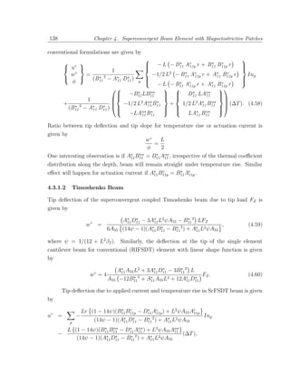
167. 4.3. Numerical Experiments. 139
L2 r(1 − 21ψ)(B11 Ae − A11 B11p )
11p
e
w◦ = Inp
p
3 (14ψ − 1)(A11 D11 − B11 2 ) + A11 L2 ψA55
L2 (1 − 21ψ)(B11 Aα − A11 B11 )
11
α
+ (∆T ),
3 (14ψ − 1)(A11 D11 − B11 2 ) + A11 L2 ψA55
Lr(1 − 14ψ)(B11 Ae − A11 B11p )
11p
e
φ = Inp
p
(14ψ − 1)(A11 D11 − B11 2 ) + A11 L2 ψA55
L(1 − 14ψ)(B11 Aα − A11 B11 )
11
α
+ (∆T ).
(14ψ − 1)(A11 D11 − B11 2 ) + A11 L2 ψA55
Ratio between tip deflection and tip slope for temperature rise or actuation current is
given by
w◦ L(1 − 21ψ)
=
φ 3(1 − 14ψ)
α
Similar to Euler-Bernoulli formulation, if A11 B11 = B11 Aα , irrespective of the thermal
11
coefficient distribution along the depth, beam will remain straight under temperature rise.
e
This effect will also be observed for actuation current, if A11 B11p = B11 Ae .
11p
4.3.1.3 Single Element Performance for Static Analysis
In this section, single element solution of static tip deflection and first three natural fre-
quencies are obtained for a 500 mm long 50 mm thick cantilever composite beam with
different lay up sequences (which is shown in Figure-4.1). Elastic modulus of composite
is taken as 181 GPa and 10.3 GPa in parallel and perpendicular direction of the fiber.
Poisson’s ratio, density and shear modulus of composite is assumed as 0.0, 1600 kg/m3
and 28 GPa respectively. Elastic modulus, Poisson’s ratio, shear modulus and density
of the magnetostrictive material is assumed as 30 GPa, 0.0, 23 GPa and 9250 kg/m3 re-
spectively. Magneto-mechanical coupling coefficient is taken as 15X10−9 m/amp. Results
are compared with 2-D plane strain finite element solution taking 100X10, four noded
quadratic elements. Single element RIFSDT results are also compared with the super
convergent and 2-D FEM results. Static tip deflections are calculated for tip vertical load
of 1 kN. Table-(4.1) shows the tip deflection for tip vertical load of [010 ] and [05 /905 ] lay
up sequence. For symmetric layup sequence ([010 ]), formulation of ScEB and CEB are
same hence their results are within 1.8% error. Here CFSDT, which is first order shear
deformable element with full integration, is giving absurd result of 94% error. RIFSDT
is showing 24.7% error and ScFSDT is within 0.2% error. Similarly for asymmetric layup

168. 140 Chapter 4. Superconvergent Beam Element with Magnetostrictive Patches
Table 4.1: Tip Deflection (mm) for Static Tip Load of 1 kN
[010 ] [05 /905 ]
CEB 0.442 (1.8 %) 1.766 (15.3 %)
ScEB 0.442 (1.8 %) 2.076 (0.5%)
CFSDT 0.027 (94 %) 0.028 (98.7%)
ScFSDT 0.449 (0.2 %) 2.083 (0.1%)
RIFSDT 0.339 (24.7 %) 1.564 (25%)
2D FEM 0.450 (0 %) 2.086 (0 %)
sequence ([05 /905 ]), CFSDT is giving an error of 98%. RIFSDT is showing 25% error
and ScFSDT is within 0.2% error. Table-(4.2) shows the tip deflection for [m/08 /m] and
Table 4.2: Tip Deflection (mm) for Static Tip Load of 1 kN
[m/08 /m] [m/04 /904 /m]
CEB uncoupled 0.746 (1.3%) 1.959 (11%)
ScEB uncoupled 0.746 (1.3%) 2.192 (0.4%)
CFSDT uncoupled 0.029 (96%) 0.293 (86.7%)
ScFSDT uncoupled 0.753 (0.4%) 2.200 (0.05%)
RIFSDT uncoupled 0.567 (25 %) 1.652 (25%)
2D FEM uncoupled 0.756 (0 %) 2.201 (0%)
CEB coupled 0.644 (1.3%) 1.327 (8.3%)
ScEB coupled 0.644 (1.3%) 1.439 (0.6%)
CFSDT coupled 0.029 (95.6%) 0.292 (80%)
ScFSDT coupled 0.651 (0.3%) 1.446 (0.07%)
RIFSDT coupled 0.490 (25%) 1.088 (24.8%)
2D FEM coupled 0.653 (0%) 1.447 (0%)
[m/04 /904 /m] lay up sequence for both coupled and uncoupled formulation. Here for both
coupled and uncoupled ScFSDT formulation, error in tip deflection is within 0.5 and 0.1%
in [m/08 /m] and [m/04 /904 /m] layup sequence respectively. For uncoupled formulation
([m/04 /904 /m]) CEB is giving 11% error. These errors for ScEB formulation are 1.3 and
0.6%. Super convergent formulation is giving less than 2.0% error, RIFSDT is giving 25%
error and CFSDT is above 80% error. Table-(4.3) shows the tip deflection for tip vertical
load for a beam with [m/08 /m] and [m/04 /904 /m] lay up sequence for both coupled and
uncoupled analysis. Static tip deflections are calculated for coil current of 1.0 ampere
with 20000 turn/m coil turns. As the difference between conventional and ScEB beam is
on vertical deflection for vertical load, results are same for actuation current, which gives
axial load and moment. Again, conventional FSDT gives absurd result.

169. 4.3. Numerical Experiments. 141
Table 4.3: Tip Deflection (mm) for Actuation Current
[m/08 /m] [m/04 /904 /m]
CEB uncoupled 0.1132 0.2105
ScEB uncoupled 0.1132 0.2105
CFSDT uncoupled 0.0043 0.0028
ScFSDT uncoupled 0.1132 0.2105
RIFSDT uncoupled 0.1132 0.2105
2D FEM uncoupled 0.1131 0.2106
CEB coupled 0.2112 0.3120
ScEB coupled 0.2112 0.3120
CFSDT coupled 0.0093 0.0063
ScFSDT coupled 0.2112 0.3120
RIFSDT coupled 0.2112 0.3124
2D FEM coupled 0.2109 0.3115
The results are showing that single super convergent element for both ScEB and
ScFSDT assumption is sufficient to get the tip deflection of the beam for tip vertical load
with in 2.0% error. Single element CFSDT is giving absurd result (error of 94-95%) due
to linear shape function use in element formulation even for thick beam. As the Euler
Bernoulli (EB) assumption is stiffer than FSDT assumption, error in ScEB formulation
(1.8%) is more than ScFSDT formulation (0.5%) and this difference is more for thicker
beams.
4.3.2 Free Vibration Analysis.
4.3.2.1 Single Element Analysis.
Table-(4.4) shows the natural frequencies for [010 ] and [05 /905 ] lay up sequence. First nat-
ural frequency for all the formulations is reasonable except for the conventional FSDT.
Second and third natural frequencies of the beam are best for ScFSDT and ScEB formu-
lations. Table-(4.5) shows the natural frequencies for [m/08 /m] and [m/04 /904 /m] lay
up sequence for both coupled and uncoupled analysis. First natural frequency for all the
formulations is reasonable except for the conventional FSDT. Second and third natural
frequencies are best for ScFSDT and ScEB formulations, when compared to 2-D FEM
results.

170. 142 Chapter 4. Superconvergent Beam Element with Magnetostrictive Patches
Table 4.4: First Three Natural Frequencies (Hz)
[010 ] [05 /905 ]
CEB 344 3321 5864 180 2033 4460
ScEB 344 3321 5864 159 1510 4302
CFSDT 1179 5864 46541 1157 4254 46367
ScFSDT 341 3241 5864 158 1502 4303
RIFSDT 334 5864 3E18 155 4253 40237
2D FEM 338 1940 4865 157 948 2505
Table 4.5: First Three Natural Frequencies (Hz)
[m/08 /m] [m/04 /904 /m]
CEB uncoupled 189 1799 3827 121 1240 2899
ScEB uncoupled 189 1799 3827 110 1041 2845
CFSDT uncoupled 820 3827 24972 812 2828 24923
ScFSDT uncoupled 188 1772 3827 110 1036 2845
RIFSDT uncoupled 185 3827 16E14 108 2828 21631
2D FEM uncoupled 187 1087 2758 110 659 1740
CEB coupled 204 1937 3914 145 1435 3011
ScEB coupled 204 1937 3914 136 1286 2961
CFSDT coupled 822 3914 24991 814 2945 24942
ScFSDT coupled 202 1903 3914 136 1276 2962
RIFSDT coupled 298 3914 53E5 133 2945 21654
2D FEM coupled 200 1116 2940 135 808 2116
4.3.3 Super convergence Study.
4.3.3.1 Free Vibration Analysis.
Figure-4.2 shows the percentage errors of the first 10 natural frequencies of [010 ] layup
sequence. Here we have compared the natural frequencies for RIFSDT, ScFSDT, CEB
(CEB and ScEB are same for symmetric layup sequence), FSDT Full (CFSDT) and 2-D
FEM formulation. For first seven natural frequencies, 10 ScFSDT elements give better
result than 20 RIFSDT elements. This shows the super convergence properties of the
ScFSDT elements. The 8th , 9th and 10th natural frequencies for 20 elements RIFSDT
gives little better result than 10 elements ScFSDT. Figure-4.3 shows the percentage errors
of the first 10 natural frequencies of [05 /905 ] layup sequence. Here all first 10 natural
frequencies 10 ScFSDT elements give better result than 20 RIFSDT elements. Similarly
10 ScEB elements give better result than 20 CEB elements. This shows that asymmetric
layup sequence exhibit a greater level of super convergence property. 20 elements FSDT

171. 4.3. Numerical Experiments. 143
25
500X10 2D−FEM
20 RIFSDT
10 CEB
10 ScFSDT
20
10 FSDT Full
Natural Frequency Error (%)
15
10
5
0
1 2 3 4 5 6 7 8 9 10
Frequency Number
Figure 4.2: Natural Frequency for Cantilever Beam with [010 ] Layup sequence
25
500X10 2D−FEM
20 RIFSDT
10 ScEB
20 CEB
20
10 ScFSDT
Natural Frequency Error (%)
20 CFSDT
15
10
5
0
1 2 3 4 5 6 7 8 9 10
Frequency
Figure 4.3: Natural Frequency for Cantilever Beam with [05 /905 ] Layup sequence

172. 144 Chapter 4. Superconvergent Beam Element with Magnetostrictive Patches
60
500X10 2D−FEM
20 RIFSDT
10 ScEB
50 10 ScFSDT
20 CFSDT
Natural Frequency Error (%)
40
30
20
10
0
1 2 3 4 5 6 7 8 9 10
Frequency Number
Figure 4.4: Natural Frequency for Beam with Coupled, [m/08 /m] Layup sequence
60
500X10 2D−FEM
20 RIFSDT
10 ScEB
50 10 ScFSDT
20 CFSDT
Natural Frequency Error (%)
40
30
20
10
0
1 2 3 4 5 6 7 8 9 10
Frequency Number
Figure 4.5: Natural Frequency for Beam with Uncoupled, [m/08 /m] Layup sequence

173. 4.3. Numerical Experiments. 145
25
500X10 2D−FEM
20 RIFSDT
10 ScEB
20 CEB
20
10 ScFSDT
Natural Frequency Error (%)
20 CFSDT
15
10
5
0
1 2 3 4 5 6 7 8 9 10
Frequency
Figure 4.6: Natural Frequency for Beam with Coupled, [m/04 /904 /m] Layup sequence
25
500X10 2D−FEM
20 RIFSDT
10 ScEB
20 CEB
20
10 ScFSDT
Natural Frequency Error (%)
20 CFSDT
15
10
5
0
1 2 3 4 5 6 7 8 9 10
Frequency
Figure 4.7: Natural Frequency for Beam with Uncoupled, [m/04 /904 /m] Layup sequence

174. 146 Chapter 4. Superconvergent Beam Element with Magnetostrictive Patches
Full (CFSDT) gives worst result for this asymmetric layup sequence.
Figure-4.4 and Figure-4.5 show the percentage errors of the first 10 natural frequencies of
coupled and uncoupled material model for [m/08 /m] layup sequence. In this symmetric
layup sequence, first 8 natural frequencies with 10 ScFSDT elements give better result
than 20 RIFSDT elements. The 9th and 10th natural frequencies for 20 elements RIFSDT
give little better result than 10 elements ScFSDT.
Figure-4.6 and Figure-4.7 show the percentage errors of the first 10 natural frequencies
of coupled and uncoupled material model for [m/04 /904 /m] layup sequence. In coupled
formulation, first 9 natural frequencies for 10 ScFSDT elements show better result than 20
RIFSDT elements. Similarly 10 ScEB elements give better result than 20 CEB elements.
In uncoupled formulation (where asymmetry is more than in the coupled formulation),
for first 10 natural frequencies (except 8th ) using 10 ScFSDT elements give better result
than 20 RIFSDT elements. Again results from 20 CEB elements are comparable with
10 ScEB elements. Twenty elements of FSDT Full (CFSDT) give worst result for this
asymmetric layup sequence. This study to a reasonable extent has shown the super-
convergent character of the formulated elements. This can be further studied using the
time history analysis, which is given next.
4.3.3.2 Time History Analysis.
Vertical impact load shown in Figure-4.8 is applied at the cantilever tip. Tip response and
the open circuit voltage in the sensor coil are obtained for different number of elements for
this impact loading. Figure-4.9 shows the effect of beam assumption on tip velocity of the
cantilever beam taking 100 elements of ScEB and ScFSDT and the results are compared
with 2-D FEM, which is modelled with 1000 2D four noded plane stress element. Two
aspects are very clear from this study. A 100 element ScFSDT model compares very
well with 2D FEM solution and the waves in shear deformable beams travel much slower
compared to elementary beam. This can be seen as early arrival of reflection in ScEB
model. Figure-4.10(a) shows the super convergent properties of the ScFSDT element for
a unidirectional laminate. Here 10 ScFSDT element model is giving similar result as 20
RIFSDT elements and these match well with 2D FEM solution.
Figure-4.10(b) shows the tip velocity history for [05 /905 ] layup sequence. Here 10 of
ScFSDT elements are giving better result than 20 RIFSDT elements. Figure-4.11 shows
the open circuit voltages generated in a laminate of [m/08 /m] layup sequence due to tip
vertical impact. Here 10 ScFSDT elements are giving better result than 20 RIFSDT ele-

175. 4.3. Numerical Experiments. 147
0.9 −5
x 10
2.5
0.8
2
0.7
Frequency Content
0.6 1.5
Force (kN)
0.5
1
0.4
0.5
0.3
0
0.2 0 50 100
Frequency (kHz)
0.1
0
0 100 200 300 400 500 600
Time (µ sec)
Figure 4.8: 50 kHz Broadband Force History with Frequency Content (inset)
−5
x 10
12
10
8
6
Velocity (m/Sec)
4
2
0
−2
−4
−6
100 Elements ScEB
−8 100 Elements ScFSDT
100X10 Elements 2D−FEM
0 1 2 3 4 5
Time (Sec) −4
x 10
Figure 4.9: Effect of Beam Assumption on Tip Response [010 ]

176. 148 Chapter 4. Superconvergent Beam Element with Magnetostrictive Patches
−5
x 10
12
10
8
6
Velocity (m/Sec)
4
2
0
−2
−4
10 Elements RIFSDT
−6 20 Elements RIFSDT
10 Elements ScFSDT
−8 100X10 Elements 2D−FEM
0 1 2 3 4 5
Time (Sec) x 10
−4
(a) 010 layup sequence
−4
x 10
2
1.5
1
Velocity (m/Sec)
0.5
0
−0.5
10 Elements RIFSDT
20 Elements RIFSDT
10 Elements ScFSDT
−1
100X10 Elements 2D−FEM
0 1 2 3 4 5 6
Time (Sec) x 10
−4
(b) 05 /905 Layup sequence
Figure 4.10: Superconvergent Study of ScFSDT elements

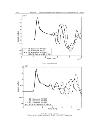
177. 4.3. Numerical Experiments. 149
0.15
0.1
Open Circuit Voltage (volt)
0.05
0
−0.05
−0.1 10 Elements RIFSDT
20 Elements RIFSDT
10 Elements ScFSDT
−0.15 100X10 Elements 2D−FEM
0 1 2 3 4 5 6
Time (Sec) x 10
−4
Figure 4.11: Open circuit voltage for Coupled, [m/08 /s] Layup sequence
ments. These studies have shown that the formulated element is indeed superconvergent
and can find great utilities in the SHM application. In the next section, we will use this
formulated element to perform an inverse problem of material property identification us-
ing the measured response. In this problem, very high degrees of intensive computations
are required and the superconvergent property of the formulated element can reduce the
problem size considerably.
4.3.4 Material Property Identification
The objective of this subsection is to identify the modulus of elasticity and magnetome-
chanical coefficient of magnetostrictive patches from the response of sensor using super
convergent elements and Artificial Neural Network (ANN). First, the sensor response is
computed for varying modulus of elasticity for a particular value of magnetomechanical

178. 150 Chapter 4. Superconvergent Beam Element with Magnetostrictive Patches
coefficient and shown that the modulus of elasticity can be identified with a polynomial
relationship from peak value of the sensor response. Similarly, in the next study, varying
values of magnetomechanical coefficient with fixed value of elastic modulus is used for
identification of magnetomechanical coefficient, which also gives a simplified polynomial
relationship to identify the magnetomechanical coefficient from peak value of the sensor
response. Finally studies are also performed for cases when both the values are vary-
ing. Due to the complexity of the problem ANN is used for identification of both elastic
modulus and magnetomechanical coefficient.
4.3.4.1 Elastic Modulus Identification
Figure-4.12 shows the sensor response of [m/04 /904 /s] layup sequence due to impact
load (shown in Figure-4.8) at the tip of the cantilever, where s stands for sensor layer.
Considering magnetomechanical coefficient as 15 nano-m/amp and three different values
of modulus, three different responses are obtained. Initial peak amplitudes for 25, 30 and
35 GPa module are 323, 468 and 736 mili-volt respectively. The initial peak values (Vp )
of these open circuit voltage histories are increased for increased values of modulus of
elasticity. One direct polynomial can be used to identify the modulus of elasticity from
these peak values or vice versa. From these three sample points, one quadratic polynomial
is drawn and elastic modulus (E) or initial peak value (Vp ) is expressed as:
Vp = 2.462X10−3 E 2 − 0.10642E + 1.4447,
E = −38.341Vp 2 + 64.822Vp + 8.0588. (4.61)
Now these results are validated for two other values of modulus, namely 27 and 32 GPa,
respectively. Initial peak values of voltage histories for corresponding module are 372
and 554 mili-volt respectively from finite element analysis. And the predicted elastic
moduli from this polynomial are 26.88 and 32.19 GPa respectively, which are with in 1%
of accuracy.
4.3.4.2 Magnetomechanical Coefficient Identification
Figure-4.13 shows the sensor response of the [m/04 /904 /s] layup sequence due to impact
load (shown in Figure-4.8) at the tip of the cantilever. Considering magnetomechanical
coefficient as 5, 10 and 15 nano-m/amp and with a fixed value of modulus as 30 GPa,
three different curves are obtained. The initial peak values of open circuit voltages are
increased for increased values of magnetomechanical coefficient. One direct polynomial

179. 4.3. Numerical Experiments. 151
0.8
0.6
Open Circuit Voltages (volt)
0.4
0.2
0
−0.2
−0.4 E=25 GPa
E=30 GPa
E=35 GPa
0 1 2 3 4 5 6
Time (sec) x 10
−4
Figure 4.12: Sensor voltage for coupled, [m/04 /904 /s] with varying elasticity
0.4
0.3
Open Circuit Voltages (volt)
0.2
0.1
0
−0.1
−0.2
−0.3
d=5 nano−m/amp
−0.4 d=10 nano−m/amp
d=15 nano−m/amp
0 1 2 3 4 5 6
Time (sec) x 10
−4
Figure 4.13: Sensor voltage for Coupled, [m/04 /904 /s] with varying coupling coefficient

180. 152 Chapter 4. Superconvergent Beam Element with Magnetostrictive Patches
is used to identify the magnetomechanical coefficient from this peak value or vice versa.
From these three sample points two quadratic polynomials are drawn as:
Vp = 3.9878X1015 d2 − 3.9603X107 d + 0.16486,
d = −8.1759X10−8 Vp 2 + 6.8613X10−8 Vp + 7.967. (4.62)
For validation of these curves, two other values of coupling coefficient, namely, 7 and 12
nano-m/amp are used in simulation. Initial peak values considering corresponding coeffi-
cients are 99 and 238 mili-volt respectively from finite element analysis. And the predicted
coupling coefficients from above polynomial are 6.8 and 12.5 nano-m/amp respectively,
which are with in 4% of accuracy.
4.3.4.3 Material Properties Identification using ANN
0.15
Open Circuit Voltages (volt)
0.1
0.05
0
−0.05
d=5 nano−m/amp; E=25 GPa
−0.1 d=5 nano−m/amp; E=35 GPa
d=10 nano−m/amp; E=25 GPa
d=10 nano−m/amp; E=35 GPa
0 1 2 3 4 5 6
Time (sec) x 10
−4
Figure 4.14: Open circuit voltage for Coupled, [m/04 /904 /s] layup sequence

181. 4.3. Numerical Experiments. 153
In the above discussion, either coupling coefficient is identified assuming elastic
modulus of magnetostrictive materials or modulus of elasticity is identified assuming
magnetomechanical coupling coefficient. But in real time structural health monitoring
application both the values should be identified simultaneously using measured sensor
responses. Figure-4.14 shows the sensor response of the [m/04 /904 /s] layup sequence due
to impact load shown in Figure-4.8 considering both magnetomechanical coefficient and
modulus of elasticity as varying. The initial peak value of open circuit voltages are in-
creased due to increase of both these values as shown in earlier two figures. Hence, it is not
possible to identify both the properties from initial peak values of open circuit voltages.
Hence, utilization of the rest of the response histories is essential in this identification,
which can be performed using Artificial Neural Network (ANN) easily.
The main goal of this subsection is to establish a mapping relation from sensor
response histories to the material properties. ANN is trained and validated for this map-
ping. Training of ANN is performed through 121 sample response histories, which are
consist of 11 values of elastic modulus (from 25 to 35 GPa with increment of 1 GPa)
each for 11 values of magnetomechanical coupling coefficients (from 5 to 15 nano-m/amp
with increment of 1 nano-m/amp). Every simulation takes about 30 seconds in Pentium-4
processor with the use of 20 ScFSDT elements. Hence, total time required for simulation
of training samples is about one hour. On the other hand, every simulation using 50
RIFSDT elements takes one minute, and hence about 2 hours are required for all sam-
ples. Response histories are captured upto 600 time steps. Hence, if raw responses are
directly fed into ANN as input, input space of the ANN architecture will be 600, which
will be difficult to manage. Hence, some specific peak values and their corresponding
location of response histories is considered for input space of the ANN. Whole response
histories are divided into three parts. First part is from 0 to 200 µ sec, middle part is
from 200 to 400 µ sec, and last part is from 400 to 600 µ sec. In the first part only
peak value of response histories (shown in Table-4.6) is taken as first input node for the
ANN mapping. Location of the first peak value are not considered as input node of ANN,
since the sensitivity of that location regarding elastic modulus or magnetomechanical co-
efficient is less. From middle and last part of the response histories peak values (shown
in Table-4.7, 4.9) and peak locations (shown in Table-4.8, 4.10) are taken as other four
input nodes. Total five input nodes are considered as input space of ANN mapping. Two
output nodes are considered, one for elastic modulus and other for magnetomechanical
coefficient as output space of the ANN mapping. To determine the architecture of the

182. 154 Chapter 4. Superconvergent Beam Element with Magnetostrictive Patches
Table 4.6: First peak amplitude of training samples (mili-volt)
25 26 27 28 29 30 31 32 33 34 35
5 57 59 61 63 65 67 69 71 73 74 76
6 71 73 75 78 80 83 85 88 90 92 95
7 85 88 91 94 97 100 103 106 109 112 115
8 101 104 108 112 116 120 124 127 131 139 139
9 118 123 128 132 137 142 147 152 156 166 161
10 138 144 150 156 162 168 174 180 187 193 199
11 162 169 177 184 192 199 207 215 224 232 241
12 190 199 208 218 228 238 249 260 271 283 295
13 224 236 248 261 275 289 304 320 337 354 373
14 267 283 300 319 338 360 383 408 435 465 498
15 324 347 373 401 433 469 509 554 605 665 737
Table 4.7: Middle peak amplitude of training samples (mili-volt)
25 26 27 28 29 30 31 32 33 34 35
5 11 12 12 12 13 13 13 14 14 14 15
6 14 14 15 15 15 16 16 17 17 18 18
7 16 17 17 18 18 19 20 20 21 21 22
8 19 20 20 21 22 22 23 24 25 27 27
9 22 23 24 25 26 27 28 29 30 32 31
10 26 27 28 29 30 32 33 34 35 37 38
11 30 31 33 34 36 37 39 41 42 44 46
12 35 37 39 41 43 45 47 50 52 55 58
13 41 43 46 49 52 55 59 63 67 71 76
14 49 52 56 61 66 71 77 84 92 99 105
15 61 67 73 80 89 99 108 116 120 121 131
Table 4.8: Middle peak location of training samples (micro-second)
25 26 27 28 29 30 31 32 33 34 35
5 321 320 319 319 318 318 317 317 316 316 316
6 320 320 319 318 318 317 317 316 316 316 315
7 320 319 318 318 317 317 316 316 316 315 315
8 319 318 318 317 317 316 316 315 315 314 314
9 318 318 317 316 316 316 315 314 314 312 313
10 318 317 316 316 315 315 314 313 312 311 311
11 317 316 316 315 314 313 312 311 310 309 308
12 316 315 314 313 312 311 310 308 307 305 303
13 314 313 312 311 309 307 305 304 302 300 298
14 312 310 309 306 304 302 300 298 295 292 289
15 308 306 303 301 298 295 291 287 282 276 268

183. 4.3. Numerical Experiments. 155
Table 4.9: Last peak amplitude of training samples (mili-volt)
25 26 27 28 29 30 31 32 33 34 35
5 43 44 44 44 44 43 42 42 42 42 42
6 52 53 53 52 52 51 50 50 51 52 53
7 61 62 61 60 59 59 59 60 61 63 64
8 70 70 69 68 67 68 69 71 73 76 76
9 79 77 77 77 78 80 82 84 86 89 87
10 86 86 87 89 91 93 95 96 99 102 108
11 95 97 99 101 103 105 108 114 123 132 141
12 108 110 111 113 118 127 139 151 160 166 171
13 119 120 127 141 156 169 178 184 189 195 201
14 136 153 171 185 194 200 208 217 220 214 202
15 184 199 207 218 230 233 223 209 216 234 234
Table 4.10: Last peak location of training samples (micro-second)
25 26 27 28 29 30 31 32 33 34 35
5 545 542 539 535 532 529 526 522 518 515 511
6 543 539 536 533 529 526 521 517 514 511 507
7 540 536 533 529 525 520 516 512 509 507 502
8 536 532 528 524 519 514 511 507 503 498 498
9 532 527 522 517 512 508 504 500 498 489 493
10 526 520 515 511 505 502 498 493 488 484 479
11 518 512 507 502 498 493 487 482 477 472 468
12 511 504 499 493 486 480 475 470 465 460 456
13 500 493 486 479 473 467 462 456 450 444 439
14 487 479 472 465 459 452 444 438 431 425 417
15 472 464 456 447 439 431 423 414 404 396 389
ANN, four different ANN (5-2-2;5-3-2;5-4-2;5-5-2) are considered with the above men-
tioned training samples. Training histories of these networks are shown in Figure-4.15.
Figure shows, ANN architecture (5-4-2) with four hidden layer nodes (Figure-4.16(c))
gives better training performance, and this architecture is considered for the subsequent
studies. Figure-4.16(c) shows the ANN architecture with 5 input nodes, 2 output nodes
and one hidden layer with 4 hidden nodes. Two output nodes are for modulus of elasticity
and coupling coefficient, where as input nodes, which are five in number corresponding to
the five values obtained from response histories as discussed earlier. After the training of
the ANN using training samples, these same samples are simulated in the trained ANN to
check the training performance of the ANN. Figure-4.17 shows the training performance
of this ANN after 10000 epoch of training. Expected and predicted location in the output

184. 156 Chapter 4. Superconvergent Beam Element with Magnetostrictive Patches
Net Arch 5−2−2
Net Arch 5−3−2
2 Net Arch 5−4−2
10 Net Arch 5−5−2
Mean Square Error
1
10
0
10
−1
10
0 1 2 3
10 10 10 10
Epoch
Figure 4.15: Training Histories of different ANN architectures
space of the training samples are shown as ∗ and ◦ respectively. After checking the
training performance for generalization of the mapping, networks are validated with a
different set of samples, which are not been used for training purpose in the network.
For validation, 100 intermediate sample response histories are obtained in finite element
simulation, which are for 10 values of elastic modulus (from 25.5 to 34.5 GPa with in-
crement of 1 GPa) each for 10 values of magnetomechanical coupling coefficients (from
5.5 to 14.5 nano-m/amp with increment of 1 nano-m/amp). Similar to training phase,
five input nodes of ANN mapping are extracted from these response histories and given
in Tables-4.11, 4.12, 4.13, 4.14, and 4.15, respectively. Finally, these validation samples
are used to simulate in ANN and corresponding prediction for both elastic modulus and
magnetomechanical coupling coefficient are obtained. Figure-4.18 shows the validation
performance of the network, where expected and predicted location in the output space

185. 4.3. Numerical Experiments. 157
Table 4.11: First peak amplitude of validation samples (mili-volt)
25.5 26.5 27.5 28.5 29.5 30.5 31.5 32.5 33.5 34.5
5.5 64 66 68 71 73 75 77 79 81 83
6.5 78 81 83 86 89 92 94 97 100 102
7.5 93 97 100 104 107 110 114 117 120 124
8.5 110 115 119 123 127 132 136 140 144 149
9.5 130 135 140 145 151 156 162 167 173 178
10.5 152 158 165 172 179 185 192 199 207 214
11.5 178 186 195 204 212 221 230 240 250 260
12.5 210 221 232 243 255 267 280 293 307 322
13.5 250 264 279 295 311 329 348 368 390 414
14.5 301 321 343 367 392 421 452 487 526 569
Table 4.12: Middle peak amplitude of validation samples (mili-volt)
25.5 26.5 27.5 28.5 29.5 30.5 31.5 32.5 33.5 34.5
5.5 12 12 12 13 13 14 14 14 15 15
6.5 14 15 15 16 16 17 17 18 18 19
7.5 17 18 18 19 19 20 21 21 22 23
8.5 20 21 21 22 23 24 25 26 27 27
9.5 23 24 25 26 27 28 30 31 32 33
10.5 27 28 30 31 33 34 35 37 38 40
11.5 32 33 35 37 39 41 43 45 47 49
12.5 38 40 42 44 47 50 53 56 60 63
13.5 45 48 51 55 59 64 68 73 79 86
14.5 55 60 66 72 78 86 95 103 110 115
Table 4.13: Middle peak location of validation samples (micro-second)
25.5 26.5 27.5 28.5 29.5 30.5 31.5 32.5 33.5 34.5
5.5 320 320 319 318 318 317 317 316 316 316
6.5 320 319 318 318 317 317 316 316 316 315
7.5 319 319 318 317 317 316 316 316 315 315
8.5 319 318 317 317 316 316 315 315 314 313
9.5 318 317 317 316 316 315 314 313 313 312
10.5 317 316 316 315 314 313 312 312 311 310
11.5 316 315 314 313 312 311 310 309 308 307
12.5 315 313 312 311 310 309 307 305 303 302
13.5 312 311 310 308 306 304 302 300 298 296
14.5 310 307 305 302 300 298 295 292 288 284

186. 158 Chapter 4. Superconvergent Beam Element with Magnetostrictive Patches
Output
Output
Input
Input
Hidden Layer
Output Layer Hidden Layer Output Layer
Input Layer Input Layer
(a) 5-2-2 architectures (b) 5-3-2 architectures
Output
Output
Input
Input
Output Layer Output Layer
Hidden Layer
Input Layer Input Layer Hidden Layer
(c) 5-4-2 architectures (d) 5-5-2 architectures
Figure 4.16: ANN with Different architectures
of the validation samples are shown as 2 and ’x’ respectively. Using these ANN, feed-
ing any response histories, the corresponding elastic modulus and magnetomechanical
coupling coefficient can be identified with in 1% accuracy.

187. 4.3. Numerical Experiments. 159
35
34
33
Modulus of Elasticity (GPa)
32
31
30
29
28
27
26
25
5 10 15
Magnetomechanical Coefficient (nano−m/amp)
Figure 4.17: Training Performance of 5-4-2 ANN architectures
35
34
33
Modulus of Elasticity (GPa)
32
31
30
29
28
27
26
25
5 10 15
Magnetomechanical Coefficient (nano−m/amp)
Figure 4.18: Validation Performance of 5-4-2 ANN architectures

188. 160 Chapter 4. Superconvergent Beam Element with Magnetostrictive Patches
Table 4.14: Last peak amplitude of validation samples (mili-volt)
25.5 26.5 27.5 28.5 29.5 30.5 31.5 32.5 33.5 34.5
5.5 47 47 48 47 46 46 45 45 45 46
6.5 56 56 56 55 54 53 53 54 55 57
7.5 65 65 64 62 62 62 64 65 67 68
8.5 73 72 71 71 72 74 76 78 79 81
9.5 81 80 81 82 84 86 88 90 92 94
10.5 90 91 93 95 97 98 101 104 110 118
11.5 102 104 105 107 110 115 124 135 145 153
12.5 113 114 118 127 140 153 164 171 176 180
13.5 126 137 154 170 181 188 193 201 208 212
14.5 167 184 195 203 213 223 226 217 203 508
Table 4.15: Last peak location of validation samples (micro-second)
25.5 26.5 27.5 28.5 29.5 30.5 31.5 32.5 33.5 34.5
5.5 542 539 536 533 529 526 522 518 514 510
6.5 540 536 533 529 525 521 517 513 510 506
7.5 536 533 529 524 520 515 510 508 505 501
8.5 532 528 523 518 514 509 506 501 499 495
9.5 526 521 516 510 506 503 499 495 491 487
10.5 519 514 509 504 500 495 490 485 480 476
11.5 510 506 501 495 490 484 478 473 469 465
12.5 501 496 490 483 477 471 466 461 456 450
13.5 490 483 476 469 463 457 451 444 438 432
14.5 476 469 461 454 446 438 431 424 415 468
4.4 Summary
This study is mainly intended to explore the use of superconvergent FE formulation
for the analysis of smart composite structures with magnetostrictive patches and their
utility in solving inverse problems. Classical and shear deformable beam elements for the
analysis of composite beam with embedded magnetostrictive patches are formulated. The
consistent mass matrix is derived using the exact solution to the static part of governing
equation. Rotary inertia is also taken into account. The formulated element is then used
to study the superconvergent property in static, free vibration, and wave propagation
problems in composite beams embedded with magnetostrictive patches. The effect of
superconvergence was shown in all these problems. The formulated element was later
used for identification of the magnetostrictive material properties using using artificial
neural network, where superconvergent elements are utilized to get sensor response in

189. 4.4. Summary 161
finite element simulation with lesser computation time, where ANN is used for mapping
from sensor response to properties of the magnetostrictive materials. In the next chapter,
we will again concentrate on developing better and more accurate numerical / analytical
model for analysis of smart laminated composite structure. This model is called the
spectral finite element model.

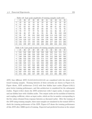
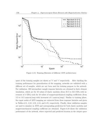
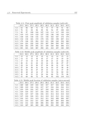
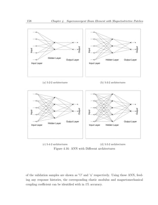
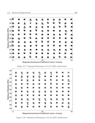
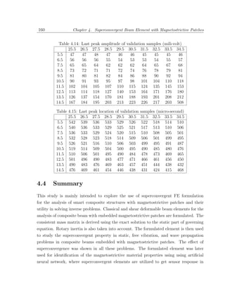
190. Chapter 5
Spectral FE Analysis with
Magnetostrictive Patches
5.1 Introduction
As mentioned earlier, determination of smaller cracks requires signals having high fre-
quency content. That is, the problem translates itself to a wave propagation problem,
wherein, in addition to phase information of the response being important, higher order
modes participate in the response. For such problem, FEM requires enormous mesh sizes.
This problem can be alleviated little using superconvergent elements. The best way to
handle such situation is to formulate elements in the frequency domain. Spectral FE is
one such formulation that will be addressed in this chapter.
Wave propagation in a structure is caused by high frequency impact loading. When
such loading is applied to a structure, it will force all the higher-order modes to participate
in the response. At high frequencies, the wavelength is small and for an accurate predic-
tion by the finite element (FE) method, the element length should be one fourth to one
sixth of the wavelength [196]. Hence, FE analysis of wave propagation incurs heavy com-
putational costs. The spectral element method (SEM) is arguably the best alternative for
such problems [108]. The method is based upon the domain transfer method. Here, the
governing equation is transformed first into the frequency domain using a discrete Fourier
transform (DFT). In doing so, for 1-D waveguides, the governing partial differential equa-
tion (PDE) is reduced to a set of ordinary differential equations (ODE) with constant
coefficients, where the time coordinate gives way to the frequency, which is introduced as
a parameter. The resulting ODEs can be solved exactly. The elements are formulated
using the exact solution of the governing ODEs as an interpolating function. The use
of the exact solution results in an exact mass distribution and thus in an exact dynamic
162

191. 5.1. Introduction 163
stiffness matrix. Hence, in absence of any discontinuity or irregularity in geometry, one
element is sufficient to handle a beam of any length. This feature substantially reduces
the size of the global dynamic stiffness matrix to be inverted and the problem (matrix)
size is many orders smaller than the sizes involved in conventional FEM. The steps to be
followed in SEM are as follows: First, the input forcing function is fed into Fast Fourier
Transform (FFT) program, which will split the forcing history into frequencies, and the
real and imaginary parts of the force history. These frequencies are real, and element
dynamic stiffness matrix is generated at each frequency. These are assembled and solved
as in conventional FEM. After assembly, the structure is solved for unit impulse; which
will directly give Frequency Response Function (FRF). The FRF is then convolved with
load to get the required response. Finally, inverse fast Fourier transform (IFFT) is used
to get the time history of the response. In addition to the smaller system sizes, there are
many advantages inherent to the SEM. These are summarized below:
1. A compact matrix formulation is available, which can accommodate any number of
nodal variables in a spectral finite element model (SFEM) and hence suitable for
automation. It is stiffness formulated. This means the process of assemblage for
complex structures is easy.
2. The mass distribution is modelled exactly and hence only one element is sufficient to
describe a whole beam without the need for subdivisions. This makes the resulting
system of dynamic equations very small and hence computationally efficient.
3. The problem to be solved is repeated many times in data-independent manner.
This inherent parallelism of the spectral approach can be utilized on multiprocessor
machines.
4. The FRF is the direct by-product of the approach.
5. Since the system transfer function is direct by product of the approach, performing
inverse problems, such as, system identification or the force identification, is also
straightforward.
6. Infinite domain can be easily modelled by just leaving out the terms containing
the reflected coefficients from the exact solution. Such a single edge non-resonant
elements are called the throw-off element. When added to the structure, it amounts
to adding maximum damping for the structure.

192. 164 Chapter 5. Spectral FE Analysis with Magnetostrictive Patches
7. The classical static stiffness matrix can be obtained from the spectral stiffness matrix
in a zero-frequency limit.
8. Responses can be viewed both in time and frequency domain in a single analysis.
The frequency domain information such as transfer functions and system functions
are generated automatically.
9. The method is easily amenable for control related problems. A novel active spectral
element (see [246]) is formulated for this purpose. This has great utility in smart
structure research for noise and vibration suppression.
10. As opposed to using modal analysis, in the SFEM is based on computation of
wavenumbers and frequency domain fields (displacements, strains, stresses etc.) i.e.
the spectral amplitudes, at each frequency sampling points in FFT. The consid-
eration of frequency bandwidth is not limited by the choice of the finite element
discretization, i.e. even a single Spectral Element can be used for a uniform beam
excited by high frequency loads. Also, the time history of the applied load can be
arbitrary.
11. Cut-off frequency is one parameter that determines the need for higher order beam
theory. In elementary beams, the cut-off frequency is at infinity i.e. shear mode
appears as evanescent mode, which never propagates. If the frequency of interest is
within the occurrence of the cut-off frequency, then the elementary beam theory is
sufficient to predict the response. In FSDT the shear mode, which is evanescent to
start with, begins to propagate beyond cut-off frequency. This aspect will be dwelt
in greater detail in this chapter.
5.1.1 Existing Literature
Spectral elements for an elementary rod [109], elementary beam [110], [111], elementary
composite beam [249], composite tube [250], and a 2-D membrane element [330] are
reported in literature.
Several higher-order spectral elements for isotropic and anisotropic one-dimensional
wave guides are available in the literature. Spectral elements are developed for the
isotropic Mindlin Herman rod [256], the isotropic Timoshenko beam [140] and the com-
posite Timoshenko beam [248].

193. 5.1. Introduction 165
Introducing Poisson’s contraction and its higher order gradients in the displacement
field give rise to additional propagating modes at high frequencies. In addition, the
longitudinal wave in the structure becomes dispersive. Conventional Higher order Shear
Deformation Theory (HSDT) allows no depth wise variation of transverse displacement.
Further, the displacement field with lateral contraction predicts nonzero normal stress,
which is altogether neglected in HSDT. Hence, for a deep beam and high frequency
loading, HSDT will not predict the accurate dynamic response of the structure. An exact
FE was developed for isotropic materials by Gopalakrishnan [139], which takes Poisson’s
contraction into account. More recently, an exact FE is developed for a composite beam
with Poisson’s contraction [64]. Extensive study on wave propagation in anisotropic and
inhomogeneous structure is done by Chakraborty in reference [59]. In this study, he has
shown that the dispersiveness of an axial mode is due to the presence of lateral contraction.
In recent study, Batra and Aimmanee [31] used finite element mixed formulation to satisfy
traction boundary conditions on the top and the bottom surfaces with higher order shear
and normal deformable plate theories.
In this chapter, a new higher order spectral element is developed for wave propaga-
tion analysis of a magnetostrictive embedded composite beam in the presence of thermal,
magnetic and mechanical loading. The element is based on the coupled formulation of
Higher order Shear deformation with higher order Poisson contraction Theory (HSPT).
The HSDT is enhanced through the introduction of higher number of lateral contractional
mode. Numerical examples are directed towards highlighting the effect of the requirement
of higher order theories on the structural and magnetic responses. The spectrum and the
dispersion relations are studied in detail. Response of structure for high frequency mod-
ulated pulse with different order of beam assumption is outlined and shown the error
in lower order models. Magnetostrictive sensor open circuit voltages due to broadband
force excitation are computed. Finally, as a demonstration of its capability to handle
inverse problems, applied broadband force history in a cantilever composite beam is re-
constructed from the response of magnetostrictive sensor open circuit voltage history,
using deconvolution property of the spectral formulation.
This chapter is organized as follows. First the variational formulation is illustrated
to obtain the governing differential equations of Higher order Shear deformable and Pois-
son contractible (HSPT) beam. Subsequently, we derive spectral solution for these gov-
erning equations and formulate the spectral finite element of the beam element with
embedded magnetostrictive patches. In Section-5.4, several examples are considered for

194. 166 Chapter 5. Spectral FE Analysis with Magnetostrictive Patches
the verification of the element, demonstration of the importance of higher order theo-
ries, propagation of the extra shear and contraction modes, alteration in group speed due
to the presence of higher order degrees of freedom. Finally, in Subsection-5.4.2, force
identification is demonstrated from magnetostrictive sensor response.
5.2 FE Formulation of an nth Order Shear Deformable
Beam with nth Order Poisson’s Contraction
Considering the U nth order shear deformation theory along with W nth order Poisson’s
contraction effects, the axial and the transverse displacement fields can be written as
Un Wn
i
U (x, y, z, t) = u0 (x, t) + z ui (x, t) , W (x, y, z, t) = w0 (x, t) + z i wi , (5.1)
i=1 i=1
where u0 and w0 are axial and transverse displacements in the reference plane respectively
and z is thickness coordinate measured from the reference plane. wi are the contractional
strain and their higher order in transverse direction due to the effect of the Poisson ratio.
Magnetic fields are assumed as
Hx (x, y, z, t) = Hxp (x, t), Hy (x, y, z, t) = 0, Hz (x, y, z, t) = 0 (5.2)
where Hx , Hy and Hz are the component of magnetic fields at location (x , y, z ) in X ,
Y and Z direction respectively. Hxp is X directional magnetic field at mid plane of the
magnetostrictive patch p. The magnetic field along the thickness direction within the
particular layer is assumed as constant. Using Equation-(5.1), the linear strains can be
written as
Un
εxx = u0,x + z i ui,x − α∆T,
i=1
Wn
εzz = iz (i−1) wi − α∆T,
i=1
Un Wn
(i−1)
γxz = iz ui (x, t) + w0,x + z i wi,x . (5.3)
i=1 i=1
α is coefficient of thermal expansion of the material and ∆T is the temperature
change to which the beam is subjected. The constitutive relation for material is assumed

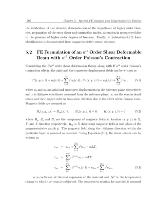
195. 5.2. FE Formulation of an nth Order Shear Deformable Beam with nth Order Poisson’s Contraction167
to be of the form
      
 σxx  ¯ ¯
Q11 Q13 0  εxx   e11 
σzz ¯ ¯
=  Q13 Q33 0  εzz − e13 H,
  ¯ 55  γxz   e15 
τxz 0 0 Q
 
 εxx 
Bxx = e11 e13 e15 εzz + µ H, (5.4)
 
γxz
where σxx and εxx , are normal stresses and normal strains in the x direction, σzz and εzz ,
are normal stresses and normal strains in the z direction and τxz and γxz are shear stress
¯ ¯ ¯ ¯
and shear strain in the x − z plane. Q11 (z), Q13 (z), Q33 (z) and Q55 (z) are Young’s and
Shear module, which are functions of depth z. The strain energy (S), magnetic energy
(Wm ) and kinetic energy (T ) are then given by
L
1
S = (σxx εxx + σzz εzz + τxz γxz ) dA dx ,
2 0 A
L
1
Wm = ( Bxx H + Inµσ H) dA dx ,
0 A 2
L
1 ˙2 ˙2
T = (z)(U + W ) dA dx , (5.5)
2 0 A
where (˙) denotes the time derivative. Here (z), L and A are the density, the length and
the area of cross-section of the beam, respectively. Applying Hamilton’s principle, the
following differential equations of motion are obtained in terms of the mechanical degrees
of freedom (u0 , w0 , wi and ui ) and magnetic degrees of freedom H :
Un Un Wn
∂ 2u [i] ∂ ui2
[i−1] ∂wi
∂u0 : I 0 u0 +
¨ Ii ui − A11 2 −
¨ A11 − iA13
i=1
∂x i=1
∂x2 i=1
∂x
∂H
+Ae
11 =0, (5.6)
∂x
Un 2 Un 2 Wn
[m] ∂ u [i+m] ∂ ui [i+m−1] ∂wi
∂um : I[m] u0 +
¨ I[i+m] ui −
¨ A11 − A11 − iA13
i=1
∂x2 i=1
∂x2 i=1
∂x
Wn Un
[m−1] ∂w0 [i+m−1] ∂wi [i+m−2]
+mA55 + mA55 + imA55 ui
∂x i=1
∂x i=1
[m] ∂H [m−1]
+A11e − mA15e H = 0 , (5.7)
∂x

196. 168 Chapter 5. Spectral FE Analysis with Magnetostrictive Patches
Wn Un Wn
∂ 2w [i−1] ∂ui [i] ∂ 2 wi
∂w0 : I0 w0 +
¨ Ii wi − A55 2 −
¨ iA55 − A55
i=1
∂x i=1
∂x i=1
∂x2
∂H
+Ae
15 =0, (5.8)
∂x
Wn Un Wn
[m−1] ∂u0 [i+m−1] ∂ui [i+m−2]
∂wm : I[m] w0 +
¨ Ii+m wi + mA13
¨ +m A13 + imA33 wi
i=1
∂x i=1
∂x i=1
2 Un Wn 2
[m] ∂ w [i+m−1] ∂ui [i+m] ∂ wi
−A55 − iA55 − kd A55
∂x2 i=1
∂x i=1
∂x2
[m−1] [m−1] [m−1] [m] ∂H
−mA13α (∆T ) − mA33α (∆T ) − mA13e H + A15e =0, (5.9)
∂x
Un Wn Un
[0] ∂u0 [i] ∂ui [i−1] [0] ∂w0 [i−1]
∂H : −A11e − A11e − iA13e wi − A15e − iA15e ui
∂x i=1
∂x i=1
∂x i=1
Wn
[i] ∂wi
− A15e − Aµ H + InAσ + (A11eα + A13eα )(∆T ) = 0 ,
µ (5.10)
i=1
∂x
The associated force boundary conditions are given by
Un Wn
[0] [0] ∂u0 [i] ∂ui [i−1] [0] [0] [0]
Nx = A11 + A11 + iA13 wi − A11e H + (A11α + B13α )(∆T ) ,
∂x i=1
∂x i=1
Un Wn
[m] [m] ∂u0 [i+m] ∂ui [m] [m] [i+m−1] [m]
Nx = A11 + A11 + (A11α + B13α )(∆T ) + iA13 wi − A11e H ,
∂x i=1
∂x i=1
Un Wn
[0] ∂w0 [i−1] [i] ∂wi [0]
Vx[0] = A55 + iA55 ui + A55 − A15e H ,
∂x i=1 i=1
∂x
Un Wn
[m] ∂w0 [i+m−1] [i+m] ∂wi [m]
Vx[m] = A55 + iA55 ui + A55 − A15e H , (5.11)
∂x i=1 i=1
∂x
at two ends of the beam. Here I0 , I1 , I2 , ...In are the mass, first moment of mass and
second moment of mass ... nth moment of mass per unit length of the beam. These mass
moments are given by
+h/2
[Ik ] = (z)[z k ]bdz . (5.12)
−h/2
where the stiffness coefficients are given by
+h/2
Aij
[k]
= ¯
Qij z k bdz , (5.13)
−h/2

197. 5.2. FE Formulation of an nth Order Shear Deformable Beam with nth Order Poisson’s Contraction169
The cross-sectional constant strain and constant stress permeability coefficients are writ-
ten as
+h/2
Aµ Aσ
µ = [µ µσ ] bdz , (5.14)
−h/2
and similarly the cross-sectional magneto-mechanical and thermo-magnetic coupling stress
coefficients can be written as
+h/2
[k] [k]
Aije Aijeα = eij z k [1 α] bdz , (5.15)
−h/2
The cross-sectional thermal stiffness coefficients, are similarly written as
+h/2
[k]
Aijα = ¯
αQij z k bdz , (5.16)
−h/2
Form Equation-(5.10), H can be written as
Un Wn Un
1 [0] ∂u0 [i] ∂ui [i−1] [0] ∂w0 [i−1]
H=− A11e + A11e + iA13e wi + A15e + iA15e ui
Aµ ∂x i=1
∂x i=1
∂x i=1
Wn
[i] ∂wi
+ A15e − InAσ − (A11eα + A13eα )(∆T ) ,
µ (5.17)
i=1
∂x
and
2 Un 2 Wn
∂H 1 [0] ∂ u [i] ∂ ui [i−1] ∂wi [0] ∂ 2w
=− A11e 2 + A11e + iA13e + A15e
∂x Aµ ∂x i=1
∂x2 i=1
∂x ∂x2
Un Wn
[i−1] ∂ui [i] ∂ 2 wi
+ iA15e + A15e , (5.18)
i=1
∂x i=1
∂x2
substituting H in Equations-(5.6-5.9) we get
Un Un Wn
∂ 2u [i] ∂
2
ui [i−1] ∂wi
∂u0 : I0 u0 +
¨ Ii ui − A11 2 −
¨ A11 − iA13 .
i=1
∂x i=1
∂x2 i=1
∂x
Un Wn
Ae 2
[0] ∂ u [i] ∂ ui2
[i−1] ∂wi [0] ∂ 2w
− 11 A11e 2 + A11e + iA13e + A15e
Aµ ∂x i=1
∂x2 i=1
∂x ∂x2

198. 170 Chapter 5. Spectral FE Analysis with Magnetostrictive Patches
Un Wn
[i−1] ∂ui [i] ∂ 2 wi
+ iA15e + A15e =0, (5.19)
i=1
∂x i=1
∂x2
Wn Un Wn
∂ 2w [i−1] ∂ui [i] ∂ 2 wi
∂w0 : I0 w0 +
¨ Ii wi − A55
¨ − iA55 − A55 .
i=1
∂x2 i=1
∂x i=1
∂x2
Un Wn
Ae 2
[0] ∂ u [i] ∂
2
ui [i−1] ∂wi [0] ∂ 2w
− 15 A11e 2 + A11e + iA13e + A15e
Aµ ∂x i=1
∂x2 i=1
∂x ∂x2
Un Wn
[i−1] ∂ui [i] ∂ 2 wi
+ iA15e + A15e =0, (5.20)
i=1
∂x i=1
∂x2
Wn Un Wn
[m−1] ∂u0 [i+m−1] ∂ui [i+m−2]
∂wm : I[m] w0 +
¨ Ii+m wi +
¨ mA13 +m A13 + imA33 wi
i=1
∂x i=1
∂x i=1
2 Un Wn 2
[m] ∂ w [i+m−1] ∂ui [i+m] ∂ wi
−A55 − iA55 − kd A55
∂x2 i=1
∂x i=1
∂x2
[m] 2 Un 2 Wn
A [0] ∂ u [i] ∂ ui [i−1] ∂wi [0] ∂ 2w
− 15e A11e 2 + A11e + iA13e + A15e
Aµ ∂x i=1
∂x2 i=1
∂x ∂x2
Un Wn
[i−1] ∂ui [i] ∂ 2 wi
+ iA15e + A15e
i=1
∂x i=1
∂x2
[m−1] Un Wn
mA13e [0] ∂u0 [i] ∂ui [i−1] [0] ∂w0
+ A11e + A11e + iA13e wi + A15e
Aµ ∂x i=1
∂x i=1
∂x
Un Wn
[i−1] [i] ∂wi [m] [m]
+ iA15e ui + A15e + VbT + VbI = 0 , (5.21)
i=1 i=1
∂x
Un 2 Un 2 Wn
[m] ∂ u [i+m] ∂ ui [i+m−1] ∂wi
∂um : I[m] u0 +
¨ I[i+m] ui −
¨ A11 − A11 − iA13
i=1
∂x2 i=1
∂x2 i=1
∂x

199. 5.2. FE Formulation of an nth Order Shear Deformable Beam with nth Order Poisson’s Contraction171
Wn Un
[m−1] ∂w0 [i+m−1] ∂wi [i+m−2]
+mA55 + mA55 + imA55 ui
∂x i=1
∂x i=1
[m] 2 Un 2 Wn 2
A11e [0] ∂ u [i] ∂ ui [i−1] ∂wi [0] ∂ w
− A11e 2 + A11e + iA13e + A15e
Aµ ∂x i=1
∂x2 i=1
∂x ∂x2
Un Wn
[i−1] ∂ui [i] ∂ 2 wi
+ iA15e + A15e
i=1
∂x i=1
∂x2
[m−1] Un Wn
mA15e [0] ∂u0 [i] ∂ui [i−1] [0] ∂w0
+ A11e + A11e + iA13e wi + A15e
Aµ ∂x i=1
∂x i=1
∂x
Un Wn
[i−1] [i] ∂wi [m] [m]
+ iA15e ui + A15e + NbT + NbI = 0 , (5.22)
i=1 i=1
∂x
Similarly, boundary conditions from Equation-(5.11) can be written as
Un Wn
[0] [0] ∂u0 [i] ∂ui [i−1]
Nx = A11 + A11 + iA13 wi .
∂x i=1
∂x i=1
[0] Un Wn
A11e [0] ∂u0 [i] ∂ui [i−1] [0] ∂w0
+ A11e + A11e + iA13e wi + A15e
Aµ ∂x i=1
∂x i=1
∂x
Un Wn
[i−1] [i] ∂wi [0] [0]
+ iA15e ui + A15e + NnT + NnI ,
i=1 i=1
∂x
Un Wn
[m] [m] ∂u0 [i+m] ∂ui [i+m−1]
Nx = A11 + A11 + iA13 wi .
∂x i=1
∂x i=1
[m] Un Wn
A11e [0] ∂u0 [i] ∂ui [i−1] [0] ∂w0
+ A11e + A11e + iA13e wi + A15e
Aµ ∂x i=1
∂x i=1
∂x

200. 172 Chapter 5. Spectral FE Analysis with Magnetostrictive Patches
Un Wn
[i−1] [i] ∂wi [m] [m]
+ iA15e ui + A15e + NnT + NnI ,
i=1 i=1
∂x
Un Wn
[0] ∂w0 [i−1] [i] ∂wi
Vx[0] = A55 + iA55 ui + A55 .
∂x i=1 i=1
∂x
[0] Un Wn
A15e [0] ∂u0 [i] ∂ui [i−1] [0] ∂w0
+ A11e + A11e + iA13e wi + A15e
Aµ ∂x i=1
∂x i=1
∂x
Un Wn
[i−1] [i] ∂wi [0] [0]
+ iA15e ui + A15e + VnT + VnI ,
i=1 i=1
∂x
Un Wn
[m] ∂w0 [i+m−1] [i+m] ∂wi
Vx[m] = A55 + iA55 ui + A55
∂x i=1 i=1
∂x
[m] Un Wn
A15e [0] ∂u0 [i] ∂ui [i−1] [0] ∂w0
+ A11e + A11e + iA13e wi + A15e
Aµ ∂x i=1
∂x i=1
∂x
Un Wn
[i−1] [i] ∂wi [m] [m]
+ iA15e ui + A15e + VnT + VnI , (5.23)
i=1 i=1
∂x
[m] [m] [0] [m] [m] [0] [m] [m] [0] [m] [m] [0]
Where NbI , VbI , NnI , NnI , VnI , VnI , NbT , VbT , NnT , NnT , VnT , VnT are given by
[m−1] [m−1]
[m] mA13e [m] mA15e
VbI = − InAσ
µ , NbI =− InAσ ,
µ
Aµ Aµ
[0] [m]
[0] A11e [m] A11e
NnI = − InAσ ,
µ NnI = − InAσ ,
µ
Aµ Aµ
[m] [0]
[m] A [0] A
VnI = − 15e InAσ ,
µ VnI = − 15e InAσ ,
µ (5.24)
Aµ Aµ
[m−1]
[m] [m−1] [m−1] mA13e
VbT = −mA13α (∆T ) − mA33α (∆T ) − [(A11eα + A13eα )(∆T )] ,
Aµ

201. 5.3. Spectral Finite Element Formulation of Beam 173
[m−1]
[m] mA15e
NbT = − [(A11eα + A13eα )(∆T )] , .
Aµ
[0]
[0] [0] [0] A
NnT = (A11α + B13α )(∆T ) − 11e [(A11eα + A13eα )(∆T )] , .
Aµ
[m]
[m] [m] [m] A11e
NnT = (A11α + B13α )(∆T ) − [(A11eα + A13eα )(∆T )] , .
Aµ
[m]
[m] A
VnT = − 15e [(A11eα + A13eα )(∆T )] , .
Aµ
[0]
[0] A15e
VnT = − [(A11eα + A13eα )(∆T )] , (5.25)
Aµ
5.2.1 Conventional FE Matrices
Conventional finite element formulation for nth order shear deformable beam with nth
order contraction mode is deduced from 3D FE formulation given in Section-3.2. Elements
of stiffness [K], coupling stiffness [K m ] and mass [M ] matrices, are given in Appendix-C.
5.3 Spectral Finite Element Formulation of Beam
For the element formulation, the governing equations will be considered in absence of any
body force, current actuation and temperature increase. We seek a time harmonic wave
solution,
{u} = {u0 u1 u2 ... uU n w0 w1 w2 ... wW n } (5.26)
where the displacement can be written in terms of forward fourier transform as
N
{u(x, t)} = { u0
˜ u1
˜ ... u˜ n
U w0
˜ w1
˜ ... wW n }(x)e−jωn t
˜
n=1
N
= ˜
{u(x)}e−jωn t (5.27)
n=1
where ωn is the circular frequency at the nth sampling point. N is the frequency
index corresponding to the Nyquist frequency in the fast Fourier transform (FFT) used

202. 174 Chapter 5. Spectral FE Analysis with Magnetostrictive Patches
for computer implementation. When Equation-(5.27) is substituted into the governing
equations, a set of ordinary differential equations (ODEs) is obtained for u0 (x) and w0 (x).
˜ ˜
Since the ODEs are of constant coefficients, the solution is of the form {u0 }e−jkx , where k is
˜
called the wavenumber and {u0 } is a vector of unknown constants. Thus, the displacement
˜
field is of the form of ζe−j(kx+ωt) , (ζ is independent of x and t), i.e., a plane wave solution
is assumed. Substituting the assumed form into the set of ODEs, a matrix-vector relation
is obtained:
[W ]{u0 } = 0 (5.28)
where
 
Wu0 u0 Wui u0 Ww0 u0 Wwm u0
 W Wui um Ww0 ui Wwm ui 
[W ] =  u0 um 
 Wu0 w0 Wui w0 Ww0 w0 Wwi w0  (5.29)
Wu0 wm Wui wm Ww0 wm Wwi wm
where, the above matrix entries are given in Appendix-C. Since, we are interested in a
nontrivial solution of {u0 }, Equation-(5.28) suggests that [W ] should be singular, i.e.,
the determinant of [W ] must be equal to zero. This condition gives rise to a polynomial
equation in k, which must be solved as a function of ωn . This equation is called the
spectrum relation and is of the form
2(T n)
Qi+1 k i = 0 (5.30)
i=0
where T n = (2 + U n + W n). However, we use polynomial (quadratic) eigenvalue problem,
which can solve eigenvalue problem of any order [59]. Here [W ] matrix is expressed as
polynomial of k as
[W ] = [P 2] k 2 + j[P 1] k + [P 0]; 2
[P 0] = ωn [P 0AC ] + [P 0DC ] (5.31)
where, the above matrices are given in Appendix-C. As [P 2], [P 0] are symmetric and
[P 1] is anti-symmetric the roots can be written as ±k1, ±k2, ±k3... etc. Variation of
these roots with ωn is discussed in Section-5.4.1.3 for a particular material distribution.
Once the variation of the wave numbers with frequency is known, the variation of group
velocities, defined as dω/dR(ki ), can be computed numerically, where R denotes the real
part of a complex number. The variation of the group velocities with frequency is called
the dispersion relation and is an important parameter in wave propagation analysis. In
the following example, we take a higher order beam and analyze it for its spectrum and
dispersion relation and thereby draw several important conclusions.

203. 5.3. Spectral Finite Element Formulation of Beam 175
5.3.1 Closed Form Solution for Cut-off Frequencies
Cut-off frequency is a frequency at which the wavenumber is zero. Since the propagating
modes appear only when the loading frequency exceeds the cut-off frequency, the variation
of the latter is important for the response prediction. Explicit forms of the cut-off fre-
quencies can be obtained from the spectrum relation. Substituting k = 0 in the spectrum
relation and solving for ω 2 , the nontrivial roots can be identified. Cut-Off frequencies
for FSDT and FSDT with poison contraction are given in Equation-(5.32). It is to be
noted that the expression of first shear cut-off frequency is lower compare to the of first
contraction mode. The expressions for both cut-off frequency is given by
[0] [0] 2 √ √
I0 A55 Aµ +A15e
11 (aae − abe )I0 (aae + abe )I0
(5.32)
0 0 0 0 2Is Aµ 2Is Aµ
Aµ Is
11
11 11
where
Is = I0 I2 − I1 2 (5.33)
[0] 2 [0] [0] [0] 2
aae = A15e + A55 Aµ + A33 Aµ + A13e
11 11
[0] 4 [0] 2 [0] [0] 2 [0] [0] 2 [0] 2 [0] 2
abe = A15e + 2A15e A55 Aµ − 2A15e A33 Aµ + 2A15e A13e + A55 Aµ 2
11 11 11
[0] µ 2 [0] [0] µ [0] 2 [0] 2 µ 2 [0] µ [0] 2 [0] 4
−2A55 A11 A33 − 2A55 A11 A13e + A33 A11 + 2A33 A11 A13e + A13e .
Note that in the absence of e13 and e15 , cut-off frequency is not dependent on coupling of
the magneto-mechanical effects. For this case, the cut-off frequencies are:
[0]
I0A55 I0A33
0 0 Is 0 0 I0A55 (5.34)
Is Is
Cut-off frequencies for U n = 1, W n = 2 are
√ √
I0A55 aa + ab aa − ab
0 0 Is 2Ia 2Ia
(5.35)
Cut-off frequencies for U n = 2, W n = 1 are
[0] √ √
I0 A33 ba + bb ba − bb
0 0 Is 2Ib 2Ib
(5.36)
Cut-off frequencies for U n = 2, W n = 2 are
√ √ √ √
ca + cb ca − cb da + db da − db
0 0 2Ic 2Ic 2Ic 2Ic
(5.37)
where expression for Is , Ia , Ib , Ic , aa , ab , ba , bb , ca , da , cb , db are given in Appendix-C. Expres-
sions of cut-off frequencies for higher order modes and lengthy. So, numerical values of
cut-off frequencies for higher order modes are discussed in Section-5.4.1.2

204. 176 Chapter 5. Spectral FE Analysis with Magnetostrictive Patches
5.3.2 Finite Length Element
The displacement field for the two-nodded finite length element will have (T n) forward
moving and (T n) backward moving (reflected) components. Hence, the displacement
field will contain 2(T n) constants. They need to be determined from 2(T n) boundary
conditions coming from the two nodes. The displacement at any point x(x ∈ [0, L]) and
at frequency ωn becomes
   
 u0 
 ¯  Ru0

 u1   
 ¯  
  Ru1   −jk x 

 ..    e 1

  
 ..  0 .. 0
    0 
u¯ n RuU n e−jk2 x .. 0
{u}n = U
=   {a}n ; (5.38)
 w0  
 ¯   Rw0   ..
 .. .. .. 

 w1  
 ¯  
 
 Rw1 
 0 0 .. e −jk2T n x

 ..   

 
 ..
 
wW n
¯ RwW n
where
Ru0 = [R(1)(1) R(1)(2) ... R(1)(2T n) ]
Ru1 = [R(2)(1) R(2)(2) ... R(2)(2T n) ]
...
RuU n = [R(U n+1)(1) R(U n+1)(2) ... R(U n+1)(2T n) ]
Rw0 = [R(U n+2)(1) R(U n+2)(2) ... R(U n+2)(2T n) ]
Rw1 = [R(U n+3)(1) R(U n+3)(2) ... R(U n+3)(2T n) ]
...
RwW n = [R(T n)(1) R(T n)(2) ... R(T n)(2T n) ] (5.39)
The above equation in concise form can be written as
{u}n = [R]n [D(x)]n {a}n , (5.40)
where [D(x)]n is a diagonal matrix of size [2T nX2T n] whose ith element is ejki x . [R]n
is the amplitude ratio matrix and is of size [T nX2T n]. This matrix needs to be known
beforehand for subsequent element formulation. There are several ways to compute the
elements of this matrix. Before any computation, we should understand an important
property of the columns of [R]n if the ith column is denoted by {Ri }, then elements
of {Ri } are the coefficients of the solution corresponding to the wavenumber ki , which

205. 5.3. Spectral Finite Element Formulation of Beam 177
amounts to saying that Ri e−jki x is a solution of the governing equation. Hence, we have
the relation
[W (ki )]{Ri }e−jki x = 0, i.e., [W (ki )]{Ri } = 0. (5.41)
Equation-(5.41) is the governing equation for solving {Ri }. For nontrivial {Ri }, [W (ki )]
needs to be singular, which it is if ki is a solution of the spectrum relation. Unknown
constants {a}n are expressed in terms of the nodal displacements by evaluating Equation-
(5.40) at the two nodes, i.e. at x = 0 and x = L. In doing so, we get
{u}n = {u1 u2 }n = [T1 ]n {a}n , {a}n = [T1 ]−1 {u}n .
n (5.42)
where u1 and u2 are the nodal displacements of node 1 and node 2, respectively. Using
the force boundary conditions (Equation-(5.23)), the force vector {f }n can be written in
terms of the unknown constants {a}n as
∂{u}n
{f }n = {Nx ... Nx n]
[0] [U
Vx[0] ... Vx[W n] }T = [Q0]{u}n + [Q1]
n
∂x
∂[D(x)]n
= [Q0][R]n [D(x)]n + [Q1][R]n {a}n = [P ]n {a}n
∂x
where nonzero entries of [Q0] and Q1 are given in Appendix-C. When the force vector is
evaluated at node 1 and node 2, nodal force vectors are obtained and can be related to
{an }n as
{f }n = {f1 f2 }n = [P (0) P (L)]n {a}n = [T2 ]n {a}n . (5.43)
Equations-(5.42) and (5.43) together yield the relation between the nodal force and nodal
displacement vector at frequency ωn as
{f }n = [T2 ]n [T1 ]−1 {u}n = [K]n {u}n .
n (5.44)
where [K]n is the dynamic stiffness matrix at frequency ωn of dimension [2T nX2T n].
5.3.3 Semi-Infinite or Throw-Off Element
Throw-off element is a one noded non-resonant beam. For the infinite length element,
only the forward propagating modes are considered. The displacement field (at frequency
ωn ) becomes
Tn
{u}n = Rn e−jkmn x an = [R]n [D(x)]n {a}n ,
m
m (5.45)
m=1

206. 178 Chapter 5. Spectral FE Analysis with Magnetostrictive Patches
where [R]n and [D(x)]n are now of size [(T n)X(T n)]. {a}n is a vector of (Tn) unknown
constants. Evaluating the above expression at node 1 (x = 0), nodal displacements are
related to these constants through the matrix [T1 ] as
{u1 }n = [R]n [D(0)]n {a}n = [T1 ]n {a}n , (5.46)
where [T1 ] is now a matrix of dimension [(T n)X(T n)]. Similarly, the nodal forces at node
1 can be related to the unknown constants as
{f1 }n = [P (0)]n {a}n = [T2 ]n {a}n , (5.47)
Using Equation-(5.46) and (5.47), nodal forces at node 1 are related to the nodal dis-
placements at node
{f1 }n = [T2 ]n [T1 ]−1 {u}n = [K]n {u}n ,
n (5.48)
where [K]n is the element dynamic stiffness matrix of dimension [(T n)X(T n)] at frequency
ωn . It is usually complex. It is to be noted, such an element cannot be formulated in
conventional finite element formulation.
5.3.4 Effect of the Temperature Field
As shown before in Equations-(5.19-5.22, 5.23), due to the temperature field both body
force and nodal forces are generated. For the finite length element, the nodal force vector
and body force vector due to the temperature field are
n [0] [U n] [0] [W n]
fnT = {−NnT ... − NnT − VnT ... − VnT
[0] [U n] [0] [W n]
NnT ... NnT VnT ... VnT }.
[0] [U n] [0] [W n]
{bT } = {NbT ... NbT VbT ... VbT }. (5.49)
The equivalent nodal force due to this body force can be obtained by applying the varia-
n
tional principle in the frequency domain [108], which yields the load vector fbT
L
n
fbT = [N ]T {bT }dx,
n [N ]n = [R]n [D(x)]n [T1 ]−1 ,
n (5.50)
0
where [N ]n is the shape function matrix at frequency ωn , which can be obtained by
combining Equations (5.40) and (5.42).
Now integrating over the length of the element this force becomes,
fbT = [R]n [D−1 (x)]n [T1 ]−1 {bT }.
n
n (5.51)

207. 5.3. Spectral Finite Element Formulation of Beam 179
where
L
[D−1 (x)]n = [D(x)]n dx (5.52)
0
Diagonal terms of the above diagonal matrix can be written as
L
ejki L − 1
ejki x dx = [ki = 0]
0 jki
= L [ki = 0] (5.53)
5.3.5 Effect of the Actuation Current
Similar to temperature field, due to the actuation current, both body force and nodal
forces are generated. For the finite length element, the nodal force vector and body force
vector due to the actuation current are
n [0] [U n] [0] [W n]
fnI = {−NnI ... − NnI − VnI ... − VnI
[0] [U n] [0] [W n]
NnI ... NnI VnI ... VnI }
[0] [U n] [0] [W n]
{bI } = {NbI ... NbI VbI ... VbI }. (5.54)
Similar to temperature field, the equivalent nodal lode due to this body force can be
obtained by applying the variational principle in the frequency domain, which yields the
n
load vector fbI
L
n
fbI = [N ]T {bI }dx = [R]n [D−1 (x)]n [T1 ]−1 {bI }.
n n (5.55)
0
5.3.6 Solution in the Frequency Domain
The equilibrium equation at the nth frequency step becomes
{f }n − {f }n − {f }n − {f }n − {f }n = [K]n {u}n
nT bT nI bI (5.56)
This equation is solved for each frequency and nodal values of mechanical degrees freedoms
are obtained. From these nodal displacements, velocities, accelerations, strains, strain
rates, stresses, stress rates, magnetic fields, magnetic flux densities and sensor open circuit
voltages can be calculated for each frequency in following manner:
5.3.6.1 Strain Computation
The expressions of strain can be found using Equations-(5.40) and (5.42) for the finite
length element and similar expressions for the infinite length element. Using Equation

208. 180 Chapter 5. Spectral FE Analysis with Magnetostrictive Patches
(5.3) along with the previous equations, the strains at a point (x, z) of an element can be
related to the nodal displacements of that element as
Un
ε¯ =
xx [Ru0 ] + z i [Rui ] [D1 (x)]n {a}n − α(∆T ),
i=1
Wn
ε¯ =
zz iz i−1 [Rwi ] [D(x)]n {a}n − α(∆T ), (5.57)
i=1
Un Wn
i−1
ε¯ =
xz iz [Rui ] [D(x)]n + [Rw0 ] + z i [Rwi ] [D1 (x)]n {a}n ,
i=1 i=1
where
∂
[D1 (x)]n = [D(x)]n .
∂x
In matrix form, the above equations can be written as
{ε} = ([B0 ][D(x)] + [B1 ][D1 (x)]) [T1 ]−1 {u} − {ε}T , (5.58)
where
   Un 
0 [Ru0 ] + i=1 z i [Rui ]
Wn
[B0 ] =  i=1 iz
i−1
[Rwi ]  , [B1 ] =  0 . (5.59)
Un i−1 Wn i
i=1 iz [Rui ] [Rw0 ] + i=1 z [Rwi ]
where {ε}T is the strain due to temperature whose elements are α(∆T ){1 1 0}. It is to
be noted that the above expressions are to be evaluated at each frequency ωn .
5.3.6.2 Magnetic Field Calculation.
Magnetic field can be calculated from Equation-(5.17) as
¯ 1
H=− [[BH0 ][D(x)] + [BH1 ][D1 (x)]] [T1 ]−1 {u} − {H}I − {H}T , (5.60)
Aµ
where
Wn Un
[i−1] [i−1]
[BH0 ] = iA13e [Rwi ] + iA15e [Rui ],
i=1 i=1
Un Wn
[0] [i] [0] [i]
[BH1 ] = A11e [Ru0 ] + A11e [Rui ] + A15e [Rw0 ] + A15e [Rwi ]
i=1 i=1
[HI ] = −InAσ ,
µ [HT ] = −(A11eα + A13eα )(∆T )

209. 5.3. Spectral Finite Element Formulation of Beam 181
5.3.6.3 Stress and Magnetic Flux Density Calculation.
The constitutive relationship given in Equation-(2.9) can now be used to compute the
stresses and magnetic flux density.
σ ¯
{¯ } = [Q]{¯} − [e]T {H} = ([σ0 ][D(x)] + [σ1 ][D1 (x)]) [T1 ]−1 {u} + {σ}T + {σ}I , (5.61)
¯ ¯
{B} = [e]{¯} + [µ ]{H} = ([B0 ][D(x)] + [B1 ][D1 (x)]) [T1 ]−1 {u} + {B}T + {B}I , (5.62)
where
1 T 1 T
[σ0 ] = [Q][B0 ] + [e] [BH0 ], [σ1 ] = [Q][B1 ] + [e] [BH1 ],
Aµ Aµ
1 T 1 T
[σI ] = − [e] {H}I , [σT ] = −[Q]{ }T − [e] {H}T .
Aµ Aµ
1 1
[B0 ] = [e][B0 ] − [µ ][BH0 ], [B1 ] = [e][B1 ] − [µ ][BH1 ],
Aµ Aµ
1 1
[BI ] = [µ ]{H}I , [BT ] = −[e]{ }T + [µ ]{H}T .
Aµ Aµ
It is to be noted that the above expressions are to be evaluated at each frequency ωn .
5.3.6.4 Computation of Sensor Open Circuit Voltage.
The open circuit voltage in the sensor for each frequency can be calculated from Equation-
(3.33) as:
¯ ∂ σ¯
V = ns {lc }T {µ H}dv (5.63)
v ∂t
ns A p
= (jωn )[µσ ] ([BH0 ][D−1 (x)] + [BH1 ][D(x)]) [T1 ]−1 {u}
Aµ
where Ap is cross sectional area of the magnetostrictive patch p.
5.3.6.5 Time Derivatives of any Variable.
Time derivatives of any variable can be expressed by multiplying with −jωn with the vari-
able in the corresponding frequency. Hence, velocity and acceleration for each frequency
can be obtained from displacement as
{u}n = −jωn {u}n
˙ {¨}n = (−jωn )2 {u}n
u (5.64)

210. 182 Chapter 5. Spectral FE Analysis with Magnetostrictive Patches
Table 5.1: First 10 natural frequencies for 010 and 05 /905 layup using 2D FEM
010 337 1938 4853 5316 8382 12239 15985 16202 20270 24300
05 /905 157 948 2502 3856 4582 6897 9375 11278 12077 14220
5.4 Numerical Results and Discussion
In this section, numerical experiments are performed to get sensor response history from
the mechanical loading and vice versa in spectral domain. First, the different orders of
elements are used to model a composite cantilever beam subjected to tip vertical load
(shown in Figure-4.1), and the response histories are compared to show the need for
higher order spectral elements for high frequency loading. Next, the formulated spectral
element is used for reconstruction of impact force from sensor response histories of the
structure, which is also called force identification problem. For numerical computation,
total thickness of the laminate is considered as 50mm in ten layers. Different types of layup
sequences ([010 ], [05 /905 ], [m/04 /904 /m]) are considered for numerical analysis. Where m
stands for magnetostrictive layer. Length of the beam is considered as 0.5m. For lay up
of [010 ], 10 unidirectional layup is considered of each 5mm thick. In [m/04 /904 /m] layup
sequence, top and bottom layers are made up of magnetostrictive materials each of 5mm
thick. In between, there are eight composite layer of total 40mm thickness with top 4
layers of 0 degree and bottom 4 layers of 90 degree ply sequences. The material properties
of magnetostrictive materials are assumed as E = 30GPa, = 9250kg/m3 , while those
of composite are E1 = 180GPa, E2 = 10.3GPa, G12 = 28GPa and = 1600kg/m3 ,
respectively.
5.4.1 Free Vibration and Wave Response Analysis
Various studies are performed to demonstrate the requirement of higher order elements for
high frequency loading. First, free vibration study is performed to show the errors in first
10 natural frequencies of the cantilever beam with different beam theory assumptions.
Then, cut off frequencies, spectrum relations and dispersion relations of the beam are
discussed in the context of different beam theory assumptions. Finally, responses for
modulated and impulse forces are studied using the formulated spectral elements.

211. 5.4. Numerical Results and Discussion 183
[0 ] Wn=Un−2
7 10
Wn=Un−1
Wn=Un
% Error in First 10 Natural Frequencies.
6 Wn=Un+1
Wn=Un+2
5 0.6
4 0.4
3 0.2
0
2 4 5
1
0
1 2 3 4 5
Un
(a) 010 Layup
16
[0 /90 ] Wn=Un−2
5 5
Wn=Un−1
14
Wn=Un
% Error in First 10 Natural Frequencies.
Wn=Un+1
12 Wn=Un+2
10
0.4
8
0.2
6
0
4 4 5
2
0
1 2 3 4 5
Un
(b) 05 /905 Layup
Figure 5.1: Error in Natural Frequency for Different Beam Assumptions

212. 184 Chapter 5. Spectral FE Analysis with Magnetostrictive Patches
5.4.1.1 Free Vibration Study
Percentage errors of first 10 natural frequencies with different beam theory assumptions
are studied for a symmetric ([010 ]) and an asymmetric ([05 /905 ]) layup sequence and shown
in Figure-5.1, where stiffness and mass matrices are taken from Section-5.2.1. Zoomed
results for U n = 4 and 5 are also shown in the inset of the figures. Frequencies obtained
from 2D analysis is taken as baseline and shown in Table-5.1. FE analysis is performed
with 500X40 numbers of 2D plane strain elements. For symmetric layup sequence ([010 ]),
results with first (U n = 1) and second (U n = 2) order, and for third (U n = 3) and
fourth (U n = 4) order shear deformable assumption gives similar results. Similarly for
asymmetric layup sequence ([05 /905 ]), results with second (U n = 2) and third (U n = 3)
order and fourth (U n = 4) and fifth (U n = 5) order shear deformable assumption gives
similar results.
For [010 ] layup sequence (Figure-5.1(a)), first (U n = 1) and second (U n = 2) order
shear deformable assumptions give 7% error. Third order (U n = 3) shear deformable
beam with one contraction mode (W n = 1) gives 1.8% error. However, with the inclusion
of two or more contraction modes gives results that have 0.5% error. For [05 /905 ] layup
sequence (Figure-5.1(b)), first order (U n = 1) shear deformable assumptions give 15%
error, which is quite high. Second order shear deformable beam (U n = 2) with one
contraction mode (W n = 1) gives 10% error. Second (U n = 2) and third (U n = 3)
order shear deformable beam with two or more contraction modes (W n > 1) gives results
that has 5% error. Fourth order shear deformable beam (U n = 4) with second order
contraction mode (W n = 2) shows 2.5% error. Fourth and fifth order shear deformable
beam with higher order contraction shows 0.4% and 0.2% error respectively (inset of the
figure). This study clearly demonstrates the need for higher order theories for accurate
response estimation.
5.4.1.2 Cut-Off Frequencies of Beam.
In this example, the wavenumber variations are plotted for different orders. Closed form
solution of the cut-off frequencies for FSDT and FSDT with contraction effect beam
theories is given in Section-5.3.1. These closed form solutions for higher order theories are
lengthy. Hence, the numerically obtained values are used in these studies. Figure-5.2 and
Figure-5.3 show the cut-off frequencies for fifth order shear deformable (U n = 5) beam
with varying contraction mode and fifth order contraction mode (W n = 5) with varying
shear deformable beam assumptions. Figure-5.2(a) and Figure-5.3(a) show the cut-off

213. 5.4. Numerical Results and Discussion 185
6
10
Shear
Contraction
Cut−Off Frequencies (Hz)
5
10
[0 ] Wn=5
10
4
10
0 2 4 6 8 10
Un
(a) W n = 5
6
10
Contraction
Shear
Cut−Off Frequencies (Hz)
5
10
[010] Un=5
4
10
0 2 4 6 8 10
Wn
(b) U n = 5
Figure 5.2: Cut-Off Frequencies for [010 ] Layup with different beam assumptions.

214. 186 Chapter 5. Spectral FE Analysis with Magnetostrictive Patches
6
10
Shear [m/04/904/m]; Wn=5
Contraction
Cut−Off Frequencies (Hz)
5
10
4
10
0 2 4 6 8 10
Un
(a) W n = 5
6
10
Contraction [m/04/904/m]; Un=5
Shear
Cut−Off Frequencies (Hz)
5
10
4
10
0 2 4 6 8 10
Wn
(b) U n = 5
Figure 5.3: Cut-Off Frequencies for [m/04 /904 /m] layup with different beam assumptions.

215. 5.4. Numerical Results and Discussion 187
frequencies for the [010 ] and [m/04 /904 /m] lay up sequences respectively. For both the
cases, we have five contraction cut-off frequencies and 0 to 10 numbers of shear cut-off
frequencies depending upon the beam theory assumption. Observations from these figures
are as follows:
• The figure shows that first contraction cut-off frequency is below the first shear
cut-off frequency. It shows the importance of consideration of contraction mode in
the analysis.
• If the loading frequency is 100kHz (say), at least three contraction modes with three
shear modes for [m/04 /904 /m] lay up sequence and three contraction modes with two
shear modes for [010 ] lay up sequence should be considered in the dynamic analysis.
Classical beam theory is sufficient for [010 ] and [m/04 /904 /m] layup sequences up
to loading frequency of 20, and 10 kHz respectively.
• Contraction mode cut off frequencies are nearly constant irrespective of assumption
on the shear deformation.
• Shear cut-off frequencies follow a particular pattern when the order of shear defor-
mation assumption is two more than the corresponding shear mode. For example,
first shear cut-off frequency is same for U n = 1 and U n = 2. For U n = 3, this value
is little less than previous. This value is again constant for U n = 3 and onwards.
Figure-5.2(b) and Figure-5.3(b) shows the cut-off frequencies for [010 ] and [m/04 /904 /m]
lay up sequences considering U n = 5 and varying W n from 0 to 10 respectively. For
both the cases we have five shear cut-off frequencies and 0 to 10 numbers of contraction
cut-off frequencies depending upon the assumption. Observations from these figures are
as follows:
• Figure shows that the first contraction cut-off frequency is below the first shear cut-
off frequency. Again, it shows the importance of inclusion of lateral contractions in
the analysis.
• If the loading frequency is 100kHz (say), at least three contraction modes with three
shear modes for [m/04 /904 /m] lay up sequence and three contraction modes with two
shear modes for [010 ] lay up sequence should be considered in the dynamic analysis.
Classical beam theory is sufficient for [010 ] and [m/04 /904 /m] layup sequences up
to loading frequency of 20, and 10 kHz respectively.

216. 188 Chapter 5. Spectral FE Analysis with Magnetostrictive Patches
• Shear mode cut off frequencies are always constant irrespective of assumption on
the order of contraction.
• Contraction mode cut-off frequencies follow a particular pattern when the order of
contraction assumption is two more than the corresponding contraction mode. For
example, first contraction cut-off frequency is same for W n = 1 and W n = 2. For
for W n = 3, this value is little less than previous. This value is again constant for
W n = 3 and onwards.
5.4.1.3 The Spectrum and Dispersion Relation
Spectrum and Dispersion relation indicate the nature of waves that is, dispersive or non-
dispersive. These relations are derived independent of the boundary condition of the
structure. However, they depend on the material properties. If the loading is ”monochro-
matic” (i.e., it contains a single frequency), the dispersion relation can be used to predict
the response especially for highly dispersive waves. Axial, bending, shear and contraction
wavenumbers, can be identified from the dispersion relationships. The wavenumbers plot-
ted in the negative side of the ordinate denote the imaginary part of the wavenumbers
(damping mode)[59, 60, 61, 62, 63, 64]. The frequencies where the imaginary wavenumbers
become real are called the cut-off frequencies. It is important to note that there are prop-
agating axial and bending modes for all frequencies, whereas the shear and contraction
mode appear only when the frequency exceeds the respective cut-off frequencies.
Figure-5.4 and Figure-5.5 show the spectrum relationships and group speeds for
[010 ] layup sequences with different beam theory assumptions. Figure-5.4(a) shows the
spectrum relationships for fourth order shear deformable beam assumption with first
order contraction mode (U n = 4, W n = 1). Hence, four shear cut-off frequencies and one
contraction cut-off frequency are shown in the figure. Figure-5.4(c) shows the spectrum
relationships for U n = 1, W n = 4. Hence, one shear cut-off frequency and four contraction
cut-off frequencies are seen in the figure. Figure-5.4(e) shows the spectrum relationships
for fourth order shear deformable beam assumption with fourth order contraction mode
(U n = 4, W n = 4). Hence, four shear cut-off frequencies and four contraction cut-off
frequencies are seen in the figure. Following behavior can be observed from these figures:
• At high frequency, all contraction modes are going near to bending mode and all
shear modes are going to near of axial mode.

217. 5.4. Numerical Results and Discussion 189
11
300
10
250
9
200 8
Group Speed (km/sec)
150 7
k (m )
6
−1
100
5
50
4
0 3
−50 2
1
−100
0
0 50 100 150 200 20 40 60 80 100 120 140 160 180
Frequency (kHz) Frequency (kHz)
(a) Spectrum U n = 4, W n = 1 (b) Group Speed U n = 4, W n = 1
300 11
250 10
200 9
150 8
Group Speed (km/sec)
100 7
k (m )
6
−1
50
0 5
−50 4
−100 3
2
−150
1
−200
0
0 50 100 150 200 20 40 60 80 100 120 140 160 180
Frequency (kHz) Frequency (kHz)
(c) Spectrum U n = 1, W n = 4 (d) Group Speed U n = 1, W n = 4
11
300
10
250
9
200
8
150
Group Speed (km/sec)
7
100
k (m )
6
−1
50
5
0
4
−50
3
−100
2
−150
1
−200
0
0 50 100 150 200 20 40 60 80 100 120 140 160 180
Frequency (kHz) Frequency (kHz)
(e) Spectrum U n = 4, W n = 4 (f) Group Speed U n = 4, W n = 4
Figure 5.4: Spectrum Relationships and Group Speeds for [010 ].

218. 190 Chapter 5. Spectral FE Analysis with Magnetostrictive Patches
11
300 10
250 9
200 8
Group Speed (km/sec)
150 7
100
k (m−1)
6
50 5
0 4
−50 3
−100 2
−150 1
0
0 50 100 150 200 20 40 60 80 100 120 140 160 180
Frequency (kHz) Frequency (kHz)
(a) Spectrum U n = 7, W n = 6 (b) Group Speed U n = 7, W n = 6
11
300 10
9
200
8
Group Speed (km/sec)
7
100
k (m−1)
6
5
0
4
−100 3
2
−200 1
0
0 50 100 150 200 20 40 60 80 100 120 140 160 180
Frequency (kHz) Frequency (kHz)
(c) Spectrum U n = 8, W n = 7 (d) Group Speed U n = 8, W n = 7
11
300
10
9
200
8
Group Speed (km/sec)
100 7
k (m−1)
6
0
5
−100 4
3
−200 2
1
−300
0
0 50 100 150 200 20 40 60 80 100 120 140 160 180
Frequency (kHz) Frequency (kHz)
(e) Spectrum U n = 9, W n = 8 (f) Group Speed U n = 9, W n = 8
Figure 5.5: Spectrum Relationships and Group Speeds for [010 ].

219. 5.4. Numerical Results and Discussion 191
• Presence of higher mode in the computation alters the spectrum relation and group
speeds of lower modes.
Corresponding dispersion relationship (group speeds) are shown in Figure-5.4(b), Figure-
5.4(d) and Figure-5.4(f). Followings are the observation from these figures:
• Here it is observed that, axial group speed is near 10.5 km/sec and independent of
frequency and order of beam assumption. At very high frequency, all shear modes
tend to attain this velocity.
• Bending group speed start at 0 and attain a maximum value of 4.1 km/sec near
the frequency of 20 kHz. A small amount of reduction in bending group speed is
observed after this frequency due to the presence of higher order contraction mode.
All contraction group speeds tend to attain this value at high frequency limit.
Figure-5.5 shows the spectrum relationships of [010 ] layup sequence for very high
orders of beam theory assumption Figure-5.5(a) and Figure-5.5(b) shows the spectrum
relations and group speeds for seventh order shear deformable beam with six order con-
traction mode. Out of these only three shear cut off frequencies and five contraction cut
off frequencies are observed in the figures. First shear mode group speed is disturbed by
second and fourth contraction mode at their respective cut off frequencies. Figure-5.5(c)
and Figure-5.5(d) shows the spectrum relations and group speeds for eighth order shear
deformable beam with seven order contraction modes. Out of these only four shear cut off
frequencies and five contraction cut off frequencies are observed in the figures. First shear
mode group speed is disturbed by second and fourth contraction modes and second shear
group speed is disturbed by fifth contraction mode at their respective cut off frequencies.
Figure-5.5(e) and Figure-5.5(f) shows the spectrum relations and group speeds for ninth
order shear deformable beam with eight order contraction mode. Out of these only four
shear cut off frequencies and six contraction cut off frequencies are observed in the fig-
ures. First shear mode group speed is disturbed by second, fourth and sixth contraction
modes, second shear group speed is disturbed by fifth contraction mode and third shear
mode is disturbed by sixth contraction mode at their respective cut off frequencies. Axial
or bending group speeds are not disturbed by any shear or contraction modes for this
symmetric layup sequences. Next, the asymmetric lay up sequence is discussed.
Figure-5.6 show the spectrum relationships and group speed for [m/04 /904 /m] layup
sequence. Due to asymmetric layup sequence, axial group speed is not constant through

220. 192 Chapter 5. Spectral FE Analysis with Magnetostrictive Patches
7
600
6
400 5
Group Speed (km/sec)
200 4
k (m−1)
3
0
2
−200
1
−400
0
0 50 100 150 200 20 40 60 80 100 120 140 160 180
Frequency (kHz) Frequency (kHz)
(a) Spectrum U n = 5, W n = 1 (b) Group Speed U n = 5, W n = 1
7
600
6
400
5
Group Speed (km/sec)
200
4
k (m−1)
0 3
−200 2
−400 1
0
0 50 100 150 200 20 40 60 80 100 120 140 160 180
Frequency (kHz) Frequency (kHz)
(c) Spectrum U n = 1, W n = 5 (d) Group Speed U n = 1, W n = 5
7
800
6
600
5
Group Speed (km/sec)
400
4
k (m−1)
200
3
0
2
−200
1
−400
0
0 50 100 150 200 20 40 60 80 100 120 140 160 180
Frequency (kHz) Frequency (kHz)
(e) Spectrum U n = 5, W n = 5 (f) Group Speed U n = 5, W n = 5
Figure 5.6: Spectrum Relationships and Group Speeds for [m/04 /904 /m].

221. 5.4. Numerical Results and Discussion 193
out the frequency range unlike the symmetric layup. At zero frequency limits, this is
around 5.1 km/sec and at 30 kHz frequency it comes down up to 1.5 km/sec and again it
increases at high frequency. In addition, axial group speed is disturbed by first contraction
mode in its cut off frequency which is below 20kHz. Figure-5.10(a) shows the group speed
for FSDT formulation. All three (axial, shear and bending) speeds are constant beyond
60 kHz frequency. However, the presence of another shear mode shows (in Figure-5.11(a))
that there is a maximum value of first shear group speed at 40 kHz, which is before the
second shear cut-off frequency. However, the second shear group speed has no such peak
speed. Similarly, In the presence of third shear mode, shown in Figure-5.7(a), second
shear group speed has a maximum value at 80 kHz, which is before the third shear cut-
off frequency. Again as before, the third shear mode is the maximum shear mode, peak
value of the speed is not observed. In the presence of fourth shear mode (shown in
Figure-5.7(b)), third shear group speed has a peak value before the fourth shear cut-off
frequency. This figure is almost matching with the Figure-5.10(a), Figure-5.11(a) and
Figure-5.7(a) up to 20kHz, 40kHz and 60 kHz respectively, and these are the frequency
limits for corresponding beam theory assumptions. In general, it can be concluded that
every shear modes are reaching their maximum values within their cut-off frequency and
next shear mode’s cut-off frequency.
Further, to study the effect of contraction mode on group speeds Figure-5.7(b)
is enhanced with contraction modes. Figure-5.8(a) and Figure-5.8(b) shows the group
speeds for [m/04 /904 /m] layup sequence with assumption of U n = 4, W n = 1 and U n =
4, W n = 4 respectively. Figure-5.8(a) shows four shear mode and one contraction mode.
This contraction mode has changed the bending group speed in the very low frequency
limit. In addition, at first contraction cut off frequency, the axial group speed is disturbed
by the contraction mode. In Figure-5.8(b), a total 10 modes are available (axial, bending,
four shear and four contraction) due to fourth order shear deformable beam assumption
with four contraction modes. Tracking of all the modes are difficult. Figure-5.6(a) and
Figure-5.6(b) show the spectrum relationship and group speed for [m/04 /904 /m] layup
sequence with assumption of U n = 5, W n = 1. Axial group speed is perturbed by the
first contraction mode. Bending mode attains maximum value at 10 kHz frequency. All
the shear modes attain maximum values immediately after their appearance at the cut
off frequencies. First, second, third and fourth shear group speeds attains maximum
values at 38, 75, 142 and 192 kHz respectively. Figure-5.6(c) and Figure-5.6(d) show the
spectrum relationship and group speed for [m/04 /904 /m] layup sequence with assumption

222. 194 Chapter 5. Spectral FE Analysis with Magnetostrictive Patches
Dispersion Relations
8
7
6
Group Speed (km/sec)
5
4
3
2
1
0
20 40 60 80 100 120 140 160 180
Frequency (kHz)
(a) U n = 3, W n = 0
Dispersion Relations
8
7
6
Group Speed (km/sec)
5
4
3
2
1
0
20 40 60 80 100 120 140 160 180
Frequency (kHz)
(b) U n = 4, W n = 0
Figure 5.7: Group Speed for [m/04 /904 /m] Layup sequence.

223. 5.4. Numerical Results and Discussion 195
Dispersion Relations
7
6
5
Group Speed (km/sec)
4
3
2
1
0
20 40 60 80 100 120 140 160 180
Frequency (kHz)
(a) U n = 4, W n = 1
Dispersion Relations
8
7
6
Group Speed (km/sec)
5
4
3
2
1
0
20 40 60 80 100 120 140 160 180
Frequency (kHz)
(b) U n = 4, W n = 4
Figure 5.8: Group Speed for [m/04 /904 /m] Layup sequence.

224. 196 Chapter 5. Spectral FE Analysis with Magnetostrictive Patches
of U n = 1, W n = 5. Here axial group speed is not perturbed by any of the contraction
modes. First shear group speed attains maximum value at 41 kHz. Third and fifth
contraction group speeds are mutually disturbed near 190 kHz frequency. Figure-5.6(e)
and Figure-5.6(f) show the spectrum relationship and group speed for [m/04 /904 /m] layup
sequence with assumption of U n = 5, W n = 5. Axial group speed is perturbed by the
first contraction mode at the cut off frequency. The third shear mode is perturbed by
fifth contraction mode at its cut off frequency.
These studies again prove the requirement of higher order theories for beams at high
frequencies. As the presence of higher order mode perturbs the spectrum and dispersion
relations of lower order modes, one or two order higher beam assumption is essential
than the predicted order from the cut off frequency calculation for true response of the
structure. In the next two sections, this will be demonstrated with a beam subjected to
high frequency tip vertical load.
5.4.1.4 Response to a Modulated Pulse
There are three propagating modes (axial, bending and shear) in FSDT, whereas HSPT
has additional shear and contraction modes along with the FSDT modes. These modes
individually propagate with the group speeds shown in the dispersion relation. If one
wants to study the principal components of the response (i.e., the propagating modes)
individually, then a wide band pulse loading will not be useful due to the dependency
of the speeds on the frequency. Instead, a modulated (monochromatic) pulse will force
each individual mode to travel at its (constant) group speed. If the central frequency
of the modulated pulse is chosen so that all propagating modes occur (this information
can be obtained from the dispersion relation), then all these modes can be captured
graphically if they are allowed to propagate for sufficient length. Having this strategy in
mind, a pulse loading of 150µs duration and modulated at 200kHz (shown in Figure-5.9)
is applied to an infinite beam of [m/04 /904 /m] layup sequence. The beam is impacted at
a point and response is measured at 11 different points of 1m interval from the impact
site. The dispersion relation discussed in Section-5.4.1.3 predicts how many modes are
propagating at these frequencies. For HSPT, the group speeds at 200kHz frequency are
given in different Tables and Figures for different order of beam assumptions in this
section. For the given propagating distance, the time required for each mode to reach
the measuring points are also calculated and shown in the Tables. Group speed values
will be compared to the times of arrival of the responses of the beam. The load is

225. 5.4. Numerical Results and Discussion 197
−5
x 10
4
200kHz Modulated Pulse
3.5
0.8
3 0.6
0.4
Frequency Content
2.5 0.2
Force (N)
0
2
−0.2
1.5 −0.4
−0.6
1 −0.8
0.5 100 150 200
Time (µ sec)
0
200 300 400 500 600 700 800 900 1000
Frequency (kHz)
Figure 5.9: Modulated pulse of 200 kHz frequency
applied vertically and the vertical velocities at different measuring points are plotted in
the Figures. Figure-5.10(a) and Figure-5.10(b) show the group speeds and response
of modulated pulse for FSDT (U n = 1, W n = 0) beam assumption. Vertical velocity
histories at 11 different points in the beam are plotted (vertically shifting the plot) and
shown how different wave modes propagate with different velocities. NBSs amplitudes
are normalized in the Figure for better visibility. Normalization value for each NBS at
each measuring locations are shown in Table-5.2. Locations of the NBSs are also given
in the same table. Finally from these locations, velocity of the waves are calculated and
compared with the group speed obtained form dispersion relationships. Different group
speeds calculated from dispersion relations are: 2366 (bending), 2897 (axial), 5711 (shear)
m/sec. From modulated pulse response shown in Figure-5.10(b), different wave velocities
at different measuring locations are calculated from arrival time of the wave and given in

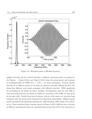
226. 198 Chapter 5. Spectral FE Analysis with Magnetostrictive Patches
Dispersion Relations
6
5
Group Speed (km/sec)
4
3
2
1
0
20 40 60 80 100 120 140 160 180
Frequency (kHz)
(a) Group Speed
10
8
Location (m)
6
4
2
0
0 1 2 3 4 5 6
Time (sec) x 10
−3
(b) Modulated Pulse Response
Figure 5.10: Group Speed and Modulated Pulse Response for [m/04 /904 /m] Layup with
U n = 1, W n = 0.

227. 5.4. Numerical Results and Discussion 199
Table 5.2: Propagation of modulated pulse with U n = 1, W n = 0 beam assumption.
m NBS Size (nano-m) Arrv. time (µ-sec) wave speed (m/sec)
0 21490 - - - - - - - -
1 29 20090 - 174 514 - 5736 1942 -
2 29 20110 - 346 862 - 5779 2318 -
3 29 20220 1340 525 1208 1438 5712 2483 2085
4 29 20190 1350 696 1553 1861 5739 2574 2148
5 29 20190 1350 875 1901 2284 5707 2629 2188
6 29 20080 1350 1047 2246 2707 5726 2670 2216
7 29 20050 1350 1226 2587 3130 5705 2705 2236
8 29 20200 1360 1398 2935 3553 5720 2725 2251
9 29 20260 1360 1570 3280 3976 5731 2743 2263
10 29 20220 1360 1751 3625 4399 5707 2757 2273
the Table-5.2. Considering the farthest measuring location from impact point gives the
best result among other measuring locations, axial, bending and shear wave speeds are
taken as 2757, 2273 and 5707 m/sec respectively. Corresponding amplitudes of the NBSs
are 20 µ-m for axial, 1.36 µ-m for bending and 29 nano-m for shear. It shows, although
the load is applied vertically, major component of vertical response is coming through
the axial wave mode. This is due to the asymmetric layup sequence, where the bending
stretching coupling produce axial mode due to vertical loading or bending mode due to
axial loading. Figure-5.11(a) and Figure-5.11(b) show the group speeds and response
Table 5.3: Propagation of modulated pulse with U n = 2, W n = 0 beam assumption.
m NBS Size (nano-m) Arrv. time (µ-sec) wave speed (m/sec)
0 21490 - - - - - - - -
1 20350 270 - 335 693 - 2977 1441 -
2 19390 270 - 678 1220 - 2945 1639 -
3 19490 270 - 1019 1744 - 2942 1719 -
4 19400 270 - 1352 2268 - 2956 1763 -
5 19590 270 - 1695 2792 - 2948 1790 -
6 19570 270 - 2039 3316 - 2942 1809 -
7 1820 19410 270 2187 2549 3833 3200 2745 1826
8 1820 19580 270 2501 2892 4357 3198 2765 1836
9 1810 19550 270 2815 3235 4883 3197 2781 1842
10 1810 19340 270 3121 3568 5407 3203 2802 1849
of modulated pulse with (U n = 2, W n = 0) beam assumption. Actual size of NBS at
each measuring locations are shown in Table-5.3. Locations of the NBSs are also given

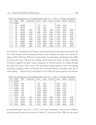
228. 200 Chapter 5. Spectral FE Analysis with Magnetostrictive Patches
Dispersion Relations
8
7
6
Group Speed (km/sec)
5
4
3
2
1
0
20 40 60 80 100 120 140 160 180
Frequency (kHz)
(a) Group Speed
10
8
Location (m)
6
4
2
0
0 1 2 3 4 5 6
Time (sec) x 10
−3
(b) Modulated Pulse Response
Figure 5.11: Group Speed and Modulated Pulse Response for [m/04 /904 /m] Layup with
U n = 2, W n = 0.

229. 5.4. Numerical Results and Discussion 201
in the same table. As before, from these location, velocity of the waves are calculated
and compared with the group speed obtained form the dispersion relationships. Different
group speeds calculated from the dispersion relations are as follows: 1954 (bending), 2790
(axial), 3296 (first shear), 7585 (second shear) m/sec. According to the dispersion curves
due to inclusion of another shear mode, axial, shear and bending speed is reduced from
2897, 5711 and 2366 to 2790, 3296 and 1954 m/sec respectively. From response shown
in Figure-5.11(a), second shear mode is not been captured due to very small amplitude.
Axial, bending and first shear waves speeds are calculated as 2802, 1849 and 3203 m/sec
respectively. Bending and axial NBS sizes are reduced to 270 nano-m and 19.34 µ-m
respectively where the first shear mode is increased to 1.81 µ-m.
Table 5.4: Propagation of modulated pulse with U n = 4, W n = 3 beam assumption.
m NBS Size (nano-m) wave speed (m/sec)
0 23200 - - - - - - - - -
1 20600 - - - - 3735 - - - -
2 29 23050 3680 - - 6957 2787 1588 - -
3 22420 3240 3250 260 - 3711 1910 1665 1539 -
4 22300 3230 3259 260 - 3717 1963 1705 1576 -
5 22190 3209 3250 260 - 3714 1995 1729 1595 -
6 22030 3190 3280 260 - 3711 2024 1749 1613 -
7 21740 3209 3240 260 - 3715 2040 1759 1624 -
8 21249 3220 3270 260 - 3717 2052 1770 1631 -
9 20690 3209 3259 260 - 3715 2061 1779 1639 -
10 250 20090 3200 1150 3259 1694 3488 2069 1834 1784
Figure-5.12(a) and Figure-5.12(b) show the group speeds and response of modulated
pulse with (U n = 4, W n = 3) beam assumption. Actual size of NBS at each measuring
locations are shown in Table-5.4. According to the dispersion curves, different group
speeds are 1693 (first contraction), 1842 (bending), 1894 (axial), 1923 (first shear), 2148
(second contraction), 3411 (second shear), 3717 (third contraction), 4646 (third shear),
6886 (fourth shear) m/sec. However, from the response shown in Figure-5.12(a), fourth
shear mode is captured only at 2m location and the NBS size is 29 nano-m. Third shear
mode is not captured in any of the location. Third contraction mode NBS size is 20.69
µ-m and the adjacent shear mode NBS is around one fifth of this. NBS size of first
contraction mode is 250 nano-m.
From this example, one can see the versatility of spectral element formulation in
graphically capturing all the propagating mode components for a beam structure.

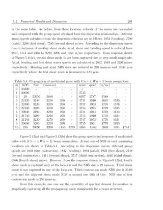
230. 202 Chapter 5. Spectral FE Analysis with Magnetostrictive Patches
Dispersion Relations
7
6
5
Group Speed (km/sec)
4
3
2
1
0
20 40 60 80 100 120 140 160 180
Frequency (kHz)
(a) Group Speed
10
8
Location (m)
6
4
2
0
0 1 2 3 4 5 6
Time (sec) x 10
−3
(b) Modulated Pulse Response
Figure 5.12: Group Speed and Modulated Pulse Response for [m/04 /904 /m] Layup with
U n = 4, W n = 3.

231. 5.4. Numerical Results and Discussion 203
5.4.1.5 Response to a Broad-band Pulse
In earlier section (Section-5.4.1.4), the modulated pulse was used to segregate different
propagating modes using an infinite beam. In this section a cantilever beam is con-
sidered which is subjected to broadband loading of 25 kHz (shown in Figure-5.13(a))
with a symmetric ([010 ]) and an asymmetric ([m/04 /904 /m]) layup sequences. The one-
dimensional spectral model of cantilever beam consists of a single element of one end fixed,
which results in a dynamic system matrix of size [3X3] for FSDT and [(2 + U n + W n)
X (2 + U n + W n)] for U n order of shear deformable with W n order of contraction beam
assumption, which need to be inverted at each frequency step. The force input for the
spectral analysis is triangular pulse sampled at a time step of 0.244µ-sec using 16384 FFT
points. The load is applied vertically at the free end of the beam and the vertical velocity
(of any point on the reference plane, i.e., the mid-depth of the composite layer) at the
same point is measured and plotted in Figure-5.13(b) for [010 ] layup sequence. In this fig-
ure, the peak amplitude at 0.26 milli-sec is the incident part of the pulse. The wave then
propagates towards the fixed end and gets reflected at the boundary and this reflection
appears at around 0.5 milli-sec. As is seen in the figure, the higher order elements have
a difference in the occurrence of reflection from the boundary. This is expected, since the
dispersion relation suggests that the bending speed for FSDT is higher than the other
higher order beam assumptions. In addition, as the shear cut off frequency for [010 ] layup
is beyond 25 kHz and due to symmetric layup sequence, bending-stretching coupling is
absent, only bending mode is propagating for this loading.
Figure-5.14 shows the tip vertical velocity and sensor response histories of a can-
tilever beam with [m/04 /904 /m] layup sequence due to vertical impact load shown in
Figure-5.13(a) at the tip of the cantilever. Figure-5.14(a) shows the cantilever tip ve-
locity for [m/04 /904 /m] layup sequence. Response behavior is seen to be similar to the
previous case. However, there is significant difference in the voltages predicted by different
beam theories. This is shown in Figure-5.14(b).
In this section, mechanical response as well as sensor response histories due to impact
load is studied for a cantilever beam. Some of the observations in Section-5.4.1.3 were
verified here. More importantly, it was found that, increase in the order of beam theory
reduces the effective group speeds. In the next section, impact load will be reconstructed
from the response histories of the sensor, which is called the force identification problem.

232. 204 Chapter 5. Spectral FE Analysis with Magnetostrictive Patches
1
−5
x 10
0.9
4
0.8
3.5
Frequency Content
0.7 3
0.6 2.5
Force (N)
2
0.5
1.5
0.4 1
0.3 0.5
0.2 0 20 40 60
Frequency (kHz)
0.1
0
0 200 400 600 800 1000
Time (µ sec)
(a) Broadband pulse of 25 kHz with Frequency content (inset)
−5
x 10
Un=1, Wn=0
16 Un=2, Wn=1
Un=3, Wn=2
Un=4, Wn=3
14
12
Velocity (m/sec)
10
8
6
4
2
0
0 0.2 0.4 0.6 0.8 1 1.2
Time (sec) x 10
−3
(b) Vertical velocity at Cantilever Tip
Figure 5.13: Broadband response of 010 layup sequence.

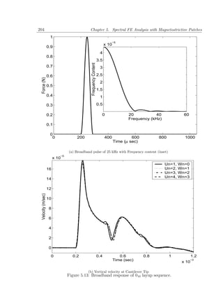
233. 5.4. Numerical Results and Discussion 205
−5
x 10
15
Un=1, Wn=0
Un=2, Wn=1
Un=3, Wn=2
Un=4, Wn=3
10
Velocity (m/sec)
5
0
0 0.2 0.4 0.6 0.8 1 1.2
Time (sec) x 10
−3
(a) Vertical velocity at Cantilever Tip
0.14 Un=1, Wn=0
Un=2, Wn=1
Un=3, Wn=2
0.12
Un=4, Wn=3
0.1
Open Circuit Voltage (V)
0.08
0.06
0.04
0.02
0
−0.02
0 0.2 0.4 0.6 0.8 1 1.2
Time (sec) x 10
−3
(b) Sensor Open Circuit Voltage history
Figure 5.14: Broadband response of [m/04 /904 /s] layup sequence (s for sensor layer).

234. 206 Chapter 5. Spectral FE Analysis with Magnetostrictive Patches
5.4.2 Force Identification
Force identification is a class of inverse problem where in, the measured response and
system transfer functions are used to reconstruct the force. This is a very challenging
problem, which can be elegantly handled using the formulated spectral element.
The mechanical force acting on a body cannot be measured directly. If a body is
loaded statically and if the body deforms linear-elastically, the deformation at any point
of the body is proportional to the applied force. Therefore, the variation of the force
can be measured indirectly by measuring the variation of the deformation. However, this
principle cannot be applied when a body is subjected to a dynamic force. In this case,
the propagation of stress waves inside the body should be considered so that the variation
of the deformation at any point of the body is no longer the same as the variation of
the applied force. Hence, dynamic force is much more difficult to measure than static
force. In order to overcome this difficulty, inverse analysis methods to estimate variations
of impact force from measured responses of a body have been studied extensively during
the last two decades. Inoue et al. [166] presented a review of methods of inverse analysis
for the indirect measurement of impact force. Stevens [346] presented an overview of the
force identification process for the case of linear vibration systems, and classified them
into discrete systems and continuous systems.
The measurement of dynamic forces acting on structures or machines is frequently
impossible due to accessibility problems related to transducer placement. A seemingly
simple way to solve this problem is to determine the transfer function of the system,
measure the system vibration, and back-calculate the forces that produced the vibration.
When the FRF matrix describing the dynamical behavior of a structure is available, the
operational loads can be determined by multiplying the pseudo-inverse of the FRF matrix
by the operational responses (displacements, velocities or accelerations). Unfortunately,
the nature of this ”inverse problem” is mathematically ill-conditioned, i.e. small mea-
surement errors lead to large errors in predicted forces. In early papers, Doyle [104, 105]
used a frequency-domain deconvolution technique to estimate the impact force on beams
and plates from strain gauge measurements. The Fast Fourier Transform (FFT) was used
to convert the measured strain history into its frequency components, which were used
to obtain the frequency components of the impact force. Then the Inverse Fast Fourier
Transform (IFFT) was implemented to reconstruct the impact force history in the time-
domain. Doyle [106] demonstrated the reconstruction of impact force of a two-dimensional
bimaterial beam system. In another paper, Doyle [107] introduced a computationally ef-

235. 5.4. Numerical Results and Discussion 207
ficient deconvolution method with similarities to Fourier analysis and wavelet analysis for
force reconstructions using measured acceleration responses from beam and plate models.
Martin and Doyle [254] used a frequency domain deconvolution method to clarify some
of the fundamental difficulties and issues involved in the inverse problem of solving for
the impact force history using experimentally measured structural responses. Recently,
Adams and Doyle [5] presented a method for determining force histories using experi-
mentally measured responses which can determine multiple isolated (uncorrelated) force
histories as well as distributed pressures and tractions and allows for the data collected
being of dissimilar type. As a demonstration of the method and of its scalability, force
reconstructions for an impacted shell and an impacted plate were determined using ac-
celerometer and strain gage data. Chakraborty and Gopalakrishnan [61] used spectral
finite element to reconstruct the force history applied to a functionally graded material.
Mitra and Gopalakrishnan [271] used spectrally formulated wavelet finite element for
impact force identification in connected 1-D waveguides.
Instead of obtaining the impact force history through the direct deconvolution pro-
cess of a convolutional integral, Wu et al. [405, 406] developed a constrained optimization
technique to detect the impact force history exerted on a laminated composite plate from
the recorded strain responses. A Green’s function was constructed based on the classical
lamination theory and the model superposition method to correlate the laminate response
to the impact force. To obtain the impact force histories exerted at multiple locations on
the laminate, a constrained optimization method is employed. Chang and Sun [70], on
the other hand, used experimentally generated Green’s functions and time-domain decon-
volutions to estimate the impact force history from strain measurements. A least-square
fit method was used in their numerical scheme. However, the amplitudes of the Green’s
functions had to be scaled to account for different impactor characteristics. Hollandsworth
and Busby [159] used experimental measurement data to describe the velocity response
of an impacted cantilever beam to the problem of impact force identification. A spectrum
analyzer was used to measure the beam accelerations within 40 µ-sec time intervals and
the accelerations were integrated for velocity in the inverse algorithm. Predicted impact
force given by the inverse technique was compared with actual dynamic load of impact
hammer. Wu et al. [404] presented two methods for the purpose of detecting the impact
force history. In the first method, the classical plate theory, and the normal-mode super-
position method using Bessel functions were used to construct Green’s functions in the
time-domain. A constrained optimization technique was used to reconstruct the impact

236. 208 Chapter 5. Spectral FE Analysis with Magnetostrictive Patches
force history from measured strain histories. This method was limited to axisymmet-
ric impact problems because of the restriction of the Green’s functions. In the second
method, the impact force history was reconstructed using the gradient projection method
by comparing the response to recorded force and strain histories of a controlled impact.
Tsai et al. [373] also used a Green’s function approach to estimate impact force from
experimental data on sandwich panels. Huang et al. [163] described an inverse technique
for the prediction of impact forces from acceleration measurements on a vibratory ball mill
with a method based on an optimization approach. Yang [413] used linear least-squares
method to estimate the force on one end of a bar in the one-dimensional inverse vibration
problem. Finite-difference method was employed to discretize the problem domain, and
then a linear inverse model is constructed to identify the force condition. Briggs and
Tse [48] proposed a technique to determine the magnitude and location of impact forces
on a structure from extracted modal constants and a pattern matching procedure. Ma
et al. [239] presented an on-line recursive inverse method to estimate the input forces
of beam structures based on the Kalman filter and a recursive least-squares algorithm.
In the numerical experiments, the cantilever beam was subjected to five types of input
forces, i.e., sinusoidal, triangular impulse, rectangular impulse, a series of impulses and
random. In another paper, Ma and Ho [240] proposed an inverse method to identify in-
put forces of non-linear structural systems using extended Kalman filter and a recursive
least-squares estimator. Flores et al. [122] presented an inverse procedure for the deter-
mination of external loads, given the dynamic responses of the loaded structure and its
corresponding finite element model using particle swarm optimization together with the
Lagrange-Newton sequential quadratic programming method. Cruz et al. [92] presented
a nonlinear least-square method for determining the location and magnitude of a static
point force acting on a plate from a number of displacement readings at discrete points on
the plate. Chock and Kapania [80] identified the loads on the finite element model that
would create equivalent displacements or stresses by various means, thus saving a large
amount of computational effort using methods based on classical least-squares methods.
Christoforou et al. [87] presented an inverse model for estimation of the mass and ve-
locity of the impactor in low-velocity impact of composite plates using a least-squares
optimization technique for optimal reconstruction of the force-time history. Odeen and
Lundberg [295] established a method which permits prediction of impact force history
from the velocity response of each impacting body to an impulsive force applied to its
impact face, and the impact velocity.

237. 5.4. Numerical Results and Discussion 209
Force identification from dynamic responses of bridges is an important inverse prob-
lem. The parameters of both the vehicle and the bridge play an important role in the
force identification. Based on the bending moments measured in the laboratory, Chan
et al. [69] developed four different identification methods in the moving force identifica-
tion system of the bridges. Law and Fang [211] applied dynamic programming technique
for moving forces identification. Busby and Trujillo [51] estimated the unknown forcing
function using an eigenvalue reduction technique, in conjunction with inverse dynamic
programming. They showed that the input force history can be reconstructed by solving
a dynamic inverse problem. Hollandsworth and Busby [159] used acceleration measure-
ments to identify the impact force on aluminum beams by solving a dynamic inverse
problem experimentally. In the experiment, the load was applied at a known position and
accelerometers were used as sensors. For an unknown loading point, Cruz et al. [92] for-
mulated a nonlinear inverse problem and tried to find the location and magnitude of the
external force. The force, however, was not general but confined to a sinusoidal function
whose amplitude and phase are the only parameters to be found.
With the advent of smart structure technology, Choi and Chang [82] proposed
an impact load identification method using distributed built-in piezoelectric sensors for
detecting foreign object impact. Their identification process consisted of a system model
and a response comparator, employing a quasi-Newton procedure to estimate the location
of impact, and the least-square fit method to predict the force history. Lihua and Baoqi
[228] used neural networks and piezoelectric sensors to identify the location and amplitude
of a static force on a square plate.
In the earlier section (Section-5.4.1.5), the relation between force histories and open
circuit voltages in sensor was formulated based on the spectral finite element method for
a broadband impact event. The sensor responses are described as a product of transpose
matrix and force histories. In this section, from open circuit voltage histories of magne-
tostrictive sensor, impacted force histories in a laminated composite beam is identified
using spectral finite element formulation.
Inherent advantage of the spectral element in the solution of inverse problems is
utilized here to reconstruct the force history applied to a composite beam. In the absence
of experimental data, truncated sensor response histories are used as surrogate experi-
mental responses. These truncated responses are given as input to spectral element solver
and the force data are reconstructed by performing inverse analysis. Since, experimental
outputs are always truncated at some point depending upon constraints of the setup,

238. 210 Chapter 5. Spectral FE Analysis with Magnetostrictive Patches
data acquisition system and other facilities, the surrogate response should be such that
it simulates the experimental results realistically. When this truncated response is given
as input to the spectral solver, the force data can be reconstructed by performing inverse
analysis. The Fast Fourier Transform is used for inversion to the time domain. As the
whole formulation is done in the frequency domain, a straight forward relationship exists
between transformed input and transformed response through the system transfer func-
tion. Also, in the spectral element method, the governing equation is solved exactly, so
that the exact transfer function is obtained, which can be used to obtain the force input.
Since the whole spectral formulation is in the frequency domain, the response is related
to the input through the transfer function in the frequency domain as:
ˆ ˆ ˆ
Y (ω) = H(ω)X(ω)
ˆ ˆ
where, X(ω) is the transformation of the input (say, load), Y (ω) is the transform of the
ˆ
output (typically, velocity, strain etc. Here, open circuit voltages), and H(ω) is the system
transfer function for a particular frequency ω. The input force can be obtained easily by
dividing the transform of the response by the transfer function, i.e.,
ˆ ˆ ˆ
X(ω) = Y (ω)/H(ω)
Thus, if the response of a sensor is known, then the disturbance that caused it can be
computed. This is one of the distinct advantages of the spectral approach in its ability to
ˆ
solve inverse problems. In general, Y will be experimental data, (here transform of voltage
history). The experimental outputs are always truncated at some point. This is the reason
why the output is also truncated here to simulate the experimental environment. Next,
details of the numerical experiment for force identification are outlined.
A cantilever beam of 0.5m length is taken for this purpose. A single element is used
to model this beam along with one throw-off element to take away unwanted reflections.
An impulse load is applied at tip of the cantilever as shown in Figure-5.13(a). The load
has frequency content of about 25 kHz and duration of 100 µ sec. Sensor response of the
beam (open circuit voltages) due to this loading, as obtained from the analysis by previous
section (5.4.1.5) is shown in Figure-5.14(b). The response is truncated at various points
in time history as shown in Figure-5.15(a), where the open circuit voltages in the sensor
are plotted. This truncated response is transformed in the frequency domain and used
in spectral solver for inverse analysis. Figure-5.15(b) shows the force histories generated
for different truncated responses. As seen in the figure, all the truncated responses can

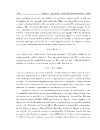
239. 5.4. Numerical Results and Discussion 211
0.1 4 mili−sec
0.05
Open Circuit Voltage (V)
0
0 0.5 1 1.5 2 2.5 3 3.5 4
0.1 2 mili−sec
0.05
0
0 0.5 1 1.5 2 2.5 3 3.5 4
0.1 1 mili−sec
0.05
0
0 0.5 1 1.5 2 2.5 3 3.5 4
0.1 500 µ−sec
0.05
0
0 0.5 1 1.5 2 2.5 3 3.5 4
Time (mili−sec)
(a) Sensor Response truncated at several points
1
4 mili−sec
0.5
Reconstructed Force (N)
0
0 0.5 1 1.5 2 2.5 3 3.5 4
1
2 mili−sec
0.5
0
0 0.5 1 1.5 2 2.5 3 3.5 4
1
1 mili−sec
0.5
0
−0.5
0 0.5 1 1.5 2 2.5 3 3.5 4
1
500 µ−sec
0.5
0
−0.5
0 0.5 1 1.5 2 2.5 3 3.5 4
Time (mili−sec)
(b) Reconstructed Force history from several truncated sensor responses
Figure 5.15: 25 kHz Broadband Force Reconstruction for [m/04 /904 /m] layup.

240. 212 Chapter 5. Spectral FE Analysis with Magnetostrictive Patches
predict the original pulse quite accurately and the main difference occurs in subsequent
part of the load. This spurious parts are due to the shortcoming of FFT in limited time
window. Reconstructed forces corresponding to 4 mili-sec response history, predicted the
force history exactly. However, forces corresponding to truncation point of 2 mili-sec show
kinks at about 1.5 to 3 mili-sec and some of them are negative, which can be discarded
using intelligent postprocessing. This example shows that if truncation point is about 1
mili-sec, comparable force history can be reconstructed. For truncation point of about
500 µ-sec, unacceptable spurious part appears in the force history, which are difficult to
evaluate in postprocess. Overall, the example shows the efficiency of the spectral method
in force identification.
5.5 Summary
A new spectral finite element for composite beam with magnetostrictive patches is de-
veloped, which takes higher order of shear deformation and higher order of Poisson’s
contraction into account. The formulation of the spectral element is performed using a
general procedure. The extra propagating modes due to the presence of higher order
assumption are captured successfully by the element. The effect of the higher orders on
the spectrum and dispersion relation is shown in detail. Expressions for first few cut-off
frequencies are given in closed form, which determines the required order of beam assump-
tion for analysis depending upon the loading frequency. It is shown how the response of
a structure is altered due to the higher order assumption, which is quite significant at
high frequencies. Magnetostrictive sensor response due to broadband impact force in the
composite cantilever is computed. Finally, as a study of structural health monitoring, the
element in association with truncated sensor open circuit voltages (used as a replacement
of experimental data) when subjected to high frequency impact loading is instrumental
in reconstructing the force to which the structure was subjected. It has been shown that
the force can be reconstructed without any period error.

241. Chapter 6
Forward SHM for Delamination
6.1 Introduction
Composite is changing the world of structural construction due to its various technological
advantages. However, these new materials also have some problems such as fiber breakage,
matrix cracking, and delamination. Matrix cracks and fiber breakages play an important
role in laminates under tensile load. But, the primary concern with polymer composites is
the delamination failure, which is debonding of adjacent plies, since the through-thickness
properties of composite laminates are typically matrix dominated and therefore, much
weaker than the fiber dominated in-plane properties. In industry, one of the commonly
encountered types of defect or damage in laminated composite structures is delamination.
Delamination often occur at stress free edges due to the mismatch of properties at ply
interfaces and it can also be generated by external forces such as out of plane loading or
impact during the service life. While such impact can cause a number of delaminations, a
small surface indentation is the only external indication since the delaminations are cracks
in the interior of the laminate. Thus, this type of damage is often called barely visible
impact damage, which is not readily identified by visual inspection. This problem is
caused from the fact that transverse tensile and interlaminar shear strength of composite
laminates are quite low in contrast to their in-plane properties. Inter layer debonding or
delamination is a prevalent form of damage phenomenon in laminated composites. It may
be formed due to a wide variety of foreign object impact damage, poor fabrication process,
and fatigue from environmental cycling. Delaminations cause a reduction in the stiffness
of the structure thus affecting its vibration characteristics. They also substantially reduce
the buckling load capacity, which, in turn, influences the stability characteristics of the
structure. Hence, delamination is the critical parameter for laminates under compression
and one of the most common failure modes in composite laminates. Kim et al. [183]
213

242. 214 Chapter 6. Forward SHM for Delamination
had studied the effects of delaminations in composite plate. Delamination of composite
laminate had been studied in structural health monitoring context by many researchers
[72, 234, 247, 285, 332, 348, 350, 352, 370, 418].
In this chapter, numerical simulation are carried out for a delaminated composite
laminate with or without magnetostrictive patches as sensors and actuators using anhys-
teretic, coupled, linear properties of magnetostrictive materials. Effect of delamination in
cantilever tip velocity and sensor open circuit voltages are studied. Single and multiple
delaminations are studied with tip vertical impact load and biased sinusoidal current in
actuator coil. The presence of delamination, changes the stress response of the struc-
ture. This in turn changes the magnetic flux density of the magnetostrictive sensor. The
changes in the flux density are sensed through a sensing coil as open circuit voltage. Mea-
surement of open circuit voltage before and after the damage (delamination) occurrence
provides a diagnostic measure to indicate the presence of the damage.
This chapter is organized as follows. First the modelling of delamination consid-
ering beam and 2D plane stress formulation is studied and compared for both static tip
deflection and natural frequencies of a cantilever beam. Then the tip deflection histories,
due to tip vertical load on a delaminated cantilever beam are studied for different size and
location of delamination. Next, due to the same tip load, sensor open circuit voltages are
studied for different delamination configurations. To study the effect of location of sensor
in response histories, one delaminated portal frame is studied with different locations of
sensors with a fixed location of delamination and actuator. Although beam assumption
reduces the computational cost, it introduces the errors from its inherent assumption.
The relative importance between the errors due to different beam assumptions and the
sensitivity of the delamination for both thick and thin portal frame is studied. Finally,
the effect of different delamination configuration on tip deflection and sensor response due
to actuation in two different frequencies are studied. The chapter is then concluded with
a brief summary.
6.2 Delamination Modelling in Composite Laminate
Many stiffness and modulus degradation models have been proposed in the literature
for finite element modelling of damage, which is not suitable for modelling of delamina-
tion in composite structure. Literature for modelling of delamination is discussed in the
introductory chapter of Section-1.2.5.2.

243. 6.2. Delamination Modelling in Composite Laminate 215
10 11 12 13 14
11 12 13 14
1 2 8 9
1 2 3 4 5 6 7 8 9 10
3 4 5 6 7
Beam
1 2 3 4 5 6 7 8 9 10
1 2 3 4 5 6 7 8 9
24 25 26 27
21 22 23 31 32 33 34 28 29 30
10 11 12 13 14 15 16 17 18
11 12 13 14 15 16 17 18 19 20
2D Plane Stress/Strain
Figure 6.1: Modelling of Delamination in Finite Element Formulation.
In this chapter, modelling of delamination in finite element is done through keeping
two nodes in same place, one for the elements above the delamination and other for
below. Modelling of delamination for beam and 2D plane stress/ plane strain assumption
is shown in Figure-6.1. For beam formulation, elements 1 and 2 are at the left part,
and, elements 8 and 9 are at the right part of the delaminated zone. All other elements
are in the delaminated zone, either at the above or below the delamination. Zone below
the delamination is modelled with elements 3 to 7 and above by elements 10 to 14.
Delamination is modelled through proper nodal connectivity of these elements. That is,

244. 216 Chapter 6. Forward SHM for Delamination
for healthy zone, element 1 is connected with nodes 1 and 2; and element 9 is connected
with nodes 9 and 10. All these nodes are in the mid plane of the corresponding beam
elements. For element below the delamination, like, element 3 is connected with nodes
3 and 4, where, the nodes 3 and 4 are not in the mid plane of this element. This may
create high bending-stretching coupling. Similarly, for element above the delamination,
like, element 10 is connected through nodes 3 and 11, where nodes 3 and 11 are not
in the mid plane of this element. As mention earlier, nodes 4 and 11 are in the same
place and not connected with any direct element. These are termed as duplicate nodes.
Similarly, (5 and 12), (6 and 13) and (7 and 14) nodes are the duplicate nodes. In the
delaminated zone, lower part of the elements connects with nodes 4, 5, 6, and 7 and upper
parts of the elements connect nodes 11, 12, 13, and 14. If these nodes are merged with
their corresponding duplicate nodes, the beam will be healthy. In addition, with these
duplicate nodes, different kind of contact or gap elements can be used in finite element
analysis.
In the literature, for 2D plane stress/strain assumption, delamination is modelled
using such duplicate nodes. Nodes 24, 25, 26 and 27 are connected with the elements
for above the delamination, and their corresponding duplicate nodes are 31, 32, 33 and
34, which are connected with elements below of the delamination respectively. Elements
below the delamination, like element 12 is connected with nodes 13, 14, 31 and 23, and
elements above the delamination, like element 3 is connected with nodes 23, 24, 4 and
3. These two elements have duplicate nodes 24 and 31. Similarly, (25, 32), (26, 33) and
(27, 34) are duplicate nodes for other elements exist below and above the delamination.
Multiple delaminations can also be modelled in similar manner for both beam and 2D
assumption. Static and free vibration study for a unidirectional laminated cantilever
beam is performed to demonstrate the efficiency of the present delamination modelling
strategy.
Figure-6.2(a) shows the percentage increase of static tip deflection due to mid layer
delamination near the support of a cantilever beam. When the delamination is 10 % of the
length of the cantilever, beam assumption shows 0.39% of increase of static tip deflection.
But when the 90% of the cantilever is delaminated, the increase of static tip deflection
is 55.16%. Corresponding percentage increase of deflection due to 2D model is 0.3% to
0.4% lower than the beam formulation. Hence, it clearly indicates, present delamination
model of beam can be used for static analysis with in 0.5% accuracy.
Figure-6.2(b) shows the decrease of first 15 natural frequencies due to mid layer

245. 6.2. Delamination Modelling in Composite Laminate 217
60
Beam
Plane Stress
50 Delam(%) Beam Plane Stress/Strain
10 00.39 00.08
% Increase of Static Deflection
20 00.91 00.61
40 30 02.35 02.03
40 05.15 04.80
50 09.77 09.37
60 16.63 16.24
30
70 26.13 25.75
80 38.90 38.32
90 55.16 54.60
20
10
0
0 10 20 30 40 50 60 70 80 90
Delamination (%)
(a) Static Tip Deflection
0
−10
% Reduction of Natural Frequencies
−20
−30
−40
−50
−60
−70
Beam
−80 Plane Stress
0 10 20 30 40 50 60 70 80 90
Delamination (%)
(b) Free Vibration
Figure 6.2: Comparison between Beam and 2D Modelling of Delamination

246. 218 Chapter 6. Forward SHM for Delamination
delamination near the support of a cantilever beam. Both the models (beam and 2D)
show more or less similar results. When the delamination is 10 % of the length of the
cantilever, 15th natural frequency reduces 20% than the corresponding frequency of the
healthy beam. Similarly, for 90% delamination, first natural frequency reduces 29%,
second natural frequency reduces 40% and third natural frequency reduces 72%. This
study shows that the results of static and dynamic simulations for beam and 2D-plane
stress/strain models give results that match very well. In the next section, with this
modelling technique of delamination, structural responses of a delaminated cantilever
beam are studied.
6.3 Numerical Example
Figure 6.3: Composite Beam with Sensor and Actuator
In this section, a cantilever beam is considered to explore the use of magnetostric-
tive sensors and actuators for a time domain health monitoring application. Numerical
simulation is carried out by assuming a unidirectional laminated composite beam of to-
tal thickness 1.8mm as shown in Figure-6.3. Length and width of the beam is 500mm
and 50mm respectively. The beam is made of 12 layers with thickness of each layer be-
ing 150 µ-m. Position of sensor and actuator are fixed at top and bottom layer of the

247. 6.3. Numerical Example 219
beam respectively. Both the sensor and actuator are placed near the support of the can-
tilever. Size of the actuator and sensor are 50mmX50mm with 150 µ-m thickness. Elastic
modulus of composite is 181 GPa and 10.3 GPa in parallel (E1 ) and perpendicular (E2 )
direction of fiber. Poisson’s ratio (ν), density (ρ) and shear modulus (G12 ) of composite
is assumed 0.0, 1.6 gm/c.c. and 28 GPa respectively. Elastic modulus (Em ), Poisson’s
ratio (νm ), shear modulus (Gm ) and density (ρm ) of magnetostrictive material is 30 GPa,
0.0, 23 GPa and 9.25 gm/c.c. respectively. Magneto-mechanical coupling coefficient is 15
nano-m/amp for sensing and actuation properties of magnetostrictive material. Relative
permeability of magnetostrictive material has been considered as 10. Number of coil turn
in sensor and actuator are 20000 turn/m (1000 turn).
Figure-6.4 to Figure-6.16 are the response histories for different delaminated and
healthy cantilever beam. Continuous lines are the response for healthy and dotted lines
are for delaminated beam. Cantilever beam showing delamination with position and size
is plotted in the inset of the corresponding figures.
6.3.1 Tip Response Due to Tip Load
Figure-6.4 to Figure-6.10 are the vertical velocity histories due to vertical load in the
tip of the cantilever. Load history and its frequency content are shown in the Figure-
5.13(a). For healthy beam, waves reflected from support and arrived after 1 mili-sec. For
delaminated beams, these waves will be scattered from delamination tip and reflected back
from the delaminated zone. Hence from the arrival time of the reflected wave, location of
delamination zone can be identified. Similarly, the deviation of the response from healthy
beam response gives some information about the size of the delamination. If the deviation
is more delamination size is more.
6.3.1.1 Varying Location
Figure-6.4 shows the cantilever tip velocity for 100mm delamination at mid layer and
for different distance from support (0, 80, 160, 240, 320, and 400mm). As mentioned
earlier the reflected waves arrived much earlier for delamination near the tip than for
delamination near the support. For delamination near the support, difference of the
responses starts from 1 milli-sec. But when the delamination is at the free end (400mm
from support) of the cantilever, response difference start from 0.35 milli-sec.
Figure-6.5 shows the cantilever tip velocity for 20mm delamination at mid layer and
for different distance from support (0, 80, 160, 240, 320, and 400mm). As pointed out in

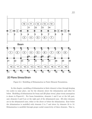
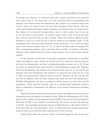
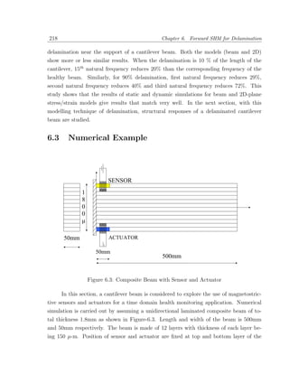
248. 220 Chapter 6. Forward SHM for Delamination
0.025 0.025
0.02 0.02
0.015 0.015
Velocity (m/sec)
Velocity (m/sec)
500mm [012] 500mm [012]
0.01 0.01
0.005 0.005
0 0
−0.005 −0.005
0 0.5 1 1.5 2 0 0.5 1 1.5 2
Time (sec) −3
x 10 Time (sec) −3
x 10
0.025 0.025
0.02 0.02
0.015 0.015
Velocity (m/sec)
Velocity (m/sec)
500mm [012] 500mm [012]
0.01 0.01
0.005 0.005
0 0
−0.005 −0.005
0 0.5 1 1.5 2 0 0.5 1 1.5 2
Time (sec) −3
x 10 Time (sec) −3
x 10
0.025 0.025
0.02 0.02
0.015 0.015
Velocity (m/sec)
Velocity (m/sec)
500mm [012] 500mm [012]
0.01 0.01
0.005 0.005
0 0
−0.005 −0.005
0 0.5 1 1.5 2 0 0.5 1 1.5 2
Time (sec) −3
x 10 Time (sec) −3
x 10
Figure 6.4: 100mm Delamination at Mid Layer and Different Distance from Support.

249. 6.3. Numerical Example 221
0.025 0.025
0.02 0.02
0.015 0.015
Velocity (m/sec)
Velocity (m/sec)
500mm [012] 500mm [012]
0.01 0.01
0.005 0.005
0 0
−0.005 −0.005
0 0.5 1 1.5 2 0 0.5 1 1.5 2
Time (sec) −3
x 10 Time (sec) −3
x 10
0.025 0.025
0.02 0.02
0.015 0.015
Velocity (m/sec)
Velocity (m/sec)
500mm [012] 500mm [012]
0.01 0.01
0.005 0.005
0 0
−0.005 −0.005
0 0.5 1 1.5 2 0 0.5 1 1.5 2
Time (sec) −3
x 10 Time (sec) −3
x 10
0.025 0.025
0.02 0.02
0.015 0.015
Velocity (m/sec)
Velocity (m/sec)
500mm [012] 500mm [012]
0.01 0.01
0.005 0.005
0 0
−0.005 −0.005
0 0.5 1 1.5 2 0 0.5 1 1.5 2
Time (sec) −3
x 10 Time (sec) −3
x 10
Figure 6.5: 20mm Delamination at Mid Layer and Different Distance from Support.

250. 222 Chapter 6. Forward SHM for Delamination
the earlier Figure, the reflected waves arrived much earlier for delamination near the tip
than for delamination near the support. Comparing Figure-6.4 and Figure-6.5 it is clear
that the deviation of response for delaminated beam from response of healthy beam is
more if the size of the delamination is more.
6.3.1.2 Varying Size
Figure-6.6 shows the responses for different sizes (10, 20, 30, 50, 75, 100mm) of delam-
ination at mid span and at the middle layer of the beam. For 10mm delamination, the
deviation is negligible, where as for 100mm delamination, deviation is quite large. In
addition, disturbance in the response for reflection from support is less for the smaller
delamination. The initial deviation of the response histories are always appear in the
same time of the response, which clearly indicate that the location of the delamination is
same for all the cases.
Depth wise location of the delamination will also affect the baseline response.
Figure-6.7 shows the responses of a delamination of varying size and located at top layer
of the beam. Although the reflection arrival time is similar to the response of mid layer
delamination, the magnitude of the deviation from the healthy beam response is smaller.
However, within the layer, if the size of delamination is increased, the amplitude of the
deviation of response form healthy response is also increased. Hence, if delamination
layer is identified, size of the delamination can be identified from the magnitude of the
deviation of the responses. Moreover, the initial appearance of the disturbance in time
history clearly indicates that the location of the delamination is same for all the cases.
6.3.1.3 Symmetric Delaminations
Figure-6.8 and Figure-6.9 show the response histories for different size (10, 20, 30, 50, 75,
100mm) of symmetric delaminations at the mid span of the beam. Figure-6.8 shows the
response history for two delaminations at mid span of the beam, one at top layer and
other in bottom layer. Initial reflections from delamination in response history for this
symmetric delamination is increased up to 30mm delamination size and again reduced for
longer delaminations. The disturbance of reflection from support is increased for increased
size of delamination.
Figure-6.9 shows the response histories for the symmetric delamination, which
makes three equal depth beams at delaminated zone. Here, the effect of delamination
in response histories are more, even for 10mm delamination sizes. Moreover, the distur-

251. 6.3. Numerical Example 223
0.025 0.025
0.02 0.02
0.015 0.015
Velocity (m/sec)
Velocity (m/sec)
500mm [012] 500mm [012]
0.01 0.01
0.005 0.005
0 0
−0.005 −0.005
0 0.5 1 1.5 2 0 0.5 1 1.5 2
Time (sec) −3
x 10 Time (sec) −3
x 10
0.025 0.025
0.02 0.02
0.015 0.015
Velocity (m/sec)
Velocity (m/sec)
500mm [012] 500mm [012]
0.01 0.01
0.005 0.005
0 0
−0.005 −0.005
0 0.5 1 1.5 2 0 0.5 1 1.5 2
Time (sec) −3
x 10 Time (sec) −3
x 10
0.025 0.025
0.02 0.02
0.015 0.015
Velocity (m/sec)
Velocity (m/sec)
500mm [012] 500mm [012]
0.01 0.01
0.005 0.005
0 0
−0.005 −0.005
0 0.5 1 1.5 2 0 0.5 1 1.5 2
Time (sec) −3
x 10 Time (sec) −3
x 10
Figure 6.6: Delamination at Mid span of Mid Layer with Different sizes.

252. 224 Chapter 6. Forward SHM for Delamination
0.025 0.025
0.02 0.02
0.015 0.015
Velocity (m/sec)
Velocity (m/sec)
500mm [012] 500mm [012]
0.01 0.01
0.005 0.005
0 0
−0.005 −0.005
0 0.5 1 1.5 2 0 0.5 1 1.5 2
Time (sec) −3
x 10 Time (sec) −3
x 10
0.025 0.025
0.02 0.02
0.015 0.015
Velocity (m/sec)
Velocity (m/sec)
500mm [012] 500mm [012]
0.01 0.01
0.005 0.005
0 0
−0.005 −0.005
0 0.5 1 1.5 2 0 0.5 1 1.5 2
Time (sec) −3
x 10 Time (sec) −3
x 10
0.025 0.025
0.02 0.02
0.015 0.015
Velocity (m/sec)
Velocity (m/sec)
500mm [012] 500mm [012]
0.01 0.01
0.005 0.005
0 0
−0.005 −0.005
0 0.5 1 1.5 2 0 0.5 1 1.5 2
Time (sec) −3
x 10 Time (sec) −3
x 10
Figure 6.7: Delamination at Mid span of Top Layer with Different sizes.

253. 6.3. Numerical Example 225
0.025 0.025
0.02 0.02
0.015 0.015
Velocity (m/sec)
Velocity (m/sec)
500mm [012] 500mm [012]
0.01 0.01
0.005 0.005
0 0
−0.005 −0.005
0 0.5 1 1.5 2 0 0.5 1 1.5 2
Time (sec) −3
x 10 Time (sec) −3
x 10
0.025 0.025
0.02 0.02
0.015 0.015
Velocity (m/sec)
Velocity (m/sec)
500mm [012] 500mm [012]
0.01 0.01
0.005 0.005
0 0
−0.005 −0.005
0 0.5 1 1.5 2 0 0.5 1 1.5 2
Time (sec) −3
x 10 Time (sec) −3
x 10
0.025 0.025
0.02 0.02
0.015 0.015
Velocity (m/sec)
Velocity (m/sec)
500mm [012] 500mm [012]
0.01 0.01
0.005 0.005
0 0
−0.005 −0.005
0 0.5 1 1.5 2 0 0.5 1 1.5 2
Time (sec) −3
x 10 Time (sec) −3
x 10
Figure 6.8: Symmetric Delaminations at Top and Bottom Layers.

254. 226 Chapter 6. Forward SHM for Delamination
0.025 0.025
0.02 0.02
0.015 0.015
Velocity (m/sec)
Velocity (m/sec)
500mm [012] 500mm [012]
0.01 0.01
0.005 0.005
0 0
−0.005 −0.005
0 0.5 1 1.5 2 0 0.5 1 1.5 2
Time (sec) −3
x 10 Time (sec) −3
x 10
0.025 0.025
0.02 0.02
0.015 0.015
Velocity (m/sec)
Velocity (m/sec)
500mm [012] 500mm [012]
0.01 0.01
0.005 0.005
0 0
−0.005 −0.005
0 0.5 1 1.5 2 0 0.5 1 1.5 2
Time (sec) −3
x 10 Time (sec) −3
x 10
0.025 0.025
0.02 0.02
0.015 0.015
Velocity (m/sec)
Velocity (m/sec)
500mm [012] 500mm [012]
0.01 0.01
0.005 0.005
0 0
−0.005 −0.005
0 0.5 1 1.5 2 0 0.5 1 1.5 2
Time (sec) −3
x 10 Time (sec) −3
x 10
Figure 6.9: Symmetric Delaminations at ± 0.3mm Layers.

255. 6.3. Numerical Example 227
bance of support reflection is also large compared to symmetric delamination at top and
bottom layers. Hence, for symmetric delamination, if the sub-laminates are equally thick,
deviation in the response histories will be more relative to the delaminations at top and
bottom layer. Initial reflection from delamination in response history is increased up to
30mm delamination size and again reduced for longer delaminations. This 30mm size of
delamination may have some specific relation to the symmetric delamination. Location of
initial disturbances indicates that the delamination location along the span of the beam
is same for all the cases.
6.3.1.4 Multiple Delaminations
Multiple delaminations occur due to impact loading in the composite laminates and the
sizes of the delaminations are increased towards the depth of the laminates. Due to
this delamination profiles, identification of delamination using vibration properties of the
beam is easier than other conventional methods. Figure-6.10 shows response histories for
the multiple delaminations of size increasing towards the depth of the beam with three
to six layers of delaminations. Initial appearances of deviation of response histories are
same for all the cases, which can be used to identify the span location of the delamination.
But the magnitude of the deviation is completely different for different number of delam-
inated layers. Every response histories have their unique pattern. Like, initial deviation
of response histories for three layer delaminations is more than four layer delaminations.
Hence, there is no direct relation between the delaminated layer numbers with the devi-
ation of the responses. More importantly, phase shift for three layer delamination is less
and it is increased gradually for more number of layers, which can be used as a condition
to identify the number of delaminated layer.
6.3.2 Sensor Response for a Tip Load
Figure-6.11 to Figure-6.16 give the open circuit voltage histories due to vertical load
applied at the tip of the cantilever. Load history is shown in Figure-5.13(a) with its
frequency content. Sensor of size 50mmX50mmX150 µ-m is placed near the support of
top layer. Cantilever beam showing delamination and sensor with position and size is
plotted in the inset of the corresponding figures. Although the tip load is applied after
200 µ-sec, the stress waves and hence open circuit voltages appear only after 500 µ-sec,
which is due to required time to travel the stress waves from impacted point to sensor
location.

256. 228 Chapter 6. Forward SHM for Delamination
0.025
0.02
0.015
Velocity (m/sec)
500mm [012]
0.01
0.005
0
−0.005
0 0.5 1 1.5 2
Time (sec) −3
x 10
0.025 0.025
0.02 0.02
0.015 0.015
Velocity (m/sec)
Velocity (m/sec)
500mm [012] 500mm [012]
0.01 0.01
0.005 0.005
0 0
−0.005 −0.005
0 0.5 1 1.5 2 0 0.5 1 1.5 2
Time (sec) −3
x 10 Time (sec) −3
x 10
0.025
0.02
0.015
Velocity (m/sec)
500mm [012]
0.01
0.005
0
−0.005
0 0.5 1 1.5 2
Time (sec) −3
x 10
Figure 6.10: Multiple Delaminations Increasing towards the Depth.

257. 6.3. Numerical Example 229
0.06 0.06
0.04 0.04
Open Circuit Voltage (Volt)
Open Circuit Voltage (Volt)
0.02 500mm [012] 0.02 500mm [012]
0 0
−0.02 −0.02
−0.04 −0.04
−0.06 −0.06
0 0.5 1 1.5 2 0 0.5 1 1.5 2
Time (sec) −3
x 10 Time (sec) −3
x 10
0.06 0.06
0.04 0.04
Open Circuit Voltage (Volt)
Open Circuit Voltage (Volt)
0.02 500mm [012] 0.02 500mm [012]
0 0
−0.02 −0.02
−0.04 −0.04
−0.06 −0.06
0 0.5 1 1.5 2 0 0.5 1 1.5 2
Time (sec) −3
x 10 Time (sec) −3
x 10
0.06 0.06
0.04 0.04
Open Circuit Voltage (Volt)
Open Circuit Voltage (Volt)
0.02 500mm [012] 0.02 500mm [012]
0 0
−0.02 −0.02
−0.04 −0.04
−0.06 −0.06
0 0.5 1 1.5 2 0 0.5 1 1.5 2
Time (sec) −3
x 10 Time (sec) −3
x 10
Figure 6.11: 20, 50 and 100mm Delamination at mid and top Layer near Support.

258. 230 Chapter 6. Forward SHM for Delamination
6.3.2.1 Varying Size and Layer
Figure-6.11 shows the open circuit voltage in the sensor coil due to cantilever tip impact
load with 20, 50 and 100mm single delamination at top layer and mid layer. The effect
of delamination in open circuit voltages for 20mm delamination below the sensor is not
recognizable. The same size delamination at mid layer however is showing considerable
response deviation with little phase shift. Similarly, delamination at top layer has less
effect than delamination at mid layer for 50mm size, and this is more after 1 milli-sec
of response. Contrary to the previous case, the initial phase shift of the open circuit
voltages from healthy beam are more for 100mm delamination below sensor than same
delamination at middle layer. Hence, with phase shift and magnitude of the deviation
of the sensor response, size and layer of the delamination can be identified using some
mapping technique.
6.3.2.2 Varying Location
Delamination near the sensor was studied earlier. In this subsection, the effect of delam-
ination away from the sensor is studied for delamination at top, bottom and mid layer
of the beam. Figure-6.12 shows the open circuit voltages for 100mm top layer delam-
ination for different distance (40, 50, 60, 70, 80, and 90mm) from support. When the
distance between delamination and sensor is increased, the changes in the sensor response
are decreased. For delamination located at 90mm from support, the effect of delamina-
tion in sensor response is negligible. Similar to amplitude of response, phase shifts are
found to be more when the delaminations are near the sensor. Hence, the phase shift
and the amplitude of response history can be used for identification of the location of
delamination.
Figure-6.13 shows the open circuit voltages for 100mm mid layer delamination for
different distance (40, 50, 60, 70, 80, and 90mm) from support. Unlike top layer, at mid
layer, for delamination located 90mm away from support, the effect of delamination in
sensor response is also considerable for identification. Location and amplitude of peak
response is also varied considerable for different location of delamination. Hence, if the
delamination is in the mid layer, identification of the location of delamination from mag-
nitude and phase shift of sensor response is possible even at sufficient distance away from
the sensor.
Figure-6.14 shows the open circuit voltages for 100mm bottom layer delamination
for different distance (40, 50, 60, 70, 80, and 90mm) from support. Effect of bottom layer

259. 6.3. Numerical Example 231
0.06 0.06
0.04 0.04
Open Circuit Voltage (Volt)
Open Circuit Voltage (Volt)
0.02 500mm [012] 0.02 500mm [012]
0 0
−0.02 −0.02
−0.04 −0.04
−0.06 −0.06
0 0.5 1 1.5 2 0 0.5 1 1.5 2
Time (sec) −3
x 10 Time (sec) −3
x 10
0.06 0.06
0.04 0.04
Open Circuit Voltage (Volt)
Open Circuit Voltage (Volt)
0.02 500mm [012] 0.02 500mm [012]
0 0
−0.02 −0.02
−0.04 −0.04
−0.06 −0.06
0 0.5 1 1.5 2 0 0.5 1 1.5 2
Time (sec) −3
x 10 Time (sec) −3
x 10
0.06 0.06
0.04 0.04
Open Circuit Voltage (Volt)
Open Circuit Voltage (Volt)
0.02 500mm [012] 0.02 500mm [012]
0 0
−0.02 −0.02
−0.04 −0.04
−0.06 −0.06
0 0.5 1 1.5 2 0 0.5 1 1.5 2
Time (sec) −3
x 10 Time (sec) −3
x 10
Figure 6.12: 100mm Top Layer Delamination for Different Distance from Support.

260. 232 Chapter 6. Forward SHM for Delamination
0.06 0.06
0.04 0.04
Open Circuit Voltage (Volt)
Open Circuit Voltage (Volt)
0.02 500mm [012] 0.02 500mm [012]
0 0
−0.02 −0.02
−0.04 −0.04
−0.06 −0.06
0 0.5 1 1.5 2 0 0.5 1 1.5 2
Time (sec) −3
x 10 Time (sec) −3
x 10
0.06 0.06
0.04 0.04
Open Circuit Voltage (Volt)
Open Circuit Voltage (Volt)
0.02 500mm [012] 0.02 500mm [012]
0 0
−0.02 −0.02
−0.04 −0.04
−0.06 −0.06
0 0.5 1 1.5 2 0 0.5 1 1.5 2
Time (sec) −3
x 10 Time (sec) −3
x 10
0.06 0.06
0.04 0.04
Open Circuit Voltage (Volt)
Open Circuit Voltage (Volt)
0.02 500mm [012] 0.02 500mm [012]
0 0
−0.02 −0.02
−0.04 −0.04
−0.06 −0.06
0 0.5 1 1.5 2 0 0.5 1 1.5 2
Time (sec) −3
x 10 Time (sec) −3
x 10
Figure 6.13: 100mm Mid Layer Delamination for Different Distance from Support.

261. 6.3. Numerical Example 233
0.06 0.06
0.04 0.04
Open Circuit Voltage (Volt)
Open Circuit Voltage (Volt)
0.02 500mm [012] 0.02 500mm [012]
0 0
−0.02 −0.02
−0.04 −0.04
−0.06 −0.06
0 0.5 1 1.5 2 0 0.5 1 1.5 2
Time (sec) −3
x 10 Time (sec) −3
x 10
0.06 0.06
0.04 0.04
Open Circuit Voltage (Volt)
Open Circuit Voltage (Volt)
0.02 500mm [012] 0.02 500mm [012]
0 0
−0.02 −0.02
−0.04 −0.04
−0.06 −0.06
0 0.5 1 1.5 2 0 0.5 1 1.5 2
Time (sec) −3
x 10 Time (sec) −3
x 10
0.06 0.06
0.04 0.04
Open Circuit Voltage (Volt)
Open Circuit Voltage (Volt)
0.02 500mm [012] 0.02 500mm [012]
0 0
−0.02 −0.02
−0.04 −0.04
−0.06 −0.06
0 0.5 1 1.5 2 0 0.5 1 1.5 2
Time (sec) −3
x 10 Time (sec) −3
x 10
Figure 6.14: 100mm Bottom Layer Delamination for Different Distance from Support.

262. 234 Chapter 6. Forward SHM for Delamination
delamination in the sensor open circuit voltages are negligible. Hence it is very difficult
to identify the delamination from sensor open circuit voltages, if delamination is with in
this location.
Figure-6.15 shows the open circuit voltages for 20mm top layer delamination for dif-
ferent distance (40, 50, 60, 70, 80, and 90mm) from support. The effects of delaminations
are negligible when the delaminations are 40 and 90mm from support. For delamination
of 50 or 70mm distant from support, the response difference from healthy response is
only at end part of the time window. However, for delamination of 60mm distant from
support, this difference is only at beginning part of the response.
6.3.2.3 Multiple Delaminations
Figure-6.16 shows the sensor open circuit voltages for multiple delaminations increasing
in sizes towards the depth of the laminate. Unlike tip response, the change of peak
amplitude and peak location of sensor responses are varied monotonically from three
layer delaminations to six layer delaminations, which can be used for identification of
delamination easily.
6.3.3 Tip Response for Actuation
Figure-6.17 to Figure-6.22 are the vertical velocity histories of the tip of the cantilever due
to 50 Hz (shown in the Figure-3.6(a)) and 5 kHz (shown in the Figure-3.6(b)) actuation
current in a 50mm long actuator placed at bottom layer near support. For 50 Hz actuation
current, Newmark integrations are performed for 0.1 sec with 100 steps and 1 mili-sec time
steps. For 5 kHz actuation current, it is done for 1 mili-sec with 100 steps and 0.01 mili-
sec time steps. Waves are propagated from actuator to tip of the cantilever in around 3
mili-secs hence tip velocity response of first 3 mili-secs are zero.
6.3.3.1 Varying Location
Figure-6.17 to Figure-6.19 gives response histories for different delamination location from
the support to 200mm distance in 20 delamination steps each of 10 mm. Figure-6.17 shows
the cantilever tip velocity for 100mm delamination at top layer. For 50 Hz actuation
(left), effect of delamination location is negligible, where as for 5 kHz actuation (right)
maximum peak tip velocity of the cantilever is when the delamination is near the support.
Subsequently, it has reduced when the delamination is 30mm distant from support. Again

263. 6.3. Numerical Example 235
0.06 0.06
0.04 0.04
Open Circuit Voltage (Volt)
Open Circuit Voltage (Volt)
0.02 500mm [012] 0.02 500mm [012]
0 0
−0.02 −0.02
−0.04 −0.04
−0.06 −0.06
0 0.5 1 1.5 2 0 0.5 1 1.5 2
Time (sec) −3
x 10 Time (sec) −3
x 10
0.06 0.06
0.04 0.04
Open Circuit Voltage (Volt)
Open Circuit Voltage (Volt)
0.02 500mm [012] 0.02 500mm [012]
0 0
−0.02 −0.02
−0.04 −0.04
−0.06 −0.06
0 0.5 1 1.5 2 0 0.5 1 1.5 2
Time (sec) −3
x 10 Time (sec) −3
x 10
0.06 0.06
0.04 0.04
Open Circuit Voltage (Volt)
Open Circuit Voltage (Volt)
0.02 500mm [012] 0.02 500mm [012]
0 0
−0.02 −0.02
−0.04 −0.04
−0.06 −0.06
0 0.5 1 1.5 2 0 0.5 1 1.5 2
Time (sec) −3
x 10 Time (sec) −3
x 10
Figure 6.15: 20mm Top Layer Delamination for Different Distance from Support.

264. 236 Chapter 6. Forward SHM for Delamination
0.06
0.04
Open Circuit Voltage (Volt)
0.02 500mm [012]
0
−0.02
−0.04
−0.06
0 0.5 1 1.5 2
Time (sec) −3
x 10
0.06 0.06
0.04 0.04
Open Circuit Voltage (Volt)
Open Circuit Voltage (Volt)
0.02 500mm [012] 0.02 500mm [012]
0 0
−0.02 −0.02
−0.04 −0.04
−0.06 −0.06
0 0.5 1 1.5 2 0 0.5 1 1.5 2
Time (sec) −3
x 10 Time (sec) −3
x 10
0.06
0.04
Open Circuit Voltage (Volt)
0.02 500mm [012]
0
−0.02
−0.04
−0.06
0 0.5 1 1.5 2
Time (sec) −3
x 10
Figure 6.16: Multiple Delaminations Increasing towards the Depth

265. 6.3. Numerical Example 237
0.15 0.1
0.1
0.05
Velocity (m/sec)
Velocity (m/sec)
0.05
0
0
−0.05
−0.05
−0.1 −0.1
100 100
20 20
50 15 50 15
Tim 10 m) Tim 10 m)
e (1 on (c e (1 on (c
0 −3 5 nL ocati 0 −5 5 nL ocati
sec 0 0 inatio sec 0 0 inatio
) Delam ) Dela
m
Figure 6.17: 100mm Delamination at Top layer for 50 Hz and 5kHz Actuation.
0.15 0.15
0.1 0.1
Velocity (m/sec)
Velocity (m/sec)
0.05 0.05
0 0
−0.05 −0.05
−0.1 −0.1
100 100
20 20
50 15 50 15
Tim 10 ) Tim 10 )
e (1 n (cm e (1 n (cm
5 catio 5 catio
0 −3 n Lo 0 −5 n Lo
sec 0 0 inatio sec 0 0 lamin
atio
) Delam ) De
Figure 6.18: 100mm Delamination at Mid layer for 50 Hz and 5kHz Actuation.
0.15 0.1
0.1
0.05
Velocity (m/sec)
Velocity (m/sec)
0.05
0
0
−0.05
−0.05
−0.1 −0.1
100 100
20 20
50 15 50 15
Tim 10 c m) Tim 10 cm)
e (1 tion ( e (1 tion (
0 −3 5 n Loca 0 −5 5
tion Loca
sec 0 0 inatio sec 0 0 mina
) Delam ) Dela
Figure 6.19: 100mm Delamination at Bottom layer for 50 Hz and 5kHz Actuation.

266. 238 Chapter 6. Forward SHM for Delamination
it goes to maximum at 50mm, where delamination starts from the end of the actuator
span. After 100mm the effect of delamination location is again negligible.
Figure-6.18 shows the cantilever tip velocity for 100mm delamination at mid layer.
Unlike top layer delamination, for 50 Hz actuation (left), effect of delamination location
is noticeable. Maximum peak tip velocities are when the delaminations are near the
support or at the 200mm apart from the support. For 5 kHz actuation (right) peak tip
velocity of the cantilever is when the delamination is 50mm apart from the support and
minimum just before this location. Like top layer, after 100mm, the effect of delamination
location is again negligible. Early arrivals of waves are observed for delamination location
from support to 50mm, which is due to increased of wave speed for reduced thickness of
sub-laminate connected with actuator.
Figure-6.19 shows the cantilever tip velocity for 100mm delamination at bottom
layer. Like top layer delamination, for 50 Hz actuation (left), effect of delamination
location is negligible. For 5 kHz actuation (right) peak tip velocity of the cantilever is
when the delamination is 50mm apart from the support and minimum is just before that.
After 100mm the effect of delamination is again negligible. Like mid layer, Early arrival
of stress waves are observed for delamination location from support to 50mm, which is
due to farther reduction of sub-laminate thickness connected with actuator.
Hence, with 50Hz actuation frequency, delamination at mid layer and with 5kHz
frequency, delamination near the actuator can be identified using cantilever tip response
histories. Moreover, early arrival of stress wave in tip response can give an indication of
the thickness of sub-laminate connected to the actuator for delamination.
6.3.3.2 Varying Size
In this study, size of delamination is varied to study the effect of size of delamination
on tip response histories of cantilever beam. Figure-6.20 to Figure-6.22 shows response
histories for different delamination sizes from 0mm to 200mm near the support in 20 steps
of 10 mm.
Figure-6.20 shows the cantilever tip velocity for varying delamination lengths near
support at the top layer. For 50 Hz actuation (left), effect of delamination size is negligible;
where as for 5 kHz actuation (right), tip velocity is increased for longer delamination sizes.
Figure-6.21 shows the cantilever tip velocity for varying delamination lengths near
support at the mid layer. Unlike the top layer, for 50 Hz actuation (left), effect of
delamination size is considerable and two peaks are visible in the direction of delamination.

267. 6.3. Numerical Example 239
0.15 0.1
0.1
0.05
Velocity (m/sec)
Velocity (m/sec)
0.05
0
0
−0.05
−0.05
−0.1 −0.1
100 100
20 20
50 15 50 15
Tim 10 Tim 10
e (1 (cm) e (1 (cm)
0 −3 5
tion Size 0 −5 5 Size
sec 0 0 mina sec 0 0 min ation
) Dela ) Dela
Figure 6.20: Delamination at Top layer near support for 50 Hz and 5kHz Actuation.
0.4 0.1
0.2 0.05
Velocity (m/sec)
Velocity (m/sec)
0
0
−0.05
−0.2
−0.1
−0.4 −0.15
100 100
20 20
50 15 50 15
Tim 10 ) Tim 10 )
e (1 5 e (cm e (1 5 e (cm
0 −3
atio n Siz 0 −5 n Siz
sec 0 0 lamin
sec 0 0 inatio
) De ) Delam
Figure 6.21: Delamination at Mid layer near support for 50 Hz and 5kHz Actuation.
0.15 0.1
0.1
0.05
Velocity (m/sec)
Velocity (m/sec)
0.05
0
0
−0.05
−0.05
−0.1 −0.1
100 100
20 20
50 15 50 15
Tim 10 Tim 10
e (1 m) e (1 e (cm
)
0 −3 5 nS ize (c 0 −5 5 n Siz
sec 0 0 m inatio sec 0 0 inatio
) Dela ) Delam
Figure 6.22: Delamination at Bottom layer near support for 50 Hz and 5kHz Actuation.

268. 240 Chapter 6. Forward SHM for Delamination
For 5 kHz actuation (right), various local peaks are seen. In addition, earlier arrivals of
responses are observed due to reduction of thickness of actuator sub-laminate.
Figure-6.22 shows the cantilever tip velocity for varying delamination length near
support at bottom layer. For 50 Hz actuation (left), one flat peak is seen in the velocity
history plot, which indicates that for 100 mm delamination at the bottom layer near
support gives maximum sensitivity in tip response for 50Hz actuation frequency. For
5 kHz actuation (right), various local peaks are seen as before. In addition, for 60mm
delamination, when the delamination is just separating actuator and rest of the beam,
velocity history is decreased considerably and early arrival of stress wave in response
history is observed due to reduction of actuator sub-laminate thickness.
6.3.4 Sensor Response for Actuation
Figure-6.23 to Figure-6.28 are the open circuit voltages of the sensor due to 50 Hz (shown
in the Figure-3.6(a)) and 5 kHz (shown in the Figure-3.6(b)) actuation current given to
the actuator. 50 mm long sensor and actuator are placed at the top and bottom layer
and near the support of cantilever.
6.3.4.1 Varying Location
Figure-6.23 shows the sensor open circuit voltage history for 100mm delamination at top
layer with different distance from support. When the delamination separates the sensor
from rest of the beam (delamination 50mm away from support), open circuit voltages
reduce for 50 Hz actuation, where as it increases for 5kHz actuation. For delamination
beyond sensor location, the sensor open circuit voltages predicted is negligible for both
the cases.
Figure-6.24 shows the sensor open circuit voltage history for 100mm delamination
at mid layer with different distance from support. When the delamination is at the middle
layer, the effect of delamination location in the sensor open circuit voltages are noticeable
for both 50Hz and 5kHz actuation frequency. For 50 Hz actuation, two peak maximum
responses are available, one at near the support and other at 200mm apart from support.
For 5 kHz actuation, a number of peaks ca be seen, which can be used in delamination
identification procedure from sensor response histories.
Figure-6.25 shows the sensor open circuit voltage history for 100mm delamination
at bottom layer with different distance from support. Similar to top layer, when the
delamination separates the actuator from rest of the beam (delamination 50mm away from

269. 6.3. Numerical Example 241
5
0.1
Open Circuit Voltage (Volt)
Open Circuit Voltage (Volt)
0.05
0
0
−0.05
−0.1 −5
100 100
20 20
15 50 15
50
Tim 10 m) Tim 10 m )
e (1 on (c e (1 on (c
0 −3 5 nL ocati 0 −5 5 nLocati
sec 0 0 inatio sec 0 0 m inatio
) Delam ) Dela
Figure 6.23: 100mm Delamination at Top layer for 50 Hz and 5kHz Actuation.
4
0.1
Open Circuit Voltage (Volt)
Open Circuit Voltage (Volt)
2
0.05
0
0
−0.05 −2
−0.1 −4
100 100
20 20
15 50 15
50
Tim 10 m) Tim 10 m )
e (1 on (c e (1 on (c
0 −3 5 nL ocati 0 −5 5 nLocati
sec 0 0 inatio sec 0 0 m inatio
) Delam ) Dela
Figure 6.24: 100mm Delamination at Mid layer for 50 Hz and 5kHz Actuation.
5
0.1
Open Circuit Voltage (Volt)
Open Circuit Voltage (Volt)
0.05
0
0
−0.05
−0.1 −5
100 100
20 20
15 50 15
50
10 ) Tim 10 )
Tim
n (cm e (1 n (cm
e (1
0 −3 5 Lo catio 0 −5 5 Lo catio
sec 0 0 min ation sec 0 0 min ation
) Dela ) Dela
Figure 6.25: 100mm Delamination at Bottom layer from support to 200mm for 50 Hz and
5kHz Actuation.

270. 242 Chapter 6. Forward SHM for Delamination
support), open circuit voltages reduce for 50 Hz actuation, where as it increase for 5kHz
actuation. Similar results are observed for top layer delamination, when delamination
separates the sensor from rest of the beam. This sensor-actuator reciprocity is observed
for other layers of delamination when sensor and actuator are symmetrically placed on
both side of the neutral axis of the beam. This is one of the important information
required for optimal placements of sensor and actuator in structural health monitoring
problem. For delamination beyond actuator location, the change in sensor open circuit
voltages is negligible for both the cases.
Hence, using 50Hz or 5kHz actuation, delamination near the sensor and/or actu-
ator can be identified. Moreover, using 5kHz actuation, mid layer delamination can be
identified effectively.
6.3.4.2 Varying Size and Layer
Figure-6.26 shows the sensor open circuit voltage history for different size of delamination
at top layer near support. When the delamination separates the sensor from rest of the
beam (more than 50mm delamination from support), larger delamination reduce the open
circuit voltages for 50 Hz actuation, where as it increases for 5 kHz actuation.
Figure-6.27 shows the sensor open circuit voltage history for different size of delam-
ination at mid layer near support. When the delamination is at the middle layer, the
effect of delamination size in the sensor open circuit voltages can be used for identifica-
tion. For 50 Hz actuation, two peak maximum responses are seen along the direction of
delamination size, one for 100mm and other 200mm delamination. For 5 kHz actuation
a number of peaks are seen as before, which can be used efficiently for identification of
delamination.
Figure-6.28 shows the sensor open circuit voltage history for different size of delami-
nation at bottom layer near support. When the delamination separates the actuator from
rest of the beam, larger delamination reduce the open circuit voltages for 50 Hz actua-
tion, where as it increases for 5 kHz actuation. Similar results are observed for top layer
delamination, due to symmetric sensor-actuator reciprocity of the delamination location
mentioned in earlier paragraph.
In the above discussion, it is shown that the combination of magnetostrictive sensor
and actuator are sensitive to the delamination of size 50mm in composite laminate, which
can be used to identify the location of delamination.

271. 6.3. Numerical Example 243
6
0.1
Open Circuit Voltage (Volt)
4
Open Circuit Voltage (Volt)
0.05 2
0
0
−2
−0.05
−4
−0.1 −6
100 100
20 20
15 50 15
50
Tim 10 Tim 10
e (1 (cm) e (1 (cm)
0 −3 5 Size 0 −5 5
tion Size
tion
sec 0 0 mina sec 0 0 mina
) Dela ) Dela
Figure 6.26: Delamination at Top layer near support for 50 Hz and 5kHz Actuation.
4
0.1
Open Circuit Voltage (Volt)
Open Circuit Voltage (Volt)
2
0.05
0
0
−0.05 −2
−0.1 −4
100 100
20 20
15 50 15
50
Tim 10 Tim 10 )
)
e (1 e (cm e (1 5 e (cm
0 −3
sec
5
ation
Siz 0 −5
sec ation Siz
) 0 0
De lamin ) 0 0
De lamin
Figure 6.27: Delamination at Mid layer near support for 50 Hz and 5kHz Actuation.
6
0.1
Open Circuit Voltage (Volt)
4
Open Circuit Voltage (Volt)
0.05 2
0
0
−2
−0.05
−4
−0.1 −6
100 100
20 20
15 50 15
50
Tim 10 Tim 10 )
e (1 m) e (1 e (cm
0 −3 5 nS ize (c 0 −5 5 n Siz
sec inatio sec atio
) 0 0
Dela
m ) 0 0
De lamin
Figure 6.28: Delamination at Bottom layer near support for 50 Hz and 5kHz Actuation.

272. 244 Chapter 6. Forward SHM for Delamination
6.3.5 SHM of a Portal Frame
In this subsection, numerical simulations are performed on a portal frame to study the
effect of the location of sensors on delamination sensing of structural health monitoring.
Two portal frames with thick and thin members are considered to study these effects
considering different beams or 2D assumptions. Figure-6.29 shows the delaminated
Figure 6.29: Delaminated Composite Portal Frame with Sensors and Actuator
Table 6.1: Locations of different sensors and actuator
Actuator Left Member Outer Layer near Support
Sensor-1 Left Member Inner Layer 225mm form Support
Sensor-2 Top Member Bottom Layer 100mm from Left end
Sensor-3 Top Member Top Layer 225mm from Left end
Sensor-4 Top Member Bottom Layer 100mm from Right end
Sensor-5 Right Member Outer Layer 225mm from Support
Sensor-6 Right Member Inner Layer near Support
composite portal frame with six sensors and one actuator. Lengths of the members of the
portal frames are of 500mm each. Thicknesses (t) for thin and thick portal members are
considered as 10mm and 50mm with 10 layers of unidirectional composite, respectively.

273. 6.3. Numerical Example 245
Fixed location of the delamination is considered in this study, which is at the middle
and mid-layer of the horizontal frame member. Size of the magnetostrictive actuator
and sensors are considered as 50mmX50mm. Locations of the sensors and actuator are
given in Table-6.1 and shown in Figure-6.29. Material properties are taken as per earlier
simulation of this section. Number of coil turn in sensors and actuator are 2000 turn/m
(100turn).
Figure-6.30 to Figure-6.35 are the open circuit voltages of the sensors due to 5 kHz
(shown in the Figure-3.6(b)) actuation current in the 50mm long actuator placed near
support. Newmark integrations are performed for 1 mili-sec with 100 steps and 10 µ-sec
time step each.
6.3.5.1 Thin Portal Frame
Figure-6.30 to Figure-6.33 show the open circuit voltages in different sensors for thin
portal frame with or without delamination. Waves are propagated from actuator to the
other side of the frame in around 0.3 mili-sec, hence sensor responses are zero as long as
the stress waves are not reaching to the respective sensor locations. Figure-6.30 shows the
sensor responses of a healthy portal frame considering classical (EB), FSDT beam and 2D
assumptions. Response in SENSOR-1 is maximum (0.15 volt) among other sensors, as it
is near the actuator. Similarly, minimum (0.05 volt) sensor response is in the SENSOR-5
and SENSOR-6, which are placed in the other leg of the frame. Responses from beam
assumption are almost similar to 2D assumption for SENSOR-2, SENSOR-3, SENSOR-4
and SENSOR-6. Deviations of the responses for beam assumptions are considerable for
SENSOR-1 and SENSOR-5. Using EB and FSDT beam assumptions, SENSOR-1 shows
80 and 30 mili-volt less amplitude than 2D analysis, where as SENSOR-5 shows 15 and 5
mili-volt more amplitude than 2D analysis, respectively.
Figure-6.31 shows the sensor responses for different delamination size (0mm, 20mm,
50mm and 100mm) considering EB beam assumptions. Response in SENSOR-1 is similar
to healthy beam up to 0.3 mili-sec, which is the time taken to return back the reflected
wave from the delamination tip. 100mm delamination shows 50 mili-volt voltage differ-
ences, which is less than the required sensitivity for this sensor; hence 100mm delamination
is not detectable by SENSOR-1. Similar to SENSOR-1, SENSOR-2 is also located before
the delamination and the stress waves are reflected back to the SENSOR-2 at 0.2 mili-
sec. Response difference for both 50mm and 100mm delaminations are above 50 mili-volts.
Hence, SENSOR-2 can be used to detect delamination up to 50mm size. SENSOR-3 is

274. 246 Chapter 6. Forward SHM for Delamination
0.15
SENSOR−1 0.1
SENSOR−2
0.1
0.05
0.05
Voltage (volt)
Voltage (volt)
0
0
−0.05 −0.05
−0.1 EB EB
FSDT −0.1 FSDT
2D 2D
0 1 2 3 4 5 6 7 8 9 0 1 2 3 4 5 6 7 8 9
Time (Sec) x 10
−4 Time (Sec) −4
x 10
SENSOR−3 SENSOR−4
0.1
0.1
0.05 0.05
Voltage (volt)
Voltage (volt)
0
0
−0.05
−0.05
−0.1
EB EB
FSDT FSDT
2D 2D
−0.15 −0.1
0 1 2 3 4 5 6 7 8 9 0 1 2 3 4 5 6 7 8 9
Time (Sec) x 10
−4 Time (Sec) x 10
−4
SENSOR−6
SENSOR−5
0.04 0.06
0.03
0.04
0.02
Voltage (volt)
Voltage (volt)
0.02
0.01
0
0
−0.01 −0.02
−0.02
−0.04
EB EB
−0.03 FSDT FSDT
2D −0.06 2D
0 1 2 3 4 5 6 7 8 9 0 1 2 3 4 5 6 7 8 9
Time (Sec) x 10
−4 Time (Sec) x 10
−4
Figure 6.30: Sensor Responses for Different Beam Assumptions.

275. 6.3. Numerical Example 247
SENSOR−1 SENSOR−2
0.1 0.1
0.05 0.05
Voltage (volt)
Voltage (volt)
0 0
−0.05 −0.05
0 mm 0 mm
−0.1 −0.1
20 mm 20 mm
50 mm 50 mm
100mm 100mm
0 1 2 3 4 5 6 7 8 9 0 1 2 3 4 5 6 7 8 9
Time (Sec) x 10
−4 Time (Sec) x 10
−4
0.2 0.12
SENSOR−3 SENSOR−4
0.1
0.15
0.08
0.1
0.06
0.05 0.04
Voltage (volt)
Voltage (volt)
0.02
0
0
−0.05
−0.02
−0.1 −0.04
−0.15 0 mm −0.06 0 mm
20 mm 20 mm
50 mm −0.08 50 mm
−0.2 100mm 100mm
0 1 2 3 4 5 6 7 8 9 0 1 2 3 4 5 6 7 8 9
Time (Sec) x 10
−4 Time (Sec) x 10
−4
SENSOR−5 SENSOR−6
0.04 0.06
0.03
0.04
0.02
0.02
Voltage (volt)
Voltage (volt)
0.01
0
0
−0.01 −0.02
−0.02
0 mm −0.04 0 mm
20 mm 20 mm
−0.03 50 mm 50 mm
100mm −0.06 100mm
0 1 2 3 4 5 6 7 8 9 0 1 2 3 4 5 6 7 8 9
Time (Sec) x 10
−4 Time (Sec) x 10
−4
Figure 6.31: Sensor Responses for Different Locations of Sensors with EB Assumption.

276. 248 Chapter 6. Forward SHM for Delamination
located just ahead of the delamination. Hence, the response deviation started when the
wave reached to the sensor. Phase shift is also observed in the response for 100mm de-
lamination. Hence, this sensor can detect 100mm delamination efficiently. SENSOR-4,
SENSOR-5 and SENSOR-6 are located in the other side of the delamination from actu-
ator. Hence, considerable amount of phase shift are observed for these responses. The
response differences between healthy and delaminated frames can be used to detect 50 to
100mm delamination by these sensors.
Figure-6.32 shows the sensor responses for delaminated frame considering FSDT
beam assumptions. Similar to EB formulation, SENSOR-1 shows 50 mili-volt differences
for 100mm delamination. Hence, delamination sensitivity of SENSOR-1 can be considered
as 100mm. SENSOR-3, which is located just above the delamination, can detect 100mm
delamination efficiently. Similar to EB assumption, SENSOR-2, SENSOR-4, SENSOR-5
and SENSOR-6 can detect 50 to 100mm delamination.
Figure-6.33 shows the sensor responses for delaminated frame considering 2D model.
SENSOR-1 to SENSOR-3 doesn’t have any phase shift in the delaminated response, where
as SENSOR-4 to SENSOR-6 show phase differences. If the sensor and actuator are in
either side of the delamination, this phase shift phenomena are observed. This can be
used for identification of the location of delamination using responses of different sensor-
actuator pairs. For SENSOR-3, both beam 1D models show considerable phase shift,
which is absent in 2D model.
6.3.5.2 Thick Portal Frame
Figure-6.34 and Figure-6.35 shows the open circuit voltages in different sensors for thick,
healthy and delaminated portal frames. Waves are propagated from actuator to other leg
of the frame in around 0.12 mili-sec, hence sensor responses are zero as long as the stress
waves are not reaching to the respective sensor locations. Figure-6.34 shows the sensor
responses of healthy portal frame considering classical, FSDT beam and 2D assumptions
for their relative usefulness in SHM. Response histories in SENSOR-1 and SENSOR-2
from EB assumption show more than double response than 2D assumption. Hence, for
a thick portal, EB assumption is not suitable. Even, most of the sensors responses show
considerable deviation between the FSDT and 2D models. Hence, beam assumption for
thick portal frame is not suitable for SHM application and only 2D analysis is performed
for the response of the delaminated beam.
Figure-6.35 shows the sensor responses for delaminated portal frame considering

277. 6.3. Numerical Example 249
0.1 SENSOR−1
SENSOR−2
0.08 0.1
0.06
0.04 0.05
Voltage (volt)
Voltage (volt)
0.02
0 0
−0.02
−0.04 −0.05
−0.06
0 mm 0 mm
−0.08 20 mm −0.1 20 mm
50 mm 50 mm
−0.1 100mm 100mm
0 1 2 3 4 5 6 7 8 9 0 1 2 3 4 5 6 7 8 9
Time (Sec) x 10
−4 Time (Sec) x 10
−4
SENSOR−3 SENSOR−4
0.1
0.1
0.05
0.05
Voltage (volt)
Voltage (volt)
0
0
−0.05
−0.05
0 mm 0 mm
−0.1 20 mm 20 mm
50 mm 50 mm
100mm 100mm
−0.1
0 1 2 3 4 5 6 7 8 9 0 1 2 3 4 5 6 7 8 9
Time (Sec) x 10
−4 Time (Sec) x 10
−4
SENSOR−5 SENSOR−6
0.025 0.06
0.02
0.04
0.015
0.01 0.02
Voltage (volt)
Voltage (volt)
0.005
0
0
−0.005 −0.02
−0.01
0 mm −0.04 0 mm
−0.015 20 mm 20 mm
50 mm 50 mm
−0.02 100mm −0.06 100mm
0 1 2 3 4 5 6 7 8 9 0 1 2 3 4 5 6 7 8 9
Time (Sec) −4 Time (Sec) x 10
−4
x 10
Figure 6.32: Sensor Responses for Different Locations of Sensors with FSDT Assumption.

278. 250 Chapter 6. Forward SHM for Delamination
0.15
SENSOR−1 SENSOR−2
0.1
0.1
0.05
0.05
Voltage (volt)
Voltage (volt)
0
0
−0.05 −0.05
0 mm 0 mm
−0.1 20 mm 20 mm
−0.1
50 mm 50 mm
100mm 100mm
0 1 2 3 4 5 6 7 8 9 0 1 2 3 4 5 6 7 8 9
Time (Sec) x 10
−4 Time (Sec) −4
x 10
0.15 SENSOR−3 SENSOR−4
0.1
0.1
0.05
0.05
Voltage (volt)
Voltage (volt)
0
0
−0.05
−0.05
−0.1 0 mm 0 mm
20 mm 20 mm
50 mm 50 mm
−0.15 100mm −0.1 100mm
0 1 2 3 4 5 6 7 8 9 0 1 2 3 4 5 6 7 8 9
Time (Sec) x 10
−4 Time (Sec) x 10
−4
0.02 SENSOR−5
0.06 SENSOR−6
0.015
0.04
0.01
Voltage (volt)
0.02
Voltage (volt)
0.005
0 0
−0.005 −0.02
−0.01
0 mm −0.04 0 mm
20 mm 20 mm
−0.015 50 mm 50 mm
100mm −0.06 100mm
0 1 2 3 4 5 6 7 8 9 0 1 2 3 4 5 6 7 8 9
Time (Sec) −4 Time (Sec) x 10
−4
x 10
Figure 6.33: Sensor Responses for Different Locations of Sensors with 2D Model.

279. 6.3. Numerical Example 251
0.8
SENSOR−1
SENSOR−2
1
0.6
0.4
0.5
0.2
Voltage (volt)
Voltage (volt)
0
0
−0.5 −0.2
−0.4
−1 EB EB
FSDT −0.6 FSDT
2D 2D
0 1 2 3 4 5 6 7 8 9 0 1 2 3 4 5 6 7 8 9
Time (Sec) x 10
−4 Time (Sec) −4
x 10
0.4 SENSOR−3
SENSOR−4
0.3
0.3
0.2
0.2
0.1
Voltage (volt)
Voltage (volt)
0.1
0 0
−0.1 −0.1
−0.2 −0.2
EB EB
−0.3 FSDT −0.3 FSDT
2D 2D
0 1 2 3 4 5 6 7 8 9 0 1 2 3 4 5 6 7 8 9
Time (Sec) x 10
−4 Time (Sec) x 10
−4
SENSOR−6
SENSOR−5 0.4
0.25
0.2 0.3
0.15 0.2
0.1
Voltage (volt)
Voltage (volt)
0.1
0.05
0
0
−0.05 −0.1
−0.1 −0.2
−0.15
EB −0.3 EB
−0.2 FSDT FSDT
2D −0.4 2D
0 1 2 3 4 5 6 7 8 9 0 1 2 3 4 5 6 7 8 9
Time (Sec) −4 Time (Sec) x 10
−4
x 10
Figure 6.34: Sensor Responses for Different Beam Assumptions.

280. 252 Chapter 6. Forward SHM for Delamination
SENSOR−2
0.8 SENSOR−1 0.3
0.6 0.2
0.4
0.1
Voltage (volt)
Voltage (volt)
0.2
0
0
−0.1
−0.2
−0.2
−0.4
0 mm −0.3 0 mm
−0.6
20 mm 20 mm
50 mm 50 mm
−0.8 −0.4
100mm 100mm
0 1 2 3 4 5 6 7 8 9 0 1 2 3 4 5 6 7 8 9
Time (Sec) x 10
−4 Time (Sec) x 10
−4
0.4 SENSOR−3 SENSOR−4
0.3 0.3
0.2
0.2
0.1
0.1
Voltage (volt)
Voltage (volt)
0
0
−0.1
−0.2 −0.1
−0.3
−0.2
0 mm 0 mm
−0.4 20 mm 20 mm
50 mm −0.3 50 mm
−0.5 100mm 100mm
0 1 2 3 4 5 6 7 8 9 0 1 2 3 4 5 6 7 8 9
Time (Sec) −4 Time (Sec) x 10
−4
x 10
SENSOR−6
0.25 SENSOR−5 0.4
0.2 0.3
0.15
0.2
0.1
Voltage (volt)
Voltage (volt)
0.1
0.05
0
0
−0.05 −0.1
−0.1 −0.2
0 mm 0 mm
−0.15
20 mm −0.3 20 mm
−0.2 50 mm 50 mm
100mm 100mm
−0.4
0 1 2 3 4 5 6 7 8 9 0 1 2 3 4 5 6 7 8 9
Time (Sec) −4 Time (Sec) x 10
−4
x 10
Figure 6.35: Sensor Responses for Different Locations of Sensors with 2D Model.

281. 6.4. Summary 253
2D assumptions. SENSOR-1, SENSOR-2 and SENSOR-3 are located in same side of the
delamination from the actuator. Hence, the responses of these sensors are increased due
to the presence of delamination. SENSOR-1 and SENSOR-2 show more than 100 mili-
volt differences between healthy and 100mm delaminated frames. Hence, the sensitivity
of these sensors is 100mm. As SENSOR-3 is located just above the delamination, 100mm
delamination shows more than 200 mili-volt sensitivity and 50mm delamination shows
more than 50 mili-volt sensitivity, which can be used for detection of 50mm delamination.
SENSOR-4, SENSOR-5 and SENSOR-6 are located in other side of the delamination from
actuator. Hence, phase shifts of the responses are observed. In addition, the responses
of these sensors are reduced due to the presence of delamination. Both decrease of the
response and phase shift can be used for detection of the delamination using these sensors.
In summary, sensor located near the delamination gives better performance; hence
more number of sensors is required for structural health monitoring, which can reduce
the distance between delamination and sensor. When the sensor and actuator are either
side of the delamination, phase shift of the sensor response are observed. Similarly,
amplitude of sensor responses are reduced when sensor and actuator are either side of the
delamination and increased when they are in the same side of the delamination. This can
be used to identify the location of the delamination. As the differences of sensor responses
for different beam assumptions are less compared to the sensitivity of the delamination,
modelling of thin portal frame for structural health monitoring using beam theory is
suitable. However, for thick portal frame, 2D assumption is essential for calculation of
sensor responses.
6.4 Summary
Study in this chapter is mainly intended to bring out the effect of delamination on com-
posite laminates using FE formulation. Tip response and sensor open circuit voltages are
studied due to tip impact or applied current in actuator coil. Both actuation and sensing
in magnetostrictive patches have been done using magnetic coil arrangement. The study
demonstrates the use of vibration response in obtaining the health information of the
structure with built-in magnetostrictive sensor/actuator. The effects of sensor responses
for different locations of the sensors are studied for a portal frame using different beam
and 2D assumptions. For SHM, portal frame with thin members can be modelled with
beam assumptions. However, for thick member, frame should be modelled with 2D plane

282. 254 Chapter 6. Forward SHM for Delamination
strain/stress assumption as the errors due to these beam assumptions in sensor responses
are comparable to the sensitivity of these responses for moderate delamination. If the
location of delamination is in between the sensor and actuator, amplitude of the sensor
response are reduced with phase shift. On the other hand, if the sensor is between ac-
tuator and delamination, amplitude of the sensor response increased without any phase
shift. This technique can be used as forward solution for detection of delamination. Cre-
ating one database for different size of delamination and location, location and size of the
delamination can be identified. Inverse solution for this problem can be done using any
conventional or soft search technique, and this is discussed in Chapter-7.

283. Chapter 7
Structural Health Monitoring:
Inverse Problem
7.1 Introduction
In the previous chapter (Chapter-6) it has been seen that if the location and the size of
damage is known, the finite element analysis can calculate the structural responses or
sensing voltage in sensor from known tip load or actuation current. But in Structural
Health Monitoring (SHM) it is more important to get the damage status (if exist) from
actuation current and sensing voltages. Broader sense it is an inverse problem. Most of
the inverse problems generally require the solution of an ill-posed system of equations. Es-
pecially for a problem in which the number of unknown parameters exceeds the measured
data, it is difficult to identify the unknown parameters. The identification of damage
properties from sensor responses is very often ill-posed due to non-uniqueness of the solu-
tion. And this facility is not available in the finite element framework. Hence, researchers
are looking for alternate approaches for many years. One of the simplest approaches is
by trial and error. Steps for trial and error approach consists of - (1) assume one damage
configuration in the structure, (2) analyze the structure with this damage configuration
using finite element analysis and get the responses of the structure, (3) check these re-
sponses with the desired responses and if these responses doesn’t match with the desired
values return back to the step (1). The main drawback of this approach is that it re-
quires a number of finite element analysis to find the exact damage configuration due to
the absence of suitable procedure to use the experience of previous trials. Moreover, the
computation cost involved is exorbitant. This trial and error approach is quite laborious
unless a good initial guess is available. The Artificial Neural Network (ANN) is one such
method, which gives a mapping relationship between the responses of the structure and
255

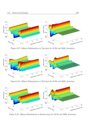
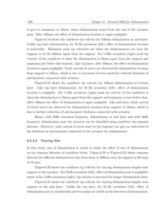
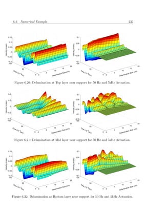
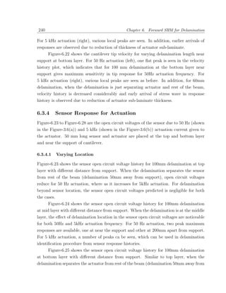
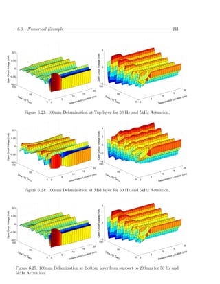
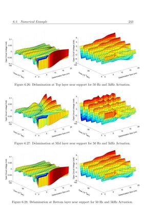
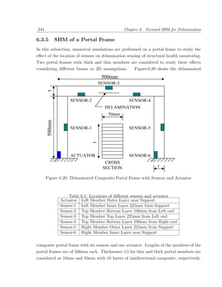
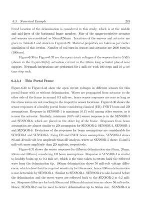
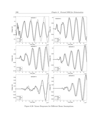
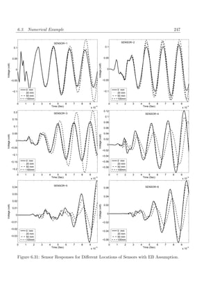
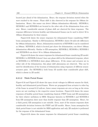
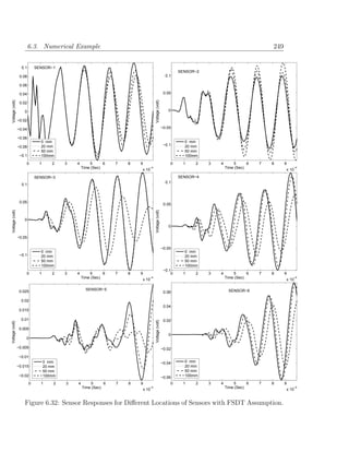
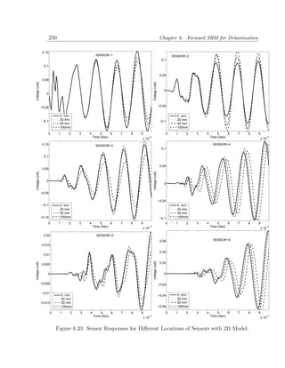
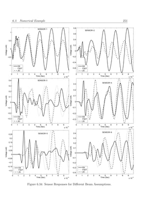
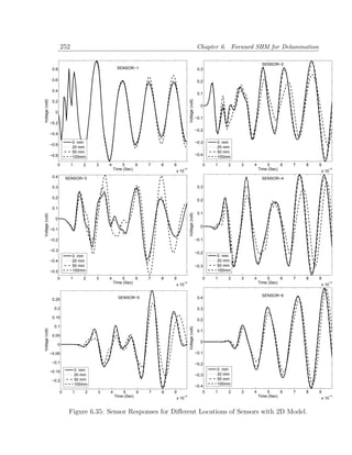
284. 256 Chapter 7. Structural Health Monitoring: Inverse Problem
the damage configuration of the structure, which can be used to get good assumption for
trial and error approach in the SHM.
In recent years, some researchers have applied ANN for structural damage detection
related applications [175, 215, 257, 294, 348, 350, 351, 358, 401, 402, 407, 416, 419, 418].
Much experience has been accumulated through these exploratory investigations. Lee
et al. [215] used the differences or the ratios of the mode shape components between
before and after damage for input to the neural networks. Faravelli and Pisano [117]
shown neural network approach to identify the damaged element of a multi-bay planar
truss structures. Angeles et al. [16] investigated nonlinear system identification of civil
structures using ANN. Xu [408] used ANN for sub-structural parametric identification of
post-earthquake damaged civil structures by the direct use of dynamic responses. Lee and
Lam [214] presented a neuro-fuzzy model for the diagnosis of structural damage. Rhim
and Lee [328] examined the feasibility of using ANN in conjunction with system identi-
fication techniques to detect the existence and to identify the characteristics of damage
in composite structures. Martin et al. [255] used artificial neural receptor system to
reduce the number of channel of data acquisition system for SHM. Zang et al. [421] pre-
sented structural damage detection from time domain data using independent component
analysis and ANN. Su and Ye [349] presented an online health monitoring technique for
in-service composite structures using 3D FEM, ANN and wavelet transform technique.
Ye et al. [416] reviewed performance of artificial intelligence techniques in functionalized
composite structures and as a specific case study, SHM technique was developed through
an ANN. Kao and Hung [175] detected structural damage using ANN from free vibration
responses. Su and Ye [348] trained multi-layer feed-forward, error-back propagation ANN
with the raw Lamb wave signals for SHM and validated the proposed method by locating
actual delamination and through-thickness holes in quasi-isotropic composite laminates.
Nyongesa et al. [294] proposed a technique combining conventional image analysis, ANN
classification and fuzzy logic inference to characterize shearograms for impact damage
detection.
In this chapter a methodology for automatic damage identification and localiza-
tion in composite structural components is presented using ANN. Responses for delam-
inated and healthy beam are computed using finite element analysis, which is discussed
in the earlier chapters. These responses and corresponding damage configurations are
used to train ANN as input and output of the network respectively. A feed-forward back-
propagation neural network is designed, trained, and to predict the delamination location

285. 7.2. SHM using Single ANN 257
using the structural response as inputs. Time domain response history is represented
by the responses of every time steps, which is high dimensional. Hence, dimension re-
duction technique is essential to use the response in the network. In Section-7.2, single
ANN is used to predict the damage properties after dimension reduction of time domain
responses. This dimension reduction looses the output uniqueness of the mapping from
response histories to damage properties. To overcome output uniqueness problem, output
space is partitioned and an ANN is trained for each partition. Finally, these trained ANNs
are coordinated with a committee machine, which is illustrated systematically in Section-
7.3. In Section-7.4, a hierarchical neural neural (HNN) is trained, validated and used for
mapping of the damage properties from response histories of the structure. Hundreds of
ANN is coordinated systematically with this HNN.
7.2 SHM using Single ANN
An artificial neural network (ANN) can learn the mapping between inputs and outputs
through a sample data set and determine the output of new data based on previous
knowledge. In this study, ability of identifying structural damage status for an ANN is
acquired through training the neural network using the known samples. Data obtained
from the magnetostrictive sensors described in earlier chapters, is used to train the network
to identify the delamination size of the composite laminate. The multi-layer feed-forward
network that is the most popular of the architectures currently available, is used. This is
a supervised learning procedure that attempts to minimize the error between the desired
and the predicted outputs. Standard logistic function y = 1/(1 + e−1.7159v ) is applied in
the hidden layer as activation function with linear output layer. This algorithm adjusts
the connection weights according to the back-propagated error computed between the
observed and the estimated results. The sample data set is separated into two parts,
one for training and the other for testing the network performance. The training stage
involves the network weights being adjusted until the network is able to satisfactory map
all data. Once trained, the network provides rapid mapping of a given input into the
desired output quantities. This, in turn, can be used to enhance the efficiency of the
mapping process.
Figure-7.1 shows the delaminated, 12 layered unidirectional composite cantilever
beam with actuator and sensor. Sensor response due to actuation is computed for the
beam as per the analysis shown in earlier chapters. In this section, numerical experiments

286. 258 Chapter 7. Structural Health Monitoring: Inverse Problem
Y
l w2 50 mm
d1
12
11
¡ ¡ ¡ ¡
0.15 X 12 = 1.8 mm
¡ ¡ ¡ ¡
¡
¡
¡
¡
10
¡
¡
¡
¡
A 9
SENSOR
y1
y
3
X 8
7
B 6
5
y2 ACTUATOR
4
3
2
1
w1 x3 d2
x1 x2
L= 50 mm X 10 = 500 mm
Figure 7.1: Delaminated composite beam with sensor and actuator.
are performed to identify the size of delamination using single ANN, where delamination
layer is known. As structural damage information is distributed in different vibration
modes, and vibration modes with high frequencies are generally more sensitive to small
damage, frequency of 5kHz is considered to excite the actuator (shown in Figure-3.6(b))
for better performance in the identification procedure. 51 different sample data sets are
numerically simulated for each layer of the delamination. These 51 cases include the
intact laminate and laminates with delamination of 50 different sizes (10 mm to 500 mm
with 10mm increment), where delaminations are started from support of the cantilever.
In order to identify the delamination length at each layer, one BP neural network with 10
inputs and 1 outputs are designed. Output node denotes the length of the delamination.
Every layer networks are trained by their corresponding 51 sample data. These samples
are for delamination in the corresponding layer or for healthy structure. Thus there are
eleven neural networks and these are trained for the corresponding layer to predict the size
of the delamination. Open circuit voltages of the sensor are high dimensional data. So,
first 5 peak values and their locations in time history are taken as input space of the ANN
mapping. Out of 11, two experiments are shown- one for top layer delamination and other
for mid layer. For each experiment two networks are trained with 10-5-1 (Figure-7.2) and
10-5-2-1 (Figure-7.3) architectures. All these four networks are trained up to one million
epochs and Figure-7.4 shows the training performance of the networks. With architecture
of 10-5-2-1, both the networks for top layer and mid layer are trained successfully. But
training performance of top layer networks with 10-5-1 architecture is relatively poor.

287. 7.2. SHM using Single ANN 259
Output
Output
Input
Input
Output Layer Hidden Layer Output Layer
Hidden Layer Hidden Layer
Input Layer Input Layer
Figure 7.2: ANN of 10-5-1 Architecture. Figure 7.3: ANN Architecture 10-5-2-1.
After training, networks are tested with different set of example for identification of
generalization capacity. 50 different sample data sets are numerically simulated for each
layer of the delamination for testing of these trained networks. These are for delamina-
tion of size 5 mm to 495 mm in 10mm increment. Corresponding testing performance of
trained networks are shown in Figure-7.5, where testing error gives an indication of the
generalization capacity of the trained network. For 10-5-1 architecture, both top and mid
layer networks are trained with satisfactory generalization capacity. Where as generaliza-
tion capacity of the mid layer network with 10-5-2-1 architecture is poor, which may be
due to overtraining of the network. However, it is showing that for both the architecture,
delamination is identified within 50mm accuracy by any of the trained networks.
7.2.1 Difficulties in Single ANN
Main problem of these trained 11 ANNs are, the delamination layer should be known
before, such that corresponding trained ANN will be used to predict the size of delami-
nation. This problem can be overcome by using single ANN with two output nodes one
for size and other for layer of the delamination. Combining the layer and the size of the
delamination, one single network is trained with two output node as per Figure-7.6. For
this experiment, one single ANN is tried to train with all these samples. However, this
network fails to train the samples, which is due to similar responses for different delamina-

288. 260 Chapter 7. Structural Health Monitoring: Inverse Problem
Mid Layer (ANN Arch: 10−5−1)
Top Layer (ANN Arch: 10−5−1)
−1
10
Error(%)
−2
10
1 2 3 4 5 6 7 8 9 10
Epoch 5
x 10
(a) 10-5-1 network architecture
Top Layer (ANN Arch: 10−5−2−1)
Mid Layer (ANN Arch: 10−5−2−1)
−1
10
Error(%)
−2
10
1 2 3 4 5 6 7 8 9 10
Epoch 5
x 10
(b) 10-5-2-1 network architecture
Figure 7.4: Training Performance of ANNs.

289. 7.2. SHM using Single ANN 261
500
Expected
450 Top Layer (ANN Arch: 10−5−1)
Mid Layer (ANN Arch: 10−5−1)
400
Delamination Length (mm)
350
300
250
200
150
100
50
0
0 10 20 30 40 50
Testing Sample
(a) 10-5-1 network architecture
500
Expected
450 Top Layer (ANN Arch: 10−5−2−1)
Mid Layer (ANN Arch: 10−5−2−1)
400
Delamination Length (mm)
350
300
250
200
150
100
50
0
0 10 20 30 40 50
Testing Sample
(b) 10-5-2-1 network architecture
Figure 7.5: Testing Performance of ANNs.

290. 262 Chapter 7. Structural Health Monitoring: Inverse Problem
tion configuration in dimensionally reduced input space. For training of networks, output
space uniqueness is essential requirement. Hence, to keep output uniqueness in the ANN
mapping, the output space is divided with different overlapped zones. Samples from these
zones are used to train a corresponding ANN with two output nodes. These ANNs are
coordinated with one committee machine, which is illustrated systematically in the next
section.
7.3 Committee Machine
Input
Committee Machine
Output
Input
Expert Expert Expert
Output Layer
Hidden Layer
Committee Machine
Input Layer
Output
Figure 7.6: ANN Architecture 10-5-2. Figure 7.7: Committee Machine.
It is perhaps impossible to combine simplicity and accuracy in a single model of
ANN. Here a simple model that uses hard decisions to partition the input space and
output space into a piecewise set of subspaces, with each subspace having its own expert
(Figure-7.7). Sizes of these subsets are such that the output uniqueness within a subset
is preserved as well as sufficient number of sample data is available to train and test
the network. Thus, for every subset, one expert is trained and tested taking sample
data from these subsets. Similar to the division of output space, input space can be
divided in different subsets on the basis of sensor, actuator and actuation combination.
However, as the input space subdivision is known a’priori, committee machine for input
space subdivision is not required. Single multi-layered perceptron (MLP) uses a black
box approach to globally fit a single function into the data, thereby losing insight into

291. 7.3. Committee Machine 263
the problem. Here computational simplicity is achieved by distributing the learning task
among a number of experts, which in turn divides the input space and output space into
a set of subspaces. The combination of experts is said to constitute a committee machine.
Basically, it fuses knowledge acquired by experts to arrive at an overall decision that is
supposedly superior to that attainable by any one of them acting alone.
7.3.1 Numerical Experiment using Committee Machine
Table 7.1: Performance of Committee Machine.
Exp- Span Span Layer Span Distance
erts Left Right Opinion Opinion
Sl (mm) Sr (mm) Ol (mm) Os (mm) D
1 0 50 -2.21 11.5 1.25
2 25 75 1.82 62.1 0.77
3 50 100 1.02 174 3.67
4 75 125 -2.13 92 0
5 100 150 -1.95 173 0.93
6 125 175 -1.61 168 0.55
7 150 200 8.64 172 22.77
8 175 225 -0.721 181 0
9 200 250 -2.63 238 1.88
10 225 275 -4.32 230 5.51
11 250 300 -0.444 314 0.35
12 275 325 -0.554 308 0
13 300 350 -1.01 322 0.07
14 325 375 0.203 334 0
15 350 400 -0.592 380 0
16 375 425 -0.595 380 0
17 400 450 0.600 458 0.19
18 425 475 0.0818 403 0.62
19 450 500 0.730 494 0
The beam is divided span wise in 19 different overlapped zones. For each zone, one
network (expert) is trained to predict the delamination layer as well as location. Table-
7.1 shows the span wise location in second and third columns (Sl , Sr ) for every expert.
Training and testing samples for corresponding experts are taken from their corresponding
zones. Figure-7.8 shows the training performance of different span wise experts. Networks
are trained up to 105 epoches. After that, the training errors become saturated. Figure-
7.9 shows the training performance of the first and fifth span wise experts. Both predicted

292. 264 Chapter 7. Structural Health Monitoring: Inverse Problem
0
Span Expert 1
10 Span Expert 2
Span Expert 3
Span Expert 4
Error(%)
−1
10
1 2 3 4 5 6 7 8 9 10
Epoch x 10
4
(a) Span Expert 1-4
0
Span Expert 5
10 Span Expert 6
Span Expert 7
Span Expert 8
Error(%)
−1
10
−2
10
1 2 3 4 5 6 7 8 9 10
Epoch x 10
4
(b) Span Expert 5-8
Figure 7.8: Training Performance of Different Span Experts.

293. 7.3. Committee Machine 265
−3
x 10
1 Predicted
Expected
0.8
0.6
0.4
Layer (mm)
0.2
0
−0.2
−0.4
−0.6
−0.8
−1
5 10 15 20 25 30 35 40 45 50 55
Span (mm)
(a) span expert 1
−3
x 10
1 Predicted
Expected
0.8
0.6
0.4
Layer (mm)
0.2
0
−0.2
−0.4
−0.6
−0.8
−1
100 110 120 130 140 150
Span (mm)
(b) span expert 5
Figure 7.9: Training Performance of span experts

294. 266 Chapter 7. Structural Health Monitoring: Inverse Problem
and expected layer and size of the delamination is shown in the figure. Layer wise errors
of the training samples are with in the thickness of the composite layer and span wise
errors are with in 5mm. Hence, this can be considered as well trained. After training,
each of the networks is used to test the generalization capacity as discussed in the earlier
section.
In identification face, time domain sensor outputs are fed into every networks to
get their opinions like, the location and size of the delaminations. These individual opin-
ions are fused by committee machine, which is illustrated in Table-7.1 through a simple
example. Table shows the performance of the committee machine for a delamination con-
figuration of (-0.6,380). In delamination configuration, first coordinate is for layer and
second is for delamination size. Prediction of the Expert-1 (which is trained with samples
from span of 0mm to 50mm) for this delamination configuration is (-2.21,115). Similarly,
every expert has given their opinions, which are shown in fourth and fifth columns in
the Table. As the networks are trained with the samples taken from their corresponding
zones, networks are experts for their corresponding zone only. Hence, the location of these
predicted opinions are checked with their corresponding experts zone first. For that, a
distance norm is used, where distance between their opinion and expertise zone is defined
as:
(Os − Sl )(Os − Sr ) (Ol − Lb )(Ol − Lt )
D = M ax , , 0 . (7.1)
(Sr − Sl )(Sr − Sl ) (Lt − Lb )(Lt − Lb )
Os and Ol are the opinion span and layer respectively. In the expression, top of the layer
(Lt ) and bottom of the layer (Lb ) are considered as +0.9mm and -0.9mm respectively.
If the distance is zero, the opinion is with in its expert location, and can be used as an
active expert for this particular delamination configuration.
In the Table-7.1, only expert-4, 8, 12, 14, 15, 16 and 19 are the active experts as
their opinions are with in their corresponding expert zones. However, only expert 15 and
16 gives mutually agreeable prediction and all other give mutually contradictory opinion.
Therefore, these noisy experts are removed from the active list and average opinion of the
expert 15 and 16 is used as prediction of the committee machine. Average of these opinion
is (-0.593,380), which is very close to original delamination configuration (-0.6,380).
When the number of active expert is quite large, finding of mutually agreeable
experts or removing of noisy expert is difficult manually. One systematic procedure to
remove such noisy experts is explained in Figure-7.10. All the active experts are plotted
according to their opinion in the figure. First, the mean of all these active expert’s opinion
is computed and shown in point ’A’ in the figure. Then furthest expert from this mean

295. 7.3. Committee Machine 267
500
Expert−19
450
400 Expert−16
Expert−15
Delamination Span (mm)
350 D
Expert−12 Expert−14
C
300
A
B
250
200
Expert−8
150
100 Expert−4
50
−6 −4 −2 0 2 4 6
Delamination Layer (m) −4
x 10
Figure 7.10: Removal of Noisy Expert.
(here Expert-19) is considered as noisy expert and excluded from the list of active expert.
After excluding this noisy expert, again mean is calculated among the rest of the active
experts, which is shown as point ’B’ in the Figure. In this way, gradually all the noisy
experts will be removed one by one and mean of the remaining active experts will move
from points ’A’-’B’-’C’-’D’ to the average opinion of expert-15 and 16.
7.3.2 Information Loss due to Dimension Reduction
Dimension of the time domain response is so large, it is not possible to use directly as
input node in the neural network. Moreover, values for some of the nodes are constant
for the entire training sample, which will create difficulty to train the network. As an
example, responses at time step zero are zero for every delamination configuration. One
approach of this problem is dimensional reduction of the responses, like, principle com-

296. 268 Chapter 7. Structural Health Monitoring: Inverse Problem
ponent analysis, independent component analysis, peak values or locations. However,
the information loss due to this dimension reduction may reduce the damage detection
capacity of the ANNs. This information loss can be compensated using more number of
dimension reduction procedure, rather than a single one, where probability of preservation
of the damage signature is more. Next section gives a systematic procedure to use more
than one dimension reduction in hierarchical Neural Network (HNN).
7.4 Hierarchical Neural Network (HNN)
With the common multi-layer neural network architectures, networks lack internal struc-
ture; as a consequence, it is very difficult to discern characteristics of the knowledge
acquired by a network in order to evaluate its reliability and applicability. Alternatively,
neural network architecture is presented, based on a hierarchical organization. By using
the hierarchical scheme, a complicated large-scale system is decomposed into a set of lower
order subsystems and a coordination process, and thus becomes tractable.
7.4.1 Five Stage HNN
A five-stage hierarchical neural network is designed by combining multi-layer perceptrons
for first stage and mixture-of-experts in the subsequent stages. The second stage mixture-
of-expert, ensembler network, learns to minimize the overtraining errors. The third stage
mixture-of-expert, validation network, learns to minimize the generalization errors. The
fourth stage mixture-of-expert, expert network, learns to minimize the error of network
due to loss of information for reduction of input space dimension, and finally, the fifth
stage committee machine choose the appropriate expert network from all expert networks.
The whole procedure is discussed as follows.
7.4.1.1 Neural Networks
In the first stage, multi-layer perceptrons are used to map dimensionally reduced sensor
response to damage space. Training and testing of a single multi-layer perceptron is
explained in Section-7.2 extensively.
7.4.1.2 Ensemble Network
Often artificial neural networks are prone to overtraining, where network trains the com-
putational and experimental noises. And there is no direct rule to draw the line between

297. 7.4. Hierarchical Neural Network (HNN) 269
well trained and overtrained for a set of training examples and network architecture.
One of the indirect ways to get a measure of overtraining of the network is Ensemble
Network. In ensemble network, a number of neural networks are trained with the same
training samples but with different initial conditions, learning rate, training algorithm,
network architecture and training sequence (for sequential learning). In training phase,
each network trains and generates training error for the training samples. On the basis of
these training errors, weightages of the trained neural network is determined, where less
training error gives more weightage of the neural network. In the execution phase, these
weightages are used to get weighted average of all neural networks output as the output
of ensemble network. From the distribution of the output of different neural networks
and their corresponding weightages, one measure of overtraining can be computed. If the
outputs of different neural network are close (at least for those have more weightages)
then networks are well trained otherwise it is overtrained. Every trained neural network
is tested through the test data set, which gives the testing errors as a measure of gener-
alization of the neural networks. These testing errors with the weightages of the neural
networks give the weighted average of testing error, as a measure of testing error of the
ensemble network. Next issue in the HNN is the generalization of the network using the
testing error of ensemble network.
7.4.1.3 Validation Network
As, every neural network within the ensemble network is trained with same training
sample; these neural networks need testing for generalization of the ensemble network. For
testing of network, sample data set is separated into two groups, one for training and other
for testing (validation). Different partitioning of sample data is explained in Figure-7.11.
After training of neural networks, with the training samples, the neural networks simulate
the testing sample and get the testing error. These testing errors with their weightages give
the measure of generalization of the ensemble network. However, every neural network in
the ensemble network is trained and tested through the same set of training data set and
testing data set respectively. To get a more general input-output mapping from a set of
sample data set, different division of training sample and testing sample is essential. This
can be done through a systematic manner using validation network. Validation Network
consists of some number of ensemble networks. These ensemble networks are trained
and tested with same sample data set with different partition for training data set and
testing data set as shown in Figure-7.11. However, every validation network is trained and

298. 270 Chapter 7. Structural Health Monitoring: Inverse Problem
10
Training Set Testing Set
9
Partition−11
Partition−10
8
Partition−9
Partition−8
7
Partition−7
Partition−6
6
Partition−5
Partition−4
5
Partition−3
Partition−2
4
Partition−1
Testing Set Training Set
3
Sample Data Set
2
1
Training Data Set Testing Data Set
0
0 1 2 3 4 5 6 7 8 9 10
Figure 7.11: Partition of Sample Set.
tested by a fixed set of sample data set, which comes from different dimension reduction
procedures.
7.4.1.4 Expert in HNN
In time domain structural health monitoring, time histories of the sensor outputs (open
circuit voltages) are the original input space for the input-output mapping. As explained
earlier, it is not possible to train the network taking full dimension of the original input
space (sensor output). To address this issue, different dimension reduction procedures
are available in the literature, which can reduce the dimension of the original input space
keeping main features of the high dimensional data. However, for structural health mon-
itoring, suitable dimension reduction procedure is not available, which will reduce the
dimension of the input space preserving the signature of damage from the high dimen-

299. 7.4. Hierarchical Neural Network (HNN) 271
sional sensor output. To overcome this problem, a number of reductions procedures are
taken to increase the chance of preserving the damage signature in the reduced input data
sets. This issue is taken care by a systematic manner in the fourth stage of the HNN.
Expert consists of a number of validation networks, which were trained and tested
through same output of a sample data set but with different lower dimensional input
of the data set. These different input data sets come from different dimension reduction
procedure of the original input set, which is high dimensional sensor output. Hence, every
expert is a mapping from sensor output to the damage properties of the structure and
performance of the expert depends on the performances of its validation networks, which
is trained through dimensionally reduced input sample set.
7.4.1.5 Committee Machine in HNN
Some times, due to this reduction procedure, the mapping looses the output uniqueness,
which is essential for the training of neural network. This problem was studied by parti-
tioning the input and output space into a piecewise set of subsets, with each subset having
its own expert. Committee machine is discussed extensively in earlier section (Section-
7.3) taking experts as a single neural network, which lacks information about the level of
confidence of the decisions.
7.4.2 Training Phase of HNN
In training phase, high dimensional samples (original sensor output) are fed to the expert,
which are within their expert zone. Every expert gives these samples to their subordi-
nates (validation networks), after assigned dimension reduction. The validation networks
then create different set of partition for training and testing samples and transfer these
partitions to the corresponding ensembler network. Similarly, every ensembler network
gives these training and testing samples to their subordinate, ANN network, for training
and testing of the networks. Thus, ANN gets their samples for training and testing of the
network from the original high dimensional sensor open circuit voltages. Training, testing
(validation) and execution (simulation) phase of the HNN is illustrated in Figure-7.12 and
discussed as follows:
7.4.2.1 Training of ANN
In training phase, every multilayer perceptrons (MLP) are trained with their correspond-
ing training samples. These training samples will give their training error as per the

300. 272 Chapter 7. Structural Health Monitoring: Inverse Problem
Sensor−actuator Mean Variance
configuration,
Actuation history
Committee Machine
Partitioning of input and Active(:)
output space
Sample set is fixed
Expert Expert Expert Opinion Opinion No of Zero
in original input space
Mean Variance Distance
Dimension reduction of input
space−PCA, ICA, peak
value, peak location Distance
Opinion
Sample set is fixed
Validator Validator Validator Validation
in reduced input
space Weight(:) Variance
Separation of Training
and validation set
Avarage
Training set and
Validation set is Ensembler Ensembler Ensembler ANN Validation ANN ANN
fixed Weight(:) Error Mean Variance
Generation of ANNs with
random architecture
and training
properties
ANN ANN ANN Training Validation ANN
Architecture Error Error Opinion
Momentum rate,
Learning rate, Algorithm, Sequence
Phases Training Validation Execution
Figure 7.12: Training, Validation and Execution of 5 stage HNN.
discussion in Section-1.4.6.1. Training error for ith ANN, Eti , is mean squire error of all
the samples used in training. Due to different network architectures, learning algorithms,
initial condition, learning rate, momentum rate and learning sequence, the ANNs will be
trained differently. This step will take more than 98% computation time of total training
of HNN.
7.4.2.2 Training of Ensembler Network
Relative training performances of ANN are stored in Ensembler network. Depending upon
the training error, every trained ANN under an ensembler network is associated with their

301. 7.4. Hierarchical Neural Network (HNN) 273
weightages. This ANN weightages (WA ) for k th ANN are computed as:
k
Na −1 Na
k 1
WA = Etk ⇒ k
WA = 1. (7.2)
i=1
Eti k=1
Where Na is the number of ANN under the ensembler.
This is the training phase of the hierarchical network. Training phase is limited
within ANN and ensembler network.
7.4.3 Testing Phase of HNN
As mentioned earlier, in testing phase, every ensembler network gives testing samples to
their subordinate ANN network taken from validation network.
7.4.3.1 Testing of ANN
Every trained ANNs are tested with their corresponding testing (validation) samples.
These testing samples will give their testing errors as per the discussion in Section-1.4.6.4.
Testing error for ith ANN, Ev , is mean squire error of all the samples used for testing.
i
7.4.3.2 Testing of Ensembler Network
Training weightages (WA ) and validation errors (Ev ) of all the subordinate ANNs are
considered to calculate average validation error (VE ) of an ensemble network. This average
validation error for ensembler network is considered as:
Na
k k
VE = Ev WA (7.3)
k=1
Where Na is the number of ANN under the ensembler.
7.4.3.3 Testing of Validation Network
Relative performance of ensembler networks under a validation network are calculated
from these average validation errors (VE ). Every validation networks calculate weighted
average validation error for ensemble networks. Thus, weighted average validation error
(WV ) of k th ensembler network is calculated as:
Nr −1 Nr
k k 1 k
WV = VE i
⇒ WV = 1. (7.4)
i=1
VE k=1

302. 274 Chapter 7. Structural Health Monitoring: Inverse Problem
Where, Nr is the number of ensembler networks under the validation network.
This is the testing phase of the hierarchical network. Testing phase is limited within
ANN, ensembler network and validation network.
7.4.4 Execution Phase of HNN
In execution phase, execution samples (high dimensional sensor output) are fed into every
expert to get their opinion and confidence. Similar to training phase, execution samples
reaches to ANN network after proper dimension reduction.
7.4.4.1 Execution of ANN
ANNs execute these samples and give their opinion (Oa ) as discussed in Section-1.4.6.5.
As different ANNs are trained differently, their opinion will also be different even for the
same execution sample.
7.4.4.2 Execution of Ensembler Network
Mean (Mr ) and variance (Vr ) of these opinions (Oa ) is calculated for the ensembler network
as:
N Na
1 a i 1
Mr = O , Vr = i
(Oa − Mr )2 (7.5)
Na i=1 a Na i=1
Here, Vr gives a measure of overtraining of the ANNs under that ensembler even without
using testing samples.
7.4.4.3 Execution of Validation Network
Information on validation network will be created by fusing ensembler level information.
In the execution phase of validation network, the weighted average validation error (WV ),
mean (Mr ) and variance (Vr ) of ensembler network are used. Opinion of validation network
(Ml ) is created by the mean of ensembler network (Mr ) and their corresponding weighted
average validation error (WV ) as:
Nr
k k
Ml = Mr WV (7.6)
k=1
Where, Nr is the number of ensembler networks under the validation network. Simi-
larly, variance of validation network (Vl ) is created from mean (Mr ) and variance (Vr ) of

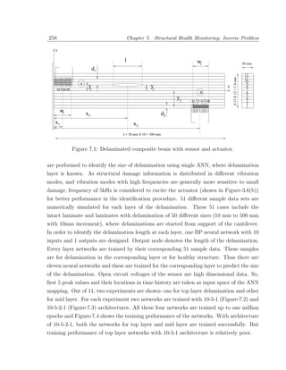
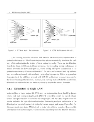
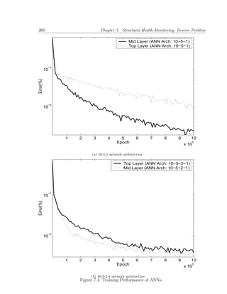
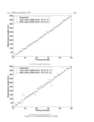
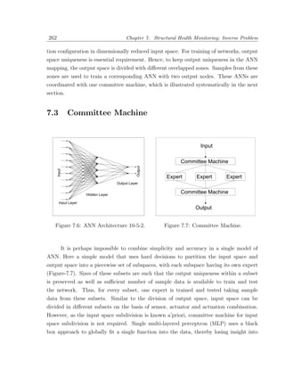
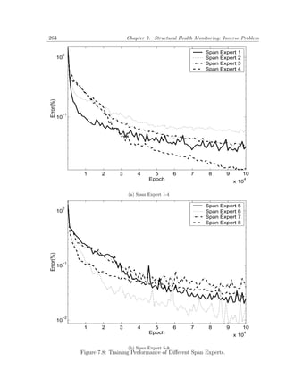
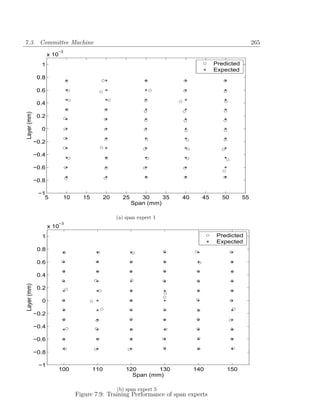
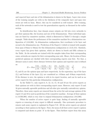
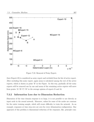
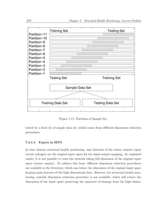
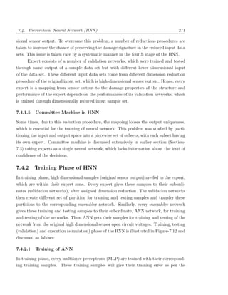
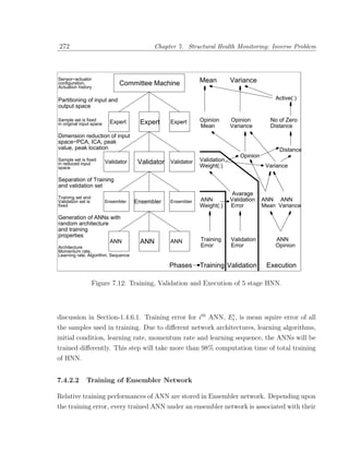
303. 7.4. Hierarchical Neural Network (HNN) 275
ensembler network with their weighted average validation error (WV ) as:
Nr
Vl = WV M ax (Mr − Vrk − Ml )2 ,
k k
(Mr + Vrk − Ml )2
k
(7.7)
k=1
Distance, D of the validation network is computed as per the Equation-(7.1) shown in
Section-7.3.1. If the opinion of validation network is with in the expertise zone of inherited
expert, and variance is with in their accepted limit, this validation network is considered
as active validation network.
As dimension reduction algorithm is different between different validation networks,
weightages (Wd ) for dimension reduction can be utilize to give more importance for better
dimension reductional algorithm.
7.4.4.4 Execution of Expert Network
Opinion (Ml ), variance (Vl ) and distance (D) of every validation network under every
expert are computed. For execution in the expert level, information of validation networks
are fused. First, the distance (D) for every validation networks are calculated and tagged
as active validation network if the distance is zero as per Section-7.3.1. Then the number
of active validation networks is counted under every expert.
7.4.4.5 Active Expert Network
Active experts are determined depending upon which expert has maximum number of
active validation network. If only one expert is active expert, weighted opinion and
weighted variance of all active validation networks under this expert are calculated, and
considered as the opinion (Mc ) and variance (Vc ) of the HNN. Where opinion (Mc ) of the
HNN is formulated as:
  −1
Mc =  Mlj Wd  
j
Wd 
j
(7.8)
[j∈Nl ] [j∈Nl ]
and variance (Vc ) of the HNN is formulated as:
 −1
2
Vc = j
(Wd ) M ax (Mlj − Vlj − Mc )2 , (Mlj + Vlj − Mc )2  Wd 
j
(7.9)
[j∈Nl ] [j∈Nl ]
j
where, Nl is the set of active validation network under the same expert and Wd is the
weightage of the j th dimensional reductional algorithm.

304. 276 Chapter 7. Structural Health Monitoring: Inverse Problem
If more than one active expert is available, first, Equation-(7.8) and Equation-(7.9)
are used to get individual expert opinion (Mx ) and variance (Vx ), and then committee
machine is used to remove the noisy experts as per Section-7.3 to get the opinion (Mc )
and confidence (Vc ) of HNN.
7.4.5 Numerical Study of Five Stage Hierarchical ANN
−4
x 10
2.5
HNN identification
2 Expected Value
1.5
Delamination Layer(mm)
1
0.5
0
−0.5
−1
−1.5
−2
−2.5
200 250 300 350 400
Delamination Span(mm)
Figure 7.13: Performance of HNN.
In this study, 5 kHz sinusoidal current is considered in the actuation coil as per
earlier section. The vibration responses of 551 different cases are numerically simulated.
These 551 cases include the intact laminate, laminates with delamination damage at

305. 7.5. Summary 277
different layers and of 50 different delamination sizes (10 mm to 500 mm) at each layer.
Vibration responses of higher dimension for a given delamination, is preprocessed for
dimension reduction in the input space of the neural network. Here for simplicity first ten
peak values and their location of the sensor open circuit voltage and their time integrals are
taken as the input space of the four type of validation neural network. Every validation
network consists of four ensemble networks. These ensemble networks are trained and
tested by same sample data set but with different random partitioning between training
and testing data sets. Hence, every ensemble network is trained and tested by a fixed
set of training and testing data sets respectively. In order to identify the delamination
length and layer, a simple ANN neural network with 10 inputs and 2 outputs is designed.
One hidden layer of node strength 5 is considered in the network. The architecture of the
neural network is 10-5-2 and shown in Figure-7.6.
Output space is divided with nineteen span wise overlapped zone as discussed earlier
Section-7.3. Thus there are nineteen experts to predict the size and location of the
delamination. Every expert is trained by the sample data within their expertise locations.
These samples are for the delamination in the corresponding location. A number of
delamination identification is performed using proposed Hierarchical neural network and
shown in the Figure-7.13, where delamination layers as well as size of the delamination is
predicted efficiently.
7.5 Summary
The present chapter has shown the feasibility of using time domain magnetostrictive
sensor response for damage detection in composite beam numerically, with the mapping
features of the artificial neural networks (ANN). First, a single neural network is used to
identify the size of the delamination, where the layer of the delamination is known. Next,
the committee machine is used to coordinate different networks, which are exclusively
trained for different overlapped zones in the composite beam to identify both the layer
and size of the delamination simultaneously. And finally, one five stage hierarchical neural
network is trained to systematically consider different issues for mapping with ANN, like
overtraining, loss of output uniqueness and damage signature due to dimension reduction
of the sensor response and level of confidence in the prediction of the network. The present
numerical examples prove that using the artificial neural network, identification of size
and location of delamination is feasible.

306. Chapter 8
Summary and Future Scope of
Research
The work presented in the last six chapters gives a comprehensive account of the current
status of the structural health monitoring (SHM) of composite structures using magne-
tostrictive sensor and actuator. In this chapter, an overview of the whole thesis is provided
along with an outline of the possible future works on SHM using magnetostrictive sensors
and actuators.
The main objective of this thesis was to develop the necessary numerical tools for
the structural health monitoring of composite structures. The focus here was in the use
of magnetostrictive material as sensor/actuator materials to trigger the required inter-
rogatory signal for the active SHM. Hence, the first part of this thesis was developed to
the numerical material characterization of the highly nonlinear magnetostrictive material,
Terfenol-D. This was dealt in Chapter-2, where in two approaches, namely the polynomial
approach and ANN were employed to completely characterize both sensing and actuation
law of the magnetostrictive material. It is seen that ANN approach gives 5 to 10 times
more accurate prediction than polynomial approach. The necessary features of coupled
and uncoupled model were highlighted in this chapter.
Chapter-3 discussed a new finite element formulation for structures with in-built
magnetostrictive patches that can also handle coupled analysis. Here, both magnetic and
mechanical degrees are considered as unknown degrees of freedom. The developed FE
model can handle smart patches embedded in the laminates, which are required to induce
actuation strains on the application of magnetic field. This changes the state of stress in
the sensing patch and hence the magnetic flux density through the enclosed magnetic coil
changes, resulting in a voltage across the sensing coil. These developed elements are used
to study the effect of coupling in the overall performance of the structure. The response
278

307. 279
difference between healthy and damaged structure is 2 to 5 times less sensitive than the
difference between coupled and uncoupled formulations. Comparing the error due to
uncoupled analysis with the sensitivity of the damage in structural response, it is shown
that the coupled analysis is very essential for structural health monitoring applications.
In Chapter-4 of the thesis, two super convergent beam elements with embedded
magnetostrictive patches were developed, one for Euler-Bernoulli beam and the other for
first order shear deformable beam. As a result, in most cases, only a single element is ade-
quate to capture the superconvergent static behavior irrespective of boundary conditions
and ply-stacking configuration. For static tip deflection, single such element is within
0.05 to 0.4% error from 2D FE results. Also, its superconvergent behavior for vibration
and wave propagation problem was demonstrated. Dynamic Responses and natural fre-
quencies with 10 superconvergent elements shows better results than with 20 conventional
elements. Next, these developed elements were used for material property identification
from sensor response with the help of mapping properties of artificial neural network and
shown that it is identifying within 1% accuracy.
Chapter-5 deals with a new higher order spectral element, which is developed for
wave propagation analysis of a magnetostrictive embedded composite beam in the pres-
ence of thermal, magnetic and mechanical loading. The element is based on Higher
order Shear deformation with Higher order Poisson’s contraction Theory (HSPT) that
is, the formulated element can handle nth order shear deformation and nth order Pois-
son’s contraction. Numerical examples are directed towards highlighting the effect of the
requirement of higher order theories on the structural and magnetic responses. For exci-
tation of 100kHz, third order contraction and fourth order shear deformable assumption
is required. The spectrum and the dispersion relations were studied in detail. Developed
elements were then used for force identification from the sensor response of the struc-
ture and shown that 4 mili-sec sensor response can reconstruct 25 kHz broadband force
excitation exactly.
Delamination is the most important mode of damage on composite laminate. In
Chapter-6, numerical simulation were carried out for a delaminated composite laminate
with or without magnetostrictive patches as sensors and actuators using anhysteretic,
coupled, linear properties of magnetostrictive materials. Effect of delamination on the
cantilever tip velocity and the sensor open circuit voltages are studied. Single and multiple
delaminations are considered with tip vertical impact load and biased sinusoidal current
in the actuator coil. Amplitudes of reflections for 100mm delamination is similar to the

308. 280 Chapter 8. Summary and Future Scope of Research
reflection from the support of healthy beam, which can be identified easily. Although, the
reflection for 10mm single delamination is undetectable, 10 mm symmetric delaminations
can be identified. Next, the sensitivities of the delamination on the location of the sensors
were studied for a portal frame and shown that the sensor near the delamination have
maximum sensitivity.
Chapter-7 illustrated a methodology for automatic damage identification and local-
ization in composite structural components using various ANN. Responses for delaminated
and healthy beam was calculated as per Chapter-6. These responses and the correspond-
ing damage configurations were used to train ANN as input and output of the network,
respectively. The Feed-forward back-propagation neural network, the committee machine
and the Hierarchical Neural Network (HNN) were designed, trained, tested and to predict
the delamination location using the structural response as inputs. Single ANN can iden-
tify length of the delamination with in 50mm accuracy. Committee machine can predict
delaminated layer exactly. Five stage HNN shows quite accurate identification in both
location and length the of delamination, simultaneously.
8.1 Contribution of the Thesis
The main contribution of this thesis is outlined as:
1. One, two and three dimensional finite element formulation for both coupled and un-
coupled analysis was developed using developed constitutive relationships of mag-
netostrictive materials.
2. Developed superconvergent finite element formulation for analysis of beam with
magnetostrictive materials.
3. Higher order spectral finite elements are formulated and developed considering nth
order of shear and contraction effects.
4. Force and material property identification from the magnetostrictive sensor response
procedure were established.
5. The effects of the delamination and the multiple delaminations on the structural
and magnetostrictive sensor responses were studied due to known force actuation
and current excitation in the magnetostrictive actuator embedded in the composite
structure.

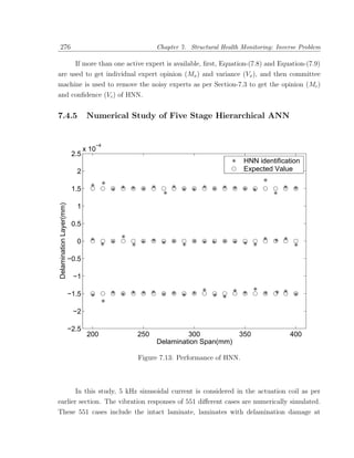
309. 8.1. Contribution of the Thesis 281
Table 8.1: Comparison with existing state-of-the-art
Present Study State-of-the-art
Degrees of freedom Both mechanical and Mechanical [326, 216]
in FE Formulation smart dof, Coupled dof, Uncoupled
Elements with Rod, Beam, Plate, Beam [326],
magnetostrictive 3D and Plane Plate [216],
sensor/actuator stress/strain Uncoupled
Modelling Equivalent Layer wise plate theory [29],
of single layer, Spectral [284, 285],
delamination Beam and Plate
Superconvergent Magnetostrictive FGM [63], Higher order beam [114]
Element actuator/sensor Thin walled composite beam [268]
th
Spectral Element n order Rod [109], Elementary beam [110, 111],
formulation (Poisson’s and Timoshenko beam [140],
shear) Beam with Poisson’s contraction [64]
magnetostrictive FGM beam and plate [59],
sensor/actuator Composite beam [249] tube [250]
Force Magnetostrictive Layered system [330], PZT [82],
Identification sensor response, Velocity [159], Wavelet [271],
Technique FFT based Spectral Greens’s function [373],
finite element Kalman Filter [239],
Multiple location [405],
ANN [228], Moving force [211],
FGM [61], Least square [413],
Delamination Time domain Natural frequency [127, 213, 251, 371],
Study study with Lamb wave [332, 350],
Single and Layer wise delamination [29, 72, 212],
multiple Damage spectral element [284, 285],
delamination, multiple delamination [191, 247],
magnetostrictive Fiber optic [234, 410]
sensor/actuator
In-situ sensor/material Magnetostrictive FGM beam and plate [59]
property identification sensor response, ANN
Geometric Delamination Mode shape [158], Modal damping [176],
Inverse study using Curvature mode shape [143],
problem ANN, Crack [125, 206, 287],
Committee machine, Fuzzy logic [359],
Five stage Dynamic residual force [126],
hierarchical Prestress concrete [243],
neural Embedded Flaw [319],
network ANN [328, 350], PZT [352, 391]

310. 282 Chapter 8. Summary and Future Scope of Research
6. Location of the sensors on the structural response were studied for a critical location
of delamination in a composite portal frame.
7. Developed five stage hierarchical neural network for automatic damage detection
from measured responses.
8.1.1 Limitation of the Approach
Weights of magnetostrictive sensor/actuator with corresponding coils are high. Hence,
SHM in this approach in aerospace application may be limited. For an array, the density
of sensors certainly depends on the particular physical mechanism of the sensing material.
For example, because of the prestress requirement, and because coils are usually required
to generate magnetic fields, magnetostrictive actuators are generally physically more cum-
bersome to construct than piezoceramic actuators. Therefore, for array applications with
high sensor/actuator density, piezoceramics or piezopolymers would be preferred. Al-
though such strains are larger than those achievable in piezoceramic materials, optimum
performance requires that a stress be applied to the magnetostrictive prior to actuation,
which renders certain applications impractical.
8.2 Future Scope of Research
This section will highlight the direction where the research can be extended.
• Multi-scale modelling of magnetostrictive patches is essential to get the exact fea-
tures of the patches. Two different scales one for the macro features and others for
the micro features can be used in the analysis.
• In Chapter-2, the thesis studied the anhysteretic coupled and uncoupled constitutive
relationships. In future, hysteretic coupled and uncoupled model of magnetostrictive
materials can be studied, which can be used in structural application.
• More recently, mesh less finite element is gaining popularity among the finite element
community. Mesh less formulation with magnetostrictive sensor and actuator can
be studied.
• As the magneto-mechanical coupling coefficient of magnetostrictive material is highly
nonlinear and hysteretic, some nonlinear finite element analysis can be done.

311. 8.2. Future Scope of Research 283
• In Chapter-4 super convergent formulation of only Euler-Bernoulli and FSDT were
studied, this can be extend to higher order beam formulation also.
• In Chapter-5 spectral analysis is done through FFT, which has in-built difficulties
to give boundary condition in time. These difficulties can be removed using some
time-frequency transformation like wavelet transformation.
• Structural response in frequency domain for delaminated beam requires the formu-
lation and development of damaged spectral element with magnetostrictive sensor
and actuator in-built. In addition, thus developed spectral element can be compared
with superconvergent element with same case study of SHM.
• Recently modelling carbon nano-tube (CNT) is gaining importance due to their su-
perb electrical and mechanical properties. Dynamic responses on single wall CNT
for Tera Hz loading is studied by many researchers in both spectral and as well as
conventional finite element. Research in modelling of multi wall CNT is still in prim-
itive stage due to its radial Van der Waals forces (a particular class of intermolecular
forces) and breathing mode of vibration. Present higher order spectral element can
be extended to semi-infinite curve plate, which can model multi wall CNT easily
with a pair of cylindrical elements. Researchers are already trying to insert different
chemicals inside the carbon nano-tube. Similarly, if any magnetostrictive material
is inserted inside CNT, it can be used as non contact nano sensor or actuator. This
nano sensor can be modelled using the above approach.
• In this thesis, other than delamination, simplified modelling of matrix cracking and
fiber breakage is addressed. More sophisticated models are possible to be formulated
under this SHM environment.
• Numerical study of optimum location of sensor is performed for time domain anal-
ysis. Study of optimum location of sensor in other domain, like frequency domain
or wavelet domain may give more information on SHM study.
• Gradually SHM community is moving from smart structural era to wireless com-
munication with MEMs and Nano sensors era. The main advantages and features
of this wareless based SHM will be:
– Multiple and heterogeneous sensors and actuator integration

312. 284 Chapter 8. Summary and Future Scope of Research
– Optimal location of actuator and excitation frequency selection
– Wireless communication with MEMs and Nano sensors
– Optimization of noise to signal ratio
– Million Wireless MEMS Communication hub with billion Nano-sensor in each
structural component
– Hierarchical decomposition of sensor networks
– Software and Hardware development
– Simultaneous SHM with vibration suppression
Thus in this line, the magnetostrictive thinfilm can be used as MEMS and modelled
with existing formulation. Similarly magnetostrictive-nano sensor can also be made
and used in SHM.
• Recent interest of artificial neural network is moving from multi layer perceptron
to support vector mechine (SVM), which can be used for both identification and
estimation (support vector regression) of the damages.
• As every analysis in finite element is computationally costly, Response Surface
Method (RSM) can be used to map the response features of the structure from
damage configuration. For this, some initial finite element simulation is required for
a particular set of damage configuration dictated by Design Of Experiment (DOE).
Once the response surface is generated, Evolutionary Algorithm (EA) can be used
to search the damage configuration without doing any further finite element simu-
lation.
• Fuzzy Logic (FL) is one of the powerful tool in soft computing, which can be used
independently or combined with ANN or EA for SHM.

313. Appendix A
Euler-Bernoulli Beam
¯
[N (x)] is the shape function matrix for mechanical degrees of freedom and are expressed
as
2 2
¯ x ¯12 = −2 xβe + 2 βe x , ¯13 = − xβe + βe x ,
N11 = 1 − , N N
L L2 L3 L L2
2
¯ x ¯ xβe βe x ¯ xβe βe x2
N14 = , N15 = 2 2 − 2 3 , N16 = − + 2 ,
L L L L L
¯ ¯ x2 x3 ¯ x2 x3
N21 = 0, N22 = 1 − 3 2 + 2 3 , N23 = x − 2 + 2,
L L L L
¯ ¯ x2 x3 ¯ x2 x3
N24 = 0, N25 = 3 2 − 2 3 , N26 = − + 2 , .
L L L L
¯ ¯ x x2 ¯ x x2
N31 = 0, N32 = −6 2 + 6 3 , N33 = 1 − 4 + 3 2 , .
L L L L
¯ ¯ x x2 ¯ x x2
N34 = 0, N35 = 6 2 − 6 3 , N36 = −2 + 3 2 . .
L L L L
[K] is the element stiffness matrix. {RT } and {RI } are element load vector coefficient
due to temperature rise and current actuation respectively.
A11 B11 A11 B11
K11 = , K13 = − , K14 = − , K16 = ,
L L L L
γ + 9 D11 γ + 9 D11 γ + 9 D11
K22 = 4/3 , K23 = 2/3 , K25 = −4/3 ,
L3 L2 L3
285

314. 286 Appendix A. Euler-Bernoulli Beam
γ + 9 D11 γ + 12 D11 B11
K26 = 2/3 , K33 = 1/3 , K34 = ,
L2 L L
γ + 9 D11 γ + 6 D11
K35 = −2/3 , K36 = 1/3 ,
L2 L
A11 B11 γ + 9 D11
K44 = , K46 = − , K55 = 4/3 ,
L L L3
γ + 9 D11 γ + 12 D11
K56 = −2/3 , K66 = 1/3 .
L2 L
       
−Ae r
11p Aα
11 0 Aα
11
       
 0   0   0   0 
       
 e   α     α 
 rB11p   −B11   0   −B11 
{R} =   Inp +   (∆T ); {RU } =   Inp +   (∆T ).
 Ae r   −Aα   0   −Aα 
p  11p   11     11 
       
 0   0   
0   0 
      
e α α
−rB11p B11 0 B11
Where r is ratio between two permeabilities (µσ /µ ) and γ = βe A11 + 6βe B11 = 9βe B11 .
2
The nonzero elements of the mass matrix are
M11 = 1/3 LI0 , M12 = −1/6 I0 βe + 1/2 I1 , M13 = −1/12 LI0 βe − 1/12 LI1 ,
M14 = 1/6 LI0 , M15 = 1/6 I0 βe − 1/2 I1 , M16 = −1/12 LI0 βe + 1/12 LI1 ,
1 39 L2 I0 + 14 I0 βe 2 − 84 I1 βe + 126 I2
M22 = ,
105 L
11 2 7
M23 = L I0 + 1/15 I0 βe 2 − I1 βe + 1/10 I2 ,
210 30
1 −27 L2 I0 + 28 I0 βe 2 − 168 I1 βe + 252 I2
M24 = −1/6 I0 βe + 1/2 I1 , M25 =− ,
210 L
13 2 7
M26 = − L I0 + 1/15 I0 βe 2 − I1 βe + 1/10 I2 ,
420 30

315. 287
1
M33 = L 2 L2 I0 + 7 I0 βe 2 − 7 I1 βe + 28 I2 , M34 = −1/12 LI0 βe + 1/12 LI1 ,
210
13 2 7
M35 = L I0 − 1/15 I0 βe 2 + I1 βe − 1/10 I2 , .
420 30
1
M36 = L −3 L2 I0 + 14 I0 βe 2 − 14 I1 βe − 14 I2 , .
420
M44 = 1/3 LI0 , M45 = 1/6 I0 βe − 1/2 I1 , M46 = −1/12 LI0 βe − 1/12 LI1 ,
1 39 L2 I0 + 14 I0 βe 2 − 84 I1 βe + 126 I2
M55 = , .
105 L
11 2 7
M56 = − L I0 − 1/15 I0 βe 2 + I1 βe − 1/10 I2 , .
210 30
1
M66 = L 2 L2 I0 + 7 I0 βe 2 − 7 I1 βe + 28 I2 . .
210

316. Appendix B
Timoshenko Beam
Matrices for superconvergent Timoshenko beam element can be calculated considering α
and βf as:
A55 B11 A11 A55
α= , βf = . (B.1)
(D11 A11 − B11 B11 ) (A11 D11 − B11 B11 )
Shape function matrix for superconvergent Timoshenko beam element is given by
¯ x ¯ xα x2 α
N11 = 1 − , N12 = −6 +6 ,
L 12 + L2 βf L (12 + L2 βf )
¯ xLα x2 α (L2 βf + 6) ¯ x
N13 = −3 − 1/2 + 1/2 x2 α, N14 = ,
12 + L2 βf 12 + L2 βf L
¯ xα x2 α ¯ xLα x2 α
N15 = 6 −6 , N16 = −3 +3 ,
12 + L2 βf L (12 + L2 βf ) 12 + L2 βf 12 + L2 βf
¯ ¯ x − 1/6 x3 βf x2 β f
N21 = 0, N22 = 1 − 12 −3 ,
L (12 + L2 βf ) 12 + L2 βf
¯ (x − 1/6 x3 βf ) (L2 βf + 6) x2 (3 + L2 βf ) ¯
N23 = + 1/6 x3 βf − 2 , N24 = 0,
12 + L2 βf L (12 + L2 βf )
¯ x − 1/6 x3 βf x2 βf ¯ x − 1/6 x3 βf x2 (−6 + L2 βf )
N25 = 12 +3 , N26 = −6 − ,
L (12 + L2 βf ) 12 + L2 βf 12 + L2 βf L (12 + L2 βf )
¯ ¯ x2 β f xβf
N31 = 0, N32 = 6 2β )
−6 ,
L (12 + L f 12 + L2 βf
288

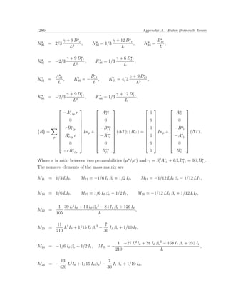
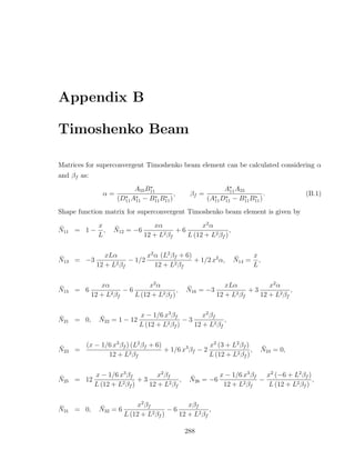
317. 289
¯ x2 βf (L2 βf + 6) x (3 + L2 βf ) ¯
N33 = 1 − 1/2 + 1/2 x2 βf − 4 , N34 = 0,
12 + L2 βf L (12 + L2 βf )
¯ x2 βf xβf ¯ x2 β f x (−6 + L2 βf )
N35 = −6 2β )
+6 , N36 = 3 −2 ,
L (12 + L f 12 + L2 βf 12 + L2 βf L (12 + L2 βf )
Nonzero entries of stiffness matrix. [K ] of Timoshenko beam is given by:
A11 B11 A11 B11
K11 = , K12 = 0, K13 = − , K14 = − , K15 = 0, K16 = ,
L L L L
A55 ψ A55 ψ
K22 = 12 , K23 = 6 A55 ψ, K24 = 0, K25 = −12 , K26 = 6 A55 ψ,
L L
D11 + 3 L2 ψ A55 B11 −D11 + 3 L2 ψ A55
K33 = , K34 = , K35 = −6 A55 ψ, K36 = ,
L L L
A11 B11 A55 ψ
K44 = , K45 = 0, K46 = − , K55 = 12 , K56 = −6 A55 ψ,
L L L
D11 + 3 L2 ψ A55
K66 = .
L
where ψ = 1/(12 + L2 βf ). Nonzero entries of mass matrix [M ] of a Timoshenko beam is
given by
M11 = 1/3 LI0 , M12 = −1/2 I0 L2 α ψ + 1/2 I1 − 6 I1 ψ, .
M13 = −1/12 L 3 I0 L2 α ψ + I1 + 36 I1 ψ , M14 = 1/6 LI0 ,
M15 = 1/2 I0 L2 α ψ − 1/2 I1 + 6 I1 ψ, M16 = −1/12 L 3 I0 L2 α ψ − I1 + 36 I1 ψ ,
Lψ 2
M22 = (13 βf 2 I0 L4 + 42 α2 I0 L2 + 294 βf I0 L2 + 1680 I0 − 84 βf α I1 L2
35
+42 βf 2 I2 L2 ),
11 11 12 7
M23 = I0 L2 − I0 L2 ψ + I0 ψ 2 L2 + 3/5 α2 I0 L4 ψ 2 − α I1 ψ L2
210 70 35 10
72 42 432
+ α I1 ψ 2 L2 + 1/10 I2 − I2 ψ + I2 ψ 2 , .
5 5 5

318. 290 Appendix B. Timoshenko Beam
M24 = −1/2 I0 L2 α ψ + 1/2 I1 − 6 I1 ψ, .
3Lψ 2
M25 = − (−3 βf 2 I0 L4 + 28 α2 I0 L2
70
−84 βf I0 L2 − 560 I0 − 56 βf α I1 L2 + 28 βf 2 I2 L2 ),
72 42 432 7
M26 = 3/5 α2 I0 L4 ψ 2 + α I1 ψ 2 L2 − I2 ψ + I2 ψ 2 − α I1 ψ L2
5 5 5 10
11 12 13
− I0 L2 ψ + I0 ψ 2 L2 + 1/10 I2 − I0 L 2 ,
70 35 420
1 6
M33 = I0 L3 − 1/35 I0 L3 ψ + I0 ψ 2 L3 + 3/10 α2 I0 L5 ψ 2 − 1/10 α I1 ψ L3
105 35
36 216
+ α I1 ψ 2 L3 + 2/15 I2 L − 6/5 I2 L ψ + I2 ψ 2 L,
5 5
M34 = −1/12 L 3 I0 L2 α ψ − I1 + 36 I1 ψ , .
72 42 432 7
M35 = −3/5 α2 I0 L4 ψ 2 − α I1 ψ 2 L 2 + I2 ψ − I2 ψ 2 + α I1 ψ L2
5 5 5 10
11 12 13
+ I0 L 2 ψ − I0 ψ 2 L2 − 1/10 I2 + I0 L 2 ,
70 35 420
1 6
M36 = − I0 L3 − 1/35 I0 L3 ψ + I0 ψ 2 L3 + 3/10 α2 I0 L5 ψ 2 − 1/10 α I1 ψ L3
140 35
36 2 3 216
+ α I1 ψ L − 1/30 I2 L − 6/5 I2 ψL + I2 ψ 2 L,
5 5
M44 = 1/3 LI0 , M45 = 1/2 I0 L2 α ψ − 1/2 I1 + 6 I1 ψ,
M46 = −1/12 L 3 I0 L2 α ψ + I1 + 36 I1 ψ , .
M55 = 1/35 L(13 βf 2 I0 L4 + 42 α2 I0 L2 + 294 βf I0 L2 + 1680 I0
−84 βf α I1 L2 + 42 βf 2 I2 L2 )ψ 2 , .
11 11 12 7
M56 = − I0 L2 + I0 L2 ψ − I0 ψ 2 L2 − 3/5 α2 I0 L4 ψ 2 + α I1 ψ L 2 ,
210 70 35 10
72 42 432
− α I1 ψ 2 L2 − 1/10 I2 + I2 ψ − I2 ψ 2 ,
5 5 5

319. 291
1
M66 = βf 2 I0 L7 ψ 2 + 1/5 I0 βf L5 ψ 2 + 3/10 I0 L5 α2 ψ 2
105
+6/5 I0 L3 ψ 2 − 1/10 βf α I1 L5 ψ 2
+6 α I1 L3 ψ 2 + 2/15 βf 2 L5 I2 ψ 2 + 2 I2 βf L3 ψ 2 + 48 I2 Lψ 2 .
The elements of force vector for a Timoshenko beam is given by
       
−Ae r11p Aα11 0 Aα
11
       
 0   0   0   0 
       
 e   α     α 
 rB11p   −B11   0   −B11 
{R} =   Inp +   (∆T ); {RU } =   Inp +   (∆T ).
 e   −Aα   0   −Aα 
p  A11p r   11     11 
       
 0   0   0   0 
       
e α α
−rB11p B11 0 B11
Where r is ratio between two permeabilities.

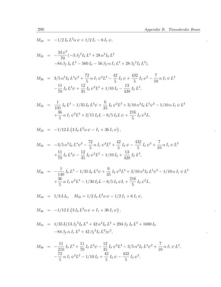
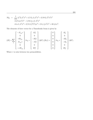
320. Appendix C
Higher Order Theories
Elements of stiffness [K], coupling stiffness [K m ] and mass [M ] matrices, are written as
1 [0] 1 [i] 1 [i]
Ku1 u1 = A ; Ku1 ui1 = A ; Ku1 w1 = 0; Ku1 wi1 = − iA13 ;
L 11 L 11 2
1 [0] 1 [i] 1 [i]
Ku1 u2 = − A11 ; Ku1 ui2 = − A11 ; Ku1 w2 = 0; Ku1 wi2 = − iA13 ;
L L 2
1 [i+m−2] 2 [i+m] i [i−1] 1 [i]
Kui1 um1 = imA55 L + 3A11 ; Kui1 w1 = − A55 ; Kui1 u2 = − A11 ;
3L 2 L
1 [i+m−1] [i+m−1] 1 [i+m−2] 2 [i+m]
Kui1 wm1 = − mA13 + iA55 ; Kui1 um2 = imA55 L − 6A11 ;
2 6L
i [i−1] 1 [i+m−1] [i+m−1] 1 [0]
Kui1 w2 = A ; Kui1 wm2 = −mA13 + iA55 ; Kw1 w1 = A ;
2 55 2 L 55
1 [i] i [i−1] 1 [0] 1 [i]
Kw1 wi1 = A55 ; Kw1 u2 = 0; Kw1 ui2 = − A55 ; Kw1 w2 = − A55 ; Kw1 wi2 = − A55 ;
L 2 L L
1 [i+m−2] 2 [i+m] 1 [i+m−1] [i+m−1]
Kwi1 wm1 = imA33 L + 3A55 ; Kwi1 um2 = mA13 − iA55 ;
3L 2
1 [i] 1 [i] 1 [i+m−2] 2 [i+m]
Kwi1 u2 = iA ; Kwi1 w2 = − A55 ; Kwi1 wm2 = imA33 L − 6A55 ;
2 13 L 6L
1 [0] 1 [i] 1 [i] i [i−1]
Ku2 u2 = A11 ; Ku2 ui2 = A11 ; Ku2 w2 = 0; Ku2 wi2 = iA13 ; Kui2 w2 = A55 ;
L L 2 2
292

321. 293
1 [i+m−2] 2 [i+m] 1 [i+m−1] [i+m−1]
Kui2 um2 = 2imA55 L + 6A11 ; Kui2 wm2 = mA13 + iA55 ;
6L 2
1 [0] 1 [i] 1 [i+m−2] 2 [i+m]
Kw2 w2 = A ; Kw2 wi2 = A ; Kwi2 wm2 = imA33 L + 6A55 ;
L 55 L 55 6L
m 1 1 [0] [0] m 1 1 [0] [i] i [0] [i−1]
Ku1 u1 = A A ; Ku1 ui1 = A11e A11e − A11e A15e ;
Aµ L 11e 11e Aµ L 2
m 1 1 [0] [0] m 1 1 [0] [i] i [0] [i−1]
Ku1 w1 = A A ; Ku1 wi1 = A11e A15e − A11e A13e ;
Aµ L 11e 15e Aµ L 2
m 1 1 [0] [0] m 1 1 [0] [i] i [0] [i−1]
Ku1 u2 = − A A ; Ku1 ui2 = − A11e A11e − A11e A15e ;
Aµ L 11e 11e Aµ L 2
m 1 1 [0] [0] m 1 1 [0] [i] i [0] [i−1]
Ku1 w2 = − A A ; Ku1 wi2 = − A11e A15e − A11e A13e ;
Aµ L 11e 15e Aµ L 2
m 1 1 [m] [i] i [m] [i−1] mL [i] [m−1] imL [i−1] [m−1]
Kui1 um1 = A11e A11e − A11e A15e − A A + A15e A15e ;
Aµ L 2 2 11e 15e 3
m 1 1 [m] [0] m [0] [m−1]
Kum1 w1 = A11e A15e − A15e A15e ; .
Aµ L 2
m 1 1 [m] [i] i [m] [i−1] m [i] [m−1] imL [m−1] [i−1]
Kum1 wi1 = A13e A15e − A11e A13e − A15e A15e + A15e A13e ;
Aµ L 2 2 3
m 1 1 [m] [0] m [0] [m−1]
Kum1 u2 = − A11e A11e + A11e A15e ;
Aµ L 2
m 1 1 [m] [i] m [i] [m−1] i [m] [i−1] imL [m−1] [i−1]
Kum1 ui2 = − A11e A11e + A11e A15e − A11e A15e + A15e A15e ;
Aµ L 2 2 6
m 1 1 [m] [0] m [0] [m−1]
Kum1 w2 = − A11e A15e + A15e A15e ;
Aµ L 2

322. 294 Appendix C. Higher Order Theories
m 1 1 [m] [i] m [i] [m−1] i [m] [i−1] imL [m−1] [i−1]
Kum1 wi2 = − A11e A15e + A15e A15e − A11e A13e + A15e A13e ;
Aµ L 2 2 6
m 1 1 [0] [0] m 1 1 [m] [0] m [0] [m−1]
Kw1 w1 = A A ; Kw1 wm1 = A15e A15e − A15e A13e ;
Aµ L 15e 15e Aµ L 2
m 1 1 [0] [0] m 1 1 [i] [0] i [0] [i−1]
Kw1 u2 = − A11e A15e ; Kw1 ui2 = − A11e A15e − A15e A15e ;
Aµ L Aµ L 2
m 1 1 [0] [0] m 1 1 [i] [0] i [0] [i−1]
Kw1 w2 = − A15e A15e ; Kw1 wi2 = − A15e A15e − A15e A13e ;
Aµ L Aµ L 2
m 1 1 [m] [i] i [m] [i−1] m [i] [m−1] imL [m−1] [i−1]
Kwi1 wm1 = A15e A15e − A15e A13e − A15e A13e + A13e A13e ;
Aµ L 2 2 3
m 1 1 [0] [m] m [0] [m−1]
Kwm1 u2 = − A11e A15e + A11e A13e ;
Aµ L 2
m 1 1 [i] [m] m [i] [m−1] i [m] [i−1] imL [i−1] [m−1]
Kwm1 ui2 = − A11e A15e + A11e A13e − A15e A15e + A15e A13e ;
Aµ L 2 2 6
m 1 1 [0] [m] m [0] [m−1]
Kwm1 w2 = − A15e A15e + A15e A13e ;
Aµ L 2
m 1 1 [i] [m] m [i] [m−1] i [m] [i−1] imL [i−1] [m−1]
Kwm1 wi2 = − A15e A15e + A15e A13e − A15e A13e + A13e A13e ;
Aµ L 2 2 6
m 1 1 [0] [0] m 1 1 [0] [m] m [0] [m−1]
Ku2 u2 = A A ; Ku2 um2 = A A + A11e A15e ;
Aµ L 11e 11e Aµ L 11e 11e 2
m 1 1 [0] [0] m 1 1 [0] [i] i [0] [i−1]
Ku2 w2 = A A ; Ku2 wi2 = A11e A15e + A11e A13e ;
Aµ L 11e 15e Aµ L 2
m 1 1 [i] [m] i [m] [i−1] m [i] [m−1] imL [i−1] [m−1]
Kui2 um2 = A A + A A + A11e A15e + A15e A15e ;
Aµ L 11e 11e 2 11e 15e 2 3

323. 295
m 1 1 [m] [0] m [0] [m−1]
Kum2 w2 = A11e A15e + A15e A15e ;
Aµ L 2
m 1 1 [m] [i] m [i] [m−1] i [m] [i−1] imL [m−1] [i−1]
Kum2 wi2 = A11e A15e + A15e A15e + A11e A13e + A15e A13e ;
Aµ L 2 2 3
m 1 1 [0] [0] m 1 1 [0] [m] m [0] [m−1]
Kw2 w2 = A A ; Kw2 wm2 = A A + A15e A13e ;
Aµ L 15e 15e Aµ L 15e 15e 2
m 1 1 [i] [m] i [m] [i−1] m [i] [m−1] imL [i−1] [m−1]
Kwi2 wm2 = A A + A A + A15e A13e + A13e A13e ;
Aµ L 15e 15e 2 15e 13e 2 3
L L
Mu1 u1 = I[0] ; Mu1 ui1 = I[i] ; Mu1 w1 = 0; Mu1 wi1 = 0;
3 3
L L
Mu1 u2 = I[0] ; Mu1 ui2 = I[i] ; Mu1 w2 = 0; Mu1 wi2 = 0;
6 6
L L
Mui1 um1 = I[i+m] ; Mui1 w1 = 0; Mui1 wm1 = 0; Mui1 u2 = I[i] ;
3 6
L
Mui1 um2 = I[i+m] ; Mui1 w2 = 0; Mui1 wm2 = 0;
6
L L
Mw1 w1 = I[0] ; Mw1 wi1 = I[i] ; Mw1 u2 = 0; Mw1 ui2 = 0;
3 3
L L
Mw1 w2 = I[0] ; Mw1 wi2 = I[i] ; .
6 6
L L
Mwi1 wm1 = I[i+m] ; Mwi1 u2 = 0; Mwi1 um2 = 0; Mwi1 w2 = I[i] ;
3 6
L
Mwi1 wm2 = I[i+m] ; .
6
L L
Mu2 u2 = I[0] ; Mu2 ui2 = I[i] ; Mu2 w2 = 0; Mu2 wi2 = 0;
3 3

324. 296 Appendix C. Higher Order Theories
L
Mui2 um2 = I[i+m] ; Mui2 w2 = 0; Mui2 wm2 = 0;
3
L L
Mw2 w2 = I[0] ; Mw2 wi2 = I[i] ;
3 3
L
Mwi2 wm2 = I[i+m] ; .
3
Matrix entries of W are given as
[0] [0] [0]
Wu0 u0 = A11 k 2 − I[0] ω 2 + A11e A11e k 2 /Aµ
[m] [m−1] [0] [m] [m−1] [0]
Wu0 um = A11 k 2 − I[m] ω 2 + jmkA15 + A11e A11e k 2 + mjkA15e A11e /Aµ
[i] [i−1] [i] [0] [0] [i−1]
Wui u0 = A11 k 2 − I[i] ω 2 − ijkA15 + A11e A11e k 2 − ijkA11e A15e /Aµ
[i+m] 2 [i+m−2] [i+m−1]
Wui um = A11 k + imA55 − I[i+m] ω 2 + (m − i)jkA15
[i] [m] [i−1] [m−1] [m] [i−1] [m−1] [i]
+ A11e A11e k 2 + imA15e A15e − ijkA11e A15e + mjkA15e A11e /Aµ
[0] [0] [0]
Ww0 w0 = A55 k 2 − I[0] ω 2 + A15e A15e k 2 /Aµ
[m] [m−1] [0] [m]
Ww0 wm = A55 k 2 − I[m] ω 2 + mjkA35 + A15e A15e k 2 /Aµ
[i] [i−1] [i] [0]
Wwi w0 = A55 k 2 − I[i] ω 2 − ijkA35 + A15e A15e k 2 /Aµ
[i+m−2] [i+m] 2 [i+m−1] [i] [m]
Wwi wm = imA33 + A55 k − I[i+m] ω 2 + (m − i)jkA35 + A15e A15e k 2 /Aµ
[0] [0] [0]
Wu0 w0 = A15 k 2 + A11e A15e k 2 /Aµ
[m−1] [m] [0] [m]
Wu0 wm = mkjA13 + A15 k 2 + A11e A15e k 2 /Aµ
[i−1] [i] [i] [0] [0] [i−1]
Wui w0 = −ijkA55 + A15 k 2 + A11e A15e k 2 − ijkA15e A15e /Aµ
[i+m−1] [i+m−2] [i+m−1] [i+m] 2
Wui wm = mkjA13 + imA35 − ijkA55 + A15 k
[i] [m] [m] [i−1]
+ A11e A15e k 2 − ijkA15e A15e /Aµ
[0] [0] [0]
Ww0 u0 = A15 k 2 + A11e A15e k 2 /Aµ
[i−1] [i] [i] [0] [0] [i−1]
Ww0 ui = ikjA55 + A15 k 2 + A11e A15e k 2 + ijkA15e A15e /Aµ
[m−1] [m] [0] [m]
Wwm u0 = −mkjA13 + A15 k 2 + A11e A15e k 2 /Aµ
[i+m−1] [i+m−1] [i+m] 2 [i+m−2]
Wwm ui = ikjA55 − mkjA13 + A15 k + imA35
[i] [m] [m] [i−1]
+ A11e A15e k 2 + ijkA15e A15e /Aµ

325. 297
Matrices, P 0DC , P 0AC , P 1, and P 2 are given as
[m+i1 −2] [m−1] [i −1]
P 0DC (1 + m, 1 + i1 ) = −(−mi1 A55 Aµ − mi1 A15e A15e )/Aµ ;
1
[m−1] [i −1]
P 0DC (1 + m, 2 + U n + i2 ) = mi2 A15e A13e /Aµ ;
2
[i −1] [n−1]
P 0DC (2 + U n + n, 1 + i1 ) = ni1 A15e A13e /Aµ ;
1
[n+i2 −2] [n−1] [i −1]
P 0DC (2 + U n + n, 2 + U n + i2 ) = (ni2 A33 Aµ + ni2 A13e A13e )/Aµ ;
2
[0] [i −1]
P 1(1, 1 + i1 ) = i1 A11e A15e /Aµ ;
1
.
[i −1] [i −1] [0]
P 1(1, 2 + U n + i2 ) = i2 (A13
2
Aµ + A13e A11e )/Aµ ;
2
.
[0] [m−1]
P 1(1 + m, 1) = −mA11e A15e /Aµ ; .
[m] [i −1] [i ] [m−1]
P 1(1 + m, 1 + i1 ) = −(−i1 A11e A15e
1
+ mA11e A15e )/Aµ ;
1
.
[m−1] [0] [m−1]
P 1(1 + m, 2 + U n) = −m(A55 Aµ + A15e A15e )/Aµ ; .
[i +m−1] [m] [i −1] [i +m−1] [i ] [m−1]
P 1(1 + m, 2 + U n + i2 ) = (i2 A13
2
Aµ + i2 A11e A13e
2
− mA55
2
Aµ − mA15e A15e )/Aµ ;
2
[i −1] [0] [i −1]
P 1(2 + U n, 1 + i1 ) = i1 (A55
1
Aµ + A15e A15e )/Aµ ;
1
[0] [i −1]
P 1(2 + U n, 2 + U n + i2 ) = i2 A15e A13e /Aµ ;
2
[n−1] [n−1] [0]
P 1(2 + U n + n, 1) = −n(A13 Aµ + A13e A11e )/Aµ ; .
[i +n−1] [i ] [n−1] [i +n−1] [n] [i −1]
P 1(2 + U n + n, 1 + i1 ) = −(nA13
1
Aµ + nA11e A13e − i1 A55
1 1
Aµ − i1 A15e A15e )/Aµ ;
1
[0] [n−1]
P 1(2 + U n + n, 2 + U n) = −nA15e A13e /Aµ ;

326. 298 Appendix C. Higher Order Theories
[i ] [n−1] [n] [i −1]
P 1(2 + U n + n, 2 + U n + i2 ) = (−nA15e A13e + i2 A15e A13e )/Aµ ;
2 2
[0] [0] [0] [i ] [0] [i ]
P 2(1, 1) = −(−A11e A11e − A11 Aµ )/Aµ ; P 2(1, 1 + i1 ) = −(−A11 Aµ − A11e A11e )/Aµ ;
1 1
[0] [0] [0] [i ]
P 2(1, 2 + U n) = A11e A15e /Aµ ; P 2(1, 2 + U n + i2 ) = A11e A15e /Aµ ;
2
[m] [0] [m]
P 2(1 + m, 1) = −(−A11 Aµ − A11e A11e )/Aµ ;
[i +m] [m] [i ]
P 2(1 + m, 1 + i1 ) = −(−A11
1
Aµ − A11e A11e )/Aµ ;
1
[0] [m] [m] [i ]
P 2(1 + m, 2 + U n) = A15e A11e /Aµ ; P 2(1 + m, 2 + U n + i2 ) = A11e A15e /Aµ ;
2
[0] [0] [0] [i ]
P 2(2 + U n, 1) = A11e A15e /Aµ ; P 2(2 + U n, 1 + i1 ) = A15e A11e /Aµ ;
1
[0] [0]
P 2(2 + U n, 2 + U n) = −(−A55Aµ − A15e A15e )/Aµ ;
[i ] [0] [i ]
P 2(2 + U n, 2 + U n + i2 ) = −(−A55 Aµ − A15e A15e )/Aµ ;
2 2
[0] [n] [i ] [n]
P 2(2 + U n + n, 1) = A11e A15e /Aµ ; P 2(2 + U n + n, 1 + i1 ) = A11e A15e /Aµ ;
1
[n] [0] [n]
P 2(2 + U n + n, 2 + U n) = −(−A55 Aµ − A15e A15e )/Aµ ;
[n] [i ] [n+i2 ]
P 2(2 + U n + n, 2 + U n + i2 ) = −(−A15e A15e − A55
2
Aµ )/Aµ ;
where, i1 and m varies from from 1 to U n and i2 and n varies from from 1 to W n.
Expression for Is , Ia , Ib , Ic , aa , ab , ba , bb , ca , da , cb , db are given by
Is = I0 I2 − I1 2 ; Ia = −I0 I3 2 − I2 3 + I0 I2 I4 − I1 2 I4 + 2I1 I2 I3 ;
Ib = −I2 I0 I4 + I0 I3 2 + I2 3 − 2I1 I2 I3 + I1 2 I4 ;
Ic = −I2 3 − I1 2 I4 + I0 I4 I2 − I0 I3 2 + 2I1 I2 I3 ;
[2] [0] [2] [1] [0] [1]
aa = 4I0 I2 A33 + I0 A33 I4 − 4I1 2 A33 − 4I0 I3 A33 − I2 2 A33 + 4I1 I2 A33 ;

327. 299
[0] 2 [2] 2 [0] [1] [0] [2] [1] 2
ab = I2 4 A33 + 16A33 I1 4 − 8I2 3 A33 I1 A33 + 8I2 2 A33 A33 I1 2 + 16I1 2 A33 I2 2
[2] [0] [2] [1] [2] [1] [0] [2]
−8I0 2 I2 A33 A33 I4 − 32I0 2 I2 A33 I3 A33 + 32I0 I2 2 A33 I1 A33 + 8I0 A33 I4 I1 2 A33
[0] [1] [0] [1] [2] [1] [1] [0]
−8I0 2 A33 I4 I3 A33 + 8I0 A33 I4 I1 I2 A33 + 32I1 2 A33 I0 I3 A33 + 8I0 I3 A33 I2 2 A33
[0] [2] [2] 2 [2] [0] [0] 2
−32I1 I2 I3 I0 A33 A33 − 32I0 I2 A33 I1 2 + 8I0 I2 3 A33 A33 − 2I0 A33 I4 I2 2
[2] [1] [0] [2] [1] 2 [1] 2
−32I1 3 A33 I2 A33 + 16I0 2 I3 2 A33 A33 + 16I0 2 I2 I4 A33 − 16I1 2 I4 I0 A33
[2] 2 [0] 2 [1] 2
+16I0 2 I2 2 A33 + I0 2 A33 I4 2 − 16I2 3 I0 A33
[2] [1] [0] [1] [2] [0]
ba = −4I2 I0 A55 + 4I3 I0 A55 + I2 2 A55 − 4I1 A55 I2 + 4A55 I1 2 − A55 I0 I4 ;
[1] 2 [2] 2 [1] 2 [0] 2 [0] 2
bb = −16I2 3 I0 A55 + 16I2 2 I0 2 A55 + 16I1 2 A55 I2 2 + A55 I0 2 I4 2 + I2 4 A55
[2] 2 [2] [1] [2] [1] [2] [0]
+16A55 I1 4 − 32I2 I0 2 A55 I3 A55 + 32I2 2 I0 A55 I1 A55 − 8I2 I0 2 A55 A55 I4
[1] [0] [1] [2] [1] [0] [1] [0]
+8I3 I0 A55 I2 2 A55 + 32I3 I0 A55 A55 I1 2 − 8I3 I0 2 A55 A55 I4 + 8I1 A55 I2 A55 I0 I4
[2] [0] [0] [2] [2] [0] [2] 2
+8A55 I1 2 A55 I0 I4 − 32I1 I2 I3 I0 A55 A55 + 8I2 3 I0 A55 A55 − 32I2 I0 A55 I1 2
[0] [1] [0] [2] [0] 2 [1] [2]
−8I2 3 A55 I1 A55 + 8I2 2 A55 A55 I1 2 − 2I2 2 A55 I0 I4 − 32I1 3 A55 I2 A55
[1] 2 [0] [2] [1] 2
+16I2 I0 2 I4 A55 + 16I0 2 I3 2 A55 A55 − 16I1 2 I4 I0 A55 ;
[2] [2] [1] [0] [0] [1]
ca = 4I0 I2 A55 − 4I1 2 A55 + 4I1 I2 A55 − I2 2 A55 + I0 I4 A55 − 4I0 I3 A55 ;
[0] [1] [1] [0] [2] [2]
da = I0 A33 I4 − 4I0 I3 A33 + 4I1 I2 A33 − I2 2 A33 + 4I0 I2 A33 − 4I1 2 A33 ;
[2] 2 [1] 2 [2] 2 [2] 2 [0] 2
cb = 16I0 2 I2 2 A55 − 16I2 3 A55 I0 + 16I1 4 A55 − 32I0 I2 A55 I1 2 − 2I0 I4 A55 I2 2
[1] [2] [0] [1] [0] [2] [0] [1]
−32I1 3 I2 A55 A55 − 8I2 3 A55 I1 A55 + 8I2 2 A55 I1 2 A55 − 8I0 2 I4 A55 I3 A55
[0] [1] [1] [0] [1] [2]
+8I0 I4 A55 I1 I2 A55 + 8I0 I3 A55 I2 2 A55 + 32I0 I3 A55 I1 2 A55
[1] 2 [2] [1] [2] [1]
+16I1 2 I2 2 A55 − 32I0 2 I2 A55 I3 A55 + 32I0 I2 2 A55 I1 A55
[0] 2 [1] 2 [1] 2 [2] [0] [2] [0]
+I2 4 A55 − 16I4 I1 2 A55 I0 + 16I4 I2 A55 I0 2 − 32I3 I2 I1 A55 A55 I0 + 8I2 3 A55 A55 I0
[2] [0] [2] [0] [2] [0] [0] 2
+8I4 I1 2 A55 A55 I0 − 8I4 I2 A55 A55 I0 2 + 16I3 2 A55 A55 I0 2 + I0 2 I4 2 A55 ;
[2] [0] [2] [0] [2] [0] [1] 2
db = −32A33 A33 I1 I2 I3 I0 + 16A33 A33 I3 2 I0 2 + 8A33 A33 I4 I0 I1 2 − 16A33 I4 I0 I1 2
[1] 2 [0] 2 [0] [1] [2] 2 [0] 2
−16A33 I2 3 I0 + I0 2 A33 I4 2 + 8I0 A33 I4 I1 I2 A33 − 32I0 I2 A33 I1 2 − 2I0 A33 I4 I2 2
[1] 2 [2] 2 [1] [2] [0] [1] [0] [2]
+16A33 I4 I2 I0 2 + 16I1 4 A33 + 32I0 I3 A33 I1 2 A33 − 8I2 3 A33 I1 A33 + 8I2 2 A33 I1 2 A33
[1] [2] [0] 2 [1] 2 [2] 2 [2] [0]
−32I1 3 I2 A33 A33 + I2 4 A33 + 16I1 2 I2 2 A33 + 16I0 2 I2 2 A33 − 8A33 A33 I4 I2 I0 2
[1] [0] [2] [0] [0] [1] [2] [1]
+8I0 I3 A33 I2 2 A33 + 8A33 A33 I2 3 I0 − 8I0 2 A33 I4 I3 A33 − 32I0 2 I2 A33 I3 A33
[2] [1]
+32I0 I2 2 A33 I1 A33 ;

328. 300 Appendix C. Higher Order Theories
Nonzero entries of [Q0] and Q1 are given as
[0] [i −1] [m] [i −1]
Q0(1, 1 + i1 ) = i1 A11e A15e /Aµ ;
1
Q0(1 + m, 1 + i1 ) = i1 A11e A15e /Aµ ;
1
[i −1] [i −1] [0]
Q0(1, 2 + U n + i2 ) = (i2 A13
2
Aµ + i2 A13e A11e )/Aµ ;
2
[m] [i −1] [m+i2 −1]
Q0(1 + m, 2 + U n + i2 ) = (i2 A11e A13e
2
+ i2 A13 Aµ )/Aµ ;
[i −1] [0] [i −1]
Q0(2 + U n, 1 + i1 ) = (i1 A55
1
Aµ + i1 A15e A15e )/Aµ ;
1
[0] [i −1]
Q0(2 + U n, 2 + U n + i2 ) = i2 A15e A13e /Aµ ;
2
[i +n−1] [n] [i −1]
Q0(2 + U n + n, 1 + i1 ) = (i1 A55
1
Aµ + i1 A15e A15e )/Aµ ;
1
.
[n] [i −1]
Q0(2 + U n + n, 2 + U n + i2 ) = i2 A15e A13e /Aµ ;
2
[0] [0] [0] [0] [i ] [i ]
Q1(1, 1) = (A11 Aµ + A11e A11e )/Aµ ; Q1(1, 1 + i1 ) = (A11e A11e + A11 Aµ )/Aµ ;
1 1
[0] [0] [0] [i ]
Q1(1, 2 + U n) = A11e A15e /Aµ ; Q1(1, 2 + U n + i2 ) = A11e A15e /Aµ ;
2
[0] [m] [m]
Q1(1 + m, 1) = (A11e A11e + A11 Aµ )/Aµ ;
[i +m] [m] [i ]
Q1(1 + m, 1 + i1 ) = (A11
1
Aµ + A11e A11e )/Aµ ;
1
[0] [m] [m] [i ]
Q1(1 + m, 2 + U n) = A15e A11e /Aµ ; Q1(1 + m, 2 + U n + i2 ) = A11e A15e /Aµ ;
2
[0] [0] [0] [i ]
Q1(2 + U n, 1) = A11e A15e /Aµ ; Q1(2 + U n, 1 + i1 ) = A15e A11e /Aµ ;
1
[0] [0]
Q1(2 + U n, 2 + U n) = (A15e A15e + A55Aµ )/Aµ ;
[i ] [0] [i ]
Q1(2 + U n, 2 + U n + i2 ) = (A55 Aµ + A15e A15e )/Aµ ;
2 2
[0] [n] [i ] [n]
Q1(2 + U n + n, 1) = A11e A15e /Aµ ; Q1(2 + U n + n, 1 + i1 ) = A11e A15e /Aµ ;
1
[n] [0] [n]
Q1(2 + U n + n, 2 + U n) = (A55 Aµ + A15e A15e )/Aµ ;
[n] [i ] [n+i2 ]
Q1(2 + U n + n, 2 + U n + i2 ) = (A15e A15e + A55
2
Aµ )/Aµ .
where, i1 and m varies from from 1 to U n and i2 and n varies from from 1 to W n.

329. References
[1] Abdelghani Maher and Michael I. Friswell ”Sensor Validation for Structural Systems
with Additive Sensor Faults” Structural Health Monitoring Volume 3 Pages 265-275
(2004).
[2] Abe, M., Fujino, Y., Kajimura, M., Yanagihara, M., and Sato, M. ”Monitoring of
a Long Span Suspension Bridge by Ambient Vibration Measurement,” Structural
Health Monitoring, Pages 400-407 (2000).
[3] Anthony E Ackerman, Chen Liang and Craig A Rogers ”Dynamic transduction
characterization of magnetostrictive actuators” Smart Material Structure Volume 5
Pages 115-120 (1996).
[4] Adams, R.D., P. Cawley, C.J. Pye and B.J. Stone, , A Vibration Technique for
Non-Destructively Assessing the Integrity of Structures, Journal of Mechanical En-
gineering Science, 20, Pages 93-100 (1978).
[5] Adams Robert and James F. Doyle Multiple Force Identification for Complex Struc-
tures Experimental Mechanics, Volume 42, Number 1, Pages 25-36 (2002) ”
[6] Adams Douglas E and Charles R. Farrar ”Classifying Linear and Nonlinear Struc-
tural Damage Using Frequency Domain ARX Models” Structural Health Monitor-
ing, Volume 1, Number 2, Pages 185-201 (2002)
[7] Adly A. A. and S. K. Abd-El-Hafiz, ”Identification and testing of an efficient hop-
field neural network magnetostriction model” Journal of Magnetism and Magnetic
Materials Volume 263, Issue 3 , Pages 301-306 (2003).
[8] Adly, A.A.; Abd-El-Hafiz, S.K. ”Using neural networks in the identification of
301

330. 302 References
Preisach-type hysteresis models” IEEE Transactions on Magnetics Volume 34, Issue
3, Pages 629-635 (1998).
[9] Adly, A.A.; Mayergoyz, I.D. ”Magnetostriction simulation using anisotropic vector
Preisach-type models.” IEEE Transactions on Magnetics Volume 32, Issue 5 Part
2, Pages 4773-4775 (1996).
[10] Adly, A. A.; S. K. Abd-El-Hafiz and I. D. Mayergoyz ”Using neural networks in
the identification of Preisach-type magnetostriction and field-temperature models”
Journal of Applied Physics, Volume 85, Issue 8, Pages 5211-5213 (1999).
[11] Adly A.A.; Mayergoyz I.D. and A. Bergqvist.”Utilizing anisotropic Preisach-type
models in the accurate simulation of magnetostriction” IEEE Trans. Magn. Volume
33 Number 5, Page 39-31 (1997).
[12] Agneni, A., Crema, L.B., and Mastroddi, F. ”Damage Detection from Truncated
Frequency Response Functions,” European COST F3 Conference on System Iden-
tification and Structural Health Monitoring, Madrid, Spain, Pages 137-146 (2000).
[13] Ahmadian, H., Mottershead, J.E., and Friswell, M.I. ”Substructure Modes for Dam-
age Detection,” Structural Damage Assessment Using Advanced Signal Processing
Procedures, Proceedings of DAMAS ’97, University of Sheffield, UK, Pages 257-268
(1997).
[14] Aime J.C.; M. Brissaud and L. Laguerre, ”Spatial analysis of torsional wave prop-
agation in a cylindrical waveguide.” Application to magnetostrictive generation.
Journal Acoustic Society America Volume 109, Pages 51-58 (2001).
[15] Anderson, James A, ”A Simple Neural Network Generating an Interactive Memory”
Mathematical Biosciences Volume 14 Pages 197-220 (1972)
[16] Angeles Francisco J. Rivero, Eduardo Gomez Ramirez and Ruben Garrido ”Non-
linear Civil Structures Identification Using a Polynomial Artificial Neural Network”
Lecture Notes in Computer Science Springer-Verlag GmbH Volume 3773/2005
Pages: 138 - 145 (2005)
[17] Anjanappa, M., and Wu, Y. F. ”Magnetostrictive particulate actuators: configu-
ration, modeling and charaterization” Smart Material and Structures, Volume 6,
Pages 393–402 (1997).

331. References 303
[18] Anjanappa M and Bi J ”A theoretical and experimental study of magnetostrictive
mini-actuators” Smart Material Structure Volume 3 Pages 83-91 (1994).
[19] Anjanappa M and Bi J ”Magnetostrictive mini actuators for Smart structures ap-
plications” Smart Material Structure Volume 3 Pages 383-390 (1994).
[20] Ansari Farhad ”Fiber optic health monitoring of civil structures using long gage
and acoustic sensors”
[21] Aoki Yoshio and O-Il Byon ”Damage detection of CFRP pipes and shells by using
localized flexibility method” Advanced Composite Materials; Volume 10, Numbers
2-3 Pages: 189 - 198
[22] Arai K.I. and T. Honda. Robotica Volume 14, Page 477 (1996).
[23] Armstrong W D ”The non-linear deformation of magnetically dilute magnetostric-
tive particulate composites” Materials Science and Engineering A; Volume 285,
Issues 1-2, 15, Pages 13-17 (2000).
[24] Armstrong W.D. , J. Applied Phys. Volume 81 Pages 2321-3548 (1997).
[25] Auweraer Herman Van der and Bart Peeters ”International Research Projects on
Structural Health Monitoring: An Overview” Structural Health Monitoring, Volume
2, Number 4, Pages 341-358 (2003)
[26] Baker Wayne, Iain McKenzie and Rhys Jones ”Development of life extension strate-
gies for Australian military aircraft, using structural health monitoring of compos-
ite repairs and joints” Composite Structures, Volume 66, Issues 1-4, Pages 133-143
(2004).
[27] Balageas Daniel L. ”Structural health monitoring R&D at the European Research
Establishments in Aeronautics (EREA)” Aerospace Science and Technology, Volume
6, Issue 3, Pages 159-170 (2002).
[28] Bamnios G. and A. Trochides, Dynamic behavior of a cracked cantilever beam,
Applied Acoustics 45, Pages 97-112 (1995).
[29] Barbero, E.J. and Reddy, J.N. ”Modeling of delamination in composite laminates
using a layer-wise plate theory” International Journal of Solids and Structures,
Volume 28, Pages 373-388 (1991).

332. 304 References
[30] BarkeD. W., W. K. Chiu, and S. Fernando ”In situ Damage Quantification in Bolts”
Structural Health Monitoring Volume , Pages: 19-31 (2004).
[31] Batra R.C., S. Aimmanee ”Vibrations of thick isotropic plates with higher order
shear and normal deformable Plate theories” Computers and Structures Volume 83
Pages 934-955 (2005).
[32] Belytschko T. and Bindeman L.P. ”Assumed strain stabilization of the 4-node
quadrilateral with 1-point quadrature for nonlinear problems” Computer Methods
Applied Mechanics Engineering, Volume 88, Pages 311–340 (1991).
[33] Benabou A. , S. Clnet and F. Piriou ”Comparison of Preisach and Jiles-Atherton
models to take into account hysteresis phenomenon for finite element analysis”
Journal of Magnetism and Magnetic Materials Volume 261, Issues 1-2, Pages 139-
160 (2003).
[34] Benbouzid Mohamed E. H.; Gilbert Reyne and Gerard Meunier; ”Nonlinear finite
element modelling of giant magnetostriction” IEEE transactions on magnetics, Vol-
ume 29, Number 6, Pages 2467-2469 (1993).
[35] Benbouzid Mohamed E. H.; Gilbert Reyne and Gerard Meunier; ”Nonlinear finite
element modelling of giant magnetostriction” IEEE transactions on magnetics, Vol-
ume 29, Number 6, Pages 2467-2469 (1993).
[36] Benbouzid Mohamed E. H; Lars Kvarnsjo and Goran Engdahl ”Dynamic modelling
of giant magnetostriction in terfenol-d rods by the finite element method” IEEE
transactions on magnetics, Volume 31, Number 3, Pages 1821-1823 (1995).
[37] Benbouzid Mohamed E. H.; Lars Kvarnsjo and Goran Engdahl; ”Dynamic modelling
of giant magnetostriction in terfenol-d rods by the finite element method.” IEEE
transactions on magnetics, Volume 31 Number 3 Pages 1821-1823 (1995).
[38] Benbouzid Mohamed E. H.; Gilbert Reyne and Gerard Meunier; ”Finite element
modelling of magnetostrictive devices: Investigations for the design of the magnetic
circuit.” IEEE transactions on magnetics, Volume 31, Number 3, Pages 1813-1816
(1995).

333. References 305
[39] Bernal, D. ”Extracting Flexibility Matrices from State-Space Realizations,” Euro-
pean COST F3 Conference on System Identification and Structural Health Moni-
toring, Madrid, Spain, Pages 127-135 (2000).
[40] Berthelot J.M. , Analysis of the transverse cracking of cross-ply laminates: a gen-
eralised approach. Journal of Composite Materials Volume 31 18, Pages 1780-1805
(1997).
[41] Bhalla Suresh and Chee Kiong Soh ”High frequency piezoelectric signatures for
diagnosis of seismic/blast induced structural damages” NDT & E International,
Volume 37, Issue 1, Pages 23-33, (2004).
[42] Bhalla Suresh , Y.W. Yang, J. Zhao and C.K. Soh ”Structural health monitor-
ing of underground facilities - Technological issues and challenges” Tunnelling and
Underground Space Technology, Volume 20, Issue 5, Pages 487-500, (2005).
[43] Boltezar M.; B. Stancar and A. Kuhelj, Identification of transverse crack location
in flexural vibrations of free-free beams, Journal of Sound and Vibration 211, Pages
729-734 (1998).
[44] Bonato, P., Ceravolo, R., De Stefano, A., and Molinari, F. ”Modal Identification by
Cross-Time-Frequency Estimators,” Damage Assessment of Structures, Proceedings
of the International Conference on Damage Assessment of Structures (DAMAS 99),
Dublin, Ireland, Pages 363-372 (1999).
[45] Brian Culshaw ”Smart Structures and materials”, Artech house, Boston (1996).
[46] Bray, D.E. and Roderick S.K., Nondestructive Evaluation, McGraw-Hill, New York,
(1989).
[47] Brennan M J, S J Elliott and R J Pinnington ”A non-intrusive fluid-wave actuator
and sensor pair for the active control of fluid-borne vibrations in a pipe” Smart
Material Structure Volume 5 Pages 281-296 (1996).
[48] Briggs John C and Ming-Kai Tse Impact force identification using extracted modal
parameters and pattern matching International Journal of Impact Engineering. Vol-
ume 12, Issue 3, Pages 361-372 (1992).

334. 306 References
[49] Brown Rebecca L. and Douglas E. Adams ”Equilibrium point damage prognosis
models for structural health monitoring” Journal of Sound and Vibration, Volume
262, Issue 3, Pages 591-611 (2003).
[50] Bukkapatnam S. T.S; J. M. Nichols; M. Seaver; S. T. Trickey and M. Hunter
”A Wavelet-based, Distortion Energy Approach to Structural Health Monitoring”
Structural Health Monitoring Volume 4, Pages 247-258 (2005).
[51] Busby Henry R and David M. Trujillo Solution of an inverse dynamics problem
using an eigenvalue reduction technique Computers & Structures Volume 25, Issue
1, Pages 109-117 (1987).
[52] Butler, J.L, ”Application manual for the design of Terfenol-D magnetostrictive
transducers” Edge Technologies Inc., Ames Iowa, (1988).
[53] Calkins, F.T.; Smith, R.C.; Flatau, A.B. ”Energy-based hysteresis model for magne-
tostrictive transducers” IEEE Transactions on Magnetics Volume 36, Issue 2, Pages
429-439 (2000).
[54] Peter Carden E and Paul Fanning ”Vibration Based Condition Monitoring: A Re-
view” Structural Health Monitoring Volume 3 Pages 355-377 (2004).
[55] Carrasco, C., Osegueda, R., Ferregut, C., and Grygier, M. ”Localization and Quan-
tification of Damage in a Space Truss Model Using Modal Strain Energy,” Smart
Systems for Bridges, Structures, and Highways, Proceedings of SPIE, Volume 3043,
Pages 181-192 (1997).
[56] Carrion F J; J F Doyle and A Lozano ”Structural health monitoring and damage
detection using a sub-domain inverse method” Smart Material Structure Volume
12, Pages 776-784 (2003).
[57] Cawley, P., and Adams, R.D. ”The Location of Defects in Structures from Mea-
surements of Natural Frequencies,” Journal of Strain Analysis, Volume 14, Number
2, Pages 49-57 (1979).
[58] Caccese Vincent, Richard Mewer and Senthil S. Vel ”Detection of bolt load loss
in hybrid composite/metal bolted connections” Engineering Structures, Volume 26,
Issue 7, Pages 895-906 (2004).

335. References 307
[59] Chakraborty Abir ”Wave propagation in anisotropic & inhomogeneous structures”
Department of Aerospace Engineering, Indian Institute of Science, Bangalore, July
2004 Thesis.
[60] Chakraborty, Abir; Gopalakrishnan S ”Wave propagation in inhomogeneous layered
media: solution of forward and inverse problems” Acta Mechanica, Volume 169,
Numbers 1-4 Pages: 153 - 185
[61] Chakraborty Abir and Gopalakrishnan S Force identification in a FGM plate us-
ing truncated response American Institute of Aeronautics and Astronautics 44th
AIAA/ASME/ASCE/AHS Structures, Structural Dynamics, and Materials Con-
fere 7-10 April 2003, Norfolk, Virginia AIAA 2003-1590”
[62] Chakraborty Abir, Mahapatra D R, Gopalakrishnan S. ”Finite element analysis of
free vibration and wave propagation in asymmetric composite beams with structural
discontinuities.” Composite Structures; Volume 55 Number 1 Pages 23-36 (2002).
[63] Chakrabortya Abir, Gopalakrishnana S, J. N. Reddy; ”A new beam finite element
for the analysis of functionally graded materials” International Journal of Mechan-
ical Sciences Volume 45 Pages 519–539 (2003).
[64] Chakraborty, Abir; Gopalakrishnan, S. ”Poisson’s contraction effects in a deep lam-
inated composite beam.” Mechanical Advances in Materials and Structures 10(3),
205-225 (2003).
[65] Chakraborty S and G R Tomlinson ”An initial experimental investigation into the
change in magnetic induction of a Terfenol-D rod due to external stress” Smart
Material Structure 12 (2003) 763-768
[66] Tommy H. T. Chan, L. Guo and Z. X. Li ”Finite element modelling for fatigue stress
analysis of large suspension bridges” Journal of Sound and Vibration, Volume 261,
Issue 3, Pages 443-464 (2003).
[67] Chan T. H. T, Li Z. X. and Ko J. M. ”Fatigue analysis and life prediction of bridges
with structural health monitoring data - Part II: application” International Journal
of Fatigue, Volume 23, Issue 1, Pages 55-64 (2001).

336. 308 References
[68] Chan T H T, Yu L, Tam HY, Y Q Ni, S Y Liu, W H Chung and L K Cheng
”Fiber Bragg grating sensors for structural health monitoring of Tsing Ma bridge:
Background and experimental observation” Engineering Structures
[69] Chan Tommy H. T, Ling Yu And S. S. Law Comparative studies on moving force
identification from bridge strains in laboratory Journal of Sound and Vibration
Volume 235, Issue 1, Pages 87-104 (2000).
[70] Chang C. and C.T. Sun, ”Determining transverse impact force on a composite
laminate by signal deconvolution” Experimental Mechanics Volume 29, Pages 414-
419 (1989).
[71] Chase J. Geoffrey, Vincent Begoc and Luciana R. Barroso ”Efficient structural
health monitoring for a benchmark structure using adaptive RLS filters” Computers
& Structures, Volume 83, Issues 8-9, Pages 639-647 (2005).
[72] Chattopadhyay A, H. S. Kim and A. Ghoshal ”Non-linear vibration analysis of smart
composite structures with discrete delamination using a refined layerwise theory”
Journal of Sound and Vibration, Volume 273, Issues 1-2, Pages 387-407 (2004).
[73] Chelidze David ”Identifying Multidimensional Damage in a Hierarchical Dynamical
System” Nonlinear Dynamics Volume 37, Number 4 Pages: 307 - 322
[74] Cheng L K ”High-speed Dense Channel Fiber Bragg Grating Sensor Array For
Structural Health Monitoring.” 2005 International Conference on MEMS, NANO
and Smart Systems Pages 364-365 (2005).
[75] Chen Genda, Huimin Mu, David Pommerenke, and James L. Drewniak ”Damage
Detection of Reinforced Concrete Beams with Novel Distributed Crack/Strain Sen-
sors” Structural Health Monitoring Volume 3 Pages 225-243 (2004).
[76] Cheng K. W. E., Lee W. S, Tang C. Y. and Chan L. C. ”Dynamic modelling of
magnetic materials for high frequency applications” Journal of Materials Processing
Technology Volume 139, Issues 1-3 , Pages 578-584 (2003).
[77] Chinchalkar, S. ”Determination of crack location in beams using natural frequen-
cies”, Journal of Sound and Vibration, Volume 247 Number 3 Pages 417-429 (2001).

337. References 309
[78] Ching Jianye and James L. Beck ”New Bayesian Model Updating Algorithm Ap-
plied to a Structural Health Monitoring Benchmark” Structural Health Monitoring
Volume 3 Pages 313-332.(2004).
[79] Cho Seung Hyun, Young Kyu Kim and Yoon Young Kim; ”The optimal design and
experimental verification of the bias magnet configuration of a magnetostrictive
sensor for bending wave measurement” Sensors and Actuators A: Physical
[80] Chock Jeffrey M.K. and Rakesh K. Kapania On load updating for finite element
models AIAA 2002-1214 (2002).
[81] Chock Jeffrey M.K. and Rakesh K. Kapania Finite element load updating for plates
AIAA
[82] Choi Keeyoung and Fu-Kuo Chang Identification of Impact Force and Location
Using Distributed Sensors AIAA Journal 0001-1452 Volume 34 Number 1 Pages
136-142 (1996).
[83] Choi, S., and Stubbs, N. ”Nondestructive Damage Detection Algorithms for 2D
Plates,” Smart Systems for Bridges, Structures, and Highways, Proceedings of SPIE,
Volume 3043, Pages 193-204 (1997).
[84] Chondros, T.G. ; A.D. Dimarogonas and J. Yao, A continuous cracked beam vibra-
tion theory, Journal of Sound and Vibration 215, Pages 17-34 (1998).
[85] Choudhary P. and T. Meydan; ”A novel accelerometer design using the inverse
magnetostrictive effect”; Sensors and Actuators A: Physical; Volume 59, Issues 1-3,
Pages 51-55 (1997).
[86] Christides S and Barr A.D.S, One-dimensional theory of cracked Bernoulli-Euler
beams, International Journal of the Mechanical Sciences 26, Pages 639-648 (1984).
[87] Christoforou Andreas P., Abdallah A. Elsharkawy and Lotfi H. Guedouar An inverse
solution for low-velocity impact in composite plates Computers & Structures Volume
79, Issues 29-30 , Pages 2607-2619 (2001).
[88] Chung Deborah D. L. ”Composites get smart” Materials Today, Volume 5, Issue 1,
Pages 30-35 (2002).

338. 310 References
[89] Churchland P.S and Sejnowski T.J, The Computational Brain, MIT Press (1992).
[90] Coats, T.W. and Harris, C.E. ”Experimental verification of a progressive damage
model for IM7/5260 laminates subjected to tension-tension fatigue”, Journal of
Composite Materials, Volume 29 Number 3, Pages 280-305 (1995).
[91] Collette S A, Sutton M A, P Miney, A P Reynolds, Xiaodong Li, P E Colavita,
W A Scrivens, Y Luo, T Sudarshan, P Muzykov and M L Myrick ”Development of
patterns for nanoscale strain measurements: I. Fabrication of imprinted Au webs
for polymeric materials” Nanotechnology Volume 15 Pages 1812-1817 (2004).
[92] D’Cruz Jonathan, John D. C. Crisp and Thomas G. Ryallt Determining a Force Act-
ing on a Plate -An Inverse Problem AIAA Journal 0001-1452 Volume. 29, Number
3 Pages 464-470 (1991).
[93] Cullen J.R, K.B. Hathaway and A.E. Clark. Journal of Applied Physics, Volume
81, Pages 5417(1997).
[94] Cusano A, Cutolo A, J. Nasser, M. Giordano and A. Calabro ”Dynamic strain
measurements by fibre Bragg grating sensor” Sensors and Actuators A: Physical,
Volume 110, Issues 1-3, Pages 276-281 (2004).
[95] Dapino Marcelo, J, Ralph C. Smith., Leann, E. Faidley. and Alison, B. Flatau, ”A
coupled structural-magnetic strain and stress model for magnetostrictive transduc-
ers” Journal of Intelligent Material Systems Structures, Volume 11, Pages 135-151
(2000).
[96] Debruyne H, Clenet S and Piriou F ”Characterisation and modelling of hysteresis
phenomenon” Mathematics and Computers in Simulation Volume 46, Issues 3-4 ,
Pages 301-311 (1998).
[97] DeWolf John T; Robert G; Michael Culmo ”Monitoring Bridge Performance.” Struc-
tural Health Monitoring, Volume 1, Number 2, Pages 129-138 (2002).
[98] Dimitris Kouzoudis and Craig A Grimes ”The frequency response of magnetoelastic
sensors to stress and atmospheric pressure” Smart Material Structure, Volume 9,
Pages 885-889 (2000).

339. References 311
[99] Doebling, S.W., and C.R. Farrar ”Using Statistical Analysis to Enhance Modal-
Based Damage Identification,” in Structural Damage Assessment Using Advanced
Signal Processing Procedures, Proceedings of DAMAS ’97, University of Sheffield,
UK, Pages 199-210 (1997).
[100] Doebling, S.W., C.R. Farrar, M.B. Prime, and DW. Shevitz ”Damage dentification
and Health Monitoring of Structural and Mechanical Systems from Changes in their
Vibration Characteristics: A Literature Review,” Los Alamos National Laboratory
report LA-13070-MS (1996).
[101] Doebling, S.W., C.R. Farrar, M.B. Prime, and D.W. Shevitz ”A Review of Damage
Identification Methods that Examine Changes in Dynamic Properties,” Shock and
Vibration Digest, Volume 30, Number 2, Pages 91-105 (1998).
[102] Dong Guangming, Jin Chen, Xuanyang Lei, Zuogui Ning, Dongsheng Wang,
Xiongxiang Wang ”Global-Based Structure Damage Detection Using LVQ Neural
Network and Bispectrum Analysis” Lecture Notes in Computer Science Springer-
Verlag GmbH Volume 3498/2005 Page: 531.
[103] Dong K and Wang X ”Influences of large deformation and rotary inertia on wave
propagation in piezoelectric cylindrically laminated shells in thermal environment”
International Journal of Solids and Structures,
[104] Doyle, J. F. , ”Further developments in determining the dynamic contact law”
Experimental Mechanics, Volume 24, Pages 265-270 (1984).
[105] Doyle, J. F. , ”Experimentally determining the contact Force during the transverse
impact of an orthotropic plate” Journal of Sound and Vibration Volume 118, Num-
ber 3, Pages 441-448 (1987).
[106] Doyle, J. F. Force Identification from Dynamic Responses of a Bimaterial Beam
Experimental Mechanics, Volume 33, Number 1, Pages 64-69 (1993).
[107] Doyle, J. F. A Wavelet Deconvolution Method for Impact Force Identification Ex-
perimental Mechanics, Volume 37, Number 4, Pages 403-408 (1997)”
[108] Doyle, J. F. ”Wave Propagation in structures” New York: Springer (1997).

340. 312 References
[109] Doyle, J. F. ”A spectrally formulated finite element for longitudinal wave propaga-
tion” International Journal Analalytical Experimental Modal Analysis, Volume 3,
Pages 1-5 (1988).
[110] Doyle J. F., Farris T. N. ”A spectrally formulated finite element for flexural wave
propagation in beams” International Journal Analalytical Experimental Modal
Analysis, Volume 5, Pages 13-23 (1990).
[111] Doyle, J. F., Farris, T. N.: ”A spectrally formulated finite element for wave prop-
agation in 3-D frame structures.” International Journal Analalytical Experimental
Modal Analysis Pages 223-237 (1990).
[112] Dupr L. R, Van Keerb R and J. A. A. Melkebeeka ”Evaluation of magnetostrictive
effects in soft magnetic materials using the Preisach theory” Journal of Magnetism
and Magnetic Materials, Volumes 254-255, Pages 121-123 (2003).
[113] Dvorak G.J, N. Laws and M. Hejazi, Analysis of progressive matrix cracking in
composite laminates I. Thermoelastic properties of a ply with cracks. Journal of
Composite Materials, Volume 19, Pages 216-234 (1985).
[114] Eisenberger, M.; ”An exact higher order beam element” Computer & Structures
Volume 81, Pages 147-152 (2003).
[115] Epureanu Bogdan I and Shih-Hsun Yin ”Identification of damage in an aeroelas-
tic system based on attractor deformations” Computers & Structures, Volume 82,
Issues 31-32, Pages 2743-2751 (2004).
[116] Ettouney, M., Daddazio, R., Hapij, A., and Aly, A. ”Health Monitoring of Complex
Structures,” Smart Structures and Materials (1999): Industrial and Commercial
Applications of Smart Structures Technologies, Proceedings of SPIE, Volume 3326,
Pages 368-379 (1998).
[117] Faravelli L, and A.A. Pisano ”A neural network approach to structure damage
assessment” IASTED International Conference on Intelligent Information Systems,
Pages 585 (1997).
[118] Farhey Daniel N ”Bridge Instrumentation and Monitoring for Structural Diagnos-
tics” Structural Health Monitoring, Volume 4, Number 4, 301-318 (2005).

341. References 313
[119] Fenn Ralph C, James R Downer, Dariusz A Bushko, Vijay Gondhalekar and Norman
D Ham; ”Terfenol-D driven flaps for helicopter vibration reduction” Smart Material
Structure, Volume 5 Pages 49-57 (1996).
[120] Fernandez-Saez J and C. Navarro, Fundamental frequency of cracked beams: an
analytical approach, Journal of Sound and Vibration 256, Pages 17-31 (2002).
[121] Fernandez-Saez J, L. Rubio and C. Navarro, Approximate calculation of the fun-
damental frequency for bending vibrations of cracked beams Journal of Sound and
Vibration 225, Pages 345-352 (1999).
[122] Flores Jhojan E. Rojas, Felipe A. Chegury Viana, Domingos A. Rade and Valder
Steffen, Jr. Force Identification of Mechanical Systems by Using Particle Swarm Op-
timization 10th AIAA/ISSMO Multidisciplinary Analysis and Optimization Con-
ference 30 August - 1 September 2004, Albany, New York (2004).
[123] Franca L.P and A. Russo, ”Unlocking with residual-free bubbles” Computer Meth-
ods Applied Mechanics Engineering Volume 142, Pages 361-364 (1997).
[124] Friswell Michael; J E T Penny ”Crack Modeling for Structural Health Monitoring.”
Structural Health Monitoring, Volume 1, Number 2, Pages 139-148 (2002)
[125] Fujimoto Shin-etsu and Hideki Sekine ”Identification of crack and disbond fronts in
repaired aircraft structural panels with bonded FRP composite patches” Composite
Structures
[126] Fukunaga Hisao, Masaki Kameyama, Yoshiro Ogi ”Damage identification of lami-
nated composite structures based on dynamic residual forces” Advanced Composite
Materials, Volume 10, Numbers 2-3 Pages: 209 - 218
[127] Gadelrab, R.M. ”The effect of delamination on the natural frequencies of a lami-
nated composite beam”, Journal of Sound and Vibration, Volume 197, Number 3,
Pages 283-292 (1996).
[128] Gandhi, M.V. and Jhompson, B.S. ”Smart Materials and Systems” Chapman and
Hall, London (1992).
[129] Gehring G A, M D Cooke, I S Gregory, W J Karl and R Watts ”Cantilever uni-
fied theory and optimization for sensors and actuators” Smart Material Structure,
Volume 9, Pages 918-931 (2000).

342. 314 References
[130] Gex Dominique, Yves H. Berthelot and Christopher S. Lynch ”Low frequency bend-
ing piezoelectric actuator with integrated ultrasonic NDE functionality” NDT & E
International, Volume 38, Issue 8, Pages 627-633 (2005).
[131] Gex Dominique, Yves H. Berthelot and Christopher S. Lynch ”Low frequency bend-
ing piezoelectric actuator with integrated ultrasonic NDE functionality” NDT & E
International, Volume 38, Issue 7, Pages 582-588 (2005).
[132] Ghosh D. P. and Gopalakrishnan S., ”Structural health monitoring in a composite
beam using magnetostrictive material through a new FE formulation” Proceedings
of international conference on smart materials, structures and systems ISSS-SPIE
2002 December 12-14 (2002)
[133] Ghoshal Anindya, Mannur J. Sundaresan, Mark J. Schulz and P. Frank Pai ”Struc-
tural health monitoring techniques for wind turbine blades” Journal of Wind Engi-
neering and Industrial Aerodynamics, Volume 85, Issue 3, 24 Pages 309-324 (2000).
[134] Giurgiutiu Victor, Florin Jichi, Justin B Berman, and Jason M Kamphaus ”Theo-
retical and experimental investigation of magnetostrictive composite beams” Smart
Material Structure, Volume 10, Pages 934-945 (2001).
[135] Giurgiutiu V, and Rogers, C. ”The Electro-Mechanical (E/M) Impedance Method
for Structural Health Monitoring and Non-Destructive Evaluation,” Interna-
tional Workshop on Structural Health Monitoring, Stanford University, California,
September 18-20, (1997).
[136] Giurgiutiu, V., Redmond, J., Roach, D., and Rackow, K. ”Active Sensors for Health
Monitoring of Aging Aerospace Structures,” Smart Structures and Materials: Smart
Structures and Integrated Systems, Proceedings of SPIE, Volume 3985, Pages 294-
305 (2000).
[137] Giurgiutiu Victor and Andrei Zagrai ”Damage Detection in Thin Plates and
Aerospace Structures with the Electro-Mechanical Impedance Method” Structural
Health Monitoring, Volume 4, Pages 99-118 ( 2005).
[138] Giurgiutiu Victor; Andrei N Zagrai; JingJing Bao ”Piezoelectric Wafer Embedded
Active Sensors for Aging Aircraft Structural Health Monitoring” Structural Health
Monitoring, Volume 1, Number 1, 41-61 (2002).

343. References 315
[139] Gopalakrishnan S. ”A deep rod finite element for structural dynamics and wave
propagation problems” International Journal of Numerical Methods in Engineering;
Volume 48, Pages 731-744 (2000).
[140] Gopalakrishnan, S., Martin, M., Doyle, J. ”A matrix methodology for spectral
analysis of wave propagation in multiple connected timoshenko beam” Journal of
Sound and Vibration, Volume 158, Pages 11-24 (1992).
[141] Grimes C A, Ong K G, Loiselle K, Stoyanov P G, Kouzoudis D, Liu Y, Tong C
and Tefiku F ”Magnetoelastic sensors for remote query environmental monitoring”
Smart Material Structure, Volume 8, Pages 639-646 (1999).
[142] Hall D and Flatau A ”One-dimensional analytical constant parameter lin-
ear electromagnetic-magnetomechanical models of a cylindrical magnetostrictive
terfenol-d transducer” Proc. ICIM94: 2nd Int. Conf. on Intelligent Materials
(Williamsburg, VA, 1994) Pages 605-616 (1994)
[143] Hamey Cole S, Wahyu Lestari, Pizhong Qiao, and Gangbing Song ”Experimental
Damage Identification of Carbon/Epoxy Composite Beams Using Curvature Mode
Shapes” Structural Health Monitoring, Volume 3, Pages 333-353 (2004).
[144] Han Jeongho, Chun-Gon Kim and Jung-Yub Kim ”The propagation of lamb waves
in a laminated composite plate with a variable stepped thickness” Composite Struc-
tures
[145] Han Yong, Arun K. Misra, and Dan Mateescu, ”A method for crack detection in
structures using piezoelectric sensors and actuators” 2005 International Conference
on MEMS,Nano and Smart Systems, Pages 353-354 (2005).
[146] Han Y.M and Hahn H.T, Ply cracking and property degradations of symmetric bal-
anced laminates under general in-plane loading. Composites Science and Technology
Volume 35, Pages 377-397 (1989).
[147] Hashin Z, Analysis of cracked laminate: a variational approach. Mechanics of Ma-
terials Volume 4, Pages 121-136 (1985).
[148] Hashin Z, Analysis of orthogonally cracked laminates under tension. Transations of
the ASME: Journal of Applied Mechanics, Volume 54, Pages 872-879 (1987).

344. 316 References
[149] Hattori S, T. Shimada and K. Matsuhashi; ”Highly accurate low frequency elastic
wave measurement using magnetostrictive devices” NDT & E International; Volume
34, Issue 6, Pages 373-379 (2001).
[150] Haykin Simon ”Neural Networks : A Comprehensive foundation” Pearson Educa-
tion Asia.
[151] He J, Li Y Q, ”Relocation of anti-resonances of a vibratory system by local structural
changes” The International Journal of Analytical and Experimental Modal Analysis,
Volume 10, Number 4, Pages 224-235 (1995).
[152] Hearn, G. and R.B. Testa, Modal Analysis for Damage Detection in Structures,
Journal of Structural Engineering, Volume 17, Number 10, Pages 3042-3063 (1991).
[153] Hebb D.O, The Organization of Behavior, Wiley, New York (1949).
[154] Herszberg I, Li H.C.H, Dharmawan F, A.P. Mouritz, M. Nguyen and J. Bayandor
”Damage assessment and monitoring of composite ship joints” Composite Struc-
tures, Volume 67, Issue 2, Pages 205-216 (2005).
[155] Highsmith A.L and Reifsnider K.L, Stiffness reduction mechanisms in composite
laminates. ASTM STP 115, Pages 103-117 (1982).
[156] Hison Cornelia, Giovanni Ausanio, Alberto C. Barone, Vincenzo Iannotti, Eufemia
Pepe and Luciano Lanotte ”Magnetoelastic sensor for real-time monitoring of elastic
deformation and fracture alarm” Sensors and Actuators A: Physical, Volume 125,
Issue 1, Pages 10-14 (2005).
[157] Ho, Y.K., and Ewins, D.J. ”Numerical Evaluation of the Damage Index,” Structural
Health Monitoring 2000, Stanford University, Palo Alto, California, Pages 995-1011
(2000).
[158] Ho, Y.K., and Ewins, D.J. ”On the Structural Damage Identification with Mode
Shapes,” European COST F3 Conference on System Identification and Structural
Health Monitoring, Madrid, Spain, Pages 677-686 (2000).
[159] Hollandsworth P. E and Busby H. R Impact force identification using the general
inverse technique International Journal of Impact Engineering. Volume 8, Issue 4 ,
Pages 315-322 (1989).

345. References 317
[160] Hopfield, J.J. ”Neural Networks and Physical Systems with Emergent Collective
Computational Abilities”, Proceedings of the National Academy of Sciences, Volume
79, Pages 2554-2558 (1982).
[161] Hristoforou E ”Amorphous magnetostrictive wires used in delay lines for sensing
applications” Journal of Magnetism and Magnetic Materials Volume 249, Issues 1-2
, Pages 387-392 (2002).
[162] Hristoforou E, Chiriac H and J. N. Avaritsiotis ”Thin film thickness sensor based on
a new magnetostrictive delay line arrangement” Sensors and Actuators A: Physical
Volume 76, Issues1-3 , Pages 156-161 (1999).
[163] Huang H, J. Pan and P. G. McCormick Prediction of impact forces in a vibratory
ball mill using an inverse technique International Journal of Impact Engineering
Volume 19, Issue 2 , Pages 117-126 (1997).
[164] Hunt S R and I G Hebden ”Validation of the Eurofighter Typhoon structural health
and usage monitoring system” Smart Material Structure, Volume 10, Pages 497-503
(2001).
[165] Hurlebaus S and L. Gaul ”Smart structure dynamics” Mechanical Systems and
Signal Processing, Volume 20, Issue 2, Pages 255-281 (2006).
[166] Inoue Hirotsugu, John J Harrigan and Stephen R Reid Review of inverse analysis
for indirect measurement of impact force Appllied Mechanics Review, Volume 54,
Number 6, Pages 503-524 (2001).
[167] Iwasaki Atsushi, Akira Todoroki, Yoshinobu Shimamura and Hideo Kobayashi ”An
unsupervised statistical damage detection method for structural health monitor-
ing (applied to detection of delamination of a composite beam)” Smart Material
Structure 13 Pages 80-85 (2004).
[168] Jain Mahaveer K, Stefan Schmidt, Keat Ghee Ong, Casey Mungle and Craig A
Grimes ”Magnetoacoustic remote query temperature and humidity sensors” Smart
Material Structure, Volume 9, Pages 502-510 (2000).
[169] Jenkins, C. H., Kjerengtroen, L., and Oestensen, H. ”Sensitivity of Parameter
Changes in Structural Damage Detection,” Shock and Vibration, Volume 4, Number
1, Pages 27-37 (1997).

346. 318 References
[170] Johnson Timothy J, Chulho Yang, Douglas E Adams and Sam Ciray ”Embedded
sensitivity functions for characterizing structural damage”, Smart Material Struc-
ture, Volume 14 Pages 155-169 (2005).
[171] Joule J.P; Ann. Elec. Magn. Chem. Volume 8 , Page 219 (1842).
[172] Ju F.D, Akgun M, T.L. Paez, E.T. Wong, Diagnosis of fracture damage in simple
structures, Bureau of Engineering Research, Report No. CE-62(82) AFOSR-993-1,
University of New Mexico, Alburquerque, NM, (1982).
[173] Kang D.H, Kim C.U and C.G. Kim ”The embedment of fiber Bragg grating sensors
into filament wound pressure tanks considering multiplexing” NDT & E Interna-
tional,
[174] Kannan K S and A Dasgupta ”A nonlinear Galerkin finite-element theory for model-
ing magnetostrictive smart structures” Smart Material Structure, Volume 6, 341-350
(1997).
[175] Kao C. Y and Shih-Lin Hung ”Detection of structural damage via free vibration re-
sponses generated by approximating artificial neural networks” Computers & Struc-
tures, Volume 81, Issues 28-29, Pages 2631-2644 (2003).
[176] Kawiecki, G. ”Modal Damping Measurements for Damage Detection,” European
COST F3 Conference on System Identification and Structural Health Monitoring,
Madrid, Spain, Pages 651-658 (2000).
[177] Kawiecki Grzegorz ”Modal damping measurement for damage detection” Smart
Material Structure, Volume 10, Pages 466-471 (2001).
[178] Kessler, S.S., Spearing, S.M., Atala, M.J., Cesnik, C.E.S., and Soutis, C., Damage
Detection in Composite Materials Using Frequency Response Methods, Composites
Part B, Volume 33, (2002).
[179] Kessler Seth S, S Mark Spearing and Constantinos Soutis ”Damage detection in
composite materials using Lamb wave methods”, Smart Material Structure, Volume
11, Pages 269-278 (2002).
[180] Khedir, A.A. and Reddy, J.N. ”Free vibration of cross-ply laminated beams with ar-
bitrary boundary conditions” International Journal of Engineering Science, Volume
32, Number 12, Pages 1971-1980 (1994).

347. References 319
[181] Khedir, A.A. and Reddy, J.N. ”An exact solution for the bending of thin and thick
cross-ply laminated beams” Composite Structures Volume 37, Pages 195-203 (1997).
[182] Khoo Lay Menn, P. Raju Mantena, and Prakash Jadhav ”Structural Damage As-
sessment Using Vibration Modal Analysis” Structural Health Monitoring, Volume
3, Pages 177-194 (2004).
[183] Kim Heung Soo, Anindya Ghoshal, Aditi Chattopadhyay, and William H. Prosser
Development of Embedded Sensor Models in Composite Laminates for Structural
Health Monitoring Journal of Reinforced Plastics and Composites, Volume 23, Pages
1207-1240 (2004).
[184] Kim J.O, Wang Y and H.H. Bau, ”The effect of an adjacent viscous fluid on the
transmission of torsional stress waves in a submerged waveguide” Journal Acoustic
Society America, Volume 89, Pages 1414-1422 (1991).
[185] Ko J.M and Ni Y.Q ”Technology developments in structural health monitoring of
large-scale bridges” Engineering Structures, Volume 27, Issue 12, Pages 1715-1725
(2005).
[186] Koh Y. L; Chiu W. K; N. Rajic; S. C. Galea ”Detection of Disbond Growth in a
Cyclically Loaded Bonded Composite Repair Patch Using Surface-mounted Piezoce-
ramic Elements” Structural Health Monitoring, Volume 2, Number 4, Pages 327-339
(2003)
[187] Koh S. J. A, M. Maalej, and S. T. Quek ”Damage Quantification of Flexurally
Loaded RC Slab Using Frequency Response Data” Structural Health Monitoring,
Volume 3, Pages 293-311 (2004).
[188] Kohonen, Teuvo ”Correlation Matrix Memories” IEEE Transaction on Computers,
C-21 Pages 353-359 (1972)
[189] Kohonen, T. ”Self-Organization and Associative Memory” Springer-Verlag, New
York (1984).
[190] Kondo K. ”Dynamic behaviour of Terfenol-D” Journal of Alloys and Compounds
Volume 258, Pages 56-60 (1997).

348. 320 References
[191] Kouchakzadeh, M.A. and Sekine, H.. ”Compressive buckling analysis of rectangu-
lar composite laminates containing multiple delaminations”, Composite Structures,
Volume 50, Pages 249-255 (2000).
[192] Krishna Murty, A. V., Anjanappa, M., Wang, Z. and Chen, X. ”Sensing of de-
laminations in composite laminates using embedded magnetostrictive particle lay-
ers”, Journal of Intelligent Material Systems Structures, Volume 10, Pages 825-835
(1999).
[193] Ktena A, Fotiadis D. I, Spanos P. D, Berger A and Massalas C. V ”Identification
of 1D and 2D Preisach models for ferromagnets and shape memory alloys” Physica
B: Condensed Matter, Volume 306, Issues 1-4, Pages 84-90 (2001).
[194] Ktena A, Fotiadis D. I, Spanos P. D and C. V. Massalas ”A Preisach model identi-
fication procedure and simulation of hysteresis in ferromagnets and shape-memory
alloys” Physica B: Condensed Matter, Volume 306, Issues 1-4, Pages 84-90 (2001).
[195] Kuang K. S. C, Quek S. T, Cantwell W. J ”Use of polymer-based sensors for moni-
toring the static and dynamic response of a cantilever composite beam” Journal of
Materials Science, Volume 39, Number 11, Pages 3839 - 3843
[196] Kuhlemeyer, R. L., Lysmer, J.: ”Finite element accuracy for wave propagation
problems”, Journal of Soil Mechanics Foundations Div., ASCE 99(SM5), Pages
421-427 (1973).
[197] Kullaa Jyrki ”Damage Detection Of The Z24 Bridge Using Control Charts” Me-
chanical Systems and Signal Processing, Volume 17, Issue 1, Pages 163-170 (2003).
[198] Kumar D. S, D. Roy Mahapatra and S. Gopalakrishnan ”A spectral finite element
for wave propagation and structural diagnostic analysis of composite beam with
transverse crack” Finite Elements in Analysis and Design, Volume 40, Issues 13-14,
Pages 1729-1751 (2004).
[199] Kumar D S, Roy Mahapatra D, Gopalakrishnan S. ”On the estimation accuracy
of dynamic fracture parameters in a transverse cracked composite beam from a
simplified wave-based diagnostic model” Structural Health Monitoring.

349. References 321
[200] Kwun H, Bartels K.A and C. Dynes, ”Dispersion of longitudinal waves propagating
in liquid-filled cylindrical shells” Journal of Acoustic Society America, Volume 105,
Pages 2601-2611 (1999).
[201] Kwun H, Bartels K.A and Hanley J.J, ”Effects of tensile loading on the properties of
elastic-wave propagation in a strand” Journal of Acoustic Society America, Volume
103, Pages 3370-3375 (1998).
[202] Kwun H and Bartels K.A, ”Experimental observation of elastic-wave dispersion in
bounded solids of various configuration” Journal Acoustic Society America, Volume
99, Pages 962-968 (1996).
[203] Kwun H and Bartels K.A, ”Magnetostrictive sensor technology and its application”
Ultrasonics, Volume 36, Pages 171-178 (1998).
[204] Kwun H and Bartels K.A ”Experimental observation of wave dispersion in cylinder
shells via time-frequency analysis” Journal Acoustic Society America, Volume 97,
Pages 3905-3907 (1995).
[205] Kwun H and Teller C.M, ”Magnetostrictive generation and detection of longitudinal,
torsional, and flexural waves in a rod” Journal Acoustic Society America, Volume
96, Pages 1202-1204 (1994).
[206] Lakshminarayana K. and Jebaraj, C. ”Sensitivity analysis of local/global modal
parameters for identification of a crack in a beam”, Journal of Sound and Vibration,
Volume 228, Number 5, 977-994 (1999).
[207] Lallement G, Cogan S, ”Reconciliation between measured and calculated dynamic
behaviors: enlargement of knowledge space”, Proceedings of the 10th IMAC Con-
ference, San Diego, CA, 1992, Pages 487-493 (1992).
[208] Lam, H.F., Ko, J.M. and Wong, C.W. ”Localization of damaged structural connec-
tions based on experimental modal and sensitivity analysis”, Journal of Sound and
Vibration, Volume 210, Number 1, Pages 91-115 (1998).
[209] Lanotte Luciano, Giovanni Ausanioa, Cornelia Hisona, Vincenzo Iannottia and Ce-
sare Luponio ”The potentiality of composite elastic magnets as novel materials for
sensors and actuators” Sensors and Actuators A: Physical, Volume 106, Issues 1-3
, Pages 56-60 (2003).

350. 322 References
[210] Lau Kin-tak, Libo Yuan, Li-min Zhou, Jingshen Wu and Chung-ho Woo ”Strain
monitoring in FRP laminates and concrete beams using FBG sensors” Composite
Structures, Volume 51, Issue 1, Pages 9-20 (2001).
[211] Law S. S and Fang Y. L Moving force identification: optimal state estimation
approach Journal of Sound and Vibration Volume 239, Issue 2, Pages 233-254 (2001).
[212] Lee, J., Gurdal, Z. and Griffin, Jr.H. ”Layer-wise approach for the bifurcation prob-
lem in laminated composites with delaminations”, AIAA Journal, Volume 31, Num-
ber 2, Pages 331-338 (1993).
[213] Lee, J. ”Free vibration analysis of delaminated composite beams”, Computers and
Structures, Volume 74, Pages 121-129 (2000).
[214] Lee Eric W.M, H.F. Lam ”ANN-Based Structural Damage Diagnosis Using Mea-
sured Vibration Data” Lecture Notes in Computer Science Springer-Verlag GmbH
Volume 3215/2004 Page: 373 (2004).
[215] Lee Jong Jae, Jong Won Lee, Jin Hak Yi, Chung Bang Yun and Hie Young Jung
”Neural networks-based damage detection for bridges considering errors in baseline
finite element models” Journal of Sound and Vibration, Volume 280, Issues 3-5,
Pages 555 (2005).
[216] Lee S.J, J.N. Reddy, F. Rostam-Abadi ”Transient analysis of laminated compos-
ite plates with embedded smart-material layers” Finite Elements in Analysis and
Design, Volume 40, Pages 463-483 (2004).
[217] Lee J.W and Daniel I.M, Progressive cracking of cross-ply composite lami-
nates.Journal of Composite Materials Volume 24, Pages 1225-1243 (1990).
[218] Lee H.P and T.Y. Ng, Natural frequencies and modes for the flexural vibration of
a cracked beam, Applied Acoustics 42, Pages 151-163 (1994).
[219] Leng Jinsong and Anand Asundi ”Structural health monitoring of smart composite
materials by using EFPI and FBG sensors” Sensors and Actuators A: Physical,
Volume 103, Issue 3, Pages 330-340 (2003).
[220] L´onard, F., Lanteigne, J., Lalonde, S. and Turcotte, Y. ”Free-vibration behaviour
e
of a cracked cantilever beam and crack detection”, Mechanical Systems and Signal
Processing, Volume 15, Number 3, Pages 529-548 (2001).

351. References 323
[221] Leong W H, Staszewski W J, B C Lee and F Scarpa ”Structural health monitoring
using scanning laser vibrometry: III. Lamb waves for fatigue crack detection” Smart
Material Structure, Volume 14, Pages 1387-1395 (2005).
[222] Lestari Wahyu and Pizhong Qiao ”Damage detection of fiber-reinforced polymer
honeycomb sandwich beams” Composite Structures, Volume 67, Issue 3, Pages 365-
373 (2005).
[223] Li Z. X, Chan T. H. T and J. M. Ko ”Determination of effective stress range and its
application on fatigue stress assessment of existing bridges” International Journal
of Solids and Structures, Volume 39, Issue 9, Pages 2401-2417 (2002).
[224] Li Z. X, Chan T. H. T and J. M. Ko ”Evaluation of typhoon induced fatigue damage
for Tsing Ma Bridge” Engineering Structures, Volume 24, Issue 8, Pages 1035-1047
(2002).
[225] Li Z. X, Chan T. H. T and J. M. Ko ”Fatigue analysis and life prediction of bridges
with structural health monitoring data - Part I: methodology and strategy” Inter-
national Journal of Fatigue, Volume 23, Issue 1, Pages 45-53 (2001).
[226] Li Z. X, Chan T. H. T and R. Zheng ”Statistical analysis of online strain response
and its application in fatigue assessment of a long-span steel bridge” Engineering
Structures, Volume 25, Issue 14, Pages 1731-1741 (2003).
[227] Li Hong-Nan, Dong-Sheng Li and Gang-Bing Song ”Recent applications of fiber op-
tic sensors to health monitoring in civil engineering” Engineering Structures, Volume
26, Issue 11, Pages 1647-1657 (2004).
[228] Lihua S, Boaqi T. ”Identification of external force acting on a plate by using neural
networks”, In: Chang F-K, editor. Proceedings of the International Workshop on
Structural Health Monitoring, Stanford University, Stanford, CA, 18-28 September,
Pages 229-237 (1997).
[229] Lim, T.W. and Kashangaki, T.A.L. ”Structural damage detection of space truss
structures using best achievable eigen vectors”, AIAA Journal, Volume 32, Number
5, 1049-1057 (1994).
[230] Lin ”Location of Modeling Errors Using Modal Test Data,” AIAA Journal, Volume
28, Pages 1650-1654 (1990).

352. 324 References
[231] Lin, C. ”Unity Check Method for Structural Damage Detection,” Journal of Space-
craft and Rockets, Volume 35, Number 4, Pages 577-579 (1998).
[232] Lin Mark and Fu-Kuo Chang ”Composite structures with built-in diagnostics” Ma-
terials Today Volume 2 Issue 2 (1999).
[233] Lindgren E.A et al., Journal of Applied Physics, Volume 83, Pages 7282 (1998).
[234] Ling Hang-Yin, Kin-Tak Lau and Li Cheng ”Determination of dynamic strain profile
and delamination detection of composite structures using embedded multiplexed
fibre-optic sensors” Composite Structures, Volume 66, Issues 1-4, Pages 317-326
(2004).
[235] Ling Zhao; Harry W. Shenton ”Structural Damage Detection using Best Approxi-
mated Dead Load Redistribution” Structural Health Monitoring, Volume 4, Number
4, Pages 319-339 (2005)
[236] Loewy, R.G. ”Recent developments in smart structures with aeronautical applica-
tions” Smart Materials and Structures,Volume 6, Pages 11-42 (1997).
[237] Lopes, V. Jr., Pereira, J.A., and Inman, D.J. ”Structural FRF Acqisition via Elec-
tric Impedance Measurement Applied to Damage Location,” Proceedings of SPIE,
Volume 4062, Pages 1549-1555 (2000).
[238] Luo, H. and Hanagud, S. ”Dynamics of delaminated beams”, International Journal
of Solids and Structures, Volume 37, Pages 1501-1519 (2000).
[239] Ma C. K, Chang J. M and D. C. Lin Input forces estimation of beam structures
by an inverse method Journal of Sound and Vibration, Volume 259, Issue 2, Pages
387-407 (2003).
[240] Ma Chih Kao and C. C.Chih Chergn Ho An inverse method for the estimation of
input forces acting on non-linear structural systems Journal of Sound and Vibration,
Volume 275, Issues 3-5, Pages 953-971 (2004).
[241] Maalej M, Ahmed S.F.U, K.S.C. Kuang, and P. Paramasivam ”Fiber Optic Sensing
for Monitoring Corrosion-Induced Damage” Structural Health Monitoring, Volume
3, Pages 165-176 (2004).

353. References 325
[242] Macdonald John H.G and Wendy E. Daniell ”Variation of modal parameters of a
cable-stayed bridge identified from ambient vibration measurements and FE mod-
eling” Engineering Structures, Volume 27, Issue 13, Pages 1916-1930 (2005).
[243] Maeck, J., and De Roeck, G. ”Damage Detection on a Prestressed Concrete Bridge
and RC Beams Using Dynamic System Identification,” Damage Assessment of
Structures, Proceedings of the International Conference on Damage Assessment
of Structures (DAMAS 99), Dublin, Ireland, Pages 320-327 (1999).
[244] Mahapatra, D Roy and Gopalakrishnan, S. ”An active spectral element model for
PID feedback control of wave propagation in composite beams”, Proc. 1st Interna-
tional Conference on Vibration Engineering and Technology of Machinery, Banga-
lore, India, Oct 25-27 (2000).
[245] Mahapatra D R , ”Development of spectral finite element models for wave propaga-
tion studies, health monitoring and active control of waves in laminated composite
structures”, Indian Institute of Science, Bangalore Ph.D. Thesis, (2003).
[246] Mahapatra D. P. Roy, S. Gopalakrishnan, B. Balachandran; ”Active feedback con-
trol of multiple waves in helicopter gearbox support struts” Smart meterials and
structures, Volume 10, Pages 1046-1058 (2001).
[247] Mahapatra D. Roy and S. Gopalakrishnan ”Spectral finite element analysis of cou-
pled wave propagation in composite beams with multiple delaminations and strip
inclusions” International Journal of Solids and Structures, Volume 41, Issues 5-6,
Pages 1173-1208 (2004).
[248] Mahapatra, D. R., Gopalakrishnan, S. ”A spectral finite element for analysis
of axial-flexural-shear coupled wave propagation in laminated composite beams”,
Composite Structures, Volume 59, Number 1, Pages 67-88 (2003).
[249] Mahapatra, D. R., Gopalakrishnan, S., Shankar, T. S. ”Spectral-element-based so-
lution for wave propagation analysis of multiply connected unsymmetric laminated
composite beams” Journal of Sound and Vibration, Volume 237, Number 5, Pages
819-836 (2000).
[250] Mahapatra, D. R., Gopalakrishnan, S.: ”A spectral finite element for analysis of
wave propagation in uniform composite tubes”, Journal of Sound and Vibration,
Volume 268, Number 3, Pages 429-463 (2003).

354. 326 References
[251] Majumdar, P.M. and Suryanarayan, S. ”Flexural vibration of beams with delam-
ination”, Journal of Sound and Vibration, Volume 25, Number 3, Pages 441-461
(1988).
[252] Mal Ajit, Fabrizio Ricci, Sauvik Banerjee, and Frank Shih ”A Conceptual Structural
Health Monitoring System based on Vibration and Wave Propagation” Structural
Health Monitoring, Volume 4, Pages 283-293 (2005).
[253] Manassis Christos, Dimitrios Bargiotas and Vassilios Karagiannis ”Optimized dis-
tributed field sensor based on magnetostrictive delay lines” Sensors and Actuators
A: Physical, Volume 106, Issues 1-3 , Pages 30-33 (2003).
[254] Martin M. T and Doyle, J. F. Impact force identification from wave propagation
responses International Journal of Impact Engineering, Volume 18, Issue 1, Pages
65-77 (1996).
[255] Martin W. N, Jr., A. Ghoshal, M. J. Sundaresan, G. L. Lebby, P. R. Pratap, and M.
J. Schulz ”An Artificial Neural Receptor System for Structural Health Monitoring”
Structural Health Monitoring, Volume 4, Pages 229-245 (2005).
[256] Martin, M., Gopalakrishnan, S., Doyle, J. F. ”Wave propagation in multiply con-
nected deep waveguides”, Journal of Sound and Vibration, Volume 174, Number 4,
Pages 521-538 (1994).
[257] Masri S.F, Nakamura M, Chassiakos A.G, T.K. Caughey, ”Neural network approach
to detection of changes in structural parameter”, Journal of Engineering Mechanics,
Volume 122, Number 4, Pages 350-360 (1996).
[258] Mateucci C; Ann. Chim. Phys. Volume 53 , Pages 358 (1858).
[259] Mattson Steven G and Sudhakar M. Pandit ”Statistical moments of autoregressive
model residuals for damage localization” Mechanical Systems and Signal Processing,
[260] Maugin G. A, ”Nonlinear electromechanical effects and applications” World Scien-
tific, (1985)
[261] Mayes, R.L., An Experimental Algorithm for Detecting Damage Applied to the I-40
Bridge over the Rio Grande, in Proc. 13th International Modal Analysis Conference,
219-225 (1995).

355. References 327
[262] McAdam G, Newman P. J, McKenzie I, C. Davis, and B. R. W. Hinton ”Fiber Optic
Sensors for Detection of Corrosion within Aircraft.” Structural Health Monitoring,
Volume 4, Pages 47-56 (2005).
[263] McCartney L.N, Theory of stress transfer in a [0/90/0] cross-ply laminate containing
a parallel array of transverse cracks. Journal of Mechanics and Physics of Solids
Volume 40 1, Pages 27-68 (1992).
[264] McCartney L.N, The prediction of cracking in biaxially loaded cross-ply laminates
having brittle matrices. Composites Volume 24 2, Pages 84-92 (1993).
[265] McCulloch, W. S. and Pitts, W. H. . ”A logical calculus of the ideas immanent
in nervous activity” Bulletin of Mathematical Biophysics, Volume 5 Pages 115-133
(1943).
[266] Mickens T, Schulz M, Sundaresan M, A. Ghoshal, A. S. Naser and R. Reichmei-
der ”Structural Health Monitoring Of An Aircraft Joint” Mechanical Systems and
Signal Processing, Volume 17, Issue 2, Pages 285-303 (2003).
[267] Mikhail Prokopenko, Peter Wang, Andrew Scott, Vadim Gerasimov, Nigel Hoschke,
Don Price ”On Self-organising Diagnostics in Impact Sensing Networks” Lecture
Notes in Computer Science Springer-Verlag GmbH, Volume 3684/2005 Page: 170
(2005).
[268] Mitra Mira, Gopalakrishnan S, and Bhat M Seetharama; ”A new super convergent
thin walled composite beam element for analysis of box beam structures”, Interna-
tional Journal of Solids and Structures, Volume 41, Pages 1491-1518 (2004).
[269] Mitra Mira and Gopalakrishnan S ”Extraction of wave characteristics from wavelet-
based spectral finite element formulation” Mechanical Systems and Signal Process-
ing,
[270] Mitra Mira and Gopalakrishnan S ”Wavelet based spectral finite element for analysis
of coupled wave propagation in higher order composite beams” Composite Struc-
tures,
[271] Mitra, Mira and Gopalakrishnan, S Spectrally formulated wavelet finite element
for wave propagation and impact force identification in connected 1-D waveguides.

356. 328 References
International Journal of Solids and Structures, Volume 42, Number (16-17), Pages
4695-4721 (2005).
[272] Modena, C., Sonda, D., and Zonta, D. ”Damage Localization in Reinforced Concrete
Structures by Using Damping Measurements,” Damage Assessment of Structures,
Proceedings of the International Conference on Damage Assessment of Structures
(DAMAS 99), Dublin, Ireland, Pages 132-141 (1999).
[273] Moffett M B, Clark A E, Wun-Fogle M, Linberg J, Teter J P and McLaughlin
E A ”Characterization of terfenol-d for magnetostrictive transducers” Journal of
Acoustic Society America, Volume 89, Pages 1448-1455.
[274] Mooney M. A, P. B. Gorman, and J. N. Gonzalez ”Vibration-based Health Moni-
toring of Earth Structures” Structural Health Monitoring, Volume 4, Pages 137-152
(2005).
[275] Mottershead J.E, ”On the zeros of structural frequency response functions and their
application to model assessment and updating”, Proceedings of the 16th Interna-
tional Modal Analysis Conference, Santa Barbara, CA, 1998, Pages 500-503 (1998).
[276] Moyo P and Brownjohn J. M. W ”Detection Of Anomalous Structural Behaviour
Using Wavelet Analysis” Mechanical Systems and Signal Processing, Volume 16,
Issues 2-3, Pages 429-445 (2002).
[277] Moyo Pilate; James M W Brownjohn ”Application of Box-Jenkins Models for As-
sessing the Effect of Unusual Events Recorded by Structural Health Monitoring Sys-
tems.” Structural Health Monitoring, Volume 1, Number 2, Pages 149-160 (2002).
[278] Moyo P, J.M.W. Brownjohn, R. Suresh and S.C. Tjin ”Development of fiber Bragg
grating sensors for monitoring civil infrastructure” Engineering Structures, Volume
27, Issue 12, Pages 1828-1834 (2005).
[279] Mufti Aftab A ”Structural Health Monitoring of Innovative Canadian Civil En-
gineering Structures.” Structural Health Monitoring, Volume 1, Number 1, Pages
89-103 (2002).
[280] Murayama Hideaki, Kazuro Kageyama, Toru Kamita, Hirotaka Igawa ”Structural
health monitoring of a full-scale composite structure with fiber-optic sensors” Ad-
vanced Composite Materials, Volume 11, Number 3 Pages 287-297.

357. References 329
[281] Murayama R, ”Driving mechanism on magnetostrictive type electromagnetic acous-
tic transducer for symmetrical vertical-mode Lamb wave and for shear horizontal-
mode plate wave” Ultrasonics, Volume 34, Pages 729-736 (1996).
[282] Murayama R, ”Study of driving mechanism on electromagnetic acoustic transducer
for Lamb wave using magnetostrictive effect and application in drawability evalua-
tion of thin steel sheet.” Ultrasonics, Volume 37, Pages 31-38 (1999).
[283] Murthy M. V. V. S, D. Roy Mahapatra, K. Badarinarayana and S. Gopalakrishnan;
”A refined higher order finite element for asymmetric composite beams” Composite
Structures
[284] Nag A, D Mahapatra, S Gopalakrishnan ”Identification of Delamination in a Com-
posite Beam Using a Damaged Spectral Element” Structural Health Monitoring,
Volume 1, Number 1, Pages 105-125 (2002).
[285] Nag A, D. Roy Mahapatra, S. Gopalakrishnan and T. S. Sankar ”A spectral finite
element with embedded delamination for modeling of wave scattering in composite
beams” Composites Science and Technology, Volume 63, Issue 15, Pages 2187-2200
(2003).
[286] Nakamura Yoshiya, Masanao Nakayama, Keiji Masuda, Kiyoshi Tanaka, Masashi
Yasuda and Takafumi Fujita ”Development of active six-degrees-of-freedom mi-
crovibration control system using giant magnetostrictive actuators” Smart Material
Structure, Volume 9, Pages 175-185 (2000).
[287] Narkis Y, Identification of crack location in vibrating simply supported beams,
Journal of Sound and Vibration 172, Pages 549-558 (1994).
[288] Natale C, Velardib F and Visonec C ”Identification and compensation of Preisach
hysteresis models for magnetostrictive actuators” Physica B: Condensed Matter,
Volume 306, Issues 1-4 , Pages 161-165 (2001).
[289] Nataraju Madhura, Douglas E. Adams, and Elias J. Rigas ”Nonlinear Dynamical
Effects and Observations in Modeling and Simulating Damage Evolution in a Can-
tilevered Beam” Structural Health Monitoring, Volume 4, Pages 259-282 (2005).

358. 330 References
[290] Ni Y.Q, X.G. Hua, K.Q. Fan and J.M. Ko ”Correlating modal properties with tem-
perature using long-term monitoring data and support vector machine technique”
Engineering Structures, Volume 27, Issue 12, Pages 1762-1773 (2005).
[291] Nicholson D. W, Alnefaie K. A ”Modal moment index for damage detection in beam
structures” Acta Mechanica Volume 144, Numbers 3-4 Pages 155 - 167
[292] Nojavan Saeed and Fuh-Gwo Yuan ”Damage imaging of reinforced concrete struc-
tures using electromagnetic migration algorithm” International Journal of Solids
and Structures,
[293] Nuismer R.J and Tan S.C, Constitutive relations of a cracked composite lamina.
Journal of Composite Materials Volume 22, Pages 306-321 (1988).
[294] Nyongesa Henry O, Andrew W. Otieno and Paul L. Rosin ”Neural fuzzy analysis of
delaminated composites from shearography imaging” Composite Structures, Volume
54, Issues 2-3, Pages 313-318 (2001).
[295] Odeen S and Lundberg B Prediction of impact force by impulse response method
International Journal of Impact Engineering, Volume 11, Issue 2, Pages 149-158
(1991).
[296] Oduncu H, and Meydan T; ”A novel method of monitoring biomechanical move-
ments using the magnetoelastic effect”; Journal of Magnetism and Magnetic Mate-
rials; Volume 160, Pages 233-236 (1996).
[297] Ogin S.L, Smith P.A and Beaumont P.W.R, Matrix cracking and stiffness reduction
during the fatigue of a (0/90)s GFRP laminates.Composites Science and Technology
Volume 22, Pages 23-31 (1985).
[298] Omenzetter Piotr, James Mark William Brownjohn and Pilate Moyo ”Identification
of unusual events in multi-channel bridge monitoring data” Mechanical Systems and
Signal Processing, Volume 18, Issue 2, Pages 409-430 (2004).
[299] Onoe M, ”Theory of ultrasonic delay lines for direct-current pulse transmission”
Journal Acoustic Society America, Volume 34, Pages 1247-1254 (1962).
[300] Pagano, N.J. ”Interlaminar response of composite materials”, Composite Materials
Series 5, (1989).

359. References 331
[301] Pan E, and Heyliger P. R ”Exact solutions for magneto-electro-elastic laminates
in cylindrical bending” International Journal of Solids and Structures, Volume 40,
Issue 24 , Pages 6859-6876 (2003).
[302] Pandey, A.K., and M. Biswas, Damage Detection in Structures Using Changes in
Flexibility, Journal of Sound and Vibration, Volume 169, Number 1, Pages 3-17
(1994).
[303] Pandey, A.K., M. Biswas, and M.M. Samman, Damage Detection from Changes in
Curvature Mode Shapes, Journal of Sound and Vibration, Volume 145, Number 2,
Pages 321-332 (1991).
[304] Park G and Inman D. J ”Smart bolts: an example of self-healing structures” Smart
Materials Bulletin, Volume 2001, Issue 7, Pages 5-8 (2001).
[305] Park Gyuhae; Hoon Sohn; Charles R. Farrar; Daniel J. Inman ”Overview of Piezo-
electric Impedance-Based Health Monitoring and Path Forward.” The Shock and
Vibration Digest, Volume 35, Number 6, Pages 451-463 (2003).
[306] Parloo E, Verboven P, Guillaume P and M. Van Overmeire ”Autonomous Structural
Health Monitoring-Part Ii: Vibration-Based In-Operation Damage Assessment” Me-
chanical Systems and Signal Processing, Volume 16, Issue 4, Pages 659-675 (2002).
[307] Pasquale M, Infortuna A, Martino L, Sasso C, Beatrice C and Lim S. H ”Mag-
netic properties of TbFe thin films under applied stress;” Journal of Magnetism and
Magnetic Materials; Volumes 215-216, Pages 769-771 (2000).
[308] Patjawit Anun and Worsak Kanok-Nukulchai ”Health monitoring of highway
bridges based on a Global Flexibility Index” Engineering Structures, Volume 27,
Issue 9, Pages 1385-1391 (2005).
[309] Pelinescu I and Balachandran B ”Analytical study of active control of wave trans-
mission through cylindrical struts”, Smart Material Structure, Volume 10, Pages
121-136 (2001).
[310] Peyt M, ”Introduction to Finite Element Analysis” Cambridge University Press,
New York, (1990).

360. 332 References
[311] Pradhan S C, Ng T Y, Lam K Y and Reddy J N ”Control of laminated composite
plates using magnetostrictive layers”, Smart Material Structure, Volume 10, Pages
657-667 (2001).
[312] Mahadev Prasad S, Krishnan Balasubramaniam and C V Krishnamurthy ”Struc-
tural health monitoring of composite structures using Lamb wave tomography”,
Smart Material Structure, Volume 13, Pages 73-79 (2004).
[313] Pratap G. ”The finite element method in structural mechanics” Kluwer Academic
Publishers (1993).
[314] Prathap G and Bhashyam G.R, ”Reduced integration and the shear-flexible beam
element” International Journal Numerical Methods Engineering, Volume 18, Pages
195-210 (1982).
[315] Purekar, A.S. and Pines, D.J. ”Detecting damage in non-uniform beams using the
dereververated transfer function response”, Smart Materials and Structures, Volume
9, Pages 429-444 (2000).
[316] Qian Wu, Liu G R, Chun Lu and Lam K Y ”Active vibration control of compos-
ite laminated cylindrical shells via surface-bonded magnetostrictive layers”, Smart
Material Structure, Volume 12, Pages 889-897 (2003).
[317] Qing Xinlin, Amrita Kumar, Chang Zhang, Ignacio F Gonzalez, Guangping Guo and
Fu-Kuo Chang ”A hybrid piezoelectric/fiber optic diagnostic system for structural
health monitoring”, Smart Material Structure, Volume 14, Pages 98-103 (2005).
[318] Ragusa Carlo ”An analytical method for the identification of the Preisach distribu-
tion function”, Journal of Magnetism and Magnetic Materials, Volumes 254-255 ,
Pages 259-261 (2003).
[319] Ramanujam Narayanan, Toshio Nakamura, Masataka Urago ”Identification of em-
bedded interlaminar flaw using inverse analysis” International Journal of Fracture;
Volume 132, Number 2, Pages 153 - 173.
[320] Ratcliffe, C.P. ”Damage detection using a modified Laplacian operator on mode
shape data”, Journal of Sound and Vibration, Volume 204, Number 3, Pages 505-
517 (1997).

361. References 333
[321] Ratcliffe, C.P. and Bagaria, W.J. ”Vibration Technique for Locating Delamination
in a Composite Beam”, AIAA Journal, Volume 36, Number 6, Pages 1074-1077
(1998).
[322] Ratcliffe, C.P. ”Determination of crack location in beams using natural frequencies”,
Journal of Sound and Vibration, Volume 247, Number 3, Pages 417-429 (2000).
[323] Rayleigh Lord, Philos. Mag. Volume 23, Pages 225 (1887).
[324] Reddy, J.N. ”Mechanics of laminated composite plates”, CRC Press, USA, (1997).
[325] Reddy J.N, ”On locking-free shear deformable beam finite elements.” Computer
Methods Applied Mechanics Engineering, Volume 149, Pages 113-132 (1997).
[326] Reddy J N and Barbosa J I ”On vibration suppression of magnetostrictive beams”,
Smart Material Structure, Volume 9, Pages 49-58 (2000).
[327] Reich, G.W., and Park, K.C. ”Experimental Applications of a Structural Health
Monitoring Methodology,” Smart Structures and Materials : Smart Systems for
Bridges, Structures, and Highways, Proceedings of SPIE, Volume 3988, Newport
Beach, California, Pages 143-153 (2000).
[328] Rhim J, Lee S. W ”A neural network approach for damage detection and identifi-
cation of structures” Computational Mechanics; Volume 16, Number 6, Pages 437
- 443.
[329] Ritdumrongkul Sopon, Masato Abe, Yozo Fujino and Takeshi Miyashita ”Quan-
titative health monitoring of bolted joints using a piezoceramic actuator-sensor”,
Smart Material Structure, Volume 13, Pages 20-29 (2004).
[330] Rizzi, S. A.; Doyle, J. F. ”Force identification for impact of a layered system” Com-
putational aspects of Contact, impact and penetration, Elmepress International,
Pages 222-241 (1991).
[331] Rosalie C, Chan A, Chiu W.K, S.C. Galea, F. Rose and N. Rajic ”Structural health
monitoring of composite structures using stress wave methods” Composite Struc-
tures, Volume 67, Issue 2, Pages 157-166 (2005).

362. 334 References
[332] Rosalie S. C, Vaughan M, A. Bremner and W. K. Chiu ”Variation in the group
velocity of Lamb waves as a tool for the detection of delamination in GLARE alu-
minium plate-like structures” Composite Structures, Volume 66, Issues 1-4, Pages
77-86 (2004).
[333] Rosenblatt, Frank, ”The Perceptron: A Probabilistic Model for Information Storage
and Organization in the Brain” Psychological Review, Volume 65, Number 6, Pages
386-408 (1958).
[334] Rumelhart, D.E., Hinton, G.E. and Williams, R.J., ”Learning representations by
back propagation error.” Nature, Volume 323, Pages 533-536 (1986).
[335] Saidha Eslavath; G. Narayana Naik; S. Gopalkrishnan ”An Experimental Investi-
gation of a Smart Laminated Composite Beam with a Magnetostrictive Patch for
Health Monitoring Applications.” Structural Health Monitoring, Volume 2, Number
4, 273-292 (2003)
[336] Saito Akihiko, Ken-ichi Yamamoto and Kazunori Yamane; ”Decrease of magneti-
zation in positive magnetostrictive material due to tensile stress”; Journal of Mag-
netism and Magnetic Materials; Volume 112, Issues 1-3, Pages 17-19 (1992).
[337] Sankar, B.V. and Zhu, H. ”The effect of stitching on the low-velocity impact re-
sponse of delaminated composite beams”, Composite Science and Technology, Vol-
ume 60, Pages 2681-2691 (2000).
[338] Schulz, M.J., Naser, A.S., Thyagarajan, S.K., Mickens, T., and Pai, P.F. ”Struc-
tural Health Monitoring Using Frequency Response Functions and Sparse Measure-
ments,”Proceedings of the International Modal Analysis Conference, Pages 760-766
(1998).
[339] Shen M and C. Pierre, Natural modes of Bernoulli-Euler beams with symmetric
cracks, Journal of Sound and Vibration 138, Pages 115-134 (1990).
[340] Shen M and C. Pierre, Free vibrations of beams with a single-edge crack, Journal
of Sound and Vibration 170, Pages 237-259 (1994).
[341] Smyth Andrew W, Sami F. Masri, Elias B. Kosmatopoulos, Anastassios G. Chas-
siakos and Thomas K. Caughey ”Development of adaptive modeling techniques for

363. References 335
non-linear hysteretic systems” International Journal of Non-Linear Mechanics, Vol-
ume 37, Issue 8, Pages 1435-1451 (2002).
[342] Sodano Henry A, Gyuhae Park and Daniel J. Inman ”An investigation into the
performance of macro-fiber composites for sensing and structural vibration appli-
cations”, Mechanical Systems and Signal Processing, Volume 18, Issue 3, Pages
683-697 (2004).
[343] Stanbridge, A.B., Khan, A.Z., and Ewins, D.J. ”Fault Identification in Vibrating
Structures Using a Scanning Laser Doppler Vibrometer,” Structural Health Moni-
toring, Current Status and Perspectives, Stanford University, Palo Alto, California,
Pages 56-65 (1997).
[344] Staszewski W. J ”Intelligent signal processing for damage detection in composite
materials” Composites Science and Technology, Volume 62, Issues 7-8, Pages 941-
950 (2002).
[345] Staszewski W J, B C Lee, L Mallet and F Scarpa ”Structural health monitoring
using scanning laser vibrometry: I. Lamb wave sensing” Smart Material Structure,
Volume 13, Pages 251-260 (2004).
[346] Stevens K.K, Force identification problems-an overview Proceedings of the 1987
SEM Spring Conference on Experimental Mechanics, Houston, TX, USA, Pages
14-19 (1987).
[347] Stolarski H.K and Chiang M.Y.M, ”Assumed strain formulation for triangular C 0
plate elements based on a weak form of the Kirchhoff constraints”, International
Journal of Numerical Methods Engineering, Volume 28, Pages 2323-2338 (1989).
[348] Su Zhongqing and Lin Ye ”A fast damage locating approach using digital damage
fingerprints extracted from Lamb wave signals”, Smart Material Structure, Volume
14, Pages 1047-1054 (2005).
[349] Su Zhongqing and Lin Ye ”Quantitative Damage Prediction for Composite Lam-
inates Based on Wave Propagation and Artificial Neural Networks”, Structural
Health Monitoring, Volume-4, Pages 57-66 (2005).

364. 336 References
[350] Su Zhongqing and Lin Ye ”Lamb wave-based quantitative identification of delami-
nation in CF/EP composite structures using artificial neural algorithm” Composite
Structures, Volume 66, Issues 1-4, Pages 627-637 (2004).
[351] Su Zhongqing and Lin Ye ”An intelligent signal processing and pattern recognition
technique for defect identification using an active sensor network”, Smart Material
Structure, Volume 13, Pages 957-969 (2004).
[352] Su Zhongqing, Lin Ye and Xiongzhu Bu ”A damage identification technique for
CF/EP composite laminates using distributed piezoelectric transducers” Composite
Structures, Volume 57, Issues 1-4, Pages 465-471 (2002).
[353] Subramanian P ”Vibration suppression of symmetric laminated composite beams”,
Smart Material Structure, Volume 11, Pages 880-885 (2002).
[354] Sun Weixiang, Jin Chen, Xing Wu, Fucai Li, Guicai Zhang, GM Dong ”Early Loos-
ening Fault Diagnosis of Clamping Support Based on Information Fusion” Lecture
Notes in Computer Science Springer-Verlag GmbH Volume 3498/2005 Page: 603
(2005).
[355] Sundaresan Mannur J; Anindya Ghoshal; Jia Li; Mark J. Schuz; P. Frank Pai;
Jaycee H. Chung ”Experimental Damage Detection on a Wing Panel Using Vibra-
tion Deflection Shapes.”
[356] Sundaresan M. J, P. F. Pai, A. Ghoshal, M. J. Schulz, F. Ferguson and J. H.
Chung ”Methods of distributed sensing for health monitoring of composite material
structures” Composites Part A: Applied Science and Manufacturing, Volume 32,
Issue 9, Pages 1357-1374 (2001).
[357] Suresh Rupali, Swee Chuan Tjin and Nam Quoc Ngo ”Application of a new fiber
Bragg grating based shear force sensor for monitoring civil structural components”,
Smart Material Structure, Volume 14, Pages 982-988 (2005).
[358] Szewezyk P, Hajela P, ”Damage detection in structures based on feature-sensitive
neural networks” Journal of Computers in Civil Engineering, Transactions of Amer-
ican Society of Civil Engineering, Volume 8, Number 2, Pages 163-178 (1994).

365. References 337
[359] Taha M.M. Reda and J. Lucero ”Damage identification for structural health mon-
itoring using fuzzy pattern recognition” Engineering Structures, Volume 27, Issue
12, Pages 1774-1783 (2005).
[360] Takeda Nobuo ”Summary report of the structural health-monitoring project for
smart composite structure systems” Advanced Composite Materials, Volume 10,
Numbers 2-3, Pages 107 - 118
[361] Takeda Nobuo ”Structural health monitoring for smart composite structure systems
in Japan” Annales de Chimie Science des Matriaux, Volume 25, Issue 7, Pages 545-
549 (2000).
[362] Takeda Nobuo ”Characterization of microscopic damage in composite laminates
and real-time monitoring by embedded optical fiber sensors” International Journal
of Fatigue, Volume 24, Issues 2-4, Pages 281-289 (2002).
[363] Talreja R, Transverse cracking and stiffness reduction in composite laminates. Jour-
nal of Composite Materials Volume 19, Pages 355-375 (1985).
[364] Talreja R, Transverse cracking and stiffness reduction in cross-ply laminates of dif-
ferent matrix toughness. Journal of Composite Materials Volume 26 11, Pages 1644-
1663 (1992).
[365] Tennyson R C, Mufti A A, S Rizkalla, G Tadros and B Benmokrane ”Structural
health monitoring of innovative bridges in Canada with fiber optic sensors”, Smart
Material Structure, Volume 10, Pages 560-573 (2001).
[366] Tessler Alexander and Jan L. Spangler ”A least-squares variational method for full-
field reconstruction of elastic deformations in shear-deformable plates and shells”
Computer Methods in Applied Mechanics and Engineering, Volume 194, Issues 2-5,
Pages 327-339 (2005).
[367] Todoroki Akira, Takeuchi Yusuke, Yoshinobu Shimamura, Atushi Iwasaki, and
Tsuneya Sugiya ”Fracture Monitoring System of Sewer Pipe with Composite Frac-
ture Sensors Via the Internet”, Structural Health Monitoring, Volume 3, Pages 5-17
(2004).

366. 338 References
[368] Topole, K. ”Damage Evaluation via Flexibility Formulation,” Smart Systems for
Bridges, Structures, and Highways, Proceedings of SPIE, Volume 3043, Pages 145-
154 (1997).
[369] Toupin Richard A; ”The elastic Dielectric”, Journal of Rational Mechanics and
Analysis, Volume 5, Number 6, Pages 849-915 (1956).
[370] Toyama N, Noda J and Okabe T ”Quantitative damage detection in cross-ply lam-
inates using Lamb wave method” Composites Science and Technology, Volume 63,
Issue 10, Pages 1473-1479 (2003).
[371] Tracy, J.J. and Pardoen, G.C. ”Effect of delamination on the natural frequencies of
composite laminates”, Journal of Composite Materials, Volume 23, Pages 1200-1215
(1989).
[372] Trendafilova, I. ”Damage Detection in Structures from Dynamic Response Measure-
ments. An Inverse Problem Perspective,” Modeling and Simulation Based Engineer-
ing, Technical Science Press, Pages 515-520 (1998).
[373] Tsai C.Z, Wu E and B.H. Luo , ”Forward and inverse analysis for impact on sand-
wich panels” AIAA Journal, Volume 36, Number 11, Pages 2130-2136 (1998).
[374] Tsuda H, Toyama N, and Takatsubo J ”Damage detection of CFRP using fiber
Bragg gratings” Journal of Materials Science; Volume 39, Number 6, Pages 2211-
2214.
[375] Tzannes N.S, ”Joule and Wiedemann effects the simultaneous generation of longi-
tudinal and torsional stress pulses in magnetostrictive materials” IEEE Trans. Son.
Ultrason. SU-13, Page 3341 (1966).
[376] Uhl Tadeusz ”Identification of modal parameters for nonstationary mechanical sys-
tems” Archive of Applied Mechanics; Volume 74, Numbers 11-12 Pages 878 - 889
[377] Vanlanduit S, Verboven P and Guillaume P ”On-line detection of fatigue cracks
using an automatic mode tracking technique” Journal of Sound and Vibration,
Volume 266, Issue 4, Pages 805-814 (2003).
[378] Verboven P, Guillaume P, Cauberghe B, E. Parloo and S. Vanlanduit ”Frequency-
domain generalized total least-squares identification for modal analysis” Journal of
Sound and Vibration, Volume 278, Issues 1-2, Pages 21-38 (2004).

367. References 339
[379] Verboven P, Parloo E, P. Guillaume and M. Van Overmeire ”Autonomous Structural
Health Monitoring-Part I: Modal Parameter Estimation and Tracking” Mechanical
Systems and Signal Processing, Volume 16, Issue 4, Pages 637-657 (2002).
[380] Verijenko Belinda and Verijenko Viktor ”Smart composite panels with embedded
peak strain sensors” Composite Structures, Volume 62, Issues 3-4, Pages 461-465
(2003).
[381] Vill, W. ”Theorie et Applications de la Notion de Signal Analytique,” Cables et
Transmission, Volume 2a, Pages 61-74 (1947). (Translated into English by I. Selin,
RAND Corp. Report T-92, Santa Monica, California, August, 1958.)
[382] Villery E, ”Change of magnetization by tension and by electric current” Ann. Phys.
Chem. Volume 126, Pages 87-122 (1865).
[383] Visone C, and Serpico C; ”Hysteresis operators for the modeling of magnetostric-
tive materials” Physica B: Condensed Matter; Volume 306, Issues 1-4, Pages 78-83
(2001).
[384] Wakiwaka H, Aoki K, H. Yamada, T. Yoshikawa, H. Kamata and M. Igarashi;
”Maximum output of a low frequency sound source using giant magnetostrictive
material” Journal of Alloys and Compounds; Volume 258, Pages 87-92 (1997).
[385] Wang Chun H and Fu-Kuo Chang ”Scattering of plate waves by a cylindrical inho-
mogeneity” Journal of Sound and Vibration, Volume 282, Issues 1-2, Pages 429-451
(2005).
[386] Chun H Wang, James T Rose and Fu-Kuo Chang ”A synthetic time-reversal imaging
method for structural health monitoring”, Smart Material Structure, Volume 13,
Pages 415-423 (2004).
[387] Kaihong Wang; Daniel J. Inman; Charles R. Farrar ”Crack-induced Changes in
Divergence and Flutter of Cantilevered Composite Panels” Structural Health Mon-
itoring, Volume 4, Number 4, 377-392 (2005)
[388] Wang Lei and Yuan F. G. ”Damage Identification in a Composite Plate using
Prestack Reverse-time Migration Technique” Structural Health Monitoring, Vol-
ume 4, Pages 195-211 (2005).

368. 340 References
[389] Wang, W. and A. Zhang, Sensitivity Analysis in Fault Vibration Diagnosis of
Structures, in Proc. of 5th International Modal Analysis Conference, Pages 496-
501 (1987).
[390] Wang, X.D. ; Huang G.L.”Evaluation of Cracks in Elastic Media using Surface
Signals” International Journal of Mechanics and Materials in Design; Volume 1,
Number 4, Pages 383-398
[391] Wang, X.D.; Huang G.L. ”Study of elastic wave propagation induced by piezoelec-
tric actuators for crack identification” International Journal of Fracture; Volume
126, Number 3, Pages 287-306
[392] Watkins, A.N.; Ingram, J.L.; Jordan, J.D.; Wincheski, R.A. ; Smits, J.M. and
Williams P.A.”Single Wall Carbon Nanotube-Based Structural Health Monitoring
Sensing Materials” (Chapter 4: Nano Devices and Systems) Technical Proceedings
of the 2004 NSTI Nanotechnology Conference and Trade Show, Nanotech, Volume
3 (2004).
[393] West, W.M., Illustration of the Use of Modal Assurance Criterion to Detect Struc-
tural Changes in an Orbiter Test Specimen, in Proc. Air Force Conference on Air-
craft Structural Integrity, Pages 1-6 (1984).
[394] Wetherhold Robert C. and Victor H. Guerrero; Effect of substrate anisotropy on
magnetic state and stress state in magnetostrictive multilayers; Journal of Mag-
netism and Magnetic Materials; Volume 262, Issue 2, Pages 218-229 (2003).
[395] Widrow, B. and Hoff, M. E. ”Adaptive switching circuits.” In IRE WESCON, pages
96-104 (1960).
[396] Williams, E.J., and Messina, A. ”Applications of the Multiple Damage Location
Assurance Criterion,” Proceedings of the International Conference on Damage As-
sessment of Structures (DAMAS 99), Dublin, Ireland, Pages 256-264 (1999).
[397] Williams, R.C. ”Theory of magnetostrictive delay lines for pulse and continuous
wave transmission.” IEEE Trans. Ultrason. Eng. UE-7, Page 1638 (1959).
[398] Williams, T.O. ”A generalized multilength scale nonlinear composite plate theory
with delamination”, International Journal of Solids and Structures, Volume 36,
Pages 3015-3050 (1999).

369. References 341
[399] Worden K. ”Cost Action F3 On Structural Dynamics: Benchmarks For Working
Group 2-Structural Health Monitoring” Mechanical Systems and Signal Processing,
Volume 17, Issue 1, Pages 73-75 (2003).
[400] Worden K. and Dulieu Barton J. M.”An Overview of Intelligent Fault Detection
in Systems and Structures” Structural Health Monitoring, Volume 3, Pages 85-98
(2004).
[401] Worden, K.; Manson, G.; and Allman, D. ”Experimental Validation Of A Struc-
tural Health Monitoring Methodology: Part I. Novelty Detection On A Laboratory
Structure”, Journal of Sound and Vibration, Volume 259, Issue 2, Pages 323-343
(2003).
[402] Worden, K. ; Manson, G. and Allman, D. ”Experimental Validation Of A Structural
Health Monitoring Methodology: Part II. Novelty Detection On A Gnat Aircraft”
Journal Of Sound and Vibration, Volume 259, Issue 2, Pages 345-363 (2003).
[403] Worden, K., Manson, G., Wardle, R., Staszewski, W., and Allman, D. (1999) ”Ex-
perimental Validation of Two Structural Health Monitoring Methods,” Structural
Health Monitoring, Stanford University, Palo Alto, California, Pages 784-799 (2000).
[404] Wu, E.; Tsai, T.D.; and Yen,C.S. ”Two methods for determining impact-force his-
tory on elastic plates”, Experimental Mechanics, Volume 35, Pages 11-18 (1995).
[405] Wu Enboa, Jung-Cheng Yeh and Ching-Shih Yen Identification of Impact Forces
at Multiple Locations on Laminated Plates AIAA Journal , 0001-1452, Volume 32,
Number 12, Pages 2433-2439 (1994).
[406] Wu Enboa, Jung-Cheng Yeh and Ching-Shih Yen Impact on composite laminated
plates: An inverse method International Journal of Impact Engineering, Volume 15,
Issue 4, Pages 417-433 (1994).
[407] Wu S., Ghaboussi J., Garrett Jr. J.H., ”Use of neural networks in detection of
structural damage”, Computers & Structures, Volume 42, Number 4, Pages 649-
659 (1992).
[408] Xu Bin ”Time Domain Substructural Post-earthquake Damage Diagnosis Method-
ology with Neural Networks” Lecture Notes in Computer Science Springer-Verlag
GmbH Volume 3611/2005, Page: 520

370. 342 References
[409] Xu L.Y. Influence of stacking sequence on the transverse matrix cracking in contin-
uous fiber crossply laminates. Journal of Composite Materials Volume 29 10, Pages
1337-1358 (1995).
[410] Xu Ying; Christopher K. Y. Leung; Zhenglin Yang; Pin Tong; Stephen K. L. Lee
” A New Fiber Optic Based Method for Delamination Detection in Composites.”
Structural Health Monitoring, Volume 2, Number 3, 205-223 (2003).
[411] Yan A.M., Kerschen G.,Boe P. De and Golinval J.C. ”Structural damage diagno-
sis under varying environmental conditions-Part I: A linear analysis” Mechanical
Systems and Signal Processing, Volume 19, Issue 4, Pages 847-864 (2005).
[412] Yan A.M. , Kerschen G., Boe P. De and Golinval J.C. ”Structural damage diagnosis
under varying environmental conditions-part II: local PCA for non-linear cases” Me-
chanical Systems and Signal Processing, Volume 19, Issue 4, Pages 865-880 (2005).
[413] Yang Ching Yu Solution of an inverse vibration problem using a linear least-squares
error method Applied Mathematical Modeling Volume 20, Issue 10 , Pages 785-788
(1996).
[414] Yang S. and Yuan F.G. ”Transient wave propagation of isotropic plates using a
higher-order plate theory” International Journal of Solids and Structures, Volume
42, Issue 14, Pages 4115-4153 (2005).
[415] Yan Y.J. and Yam L.H., ”Online detection of crack damage in composite plates
using embedded piezoelectric actuators/sensors and wavelet analysis”, Composite
Structure, Volume 58, Pages 29-38 (2002).
[416] Ye Lin, Ye Lu, Zhongqing Su and Guang Meng ”Functionalized composite struc-
tures for new generation airframes: a review” Composites Science and Technology,
Volume 65, Issue 9, Pages 1436-1446 (2005).
[417] Yua Yunhe, Zenngchu Xiaob, Nagi G. Naganathana and Rao V. Dukkipati Dynamic
Preisach modelling of hysteresis for the piezoceramic actuator systemMechanism
and Machine Theory Volume37, Issue 1, Pages 75-89 (2002).
[418] Yuan Shenfang , Lei Wang and Ge Peng ”Neural network method based on a new
damage signature for structural health monitoring” Thin-Walled Structures, Volume
43, Issue 4, Pages 553-563 (2005).

371. References 343
[419] Yun C.B., Yi J.H. , Bahng E.Y., ”Joint damage assessment of framed structures
using a neural networks technique”, Engineering Structures, Volume 23, Pages 425-
435 (2001).
[420] Zak, A., Krawczuk, M., and Ostachowicz, W. Vibration of a Laminated Compos-
ite Plate with Closing Delamination”, Structural Damage Assessment Using Ad-
vanced Signal Processing Procedures, Proceedings of DAMAS 99, University Col-
lege, Dublin, Ireland, Pages 17-26 (1999).
[421] Zang C., Friswell M. I., and Imregun M. ”Structural Damage Detection using In-
dependent Component Analysis” Structural Health Monitoring, Volume 3, Pages
69-83 (2004).
[422] Zhang C. and Zhu T., On inter-relationships of elastic moduli and strains in cross-
ply laminated composites. Composites Sciences and Technology Volume 56 2, Pages
135-146 (1996).
[423] Zhang J., Fan J. and Soutis C., Analysis of multiple matrix cracking in [0/90]s
composites laminates Part 1: in-plane stiffness properties.Composites Volume 23 5,
Pages 291-298 (1992).
[424] Zhang J., Fan J. and Soutis C., Analysis of multiple matrix cracking in [0m/90n]s
composite laminates Part 2: development of transverse ply cracks.Composites Vol-
ume 23 5, Pages 299-304 (1992).
[425] Zhang, L., Quiong, W., and Link, M. ”A Structural Damage Identification Ap-
proach Based on Element Modal Strain Energy,” Proceedings of ISMA23, Noise
and Vibration Engineering, Leuven, Belgium (1998).
[426] Zheng Huiming, Ming Lib and Zeng He Active and passive magnetic constrained
damping treatment International Journal of Solids and Structures Volume 40, Issue
24 , Pages 6767-6779 (2003).
[427] Zienkiewicz O.C., Taylor R.L. and Too J.M., ”Reduced integration technique in
general analysis of plates and shells”, International Journal for Numerical Methods
in Engineering, Volume 3, Pages 275-290 (1971).
[428] Zingoni Alphose ”Structural health monitoring, damage detection and long-term
performance” Engineering Structures, Volume 27, Issue 12, Pages 1713-1714 (2005).

372. 344 References
[429] Zonta, D., Modena, C., and Bursi, O.S. ”Analysis of Dispersive Phenomena in
Damaged Structures,” European COST F3 Conference on System Identification
and Structural Health Monitoring, Madrid, Spain, Pages 801-810 (2000).
[430] Zou, Y., Tong, L. and Steven, G.P. ”Vibration-based model-dependent damage
(delamination) identification and health monitoring for composite structures - a
review”, Journal of Sound and Vibration, Volume 230, Number 2, Pages 357-378
2000.