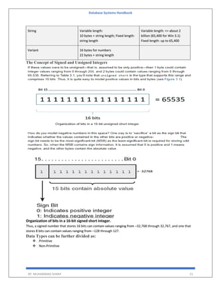
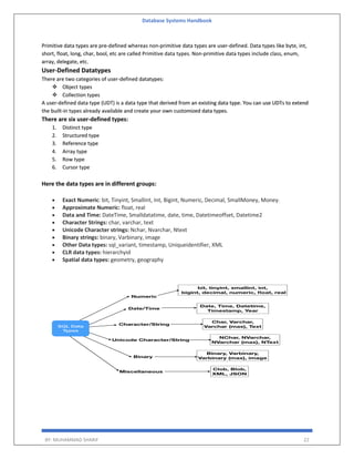
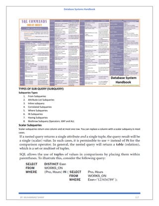
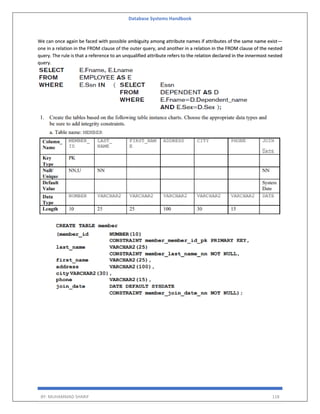
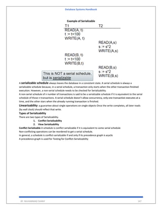
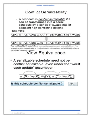
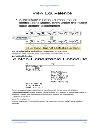
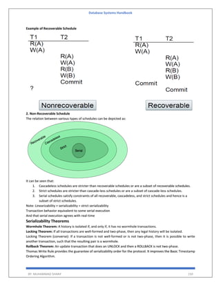
Download to read offline


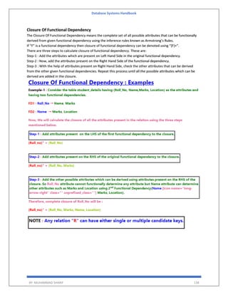

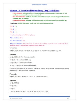
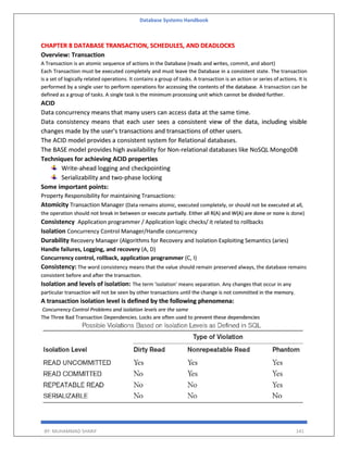
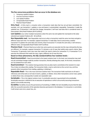
![Database Systems Handbook
BY: MUHAMMAD SHARIF 155
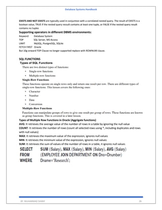
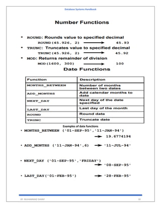
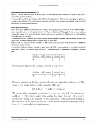
A[i,j] indicates the number of j the resource type allocated to I the process.
Request
Matrix of size n*m
Indicates the request of each process.
Request[i,j] tells the number of instances Pi process is the request of jth resource type.
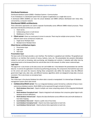
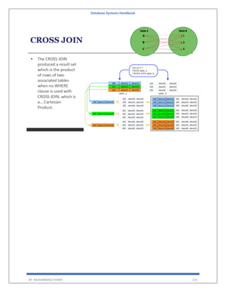
Deadlock Avoidance
Deadlock avoidance
Acquire locks in a pre-defined order
Acquire all locks at once before starting transactions
Aborting a transaction is not always a practical approach. Instead, deadlock avoidance mechanisms can be used to
detect any deadlock situation in advance.
The deadlock prevention technique avoids the conditions that lead to deadlocking. It requires that every
transaction lock all data items it needs in advance. If any of the items cannot be obtained, none of the items are
locked.
The transaction is then rescheduled for execution. The deadlock prevention technique is used in two-phase
locking.
To prevent any deadlock situation in the system, the DBMS aggressively inspects all the operations, where
transactions are about to execute. If it finds that a deadlock situation might occur, then that transaction is never
allowed to be executed.
Deadlock Prevention Algo
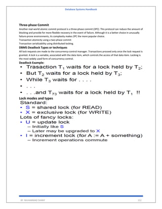
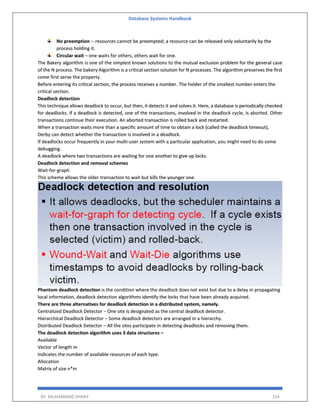
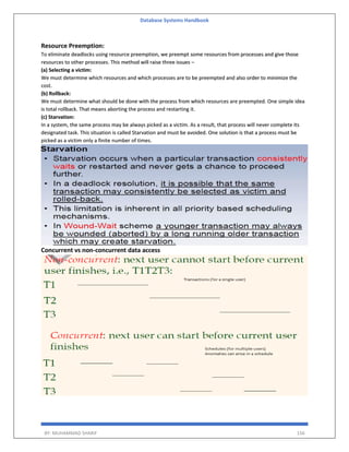
1. Wait-Die scheme
2. Wound wait scheme
Note! Deadlock prevention is more strict than Deadlock Avoidance.
The algorithms are as follows −
Wait-Die − If T1 is older than T2, T1 is allowed to wait. Otherwise, if T1 is younger than T2, T1 is aborted and later
restarted.
Wait-die: permit older waits for younger
Wound-Wait − If T1 is older than T2, T2 is aborted and later restarted. Otherwise, if T1 is younger than T2, T1 is
allowed to wait. Wound-wait: permit younger waits for older.
Note: In a bulky system, deadlock prevention techniques may work well.
Here, we want to develop an algorithm to avoid deadlock by making the right choice all the time
Dijkstra's Banker's Algorithm is an approach to trying to give processes as much as possible while guaranteeing
no deadlock.
safe state -- a state is safe if the system can allocate resources to each process in some order and still avoid a
deadlock.
Banker's Algorithm for Single Resource Type is a resource allocation and deadlock avoidance algorithm. This
name has been given since it is one of most problems in Banking Systems these days.
In this, as a new process P1 enters, it declares the maximum number of resources it needs.
The system looks at those and checks if allocating those resources to P1 will leave the system in a safe state or not.
If after allocation, it will be in a safe state, the resources are allocated to process P1.
Otherwise, P1 should wait till the other processes release some resources.
This is the basic idea of Banker’s Algorithm.
A state is safe if the system can allocate all resources requested by all processes ( up to their stated maximums )
without entering a deadlock state.](https://image.slidesharecdn.com/databasesystemshandbookbymuhammadsharif-220803040105-d53df9c4/85/Database-systems-Handbook-by-Muhammad-Sharif-pdf-155-320.jpg)

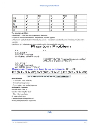


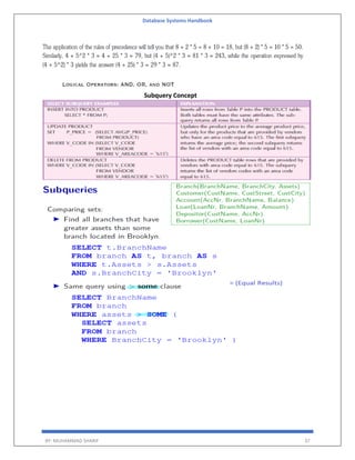
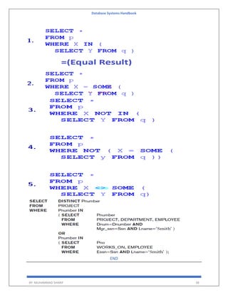
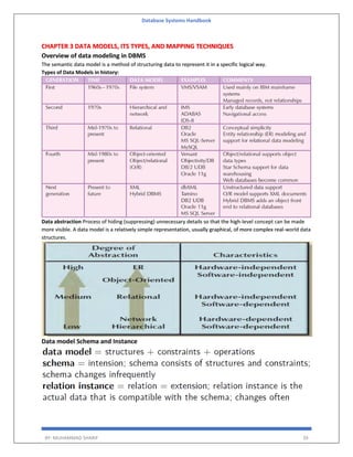
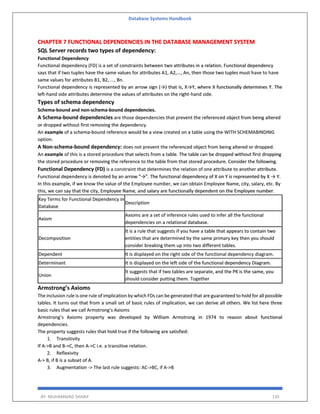
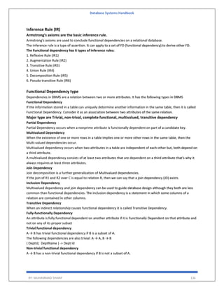
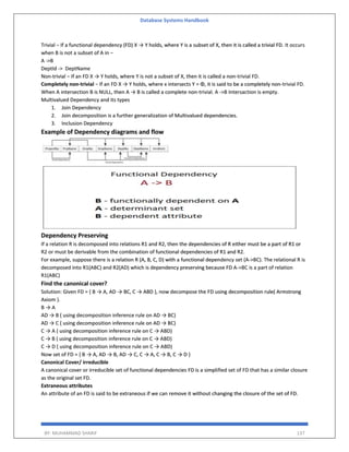
The 'Database Systems Handbook' by Muhammad Sharif provides an extensive overview of database concepts, including types of data, database management systems (DBMS), and the evolution of database architectures. It covers various topics such as structured and unstructured data, SQL functions, database design, and transaction management, while also discussing the challenges and solutions in transitioning from file systems to relational databases. Additionally, the handbook highlights distributed database systems, including client-server architectures and heterogeneous databases, emphasizing their operational efficiencies and complexities.