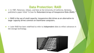
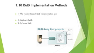
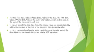
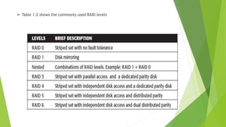
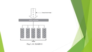
The document discusses data storage using RAID (Redundant Array of Independent Disks). It describes two main RAID implementation methods: hardware RAID which uses a specialized controller, and software RAID which is implemented at the operating system level. It also explains different RAID techniques like striping, mirroring, and parity to provide data redundancy. Several common RAID levels are defined based on these techniques, including RAID 0, 1, and nested RAID levels like RAID 1+0 which combine striping and mirroring for improved performance and redundancy.

1. Introduction to Information
Storage and
Management(17CS754)
© 2009 EMC Corporation. All rights reserved.
Module 1 : Chapter 3
By,
Madhura N K
Assistant professor
AITM, Bhatkal
Section 1 : Storage System

2. Data Protection: RAID
 ➢ In 1987, Patterson, Gibson, and Katz at the University of California, Berkeley,
published a paper titled “A Case for Redundant Arrays of Inexpensive Disks (RAID).”
 ➢ RAID is the use of small-capacity, inexpensive disk drives as an alternative to
large- capacity drives common on mainframe computers.
 ➢ Later RAID has been redefined to refer to independent disks to reflect advances in
the storage technology.

3. 1.10 RAID Implementation Methods
 ➢ The two methods of RAID implementation are:
 1. Hardware RAID.
 2. Software RAID

4. 1.10.1 Hardware RAID
 ➢ In hardware RAID implementations, a specialized hardware controller is
implemented either on the host or on the array.
 ➢ Controller card RAID is a host-based hardware RAID implementation in
which a specialized RAID controller is installed in the host, and disk drives
are connected to it.
 ➢ Manufacturers also integrate RAID controllers on motherboards.
 ➢ A host-based RAID controller is not an efficient solution in a data center
environment with a large number of hosts.
 ➢ The external RAID controller is an array-based hardware RAID.
 ➢ It acts as an interface between the host and disks.
 ➢ It presents storage volumes to the host, and the host manages these
volumes as physical drives

5.  ➢ The key functions of the RAID controllers are as follows:
 ✓ Management and control of disk aggregations
 ✓ Translation of I/O requests between logical disks and physical disks
 ✓ Data regeneration in the event of disk failures.
Components of RAID array

6. 1.10.2 Software RAID
 ➢ Software RAID uses host-based software to provide RAID functions.
 ➢ It is implemented at the operating-system level and does not use a dedicated
hardware controller to manage the RAID array.
 ➢ Advantages when compared to Hardware RAID:
 ✓ cost
 ✓ simplicity benefits
 ➢ Limitations:
 ✓ Performance: Software RAID affects overall system performance. This is due to
additional CPU cycles required to perform RAID calculations.
 ✓ Supported features: does not support all RAID levels.
 ✓ Operating system compatibility: Software RAID is tied to the host operating
system; hence, upgrades to software RAID or to the operating system should be
validated for compatibility.

7. RAID Techniques
 ➢ There are three RAID techniques
 1. Striping
 2. Mirroring
 3. Parity

8. Striping
 Striping is a technique to spread data across multiple drives (more than one) to use the
drives in parallel.
 􀂾 All the read-write heads work simultaneously, allowing more data to be processed in a
shorter time and increasing performance, compared to reading and writing from a single
disk.
 􀂾 Within each disk in a RAID set, a predefined number of contiguously addressable disk
blocks are defined as a strip.
 􀂾 The set of aligned strips that spans across all the disks within the RAID set is called a
stripe.

9. Fig 1.11 shows physical and logical representations of a striped RAID set.

10.  Strip size (also called stripe depth) describes the number of blocks in a
strip and is the maximum amount of data that can be written to or read
from a single disk in the set.
 􀂾 All strips in a stripe have the same number of blocks.
 􀂾 Having a smaller strip size means that data is broken into smaller pieces
while spread across the disks.
 􀂾 Stripe size is a multiple of strip size by the number of data disks in the
RAID set.
 􀂾 Eg: In a 5 disk striped RAID set with a strip size of 64 KB, the stripe size is
320KB (64KB x 5).
 􀂾 Stripe width refers to the number of data strips in a stripe.
 􀂾 Striped RAID does not provide any data protection unless parity or
mirroring is used.

12. Fig 1.12: Mirrored disks in an array

13.  Advantages:
 ✓ complete data redundancy,
 ✓ mirroring enables fast recovery from disk failure.
 ✓ data protection
 ➢ Mirroring is not a substitute for data backup. Mirroring constantly
captures changes in the data, whereas a backup captures point-in-time
images of the data.
 ➢ Disadvantages:
 ✓ Mirroring involves duplication of data — the amount of storage capacity
needed is twice the amount of data being stored.
 ✓ Expensive

14. 1.11.3 Parity
 Parity is a method to protect striped data from disk drive failure without the cost of
 mirroring.
 ➢ An additional disk drive is added to hold parity, a mathematical construct that
allows recreation of the missing data.
 ➢ Parity is a redundancy technique that ensures protection of data without
maintaining a full set of duplicate data.
 ➢ Calculation of parity is a function of the RAID controller.
 ➢ Parity information can be stored on separate, dedicated disk drives or distributed
across all the drives in a RAID set.

15. Fig 1.13: Parity RAID

16.  The first four disks, labeled “Data Disks,” contain the data. The fifth disk,
labeled “Parity Disk,” stores the parity information, which, in this case, is
the sum of the elements in each row.
 ➢ Now, if one of the data disks fails, the missing value can be calculated by
subtracting the sum of the rest of the elements from the parity value.
 ➢ Here, computation of parity is represented as an arithmetic sum of the
data. However, parity calculation is a bitwise XOR operation.

17.  XOR Operation:
 ➢ A bit-by-bit Exclusive -OR (XOR) operation takes two bit patterns of equal
length and performs the logical XOR operation on each pair of corresponding
bits.
 ➢ The result in each position is 1 if the two bits are different, and 0 if they
are the same.
 ➢ The truth table of the XOR operation is shown below (A and B denote
inputs and C, the output the XOR operation).

19.  If any of the data from A, B, or C is lost, it can be reproduced by performing an XOR
operation on the remaining available data.
 ➢ Eg: if a disk containing all the data from A fails, the data can be regenerated by
performing an XOR between B and C.
 ➢ Advantages:
 ✓ Compared to mirroring, parity implementation considerably reduces the cost
associated with data protection.
 ➢ Disadvantages:
 ✓ Parity information is generated from data on the data disk. Therefore, parity is
recalculated every time there is a change in data.
 ✓ This recalculation is time-consuming and affects the performance of the RAID array.
 ➢ For parity RAID, the stripe size calculation does not include the parity strip.
 ➢ Eg: in a five (4 + 1) disk parity RAID set with a strip size of 64 KB, the stripe size will
be 256KB (64 KB x 4).

20. 1.12 RAID Levels
➢ RAID Level selection is determined by below factors:
 ✓ Application performance
 ✓ data availability requirements
 ✓ cost
➢ RAID Levels are defined on the basis of:
 ✓ Striping
 ✓ Mirroring
 ✓ Parity techniques
 ➢ Some RAID levels use a single technique whereas others use a
combination of techniques.

21. ➢ Table 1.2 shows the commonly used RAID levels

22. 1.12.1 RAID 0
 RAID 0 configuration uses data striping techniques, where data is striped across all
the disks
 within a RAID set. Therefore it utilizes the full storage capacity of a RAID set.
 ➢ To read data, all the strips are put back together by the controller.
Fig 1.14 shows RAID 0 in an array in which data is striped across five disks.
When the number of drives in the RAID set increases, performance improves because
more data can be read or written simultaneously.
➢ RAID 0 is a good option for applications that need high I/O throughput.
➢ However, if these applications require high availability during drive failures, RAID
0 does not provide data protection and availability.

24. 1.12.2 RAID 1
 RAID 1 is based on the mirroring technique.
 ➢ In this RAID configuration, data is mirrored to provide fault tolerance (see
Fig 1.15).
 A RAID 1 set consists of two disk drives and every write is written to both
disks.
 ➢ The mirroring is transparent to the host.
 ➢ During disk failure, the impact on data recovery in RAID 1 is the least
among all RAID implementations. This is because the RAID controller uses
the mirror drive for data recovery.
 ➢ RAID 1 is suitable for applications that require high availability and cost is
no constraint.

25. Fig 1.15: RAID 1

26. 1.12.3 Nested RAID
 Most data centers require data redundancy and performance from their RAID
arrays.
 ➢ RAID 1+0 and RAID 0+1 combine the performance benefits of RAID 0 with
the redundancy benefits of RAID 1.
 ➢ They use striping and mirroring techniques and combine their benefits.
 ➢ These types of RAID require an even number of disks, the minimum being
four (see Fig1.16).

28. RAID 1+0:
 ➢ RAID 1+0 is also known as RAID 10 (Ten) or RAID 1/0.
 ➢ RAID 1+0 performs well for workloads with small, random, write-intensive I/Os.
 ➢ Some applications that benefit from RAID 1+0 include the following:
 ✓ High transaction rate Online Transaction Processing (OLTP)
 ✓ Large messaging installations
 ✓ Database applications with write intensive random access workloads
 ➢ RAID 1+0 is also called striped mirror.
 ➢ The basic element of RAID 1+0 is a mirrored pair, which means that data is first
mirrored and then both copies of the data are striped across multiple disk drive pairs in
a RAID set.
 ➢ When replacing a failed drive, only the mirror is rebuilt. The disk array controller
uses the surviving drive in the mirrored pair for data recovery and continuous operation.

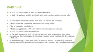
29.  Working of RAID 1+0:
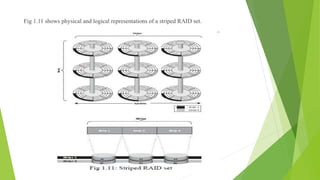
 ➢ Eg: consider an example of six disks forming a RAID 1+0 (RAID 1 first and
then RAID 0)set.
 ➢ These six disks are paired into three sets of two disks, where each set
acts as a RAID 1 set(mirrored pair of disks). Data is then striped across all
the three mirrored sets to form RAID 0.
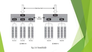
 Following are the steps performed in RAID 1+0 (see Fig 1.16 [a]):
 ✓ Drives 1+2 = RAID 1 (Mirror Set A)
 ✓ Drives 3+4 = RAID 1 (Mirror Set B)
 ✓ Drives 5+6 = RAID 1 (Mirror Set C)
 ➢ Now, RAID 0 striping is performed across sets A through C.

30.  Now, RAID 0 striping is performed across sets A through C.
 ➢ In this configuration, if drive 5 fails, then the mirror set C alone is affected. It
still has drive 6 and continues to function and the entire RAID 1+0 array also keeps
functioning.
 ➢ Now, suppose drive 3 fails while drive 5 was being replaced. In this case the
array still continues to function because drive 3 is in a different mirror set.
 ➢ So, in this configuration, up to three drives can fail without affecting the array,
as long as they are all in different mirror sets.
 ➢ RAID 0+1 is also called a mirrored stripe.
 ➢ The basic element of RAID 0+1 is a stripe. This means that the process of
striping data across disk drives is performed initially, and then the entire stripe is
mirrored.
 ➢ In this configuration if one drive fails, then the entire stripe is faulted.

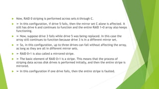
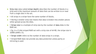
31.  Working of RAID 0+1:
 ➢ Eg: Consider the same example of six disks forming a RAID 0+1 (that is,
RAID 0 first and then RAID 1).
 ➢ Here, six disks are paired into two sets of three disks each.
 ➢ Each of these sets, in turn, act as a RAID 0 set that contains three disks
and then these two sets are mirrored to form RAID 1.
 ➢ Following are the steps performed in RAID 0+1 (see Fig 1.16 [b]):
 ✓ Drives 1 + 2 + 3 = RAID 0 (Stripe Set A)
 ✓ Drives 4 + 5 + 6 = RAID 0 (Stripe Set B)

32.  These two stripe sets are mirrored.
 ➢ If one of the drives, say drive 3, fails, the entire stripe set A fails.
 ➢ A rebuild operation copies the entire stripe, copying the data from each
disk in the healthy stripe to an equivalent disk in the failed stripe.
 ➢ This causes increased and unnecessary I/O load on the surviving disks and
makes the RAID set more vulnerable to a second disk failure.

33. 1.12.4 RAID 3
 RAID 3 stripes data for high performance and uses parity for improved fault
tolerance.
 ➢ Parity information is stored on a dedicated drive so that data can be
reconstructed if a drive fails. For example, of five disks, four are used for
data and one is used for parity.
 ➢ RAID 3 always reads and writes complete stripes of data across all disks,
as the drives operate in parallel. There are no partial writes that update one
out of many strips in a stripe.
 ➢ RAID 3 provides good bandwidth for the transfer of large volumes of data.
RAID 3 is used in applications that involve large sequential data access, such
as video streaming.

34. ➢ Fig 1.17 shows the RAID 3 implementation
Fig 1.17: RAID 3

35. 1.12.5 RAID 4
 RAID 4 stripes data for high performance and uses parity for improved fault
tolerance. Data is striped across all disks except the parity disk in the array.
 ➢ Parity information is stored on a dedicated disk so that the data can be
rebuilt if a drive fails.
 Striping is done at the block level.
 Unlike RAID 3, data disks in RAID 4 can be accessed independently so that
specific data elements can be read or written on single disk without read or
write of an entire stripe. RAID
 4 provides good read throughput and reasonable write throughput.

36. 1.12.6 RAID 5
 RAID 5 is a versatile RAID implementation.
 ➢ It is similar to RAID 4 because it uses striping. The drives (strips) are also
independently accessible.
 ➢ The difference between RAID 4 and RAID 5 is the parity location. In RAID 4, parity
is written to a dedicated drive, creating a write bottleneck for the parity disk
 ➢ In RAID 5, parity is distributed across all disks. The distribution of parity in RAID 5
overcomes the Write bottleneck. Below Figure illustrates the RAID 5 implementation.
 ➢ Fig 1.18 illustrates the RAID 5 implementation.
 ➢ RAID 5 is good for random, read-intensive I/O applications and preferred for
messaging, data mining, medium-performance media serving, and relational
database management system (RDBMS) implementations, in which database
administrators (DBAs) optimize data access.

37. Fig 1.18: RAID 5

38. 1.12.7 RAID 6
 RAID 6 includes a second parity element to enable survival in the event of
the failure of two disks in a RAID group. Therefore, a RAID 6 implementation
requires at least four disks.
 ➢ RAID 6 distributes the parity across all the disks. The write penalty in
RAID 6 is more than that in RAID 5; therefore, RAID 5 writes perform better
than RAID 6. The rebuild operation in RAID 6 may take longer than that in
RAID 5 due to the presence of two parity sets.

39. ➢ Fig 1.19 illustrates the RAID 6 implementation
Fig 1.19: RAID 6

40. 1.13 RAID Impact on Disk Performance
 When choosing a RAID type, it is imperative to consider its impact on disk
performance and application IOPS.
 ➢ In both mirrored (RAID 1) and parity RAID (RAID 5) configurations, every
write operation translates into more I/O overhead for the disks which is
referred to as write penalty.
 ➢ In a RAID 1 implementation, every write operation must be performed on
two disks configured as a mirrored pair. The write penalty is 2.
 ➢ In a RAID 5 implementation, a write operation may manifest as four I/O
operations. When performing small I/Os to a disk configured with RAID 5,
the controller has to read, calculate,and write a parity segment for every
data write operation.

41. Fig 1.20 illustrates a single write operation
on RAID 5 that contains a group of five disks.

42.  Four of these disks are used for data and one is used for parity.
 ➢ The parity (Ep) at the controller is calculated as follows:
Ep = E1 + E2 + E3 + E4 (XOR operations)
 ➢ Whenever the controller performs a write I/O, parity must be computed by reading the old parity
(Ep old) and the old data (E4 old) from the disk, which means two read I/Os.
➢ The new parity (Ep new) is computed as follows:
Ep new = Ep old – E4 old + E4 new (XOR operations)
➢ After computing the new parity, the controller completes the write I/O by doing two write
I/Os for the new data and the new parity onto the disks..
 ➢ Therefore,In RAID 5 the controller performs two disk reads and two disk writes for every write
operation, and the write penalty is 4.
 ➢ In RAID 6, which maintains dual parity, a disk write requires three read operations: two
parity and one data.
 ➢ After calculating both new parities, the controller performs three write operations: two
parity and an I/O.
 ➢ Therefore, in a RAID 6 implementation, the controller performs six I/O operations for
each write I/O, and the write penalty is 6.