UNIVERSITY COLLEGE OFENGINEERING PATTUKKOTTAI
(A Constituent College Of Anna University::Chennai-25)
Rajamadam – 614701
Department of Computer Science and Engineering
Record Note Book
CS3481: Database Management Systems Laboratory
2.
UNIVERSITY COLLEGE OFENGINEERING PATTUKKOTTAI
(A Constituent College Of Anna University::Chennai-25)
Rajamadam – 614701
Department of Computer Science and Engineering
Record Note Book
Name :
Register Number :
Subject Code / Subject Name
Semester
Branch
Academic Year
: CS3481 / Database Management Systems Lab
: IV
: CSE- II Year
: 2024- 2025
3.
UNIVERSITY COLLEGE OFENGINEERING PATTUKKOTTAI
(A Constituent College Of Anna University::Chennai-25)
Rajamadam – 614701
Department of Computer Science and Engineering
BONAFIDE CERTIFICATE
Certified to be the bonafide record of work done by Mr/Ms
…………………………………………… with Register Number
Computer Science and Engineering branch during the Academic Year
Staff Incharge Head of the Department
Submitted for the University Practical Examination held on
………………………….. at University College Of Engineering, Pattukkottai,
Rajamadam.
Internal Examiner External Examiner
...............................................for CS 3481 : Database Management Systems
2024 - 2025
Laboratory II -Year in IV- Semester of B.E Degree Courses in
Ex.No.:01
SQL DDL andDML Commands, SQL Constraints
Date:
Aim:
To create a database table, add constraints (primary key, unique, check, Not null),
insert rows, update and delete rows using SQL DDL and DML commands.
Description:
Structured query language (SQL) is a programming language for storing and
processing information in a relational database. SQL statements are used to store, update,
remove, search, and retrieve information from the database.
These SQL commands are mainly categorized into five categories as:
1. DDL – Data Definition Language
2. DQL –
3. DML –
4. DCL –
5. TCL –
DDL – Data Definition Language
Data Definition Language consists of the SQL commands that can be used to define
the database schema. It simply deals with descriptions of the database schema and is used to
create and modify the structure of database objects in the database. DDL is a set of SQL
commands used to create, modify, and delete database structures but not data. These
commands are normally not used by a general user, who should be accessing the database
via an application.
DDL commands:
1. CREATE: This command is used to create the database or its objects (like table, index,
function, views, store procedure, and triggers).
name(column_1 datatype, column_2 datatype,
column_3 datatype, ....);
2. DROP: This command is used to delete objects from the database.
Syntax: DROP TABLE table_name;
3. ALTER: This is used to alter the structure of the database.
Syntax: To add new column in the table
ALTER TABLE table_name ADD column_name datatype;
To change the datatype of a column in the table:
ALTER TABLE table_name MODIFY COLUMN column_name datatype;
8.
To drop columnsin a table:
ALTER TABLE table_name DROP COLUMN column_name;
To rename a column in a table:
ALTER TABLE table_name RENAME COLUMN old_name to new_name;
4. TRUNCATE: This is used to remove all records from a table, including all spaces
allocated for the records are removed.
Syntax: TRUNCATE TABLE table_name;
5. COMMENT: This is used to add comments to the data dictionary.
6. RENAME: This is used to rename an object existing in the database.
Syntax: ALTER TABLE table_name RENAME TO new_table_name;
DML - Data Manipulation Language
The SQL commands that deals with the manipulation of data present in the database belong
to DML or Data Manipulation Language and this includes most of the SQL statements. It is
the component of the SQL statement that controls access to data and to the database.
Basically, DCL statements are grouped with DML statements.
List of DML commands:
1. INSERT: It is used to insert data into a table.
Syntax: INSERT INTO TABLE_NAME (col1, col2, col3,.... col N) VALUES (value1,
value2, value3, .... valueN);
Or
INSERT INTO TABLE_NAME
VALUES (value1, value2, value3, .... valueN);
2. UPDATE: It is used to update existing data within a table.
Syntax: UPDATE table_name SET [column_name1= value1,...column_nameN =
valueN] [WHERE CONDITION]
3. DELETE: It is used to delete records from a database table.
Syntax: DELETE FROM table_name [WHERE condition];
SQL Constraints
SQL constraints are used to specify rules for the data in a table.Constraints are used to
limit the type of data that can go into a table. This ensures the accuracy and reliability of the
data in the table. If there is any violation between the constraint and the data action, the
action is aborted.
Constraints can be column level or table level. Column level constraints apply to a
column, and table level constraints apply to the whole table.
9.
The following constraintsare commonly used in SQL:
1. NOT NULL - Ensures that a column cannot have a NULL value.
2. UNIQUE - Ensures that all values in a column are different.
3. PRIMARY KEY - A combination of NOT NULL and UNIQUE. Uniquely identifies
each row in a table.
4. FOREIGN KEY - Prevents actions that would destroy links between tables.
5. CHECK - Ensures that the values in a column satisfies a specific condition.
6. DEFAULT - Sets a default value for a column if no value is specified.
7. CREATE INDEX - Used to create and retrieve data from the database very quickly.
SQL Create Constraints
Constraints can be specified when the table is created with the CREATE TABLE
statement, or after the table is created with the ALTER TABLE statement.
Syntax: CREATE TABLE table_name (column1 datatype constraint, column2 datatype
constraint, column3 datatype constraint, .... );
Queries on DDL and DML commands:
Table creation with constraints:
SQL> create schema dbmslab;
SQL> use dbmslab;
SQL> create table emp_details(emp_no int(10) primary key, emp_name varchar(20) not null,
age int(3) check(age>=20), address varchar(30), doj varchar(10), mobile_no int(12) unique,
dept_no int(5) not null, salary int(10));
Output: 0 row(s) affected.
SQL> alter table emp_details modify column mobile_no varchar(10);
Output: 0 row(s) affected Records:0 Duplicates:0 Warnings:0
SQL> insert into emp_details values(101,'SSS',25, 'Chennai', '01/01/2000', '9823578900', 563,
10000);
Output: 1 row(s) affected.
SQL> insert into emp_details(emp_no, emp_name, age, address, doj, mobile_no, dept_no,
salary) values (102, 'RRR', 20, 'Salem', '24/06/2017', '9175368421', 563, 7500), (103, 'FFF', 30,
'Salem', '24/07/2000', '7875368421', 541, 20000), (104, 'XXX', 35, 'Erode', '06/07/2001',
'7894563421', 563, 25000);
Output: 3 row(s) affected Records:3 Duplicates:0 Warnings:0
SQL> select * from emp_details;
10.
Output: 4 row(s)returned
emp_
no
emp_name age address doj mobile_no dept_
no
salary
101 SSS 25 Chennai 01/01/2000 9823578900 563 10000
102 RRR 20 Salem 24/06/2017 9175368421 563 7500
103 FFF 30 Salem 24/07/2000 7875368421 541 20000
104 XXX 35 Erode 06/07/2001 7894563421 563 25000
SQL> update emp_details set salary=26000 where emp_no=104;
Output: 1 row(s) affected Rows matched:1 Changed:1 Warnings:0
SQL> select * from emp_details;
Output: 4 row(s) returned
emp_
no
emp_name age address doj mobile_no dept_
no
salary
101 SSS 25 Chennai 01/01/2000 9823578900 563 10000
102 RRR 20 Salem 24/06/2017 9175368421 563 7500
103 FFF 30 Salem 24/07/2000 7875368421 541 20000
104 XXX 35 Erode 06/07/2001 7894563421 563 26000
SQL> delete from emp_details where emp_no=102;
Output: 1 row(s) affected
SQL> select * from emp_details;
Output: 3 row(s) affected
emp_
no
emp_name age address doj mobile_no dept_
no
salary
101 SSS 25 Chennai 01/01/2000 9823578900 563 10000
103 FFF 30 Salem 24/07/2000 7875368421 541 20000
11.
104 XXX 35Erode 06/07/2001 7894563421 563 26000
SQL> alter table emp_details drop column salary;
Output: 0 row(s) affected Records:0 Duplicates:0 Warnings:0
SQL> select * from emp_details;
Output: 3 row(s) returned
emp_no emp_name age address doj mobile_no dept_no
101 SSS 25 Chennai 01/01/2000 9823578900 563
103 FFF 30 Salem 24/07/2000 7875368421 541
104 XXX 35 Erode 06/07/2001 7894563421 563
SQL> truncate table emp_details;
Output: 0 row(s) affected
SQL> select * from emp_details;
Output: 0 row(s) returned
emp_no emp_name age address doj mobile_no dept_no
SQL> drop table emp_details;
Output: 0 row(s) affected
SQL> select * from emp_details;
Output: Error Code: 1146. Table 'dbmslab.emp_details' doesn't exist
Result:
Thus the database table with constraints has been created and various DDL and DML
commands have been executed successfully.
12.
Ex.No.:02
Referential Integrity
Date:
Aim:
To createa set of tables, add foreign key constraints and incorporate referential
integrity.
Description:
Referential integrity refers to the relationship between tables. Because each table in a
database must have a primary key, this primary key can appear in other tables because of its
relationship to data within those tables. When a primary key from one table appears in
another table, it is called a foreign key.
The table containing the foreign key is called the child table(Referencing Table), and
the table containing the Primary key/candidate key is called the master or parent
table(Referenced Table).
The essential syntax for a defining a foreign key constraint in a CREATE TABLE or
ALTER TABLE statement includes the following:
Syntax: [CONSTRAINT [symbol]] FOREIGN KEY [index_name] (col_name, ...)
REFERENCES tbl_name (col_name,...) [ON DELETE reference_option] [ON UPDATE
reference_option]
reference_option:
RESTRICT | CASCADE | SET NULL | NO ACTION | SET DEFAULT
Referential Actions
When an UPDATE or DELETE operation affects a key value in the parent table that
has matching rows in the child table, the result depends on the referential action specified by
ON UPDATE and ON DELETE subclauses of the FOREIGN KEY clause.
Referential actions include:
CASCADE: Delete or update the row from the parent table and automatically delete or
update the matching rows in the child table. Both ON DELETE CASCADE and ON UPDATE
CASCADE are supported. Between two tables, do not define several ON UPDATE
CASCADE clauses that act on the same column in the parent table or in the child table.
If an ON UPDATE CASCADE or ON DELETE CASCADE subclause is only defined
for one FOREIGN KEY clause, cascading operations fail with an error.
Note:Cascaded foreign key actions do not activate triggers.
13.
SET NULL: Deleteor update the row from the parent table and set the foreign key column or
columns in the child table to NULL. Both ON DELETE SET NULL and ON UPDATE SET
NULL clauses are supported.
RESTRICT: Rejects the delete or update operation for the parent table. Specifying RESTRICT
(or NO ACTION) is the same as omitting the ON DELETE or ON UPDATE clause.
NO ACTION: A keyword from standard SQL. In MySQL, equivalent to RESTRICT. Some
database systems have deferred checks, and NO ACTION is a deferred check. In MySQL,
foreign key constraints are checked immediately, so NO ACTION is the same as RESTRICT.
SET DEFAULT: This action is recognized by the MySQL parser, but both InnoDB and NDB
reject table definitions containing ON DELETE SET DEFAULT or ON UPDATE SET
DEFAULT clauses.
For storage engines that support foreign keys, MySQL rejects any INSERT or
UPDATE operation that attempts to create a foreign key value in a child table if there is no
matching candidate key value in the parent table.
For an ON DELETE or ON UPDATE that is not specified, the default action is always
NO ACTION.
Adding Foreign Key Constraints
A foreign key constraint can be added to an existing table using ALTER TABLE
syntax:
Syntax: ALTER TABLE tbl_name ADD [CONSTRAINT [symbol]] FOREIGN KEY
[index_name] (col_name, ...) REFERENCES tbl_name (col_name,...) [ON DELETE
reference_option] [ON UPDATE reference_option];
Dropping Foreign Key Constraints
A foreign key constraint can be dropped using ALTER TABLE syntax:
Syntax: ALTER TABLE tbl_name DROP FOREIGN KEY fk_symbol;
Queries:
SQL> create table product (category int not null, id int not null, price decimal, primary
key(category, id));
Output: 0 row(s) affected
SQL> create table customer (id int not null, primary key(id));
Output: 0 row(s) affected
SQL> create table product_order (no int not null auto_increment, product_category int not
null, product_id int not null, customer_id int not null, primary key(no), index
(product_category, product_id), index (customer_id), foreign key (product_category,
14.
product_id) references product(category,id) ON UPDATE CASCADE ON DELETE
RESTRICT, foreign key (customer_id) references customer(id));
Output: 0 row(s) affected
SQL> insert into product (category, id, price) values (542,1001,25.89), (542,1002,40),
(543,1003,80);
Output: 3 row(s) affected Records:3 Duplicates:0 Warnings:0
SQL> select * from product;
Output: 3 row(s) returned
category id price
542 1001 26
542 1002 40
543 1003 80
SQL> insert into customer(id) values(121),(123),(124);
Output: 3 row(s) affected Records:3 Duplicates:0 Warnings:0
SQL> select * from customer;
Output: 3 row(s) returned
id
121
123
124
SQL> insert into product_order values(1, 542, 1001,121);
Output: 1 row(s) affected
SQL> insert into product_order values(2, 555,1001,121);
Output: Error Code: 1452. Cannot add or update a child row: a foreign key constraint
fails (`dbmslab`.`product_order`, CONSTRAINT `product_order_ibfk_1` FOREIGN KEY
(`product_category`, `product_id`) REFERENCES `product` (`category`, `id`) ON DELETE
RESTRICT ON UPDATE CASCADE)
SQL> insert into product_order values(2, 542,1001,121);
15.
Output: 1 row(s)affected
SQL> insert into product_order values(2, 543,1002,123);
Output: Error Code: 1062. Duplicate entry '2' for key 'product_order.PRIMARY'
SQL> select * from product_order;
Output: 2 row(s) returned
no product_category product_id customer_id
1 542 1001 121
2 542 1001 121
SQL> delete from customer where id=121;
Output: Error Code: 1451. Cannot delete or update a parent row: a foreign key
constraint fails (`dbmslab`.`product_order`, CONSTRAINT `product_order_ibfk_2`
FOREIGN KEY (`customer_id`) REFERENCES `customer` (`id`))
SQL> delete from product_order where customer_id=121;
Output: 2 row(s) affected
SQL> select * from product_order;
Output: 0 row(s) returned
no product_category product_id customer_id
SQL> delete from customer where id=121;
Output: 1 row(s) affected
SQL> select * from customer;
Output: 2 row(s) returned
id
123
124
Result:
Thus a set of tables have been created, added foreign keys and incorporated
referential integrity successfully.
16.
Ex.No.:03
Basic Operations andAggregate Functions
Date:
Aim:
To query the database tables using ‘where’ clause conditions and to implement basic
SQL operations and various aggregate functions.
Description:
The SQL WHERE Clause: The WHERE clause is used to filter records. It is used to extract
only those records that fulfill a specified condition. The WHERE clause is not only used in
SELECT statements, it is also used in UPDATE, DELETE, etc.
Syntax: SELECT column1, column2, … FROM table_name WHERE condition;
Operators used in The WHERE Clause are Equal(=), Greater than (>), Less than (<),
Greater than or equal (>=), Less than or equal (<=), Not equal (<> or !=), BETWEEN
(Between a certain range), LIKE (Search for a pattern), IN (To specify multiple possible
values for a column).
Basic operations:
Rename or Aliases
SQL aliases or rename are used to give a table, or a column in a table, a temporary
name. Aliases are often used to make column names more readable. An alias only exists for
the duration of that query. An alias is created with the AS keyword.
Syntax for renaming column
SELECT column_name AS alias_name FROM table_name;
Alias Table Syntax
SELECT column_name(s) FROM table_name AS alias_name;
LIKE operator
The LIKE operator is used in a WHERE clause to search for a specified pattern in a
column.
There are two wildcards often used in conjunction with the LIKE operator:
● The percent sign (%) represents zero, one, or multiple characters
● The underscore sign (_) represents one, single character
Syntax
SELECT column1, column2, … FROM table_name WHERE column LIKE pattern;
Some examples showing different LIKE operators with '%' and '_' wildcards:
17.
LIKE Operator Description
WHERECustomerName LIKE 'a%' Finds any values that start with "a"
WHERE CustomerName LIKE '%a' Finds any values that end with "a"
WHERE CustomerName LIKE '%or%' Finds any values that have "or" in any position
WHERE CustomerName LIKE '_r%' Finds any values that have "r" in the second
position
WHERE CustomerName LIKE 'a_%' Finds any values that start with "a" and are at
least 2 characters in length
WHERE CustomerName LIKE 'a_ _%' Finds any values that start with "a" and are at
least 3 characters in length
WHERE ContactName LIKE 'a%o' Finds any values that start with "a" and ends
with "o"
ORDER BY operator
The ORDER BY keyword is used to sort the result-set in ascending or descending
order. The ORDER BY keyword sorts the records in ascending order by default. To sort the
records in descending order, use the DESC keyword.
Syntax: SELECT column1, column2, … FROM table_name ORDER BY column1,
column2, … ASC|DESC;
BETWEEN/NOT BETWEEN operator
The BETWEEN operator selects values within a given range. The values can be
numbers, text, or dates. The BETWEEN operator is inclusive: begin and end values are
included. NOT BETWEEN operator does not include begin and end values.
Syntax: SELECT column_name(s) FROM table_name WHERE column_name
BETWEEN/NOT BETWEEN value1 AND value2;
Set operators
Set operators combine the results of two component queries into a single result.
Queries containing set operators are called compound queries.
Operator Returns
UNION All distinct rows selected by either query
18.
UNION ALL Allrows selected by either query, including all duplicates
INTERSECT All distinct rows selected by both queries
MINUS/EXCEPT All distinct rows selected by the first query but not the second
AND, OR, NOT operators
The WHERE clause can be combined with AND, OR, and NOT operators.
The AND and OR operators are used to filter records based on more than one
condition:
● The AND operator displays a record if all the conditions separated by AND are TRUE.
● The OR operator displays a record if any of the conditions separated by OR is TRUE.
● The NOT operator displays a record if the condition(s) is NOT TRUE.
AND Syntax : SELECT column1, column2, … FROM table_name WHERE condition1
AND condition2 AND condition3 ...;
OR Syntax : SELECT column1, column2, … FROM table_name WHERE condition1
OR condition2 OR condition3 ...;
NOT Syntax : SELECT column1, column2, … FROM table_name WHERE NOT
condition;
Aggregate Function: An aggregate function is a function where the values of multiple rows
are grouped together as input on certain criteria to form a single value of more significant
meaning. Aggregate functions are often used with the GROUP BY and HAVING clauses of
the SELECT statement.
All the aggregate functions are used in the Select statement.
Syntax: SELECT <FUNCTION NAME> (<PARAMETER>) FROM <TABLE NAME>
Common aggregate functions are as follows:
1. COUNT(): The count function returns the number of rows in the result. It does not
count the null values.
Types
COUNT(*): Counts all the number of rows of the table including null.
COUNT( COLUMN_NAME): count number of non-null values in column.
COUNT( DISTINCT COLUMN_NAME): count number of distinct values in a column.
Syntax : COUNT() or COUNT([ALL|DISTINCT] expression)
19.
2. AVG(): TheAVG function is used to calculate the average value of the numeric type.
AVG function returns the average of all non-Null values.
Syntax: AVG() or AVG( [ALL|DISTINCT] expression )
3. MIN(): MIN function is used to find the minimum value of a certain column. This
function determines the smallest value of all selected values of a column.
Syntax: MIN() or MIN( [ALL|DISTINCT] expression )
4. MAX(): MAX function is used to find the maximum value of a certain column. This
function determines the largest value of all selected values of a column.
Syntax: MAX() or MAX( [ALL|DISTINCT] expression )
5. SUM(): Sum function is used to calculate the sum of all selected columns. It works on
numeric fields only.
Syntax: SUM() or SUM( [ALL|DISTINCT] expression )
Aggregation with GROUP BY
The GROUP BY statement groups rows that have the same values.
Syntax : SELECT column_name(s) FROM table_name WHERE condition
GROUP BY column_name(s);
HAVING clause
The HAVING clause was added to SQL because the WHERE keyword cannot be used
with aggregate functions.
Syntax : SELECT column_name(s) FROM table_name WHERE condition GROUP BY
column_name(s) HAVING condition;
Queries:
Sample table: PRODUCT_MAST
PRODUCT COMPANY QTY RATE COST
Item1 Com1 2 10 20
Item2 Com2 3 25 75
Item3 Com1 2 30 60
Item4 Com3 5 10 50
Item5 Com2 2 20 40
Item6 Com1 3 25 75
20.
Item7 Com1 530 150
Item8 Com1 3 10 30
Item9 Com2 2 25 50
Item10 Com3 4 30 120
SQL> select company, cost as price from product_mast order by cost;
Output : 10 row(s) returned
company price
Com1 20
Com1 30
Com2 40
Com3 50
Com2 50
Com1 60
Com2 75
Com1 75
Com3 120
Com1 150
SQL> select product from product_mast as t where company='Com1';
Output : 5 row(s) returned
PRODUCT
Item1
Item3
Item6
Item7
Item8
21.
SQL> select company,cost from product_mast where cost between 75 and 150;
Output : 4 row(s) returned
company price
Com2 75
Com1 75
Com3 120
Com1 150
SQL> select * from product_mast where rate not between 20 and 25;
Output: 6 row(s) returned
product company qty rate cost
Item1 Com1 2 10 20
Item3 Com1 2 30 60
Item4 Com3 5 10 50
Item7 Com1 5 30 150
Item8 Com1 3 10 30
Item10 Com3 4 30 120
SQL> select * from product_mast where qty>2 union select * from product_mast where
cost>50;
Output: 7 row(s) returned.
product company qty rate cost
Item2 Com2 3 25 75
Item4 Com3 5 10 50
Item6 Com1 3 25 75
Item7 Com1 5 30 150
Item8 Com1 3 10 30
22.
Item10 Com3 430 120
Item3 Com1 2 30 60
SQL> select * from product_mast where qty>2 union all select * from product_mast where
cost>50;
Output: 11 row(s) returned
product company qty rate cost
Item2 Com2 3 25 75
Item4 Com3 5 10 50
Item6 Com1 3 25 75
Item7 Com1 5 30 150
Item8 Com1 3 10 30
Item10 Com3 4 30 120
Item2 Com2 3 25 75
Item3 Com1 2 30 60
Item6 Com1 3 25 75
Item7 Com1 5 30 150
Item10 Com3 4 30 120
SQL> select * from product_mast where qty>2 intersect select * from product_mast where
cost>50;
Output: 4 row(s) returned
product company qty rate cost
Item2 Com2 3 25 75
Item6 Com1 3 25 75
Item7 Com1 5 30 150
Item10 Com3 4 30 120
23.
SQL> select *from product_mast where qty>2 except select * from product_mast where
cost>50;
Output: 2 row(s) returned
product company qty rate cost
Item4 Com3 5 10 50
Item8 Com1 3 10 30
SQL> select * from product_mast where qty=2 and rate>20;
Output: 2 row(s) returned
product company qty rate cost
Item3 Com1 2 30 60
Item9 Com2 2 25 50
SQL> select * from product_mast where qty=2 or rate>20;
Output: 8 row(s) returned
PRODUCT COMPANY QTY RATE COST
Item1 Com1 2 10 20
Item2 Com2 3 25 75
Item3 Com1 2 30 60
Item5 Com2 2 20 40
Item6 Com1 3 25 75
Item7 Com1 5 30 150
Item9 Com2 2 25 50
Item10 Com3 4 30 120
SQL> select * from product_mast where not rate>20;
Output: 4 row(s) returned
PRODUCT COMPANY QTY RATE COST
24.
Item1 Com1 210 20
Item4 Com3 5 10 50
Item5 Com2 2 20 40
Item8 Com1 3 10 30
SQL> select count(*) from product_mast;
Output: 1 row(s) returned
COUNT(*)
10
SQL> select count(*) from product_mast where rate>=20;
Output: 1 row(s) returned
COUNT(*)
7
SQL> select count(distinct company) from product_mast;
Output: 1 row(s) returned
COUNT(DISTINCT
COMPANY)
3
SQL> select company, count(*) from product_mast group by company;
Output: 3 row(s) returned
COMPANY COUNT(*)
Com1 5
Com2 3
Com3 2
SQL> select company, count(*) from product_mast group by company having count(*)>2;
Output: 2 row(s) returned
25.
COMPANY COUNT(*)
Com1 5
Com23
SQL> select sum(cost) from product_mast;
Output: 1 row(s) returned
SUM(COST)
670
SQL> select company, sum(cost) from product_mast group by company having
sum(cost)>=170;
Output: 2 row(s) returned
COMPANY SUM(COST)
Com1 335
Com2 170
SQL> select avg(cost) from product_mast;
Output: 1 row(s) returned
AVG(COST)
67.0000
SQL> select max(rate) from product_mast;
Output: 1 row(s) returned
MAX(RATE)
30
SQL> select min(rate) from product_mast;
Output: 1 row(s) returned
MAX(RATE)
10
Sample table: Customers
custome
rID
customername contactname address City
26.
1 Alfreds FutterkisteMaria Anders Obere Str. 57 Berlin
2 Ana Trujillo
Emparedados y
helados
Ana Trujillo Avda. de la
Constitución 2222
Mexico
D.F.
3 Antonio Moreno
Taqueria
Antonio Moreno Mataderos 2312 Mexico
D.F.
4 Around the Horn Thomas Hardy 120 Hanover Sq. London
5 Berglunds snabbköp Christina
Berglund
Berguvsvägen 8 Lulea
SQL> select * from customers where customername like ‘a%’;
Output: 4 row(s) returned
customerID customername contactname address city
1 Alfreds
Futterkiste
Maria Anders Obere Str. 57 Berlin
2 Ana Trujillo
Emparedados y
helados
Ana Trujillo Avda. de la
Constitución
2222
Mexico D.F.
3 Antonio Moreno
Taquería
Antonio
Moreno
Mataderos 2312 Mexico D.F.
4 Around the Horn Thomas Hardy 120 Hanover Sq. London
SQL> select * from customers where city like ‘_e%’;
Output: 2 row(s) returned
customerID customername contactname address city
2 Ana Trujillo
Emparedados y
helados
Ana Trujillo Avda. de la
Constitución
2222
Mexico D.F.
3 Antonio Moreno
Taqueria
Antonio
Moreno
Mataderos 2312 Mexico D.F.
Result:
Thus querying the database tables using ‘where’ clause conditions and basic SQL
operations and aggregate functions have been implemented and executed successfully.
27.
Ex.No.:04
Sub queries
Date:
Aim:
To querythe database tables and explore sub queries.
Description:
A Subquery or Inner query or a Nested query is a query within another SQL query
and embedded within the WHERE clause, HAVING clause, FROM clause.
A subquery is used to return data that will be used in the main query as a condition to
further restrict the data to be retrieved.
Subqueries can be used with the SELECT, INSERT, UPDATE, and DELETE statements
along with the operators like =, <, >, >=, <=, IN, BETWEEN, etc.
Rules that subqueries must follow −
● Subqueries must be enclosed within parentheses.
● A subquery can have only one column in the SELECT clause, unless multiple columns
are in the main query for the subquery to compare its selected columns.
● An ORDER BY command cannot be used in a subquery, although the main query can
use an ORDER BY. The GROUP BY command can be used to perform the same
function as the ORDER BY in a subquery.
● Subqueries that return more than one row can only be used with multiple value
operators such as the IN operator.
● A subquery cannot be immediately enclosed in a set function.
● The BETWEEN operator cannot be used with a subquery. However, the BETWEEN
operator can be used within the subquery.
Subqueries with the SELECT Statement
Subqueries are most frequently used with the SELECT statement.
Syntax : SELECT column_name [, column_name ] FROM table1 [, table2 ] WHERE
column_name OPERATOR (SELECT column_name [, column_name ] FROM table1 [, table2 ]
[WHERE])
Subqueries with the INSERT Statement
Subqueries also can be used with INSERT statements. The INSERT statement uses the
data returned from the subquery to insert into another table. The selected data in the
subquery can be modified with any of the character, date or number functions.
Syntax : INSERT INTO table_name [ (column1 [, column2 ]) ] SELECT [ *|column1 [,
column2 ] FROM table1 [, table2 ] [ WHERE VALUE OPERATOR ]
28.
Subqueries with theUPDATE Statement
The subquery can be used in conjunction with the UPDATE statement. Either single or
multiple columns in a table can be updated when using a subquery with the UPDATE
statement.
Syntax : UPDATE table SET column_name = new_value [WHERE OPERATOR
[VALUE] (SELECT COLUMN_NAME FROM TABLE_NAME) [ WHERE) ]
Subqueries with the DELETE Statement
The subquery can be used in conjunction with the DELETE statement like with any
other statements mentioned above.
Syntax : DELETE FROM TABLE_NAME [ WHERE OPERATOR [ VALUE ] (SELECT
COLUMN_NAME FROM TABLE_NAME) [ WHERE) ]
IN/NOT IN: The IN operator allows to specify multiple values in a WHERE clause.
Syntax: SELECT column_name(s) FROM table_name WHERE column_name
[IN/NOT IN] (value1, value2, ...);
or
SELECT column_name(s) FROM table_name WHERE column_name [IN/NOT IN] (SELECT
STATEMENT);
Queries
Table name: Customer
ID NAME AGE ADDRESS SALARY
1 Ramesh 35 Ahmedabad 2000.00
2 Khilan 25 Delhi 1500.00
3 Kaushik 23 Kota 2000.00
4 Chaitali 25 Mumbai 6500.00
5 Hardik 27 Bopal 8500.00
6 Konal 22 MP 4500.00
7 Muffy 24 Indore 10000.00
SQL> select * from customers where id in (select id from customers where salary > 4500) ;
Output: 3 rows returned
29.
ID NAME AGEADDRESS SALARY
4 Chaitali 25 Mumbai 6500.00
5 Hardik 27 Bopal 8500.00
7 Muffy 24 Indore 10000.00
SQL> insert into customers_bkp select * from customers where id in (select id from
customers);
Output : 7 row(s) affected
SQL> update customers set salary = salary * 0.25 where age in (select age from
customers_bkp where age >= 27 );
SQL> select * from customers;
Output : 7 row(s) returned
ID NAME AGE ADDRESS SALARY
1 Ramesh 35 Ahmedabad 125.00
2 Khilan 25 Delhi 1500.00
3 Kaushik 23 Kota 2000.00
4 Chaitali 25 Mumbai 6500.00
5 Hardik 27 Bopal 2125.00
6 Konal 22 MP 4500.00
7 Muffy 24 Indore 10000.00
SQL> delete from customers where age in (select age from customers_bkp where age >= 27 );
SQL> select * from customers;
Output : 5 row(s) returned
ID NAME AGE ADDRESS SALARY
2 Khilan 25 Delhi 1500.00
3 Kaushik 23 Kota 2000.00
4 Chaitali 25 Mumbai 6500.00
30.
6 Konal 22MP 4500.00
7 Muffy 24 Indore 10000.00
sample table1: paintings
id name artist_id listed_price
11 Miracle 1 300.00
12 Sunshine 1 700.00
13 Pretty woman 2 2800.00
14 Handsome man 2 2300.00
15 Barbie 3 250.00
16 Cool painting 3 5000.00
17 Black square #1000 3 50.00
18 Mountains 4 1300.00
table 2:artists
id first_name last_name
1 Thomas Black
2 Kate Smith
3 Natali Wein
4 Francesco Benelli
table3 : collectors
id first_name last_name
101 Brandon Cooper
102 Laura Fisher
103 Christina Buffet
104 Steve Stevenson
31.
table4 : sales
iddate painting_id artist_id collector_id sales_price
1001 2021-11-01 13 2 104 2500.00
1002 2021-11-10 14 2 102 2300.00
1003 2021-11-10 11 1 102 300.00
1004 2021-11-15 16 3 103 4000.00
1005 2021-11-22 15 3 103 200.00
1006 2021-11-22 17 3 103 50.00
SQL> select name, listed_price from paintings where listed_price> (select avg(listed_price)
from paintings);
Output: 3 row(s) returned
name listed_price
Pretty woman 2800.00
Handsome man 2300.00
Cool painting 5000.00
SQL> select first_name, last_name from collectors where id in (select collector_id from sales);
Output : 3 row(s) returned
first_name last_name
Laura Fisher
Christina Buffet
Steve Stevenson
SQL> select artists.first_name, artists.last_name, artist_sales.sales from artists join (select
artist_id, sum(sales_price) as sales from sales group by artist_id ) as artist_sales on artists.id
= artist_sales.artist_id;
Output : 3 row(s) returned
32.
first_name last_name sales
ThomasBlack 300
Kate Smith 4800
Natali Wein 4250
Result:
Thus the subqueries with simple join operations have been used to query the database
and have been executed successfully.
33.
Ex.No.:05
Join operations
Date:
Aim:
To querythe database tables and explore join operations.
Description:
An SQL JOIN statement is used to combine data or rows from two or more tables
based on a common field between them.
Syntax: SELECT column_name FROM table1 JOIN table2 WHERE condition;
The INNER JOIN selects all rows from both participating tables as long as there is a
match between the columns. An SQL INNER JOIN is the same as a JOIN clause, combining
rows from two or more tables. The INNER JOIN in SQL joins two tables according to the
matching of a certain criteria using a comparison operator.
SQL EQUI JOIN performs a JOIN against equality or matching column(s) values of
the associated tables. An equal sign (=) is used as a comparison operator in the where clause
to refer equality. EQUI JOIN can also be performed by using JOIN keyword followed by ON
keyword and then specifying names of the columns along with their associated tables to
check equality.
The SQL NATURAL JOIN is a type of EQUI JOIN and is structured in such a way that
columns with the same name of associated tables will appear once only.
Natural Join: Guidelines
● The associated tables have one or more pairs of identically named columns.
● The columns must be the same data type.
● Don’t use the ON clause in a natural join.
Syntax: SELECT * FROM table1 NATURAL JOIN table2 WHERE (condition);
The SQL CROSS JOIN produces a result set which is the number of rows in the first
table multiplied by the number of rows in the second table if no WHERE clause is used along
with CROSS JOIN.This kind of result is called a Cartesian Product. If WHERE clause is used
with CROSS JOIN, it functions like an INNER JOIN.
Syntax: SELECT * FROM table1 CROSS JOIN table2;
The SQL OUTER JOIN returns all rows from both the participating tables which
satisfy the join condition along with rows which do not satisfy the join condition. The SQL
OUTER JOIN operator (+) is used only on one side of the join condition only.
The subtypes of SQL OUTER JOIN
● LEFT OUTER JOIN or LEFT JOIN
34.
● RIGHT OUTERJOIN or RIGHT JOIN
● FULL OUTER JOIN
Syntax: Select * FROM table1, table2 WHERE conditions [+];
The SQL LEFT JOIN (specified with the keywords LEFT JOIN and ON) joins two
tables and fetches all matching rows of two tables for which the SQL-expression is true, plus
rows from the first table that do not match any row in the second table.
Syntax : SELECT * FROM table1 LEFT [ OUTER ] JOIN table2 ON
table1.column_name=table2.column_name;
The SQL RIGHT JOIN, joins two tables and fetches rows based on a condition, which
is matching in both the tables ( before and after the JOIN clause mentioned in the syntax
below) , and the unmatched rows will also be available from the table written after the JOIN
clause ( mentioned in the syntax below ).
Syntax: SELECT * FROM table1 RIGHT [ OUTER ] JOIN table2 ON
table1.column_name=table2.column_name;
In SQL the FULL OUTER JOIN combines the results of both left and right outer joins
and returns all (matched or unmatched) rows from the tables on both sides of the join clause.
Syntax : SELECT * FROM table1 FULL OUTER JOIN table2 ON
table1.column_name=table2.column_name;
Queries:
table1-Customers
customer_id first_name
1 John
2 Robert
3 David
4 John
5 Betty
Table2-Orders
order_id amount customer_id
1 200 10
2 500 3
35.
3 300 6
4800 5
5 150 8
SQL> SELECT Customers.customer_id, Customers.first_name, Orders.amount FROM
Customers JOIN Orders ON Customers.customer_id = Orders.customer_id;
Query with aliases:
SQL> SELECT C.customer_id AS cid, C.first_name AS name, O.amount FROM Customers
AS C JOIN Orders AS O ON C.customer_id = O.customer_id;
Output: 2 row(s) returned
customer_i
d
first_name amount
3 David 500
5 Betty 800
[Note: Above query also represents INNER JOIN, EQUI JOIN(equality operator is used)]
SQL> SELECT * FROM Customers NATURAL JOIN Orders;
Output: 2 row(s) returned
customer_id first_name order_id amount
3 David 2 500
5 Betty 4 800
SQL>SELECT * FROM Customers NATURAL JOIN Orders WHERE orders.amount>500;
Output: 1 row(s) returned
customer_id first_name order_id amount
5 Betty 4 800
SQL> SELECT * FROM Customers LEFT OUTER JOIN Orders ON Customers.customer_id
= Orders.customer_id;
Output: 5 row(s) returned
36.
customer_id first_name order_idamount customer_id
1 John NULL NULL NULL
2 Robert NULL NULL NULL
3 David 2 500 3
4 John NULL NULL NULL
5 Betty 4 800 5
SQL> SELECT * FROM Customers RIGHT OUTER JOIN Orders ON Customers.customer_id
= Orders.customer_id;
Output: 5 row(s) returned
customer_id first_name order_id amount customer_id
NULL NULL 1 200 10
3 David 2 500 3
NULL NULL 3 300 6
5 Betty 4 800 5
NULL NULL 5 150 8
SQL> SELECT Customers.customer_id, Customers.first_name, Orders.amount FROM
Customers FULL OUTER JOIN Orders ON Customers.customer_id = Orders.customer;
Output: 8 row(s) returned
customer_id first_name amount
NULL NULL 200
3 David 500
NULL NULL 300
5 Betty 800
NULL NULL 150
2 Robert NULL
4 John NULL
1 John NULL
37.
Result:
Thus the joinoperations have been used to query the database and have been
executed successfully.
38.
Ex.No.:06
User Defined Functionsand Procedures
Date:
Aim:
To write and execute user defined functions and stored procedures in SQL.
Description:
Stored Procedures:
A Stored Procedure is a precompiled object stored in the database. It makes use of
parameters to pass values and customize results. Parameters are used to specify the columns
in a table in which the query operates and returns results.
Stored procedures can also include the IF, CASE, and LOOP control flow statements
that procedurally implement the code.
Syntax to create Stored Procedure:
DELIMITER $$
CREATE PROCEDURE procedure_name [[IN | OUT | INOUT] parameter_name
datatype [, parameter datatype]) ]
BEGIN
Declaration_section
Executable_section
END $$
DELIMITER ;
Here, the first DELIMITER argument sets the default delimiter to &&, while the last
DELIMITER argument sets it back to the semicolon ;.
The parameter modes are:
IN – Use to pass a parameter as input. When it is defined, the query passes an argument to
the stored procedure. The value of the parameter is always protected.
OUT – Use to pass a parameter as output. You can change the value within the stored
procedure, and the new value is passed back to the calling program.
INOUT – A combination of IN and OUT parameters. The calling program passes the
argument, and the procedure can modify the INOUT parameter, passing the new value back
to the program.
Execute the stored procedure by,
39.
CALL procedure_name;
To alterStored Procedure
Altering a stored procedure means to change the characteristics of a procedure. There
is no statement in MySQL for modifying the parameters or the body of a stored procedure.
To change parameters or the body, drop the stored procedure and create a new one.
Syntax:
ALTER PROCEDURE procedure_name
COMMENT 'Insert comment here';
To drop Stored Procedure
To drop (delete) a procedure:
Delete a stored procedure from the server by using the DROP PROCEDURE statement.
Syntax: DROP PROCEDURE [IF EXISTS] stored_procedure_name;
User Defined Functions
The function which is defined by the user is called a user-defined function. MySQL
user-defined functions may or may not have parameters that are optional, but it always
returns a single value that is mandatory.
Syntax: DELIMITER $$
CREATE FUNCTION function_name(Parameter_1 Datatype, Parameter_2
Datatype,. . .,Parameter_n Datatype)
RETURNS Return_datatype
[NOT] DETERMINISTIC
BEGIN
Function Body
Return Return_value
END$$
DELIMITER;
First, specify the name of the user-defined function that needs to be created after the
CREATE FUNCTION statement.
Second, list all the input parameters of the user-defined function inside the
parentheses followed by the function name. By default, all the parameters are IN parameters.
Third, specify the data type of the return value in the RETURNS statement, which can
be any valid MySQL data type.
40.
Fourth, specify ifthe function is deterministic or not using the DETERMINISTIC
keyword. It is optional. MySQL uses the NOT DETERMINISTIC option. A deterministic
function in MySQL always returns the same result for the same input parameters whereas a
non-deterministic function returns different results for the same input parameters.
Fifth, write the code in the body of the user-defined function within the BEGIN &
END block. Inside the body section, at least one RETURN statement must be specified. The
RETURN statement returns a value to the calling programs. Whenever the RETURN
statement is reached, the execution of the stored function is terminated immediately.
The syntax for calling a User Defined Function in MySQL is as follows:
SELECT <Function_Name>(Value);
Queries:
Sample Table: product_price
pid prd_name price
key1 Keyboard 500
mo1 Mouse 250
hd1 Hard Disk 500
pn1 Pen Drive 360
Procedure:
SQL> DELIMITER $$
CREATE PROCEDURE prod123 (prd_name1 varchar(10),amt int(5))
BEGIN
update product_price
set price=(price+amt)
where prd_name=prd_name1;
END $$
DELIMITER ;
Output: 0 row(s) affected.
Executing the Procedure
SQL> call prod123('Mouse',50);
Output: 1 row(s) affected.
SQL> select * from product_price;
41.
Output: 4 row(s)returned.
pid prd_name price
key1 Keyboard 500
mo1 Mouse 300
hd1 Hard Disk 500
pn1 Pen Drive 360
SQL> DROP procedure IF EXISTS `prod123`;
Output: 0 row(s) affected.
Functions:
SQL> DELIMITER $$
CREATE FUNCTION Func_Cube (Num INT)
RETURNS INT
DETERMINISTIC
BEGIN
DECLARE TotalCube INT;
SET TotalCube = Num * Num * Num;
RETURN TotalCube;
END$$
DELIMITER ;
Output: 0 row(s) affected.
SQL> SELECT Func_Cube(3);
Output: 1 row(s) returned.
Func_Cube(3)
27
Result:
Thus the user defined functions and stored procedures have been executed
successfully.
42.
Ex.No.:07
DCL and TCLcommands
Date:
Aim:
To execute DCL and TCL commands.
Description:
DCL-Data Control Language
A Data Control Language is a syntax similar to a computer programming language
used to control access to data stored in a database (Authorization). In particular, it is a
component of Structured Query Language (SQL).
DCL commands are,
GRANT: Allows specific users to perform specific tasks.
Syntax: GRANT privileges_names ON object TO user;
Parameters Used:
privileges_name: These are the access rights or privileges granted to the user.
object: It is the name of the database object to which permissions are being granted. In the
case of granting privileges on a table, this would be the table name.
user: It is the name of the user to whom the privileges would be granted.
REVOKE: Cancel previously granted or denied permissions.
Syntax: REVOKE privileges ON object FROM user;
Parameters Used:
object: It is the name of the database object from which permissions are being revoked. In the
case of revoking privileges from a table, this would be the table name.
user: It is the name of the user from whom the privileges are being revoked.
The privileges that can be granted or revoked to/from the users are SELECT, INSERT,
CREATE, DELETE, ALTER, UPDATE, INDEX, DROP, ALL, GRANT.
TCL-Transaction Control Language
Transaction Control Language commands are used to manage transactions in the
database. These are used to manage the changes made by DML-statements. It also allows
statements to be grouped together into logical transactions.
TCL commands are,
1. Commit
43.
2. Rollback
3. Savepoint
Commit:COMMIT command in SQL is used to save all the transaction-related changes
permanently to the disk. Whenever DDL commands such as INSERT, UPDATE and DELETE
are used, the changes made by these commands are permanent only after closing the current
session. So before closing the session, one can easily roll back the changes made by the DDL
commands. Hence, if the changes are to be saved permanently to the disk without closing the
session, then the commit command will be used.
Syntax: COMMIT;
Rollback: This command is used to restore the database to its original state since the last
command that was committed.
Syntax: ROLLBACK;
The ROLLBACK command is also used along with the savepoint command to leap to
a save point in a transaction.
Syntax: ROLLBACK TO <savepoint_name>;
Savepoint: This command is used to save the transaction temporarily. So the users can
rollback to the required point of the transaction.
Syntax: SAVEPOINT savepoint_name;
Queries:
SQL> GRANT SELECT, INSERT, DELETE, UPDATE ON Users TO 'Amit'@'localhost;
SQL> GRANT ALL ON Users TO 'Amit'@'localhost;
SQL> GRANT EXECUTE ON PROCEDURE DBMSProcedure TO 'Amit'@localhost';
SQL> REVOKE SELECT ON users FROM 'Amit'@localhost';
SQL> REVOKE ALL ON Users FROM 'Amit'@'localhost;
SQL> REVOKE EXECUTE ON PROCEDURE DBMSProcedure FROM '*'@localhost';
Table:Student
Name Marks
John 79
Jolly 65
Shuzan 70
SQL> UPDATE STUDENT SET NAME = ‘Sherlock’ WHERE NAME = ‘Jolly’;
44.
SQL> select *from Student;
Output: 3 row(s) returned
Name Marks
John 79
Sherlock 65
Shuzan 70
SQL> ROLLBACK;
SQL> select * from Student;
Output: 3 row(s) returned
Name Marks
John 79
Jolly 65
Shuzan 70
If commit was not performed then the changes made by the update command can be
rollback.
SQL> COMMIT;
SQL> select * from Student;
Output: 3 row(s) returned
Name Marks
John 79
Sherlock 65
Shuzan 70
If rollback is executed now and the table will not be changed.
SQL> ROLLBACK;
SQL> select * from Student;
Output: 3 row(s) returned
Name Marks
John 79
Sherlock 65
Shuzan 70
45.
SQL> INSERT INTOStudent Values(‘Jack’, 95);
Output:1 row(s) affected
SQL>COMMIT;
Output:0 row(s) affected
SQL>UPDATE Student SET name=’Rossie’ WHERE marks=70;
Output:1 row(s) affected
SQL> SAVEPOINT A;
Output:0 row(s) affected
SQL> INSERT INTO Student VALUES(‘Zack’,76);
Output:1 row(s) affected
SQL> SAVEPOINT B;
Output:0 row(s) affected
SQL> INSERT INTO Student VALUES(‘Bruno’,85);
Output:1 row(s) affected
SQL> SAVEPOINT C;
Output:0 row(s) affected
SQL> SELECT * FROM Student;
Name Marks
John 79
Jolly 65
Rossie 70
Jack 95
Zack 76
Bruno 85
SQL> ROLLBACK to B;
Output:0 row(s) affected
SQL> SELECT * FROM Student;
Name Marks
John 79
Jolly 65
Rossie 70
46.
Jack 95
Zack 76
SQL>Rollback to A;
Output:0 row(s) affected
SQL> SELECT * FROM Student;
Name Marks
John 79
Jolly 65
Rossie 70
Jack 95
Result:
Thus DCL and TCL commands have been executed successfully.
47.
Ex.No.:08
SQL Triggers
Date:
Aim:
To writeSQL Triggers for insert, delete and update operations in the database table.
Description:
A Trigger in Structured Query Language is a set of procedural statements which are
executed automatically when there is any response to certain events on the particular table in
the database. Triggers are used to protect the data integrity in the database.
Syntax:
CREATE TRIGGER Trigger_Name
[ BEFORE | AFTER ] [ Insert | Update | Delete]
ON [Table_Name]
[ FOR EACH ROW | FOR EACH COLUMN ]
AS
Set of SQL Statement
create trigger [trigger_name]: Creates or replaces an existing trigger with the trigger_name.
[before | after]: This specifies when the trigger will be executed.
{insert | update | delete}: This specifies the DML operation.
on [table_name]: This specifies the name of the table associated with the trigger.
[for each row]: This specifies a row-level trigger, i.e., the trigger will be executed for each row
being affected.
[trigger_body]: This provides the operation to be performed as trigger is fired
BEFORE and AFTER of Trigger:
BEFORE triggers run the trigger action before the triggering statement is run. AFTER
triggers run the trigger action after the triggering statement is run.
Queries:
SQL> CREATE TABLE Student_Trigger ( Student_RollNo INT NOT NULL PRIMARY KEY,
Student_FirstName Varchar (100),Student_EnglishMarks INT, Student_PhysicsMarks INT,
Student_ChemistryMarks INT, Student_MathsMarks INT, Student_TotalMarks INT,
Student_Percentage INT);
Output: 0 row(s) affected.
48.
SQL> desc Student_Trigger;
Output:8 row(s) returned.
Field Type Null Key Default Extra
Student_RollNo int(11) NO PRI
Student_FirstName varchar(100) YES
Student_EnglishMarks int(11) YES
Student_PhysicsMarks int(11) YES
Student_ChemistryMarks int(11) YES
Student_MathsMarks int(11) YES
Student_TotalMarks int(11) YES
Student_Percentage int(11) YES
SQL> CREATE TRIGGER Student_Table_Marks
BEFORE INSERT
ON
Student_Trigger
FOR EACH ROW
SET new.Student_TotalMarks = new.Student_EnglishMarks + new.Student_PhysicsMarks +
new.Student_ChemistryMarks + new.Student_MathsMarks, new.Student_Percentage = (
new.Student_TotalMarks / 400) * 100;
Output: 0 row(s) affected
SQL> INSERT INTO Student_Trigger (Student_RollNo, Student_FirstName,
Student_EnglishMarks, Student_PhysicsMarks, Student_ChemistryMarks,
Student_MathsMarks, Student_TotalMarks, Student_Percentage) VALUES ( 201, 'Sorya', 88,
75, 69, 92, 0, 0);
Ouptut: 1 row(s) affected
SQL>select * from Student_Trigger;
Output: 1 row(s) returned
Studen
t_Roll
No
Student_
FirstNa
me
Student_E
nglishMar
ks
Student_P
hysicsMar
ks
Student_Ch
emistryMar
ks
Student_
MathsMa
rks
Student_
TotalMar
ks
Student_
Percenta
ge
201 Sorya 88 75 69 92 324 81
49.
Result:
Thus, SQL Triggersfor insert, delete and update operations in the database table has
been written and executed successfully.
50.
Ex.No.:09
Views and Index
Date:
Aim:
Tocreate views and index for the database table with a large number of records.
Description:
Views:
In SQL, a view is a virtual table based on the result-set of an SQL statement. A view
contains rows and columns, just like a real table. The fields in a view are fields from one or
more real tables in the database.
Creating a view:
Syntax: CREATE VIEW view_name AS SELECT column1, column2, ... FROM
table_name WHERE condition;
Updating a View
A view can be updated with the CREATE OR REPLACE VIEW statement.
Syntax: CREATE OR REPLACE VIEW view_name AS SELECT column1, column2, ...
FROM table_name WHERE condition;
Dropping a View
A view is deleted with the DROP VIEW statement.
Syntax: DROP VIEW view_name;
Inserting a row in a view:
Syntax: INSERT INTO view_name(column1, column2 , column3,..) VALUES(value1,
value2, value3..);
Index:
The Index in SQL is a special table used to speed up the searching of the data in the
database tables. It also retrieves a vast amount of data from the tables frequently.
Syntax: CREATE INDEX <indexname> ON <tablename> (<column>, <column>...);
To enforce unique values, add the UNIQUE keyword:
Syntax: CREATE UNIQUE INDEX <indexname> ON <tablename> (<column>,
<column>...);
To specify sort order, add the keyword ASC or DESC after each column name,
To rename an index:
51.
Syntax: ALTER INDEXold_Index_Name RENAME TO new_Index_Name;
To remove an index, simply enter:
Syntax: ALTER TABLE Table_Name DROP INDEX Index_Name;
Queries:
Sample table: StudentDetails
S_ID NAME ADDRESS
1 Harsh Klkata
2 Ashish Durgapur
3 Pratik Delhi
4 Dhanraj Bihar
5 Ram Rajasthan
Sample table: StudentMarks
ID NAME MARKS AGE
1 Harsh 90 19
2 Suresh 50 20
3 Pratik 80 19
4 Dhanraj 95 21
5 Ram 85 18
SQL> CREATE VIEW DetailsView AS SELECT NAME, ADDRESS FROM StudentDetails
WHERE S_ID < 5;
Output: 0 row(s) affected
SQL> SELECT * FROM DetailsView;
Output: 4 row(s) returned
NAME ADDRESS
Harsh Kolkata
Ashish Durgapur
Pratik Delhi
Dhanraj Bihar
SQL>CREATE VIEW MarksView AS SELECT StudentDetails.NAME,
StudentDetails.ADDRESS, StudentMarks.MARKS FROM StudentDetails, StudentMarks
WHERE StudentDetails.NAME = StudentMarks.NAME;
Output: 0 row(s) affected
52.
SQL>SELECT * FROMMarksView;
Output: 4 row(s) returned
NAME ADDRESS MARKS
Harsh Kolkata 90
Pratik Delhi 80
Dhanraj Bihar 95
Ram Rajasthan 85
SQL> INSERT INTO DetailsView(NAME, ADDRESS) VALUES("Suresh","Gurgaon");
Output: 1 row(s) affected
SQL>SELECT * FROM DetailsView;
Output: 5 row(s) returned
NAME ADDRESS
Harsh Kolkata
Ashish Durgapur
Pratik Delhi
Dhanraj Bihar
Suresh Gurgaon
Sample table: Employee
Emp_Id Emp_Name Emp_Salary Emp_City Emp_State
1001 Akshay 20000 Noida U.P
1002 Ram 35000 Jaipur Rajasthan
1003 Shyam 25000 Gurgaon Haryana
1004 Yatin 30000 Lucknow U.P
SQL>CREATE INDEX index_city_State ON Employee (Emp_City, Emp_State);
Output: 0 row(s) affected Records:0 Duplicates:0 Warnings:0
SQL>CREATE UNIQUE INDEX index_salary ON Employee (Emp_Salary);
Output: 0 row(s) affected Records:0 Duplicates:0 Warnings:0
SQL> ALTER INDEX index_Salary RENAME TO index_Employee_Salary;
Output: 0 row(s) affected
SQL> ALTER TABLE Employee DROP INDEX index_salary;
53.
Output: 0 row(s)affected Records:0 Duplicates:0 Warnings:0
Result:
Thus, views and index for the database table with a large number of records have
been created and executed successfully.
54.
Ex.No.:10
XML database andXML schema
Date:
Aim:
To Create an XML database and validate it using XML schema.
Procedure:
Step 1.Open an XML file in Visual Studio
Step 2.On the menu bar, choose XML > Create Schema.
Step 3.An XML Schema document is created and opened for each namespace found in the
XML file
Step 4.The output will be displayed web page.
Step 5.Microsoft .NET Framework Class Library namespaces:
System.Xml
System.Xml.Schema
Create an XML document
1. Start Microsoft Visual Studio or Microsoft Visual Studio .NET. Then, create a new
XML file (on the File menu, point to New, and then click File).
2. Select the XML File type, and then click Open.
3. Add the following data to the XML document to represent a product in a catalog:
<Product ProductID="123">
<ProductName>Rugby jersey</ProductName>
</Product>
4. Save the file as Product.xml in a folder that you will be able to readily access later.
Create a DTD and link to the XML document
1. In Visual Studio 2005 or in Visual Studio .NET, point to New on the File menu, and
then click File.
2. Select the Text File type, and then click Open.
3. Add the following DTD declarations to the file to describe the grammar of the XML
document:
XML
<!ELEMENT Product (ProductName)>
<!ATTLIST Product ProductID CDATA #REQUIRED>
<!ELEMENT ProductName (#PCDATA)>
4. Save the file as Product.dtd in the same folder as your XML document.
5. Reopen Product.xml in Visual Studio 2005
<?xml version="1.0" encoding="utf-8" ?>
55.
<!DOCTYPE Product SYSTEM"Product.dtd">
6. Save the modified XML document as ProductWithDTD.xml.
Create an XDR schema and link to the XML document
1. In Visual Studio 2005 or in Visual Studio .NET, point to New on the File menu, and
then click File.
2. Select the Text File type, and then click Open.
3. Add the following XDR schema definitions to the file to describe the grammar of the
XML document:
<?xml version="1.0"?>
<Schema name="ProductSchema"
xmlns="urn:schemas-microsoft-com:xml-data"
xmlns:dt="urn:schemas-microsoft-com:datatypes">
<AttributeType name="ProductID" dt:type="int"/>
<ElementType name="ProductName" dt:type="string"/>
<ElementType name="Product" content="eltOnly">
<attribute type="ProductID" required="yes"/>
<element type="ProductName"/>
</ElementType>
</Schema>
4. Save the file as Product.xdr in the same folder as your XML document.
5. Reopen the original Product.xml, and then link it to the XDR schema, as follows:
<?xml version="1.0" encoding="utf-8" ?>
<Product ProductID="123" xmlns="x-schema:Product.xdr">
<ProductName>Rugby jersey</ProductName>
</Product>
6. Save the modified XML document as ProductWithXDR.xml
Create an XSD schema and link to the XML document
1. In Visual Studio .NET, point to New on the File menu, and then click File.
2. Select the Text File type, and then click Open.
3. Add the following XSD schema definition to the file to describe the grammar of the
XML document:
<?xml version="1.0"?>
<xsd:schema xmlns:xsd="http://www.w3.org/2001/XMLSchema">
<xsd:element name="Product">
<xsd:complexType>
<xsd:sequence>
<xsd:element name="ProductName" type="xsd:string"/>
</xsd:sequence>
<xsd:attribute name="ProductID" use="required" type="xsd:int"/>
</xsd:complexType>
56.
</xsd:element>
</xsd:schema>
4. Save thefile as Product.xsd in the same folder as your XML document.
5. Reopen the original Product.xml, and then link it to the XSD schema, as follows:
<?xml version="1.0" encoding="utf-8" ?>
<Product ProductID="123"
xmlns:xsi="http://www.w3.org/2001/XMLSchema-instance"
xsi:noNamespaceSchemaLocation="Product.xsd">
<ProductName>Rugby jersey</ProductName>
</Product>
6. Save the modified XML document as ProductWithXSD.xml.
Use namespaces in the XSD schema
1. In Visual Studio 2005 or in Visual Studio .NET, open ProductWithXSD.xml. Declare a
default namespace, urn:MyNamespace, in the document. Modify the XSD linkage to
specify the XSD schema to validate content in this namespace, as follows:
<?xml version="1.0" encoding="utf-8"?>
<Product ProductID="123"
xmlns:xsi="http://www.w3.org/2001/XMLSchema-instance"
xmlns="urn:MyNamespace"
xsi:schemaLocation="urn:MyNamespace Product.xsd">
<ProductName>Rugby jersey</ProductName>
</Product>
2. Save ProductWithXSD.xml.
3. Open Product.xsd, click the XML tab, and then modify the xsd:schema start tag as
follows, so that the schema applies to the namespace urn:MyNamespace:
<xsd:schema xmlns:xsd="http://www.w3.org/2001/XMLSchema"
targetNamespace="urn:MyNamespace"
elementFormDefault="qualified">
4. Save Product.xsd.
5. Run the application to validate the XML document by using the XSD schema.
Output:
<?xml version="1.0"?>
<xsd:schema xmlns:xsd="http://www.w3.org/2001/XMLSchema">
<xsd:element name="Product">
<xsd:complexType>
<xsd:sequence>
<xsd:element name="ProductName" type="xsd:string"/>
</xsd:sequence>
57.
<xsd:attribute name="ProductID" use="required"type="xsd:int"/>
</xsd:complexType>
</xsd:element>
75
</xsd:schema>
<?xml version="1.0" encoding="utf-8" ?>
<Product ProductID="123"
xmlns:xsi="http://www.w3.org/2001/XMLSchema-instance"
xsi:noNamespaceSchemaLocation="Product.xsd">
<ProductName>Rugby jersey</ProductName>
</Product>
Result:
Thus, the creation of an XML database and validated it using XML schema has been
done successfully.
58.
Ex.No.:11
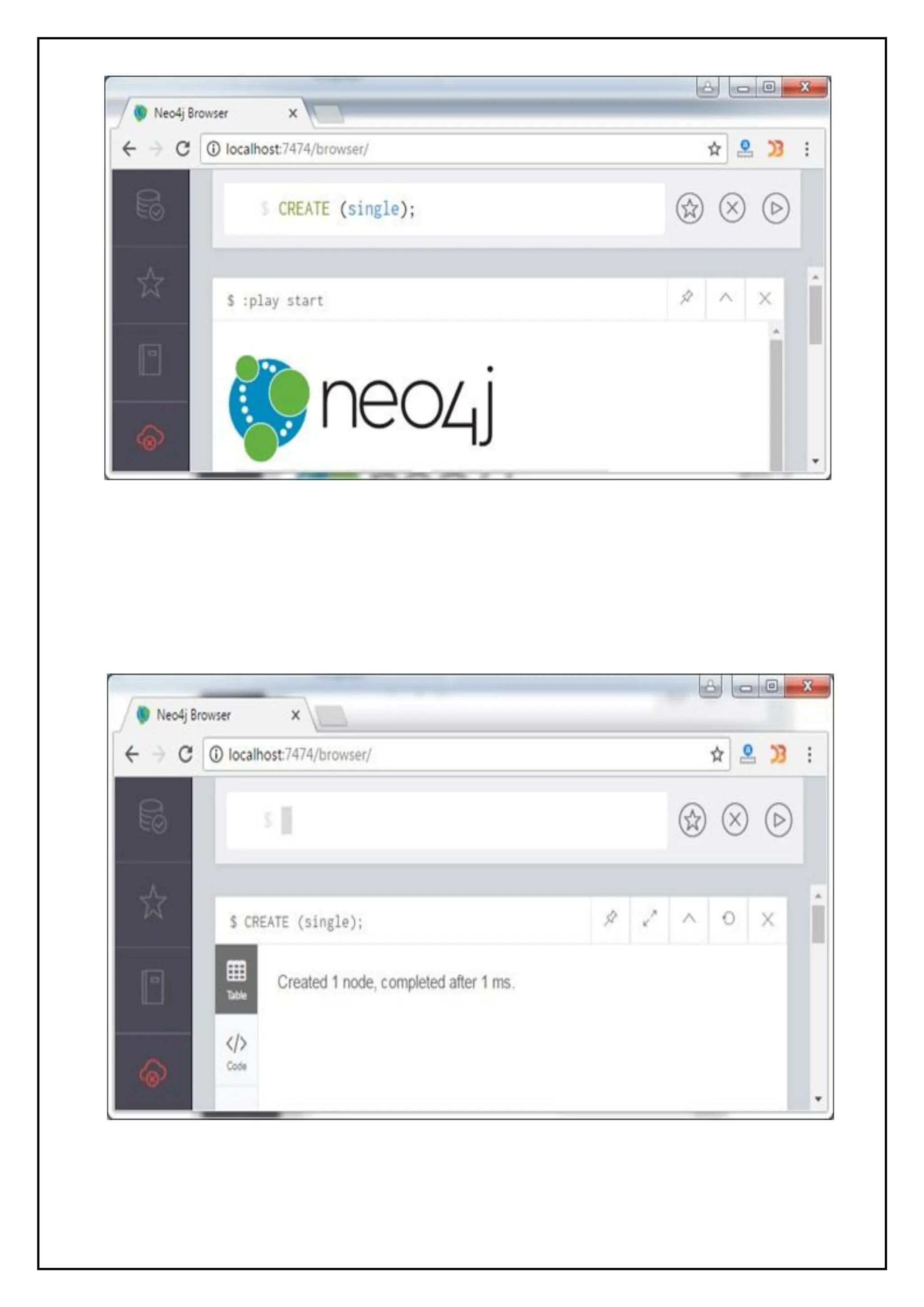
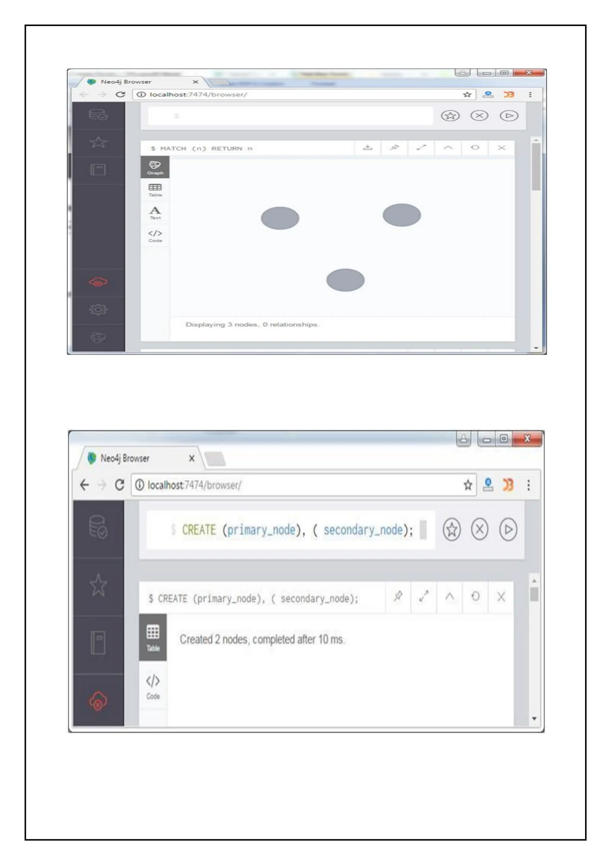
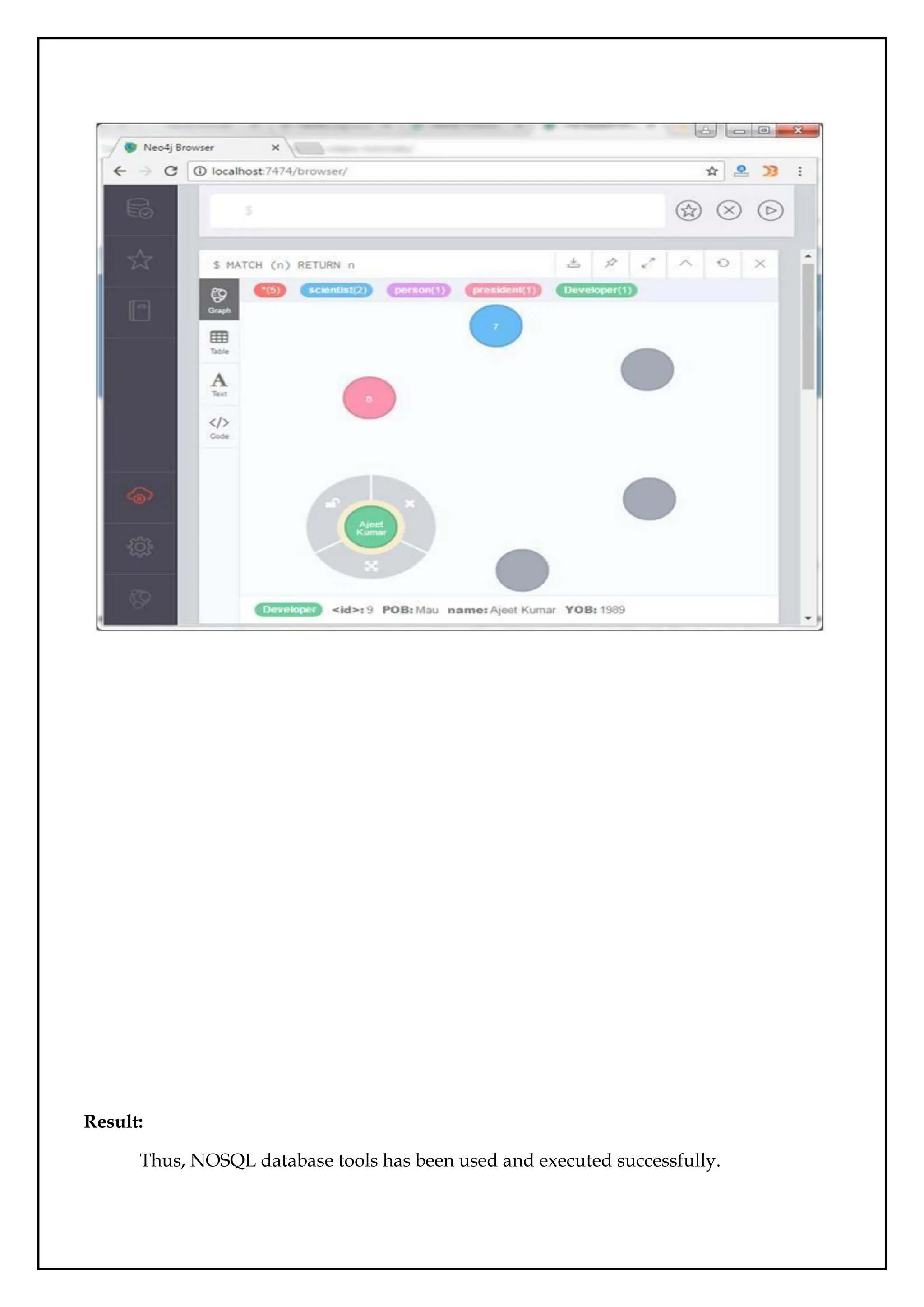
NOSQL
Date:
Aim:
To create document,column and graph based data using NOSQL database tools.
Description:
NoSQL is an umbrella term to describe any alternative system to traditional SQL
databases.
NoSQL databases are all quite different from SQL databases. They use a data model
that has a different structure than the traditional row-and-column table model used with
relational database management systems (RDBMS).
The four main types of NoSQL databases:
1. Document databases
2. Key-value stores
3. Column-oriented databases
4. Graph databases
Document Databases:
A document database stores data in JSON, BSON, or XML documents (not Word
documents or Google Docs, of course). In a document database, documents can be nested.
Particular elements can be indexed for faster querying.
Documents can be stored and retrieved in a form that is much closer to the data
objects used in applications, which means less translation is required to use the data in an
application. SQL data must often be assembled and disassembled when moving back and
forth between applications and storage.
Use cases include ecommerce platforms, trading platforms, and mobile app
development across industries.
Key-value stores
The simplest type of NoSQL database is a key-value store. Every data element in the
database is stored as a key value pair consisting of an attribute name (or "key") and a value.
In a sense, a key-value store is like a relational database with only two columns: the key or
attribute name (such as "state") and the value (such as "Alaska").
Use cases include shopping carts, user preferences, and user profiles.
59.
Column-oriented databases:
While arelational database stores data in rows and reads data row by row, a column
store is organized as a set of columns. This means that when you want to run analytics on a
small number of columns, you can read those columns directly without consuming memory
with the unwanted data. Columns are often of the same type and benefit from more efficient
compression, making reads even faster. Columnar databases can quickly aggregate the value
of a given column (adding up the total sales for the year, for example). Use cases include
analytics.
Unfortunately, there is no free lunch, which means that while columnar databases are
great for analytics, the way in which they write data makes it very difficult for them to be
strongly consistent as writes of all the columns require multiple write events on disk.
Relational databases don't suffer from this problem as row data is written contiguously to
disk.
Graph databases:
A graph database focuses on the relationship between data elements. Each element is
stored as a node (such as a person in a social media graph). The connections between
elements are called links or relationships. In a graph database, connections are first-class
elements of the database, stored directly. In relational databases, links are implied, using
data to express the relationships.
A graph database is optimized to capture and search the connections between data
elements, overcoming the overhead associated with JOINing multiple tables in SQL.
Very few real-world business systems can survive solely on graph queries. As a result
graph databases are usually run alongside other more traditional databases.
Use cases include fraud detection, social networks, and knowledge graphs.
Create Database:
>use javatpointdb
Swithched to db javatpointdb
>db
Check the Database:
>show dbs
local 0 local 0.078GB
Insert a document:
>db.movie.insert({"name":"javatpoint"})
db.javatpoint.insert(
Ex.No.:12
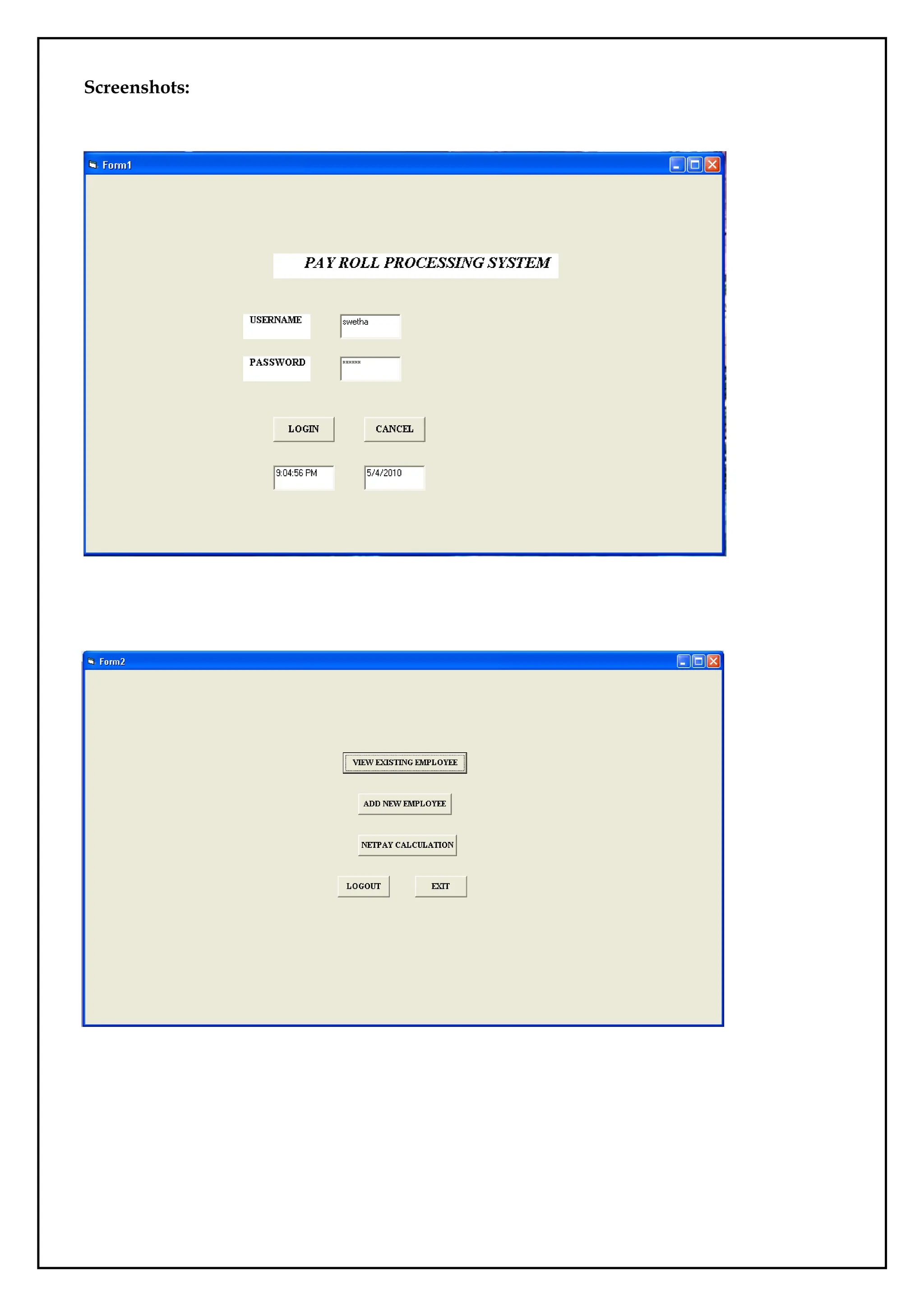
GUI based databaseapplication-Payroll processing System
Date:
Aim:
To develop a payroll processing system in GUI based database.
Description:
This says about the Payroll Processing System and gives the details of an employee in
an organization. The task of this system is to view the details of the particular employee,
adding of new employee to the database and calculates the net pay of each employee.
Microsoft Visual Basic is used as front end and the Oracle as the back end. The visual basic
and the oracle are connected using the component controls such as Microsoft ADO Data
Control 6.0 and Microsoft DataGrid control.
Database Design:
Create the database with the following fields.
FIELDNAME DATATYPE WIDTH
Emp_id Number 5
Name Varchar 15
Age Number 2
Designation Varchar 15
Basicpay Number 7
HRA Number 5
DA Number 5
PF Number 5
Coding:
LOGIN FORM:
Private Sub Command1_Click()
If Text1.Text = "swetha" And Text2.Text = "swetha" Then
Form2.Show
Form1.Hide
Else
MsgBox ("Invalid")
65.
End If
Text1.Text =" "
Text2.Text = " "
End Sub
Private Sub Command2_Click()
End
End Sub
Private Sub Form_Load()
Text3.Text = Time
Text4.Text = Date
End Sub
HOME PAGE FORM:
Private Sub Command1_Click()
Form2.Hide
Form4.Show
End Sub
Private Sub Command2_Click()
Form2.Hide
Form3.Show
End Sub
Private Sub Command3_Click()
Form2.Hide
Form5.Show
End Sub
66.
Private Sub Command4_Click()
Form2.Hide
Form1.Show
EndSub
Private Sub Command5_Click()
End
End Sub
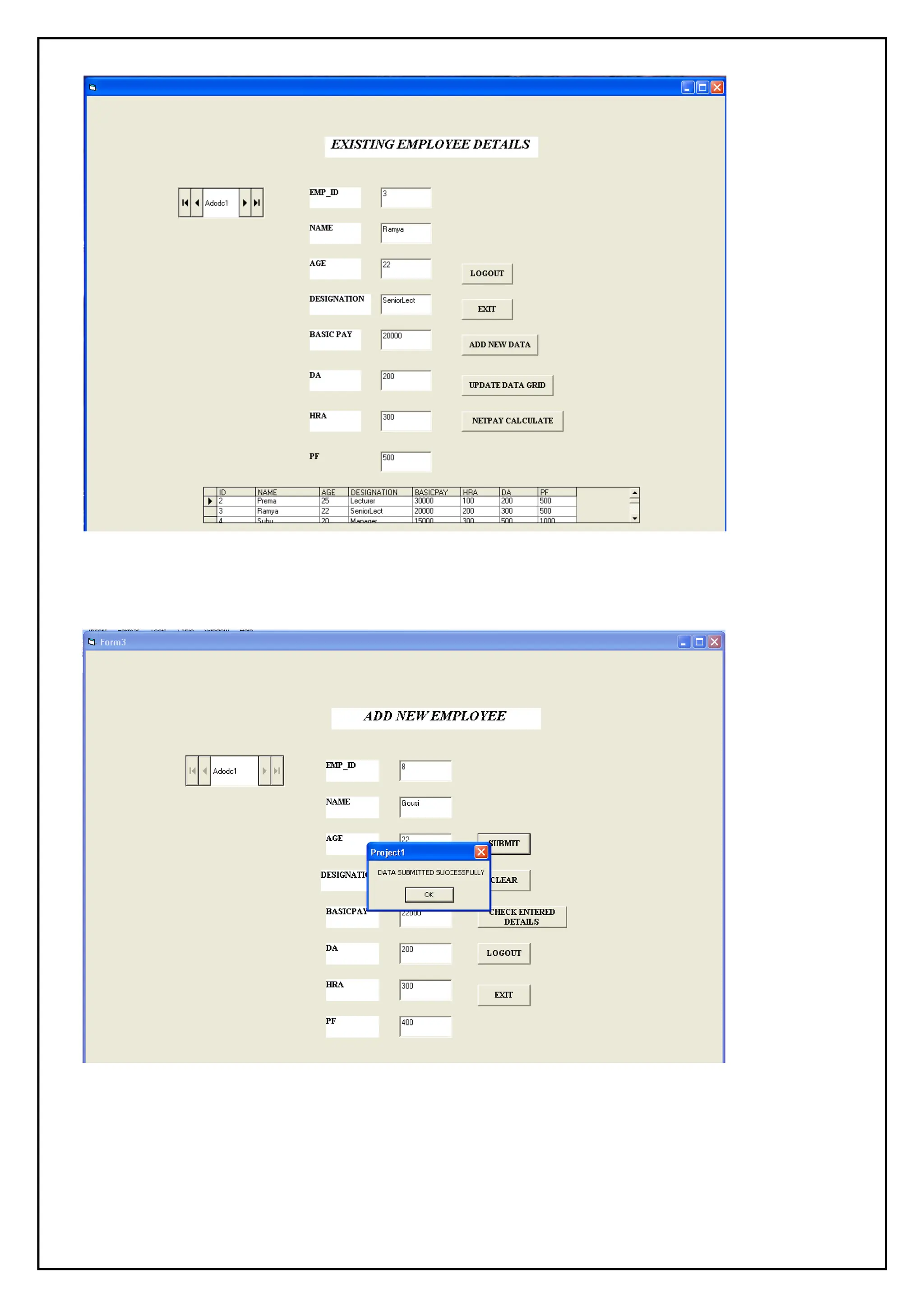
NEW EMPLOYEE FORM:
Dim query1 As New ADODB.Recordset
Dim guideconn1 As New ADODB.Connection
Private Sub Command1_Click()
guideconn1.ConnectionString = "Provider=MSDAORA.1; Password=chellam; User
ID=system;Persist Security Info=false"
guideconn1.Open
Set query1 = guideconn1.Execute("insert into emps12 values('" & (Text1.Text) & "','" &
(Text2.Text) & "','" & (Text3.Text) & "','" & (Text4.Text) & "','" & (Text5.Text) & "','" &
(Text6.Text) & "','" & (Text7.Text) & "','" & (Text8.Text) & "')")
guideconn1.Close
MsgBox ("DATA SUBMITTED SUCCESSFULLY")
End Sub
Private Sub Command2_Click()
Text1.Text = " "
Text2.Text = " "
Text3.Text = " "
Text4.Text = " "
Text5.Text = " "
67.
Text6.Text = ""
Text7.Text = " "
Text8.Text = " "
End Sub
Private Sub Command3_Click()
Form3.Hide
Form4.Show
End Sub
Private Sub Command4_Click()
Form3.Hide
Form1.Show
End Sub
Private Sub Command5_Click()
End
End Sub
EXISTING EMPLOYEE FORM:
Private Sub Command1_Click()
Form4.Hide
Form1.Show
End Sub
Private Sub Command2_Click()
End
End Sub
68.
Private Sub Command3_Click()
Form4.Hide
Form3.Show
EndSub
Private Sub Command4_Click()
Adodc1.CommandType = adCmdText
Adodc1.RecordSource = "select * from emps12"
Adodc1.Refresh
DataGrid1.Refresh
End Sub
Private Sub Command5_Click()
Form4.Hide
Form5.Show
End Sub
Private Sub Text1_Change()
End Sub
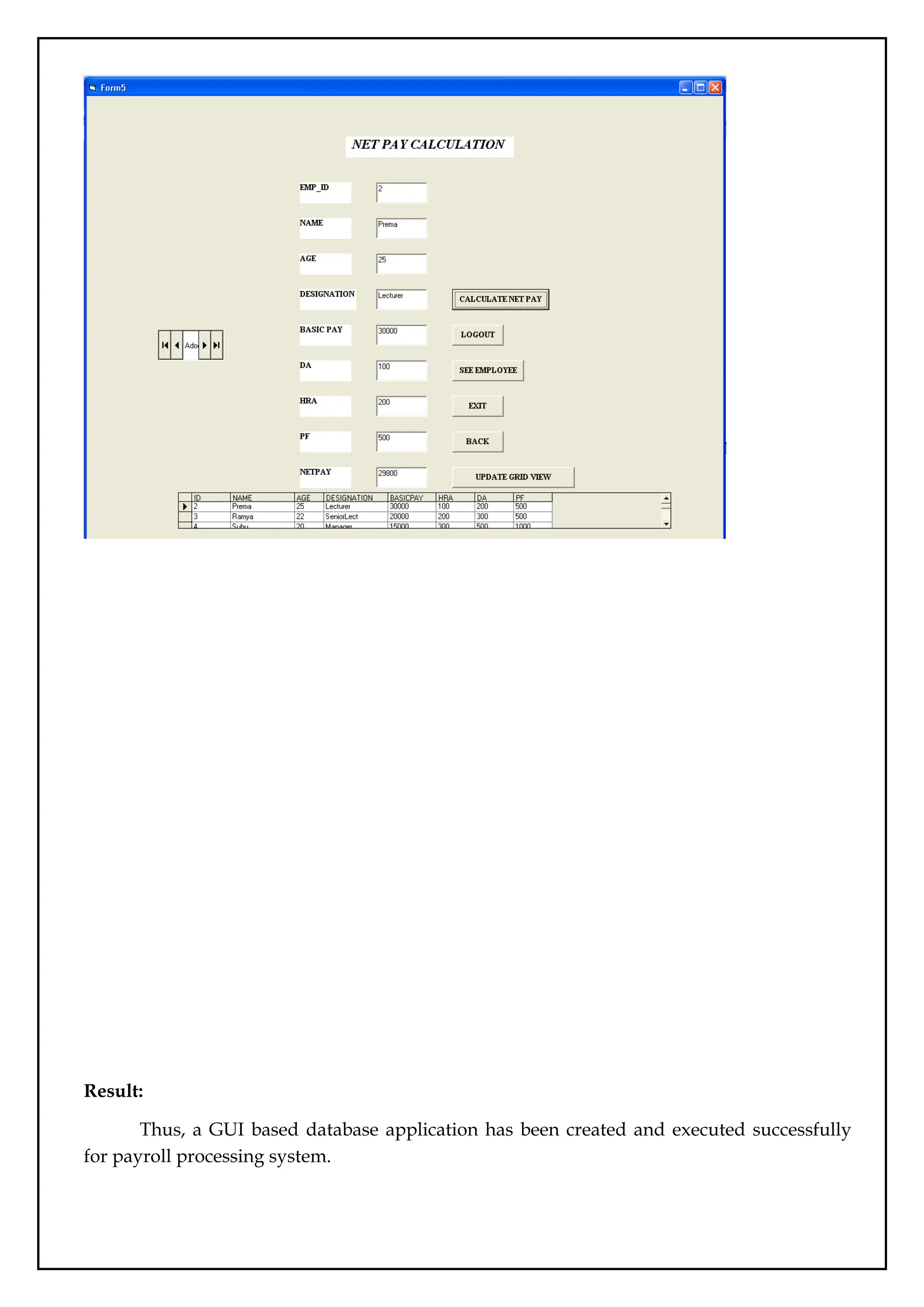
NETPAY CALCULATION FORM:
Dim query As New ADODB.Recordset
Dim guideconn2 As New ADODB.Connection
Private Sub Command1_Click()
Text9.Text = ((Val(Text5.Text) + Val(Text6.Text) + Val(Text7.Text) - Val(Text8.Text)))
End Sub
Private Sub Command2_Click()
69.
Form5.Hide
Form1.Show
End Sub
Private SubCommand3_Click()
Form5.Hide
Form4.Show
End Sub
Private Sub Command4_Click()
End
End Sub
Private Sub Command5_Click()
Form5.Hide
Form2.Show
End Sub
Private Sub Command6_Click()
Adodc1.CommandType = adCmdText
Adodc1.RecordSource = "select * from emps12"
Adodc1.Refresh
DataGrid1.Refresh
End Sub
Result:
Thus, a GUIbased database application has been created and executed successfully
for payroll processing system.
73.
Ex.No.:13
Case Study-EMart GroceryShop
Date:
Aim:
To create a database for Emart Grocery shop and apply all sql properties.
Sample Code:
SQL> create table grocery_visit(date TEXT, time_spent_min INTEGER, amount_spent
REAL);
SQL>create table grocery_list(date TEXT, item_name TEXT, item_category TEXT);
SQL>insert into grocery_list values("2020-12-03", "Hamburger patties", "Meat and
Fish");insert into grocery_list values("2020-12-03", "Chips", "Pantry");
SQL>insert into grocery_list values("2020-12-03", "Avocado", "Fruits and Vegetables"); insert
into grocery_list values("2020-12-03", "Lime", "Fruits and Vegetables"); insert into grocery_list
values("2020-12-03", "Tomato", "Fruits and Vegetables");
SQL>insert into grocery_list values("2020-12-15", "Rice cakes", "Pantry");insert into
grocery_list values("2020-12-15", "Graham crackers", "Pantry");
SQL>insert into grocery_list values("2020-12-15", "Toothpaste", NULL); insert into
grocery_list values("2020-12-15", "Flour", "Pantry"); insert into grocery_list values("2020-12-
15", "Yeast", "Pantry"); insert into grocery_list values("2020-12-15", "Popcorn", "Pantry");
insert into grocery_list values("2020-12-15", "Eggs", NULL);
SQL>insert into grocery_list values("2020-12-15", "Milk", "Dairy");
SQL>insert into grocery_list values("2020-12-15", "Bananas", "Fruits and Vegetables");insert
into grocery_list values("2020-12-15", "Frozen waffles", NULL);
SQL>insert into grocery_list values("2020-12-23", "Mayo", "Pantry"); insert into grocery_list
values("2020-12-23", "Flour", "Pantry"); insert into grocery_list values("2020-12-23", "Milk",
"Dairy");
SQL>insert into grocery_list values("2020-12-23", "Roasted Chicken", "Meat and Fish");insert
into grocery_list values("2020-12-23", "Chocolate chip cookies", "Pantry");
SQL>insert into grocery_list values("2020-12-23", "Yogurt", "Dairy"); insert into grocery_list
values("2020-12-23", "Soda", NULL);
74.
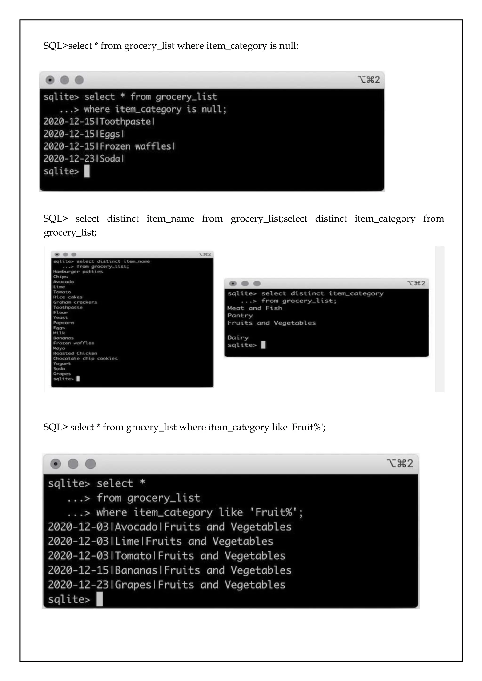
SQL>select * fromgrocery_list where item_category is null;
SQL> select distinct item_name from grocery_list;select distinct item_category from
grocery_list;
SQL> select * from grocery_list where item_category like 'Fruit%';
75.
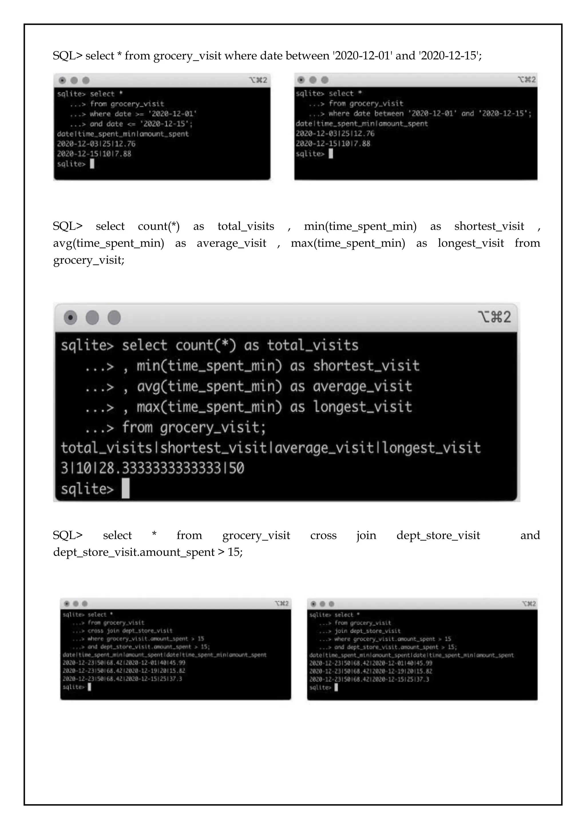
SQL> select *from grocery_visit where date between '2020-12-01' and '2020-12-15';
SQL> select count(*) as total_visits , min(time_spent_min) as shortest_visit ,
avg(time_spent_min) as average_visit , max(time_spent_min) as longest_visit from
grocery_visit;
SQL> select * from grocery_visit cross join dept_store_visit and
dept_store_visit.amount_spent > 15;
CONTENT BEYOND SYLLABUS
DATABASEDESIGN USING ER MODELING, NORMALIZATION AND
IMPLEMENTATION FOR LIBRARY MANAGEMENT SYSTEM
AIM:
To create database design using ER modeling, normalization and implementation for
library management application.
DESCRIPTION:
Project Overview Statement
As you know that a Library is collection of books in any institute. Librarian
responsibility is to manage all the records of books issued and also returned on manually.
Case study
Current system:
All the Transaction (books issues & books returned) are manually recorded (registers.)
Students search books by racks it so time consuming
And there is no arrangement. Also threat of losing recorded.
Project Aim and Objective
The project aim and objective are:
To eliminate the paper –work in library
To record every transaction in computerized system so that problem such as record
file missing won‘t happen again
Backgroud of Project
Library Management system is an application refer to other library system and is
suitable to use by small and medium size libray. It is use by librarian and libray admin to
manage the library using a computerized system.
The system was designed to help librain record every book transcation so that the
problem such as file missing will not happened again.
Design view
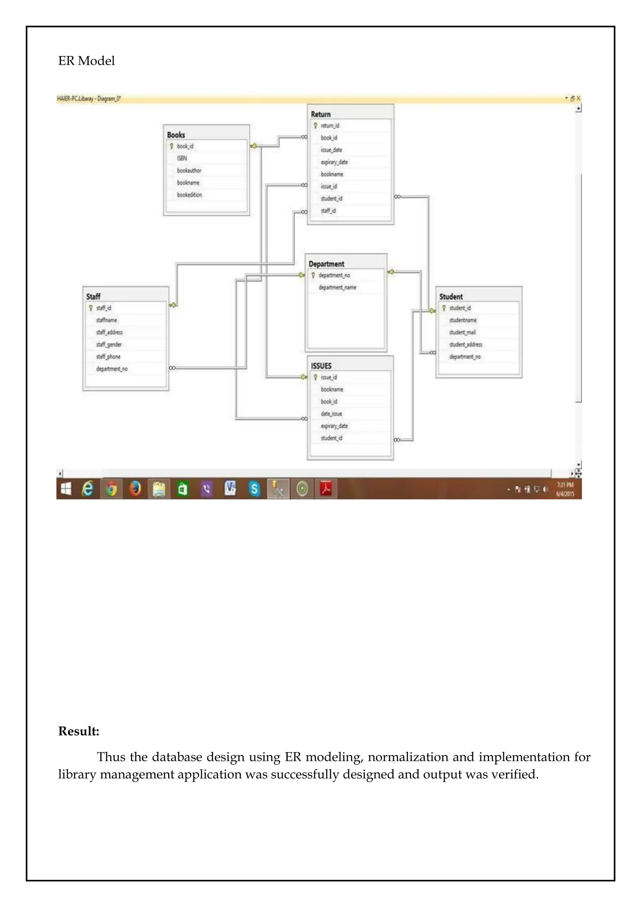
The library has the following tables in its database;
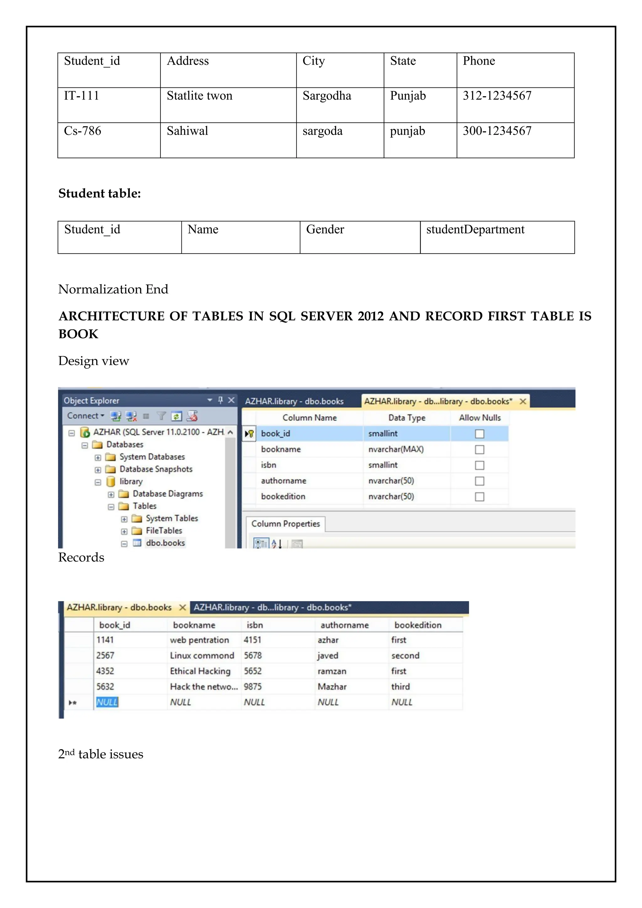
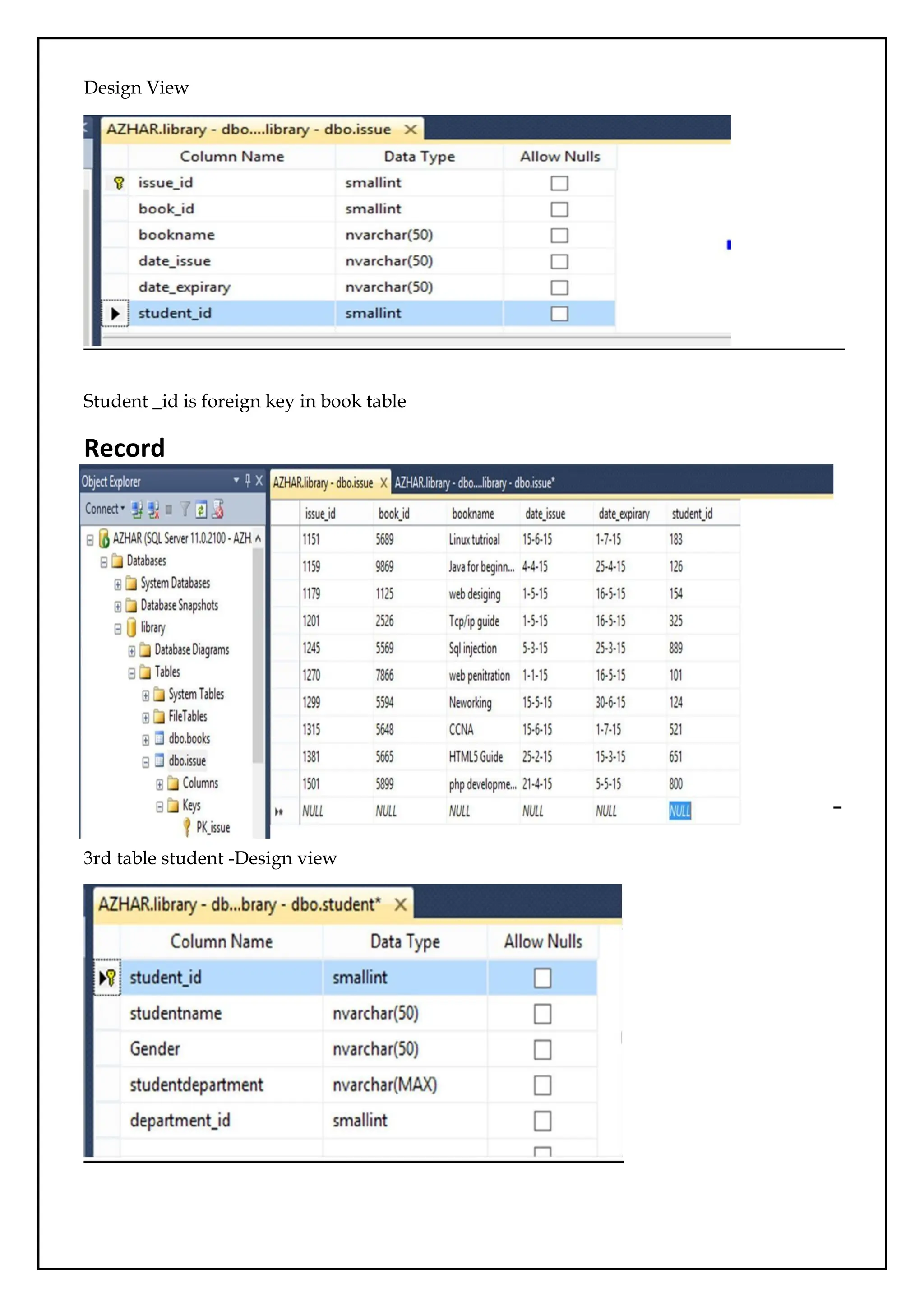
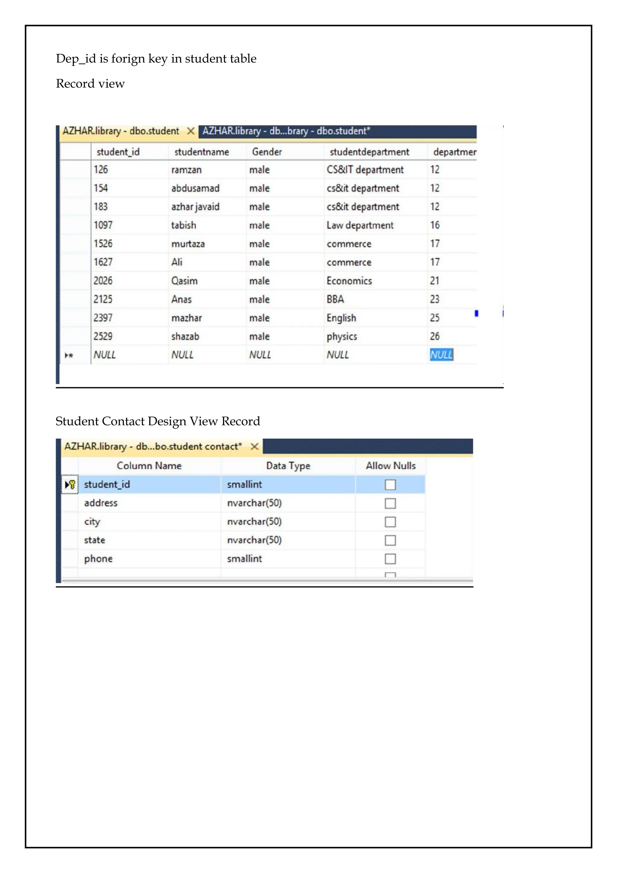
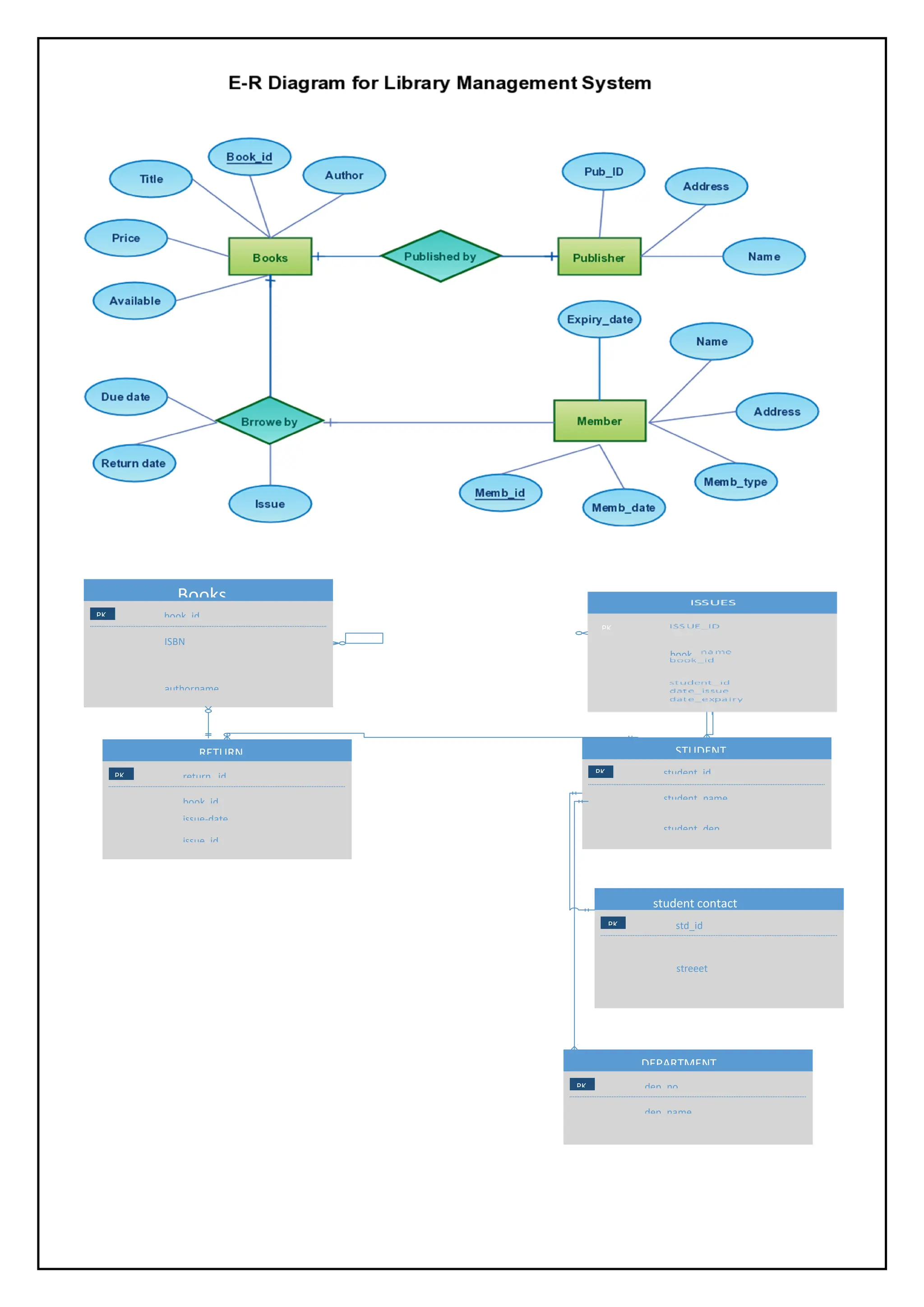
1. Books (book_id, ISBN,bookName, BOOKAUTHOR and bookedition)
2. student (student_id, studentname, student_email, student_address)
3. Staff (staff_id, staff_name, staff_address, staff_gender, staff_phone)
4. department (department_id, branch_name)
78.
5. Issue (issue_id,issue_date, expiry_date, book_name, book_id)
6. Return (return_id, expiry_date, isuue_date, book_id)
NORAMALIZATION OF TABLE
Why Normalization:
Database normalization is the process of removing redundant data from your tables in
order to improve storage efficiency, data integrity, and scalability.
Normalization generally involves splitting existing tables into multiple ones, which
must be re-joined or linked each time a query is issued.
Normalization of Tables in Database
Issue_id Book_id Student_id
1122 110,120,320 bitE183
In the ISSUE Table there is repeating book_id . A student has issued 3 books.
After first Normalization
ISSUE_ID book_id Student_id
1122 110 bitE183
1122 320 bitE183
1122 120 bitE183
Second normalized Form:
In the following Student relation all attributes are dependent on the primary key StudID
Student_id Name Depid Issue_date Expairy_date Phone
BITf13E183 Azhar 20 17-6-15 1-7-15 3127400
We can create two other relations from Student Table one is Department fields are
fully dependent on the primary keys DEp_id
DEp_id Dep_name
11 CS & IT Department
22 Education Department
33 Economics Department
44 Laaw Department
Student_id Name Issue_date Expairy_date Phone
79.
BITf13E183 Azhar 15-6-151-7-15 312-7400558
Before third normal form
Staff_id Name Gender Designation Address City state cell
1101 Shaid M Librarian
House no12
street 6 Sargodha punjab
300-
1234567
1345 Riaz m Data entery
Statilete
town Sargodha Punjab
0346-
1234567
2264 Arshad m Naib qaisd
Raza
garden Sargodha Punjab
0333-
1234567
After 3rd Normalization
Staff table
Staff_id Name Gender
Staff conatact
Staff_id Address City State Telephone cell
STUDENT Table before Third normalized Form :
Student table
Std_id Name Gender Address City State Phone Dep_id
After third normal
Student_id Dep_id Department
IT-113 C-26 Cs & IT
Lm-456 L-11 Law
Eng-98 E-41 ENGLISH
Studentcontact table:
80.
Student_id Address CityState Phone
IT-111 Statlite twon Sargodha Punjab 312-1234567
Cs-786 Sahiwal sargoda punjab 300-1234567
Student table:
Normalization End
ARCHITECTURE OF TABLES IN SQL SERVER 2012 AND RECORD FIRST TABLE IS
BOOK
Design view
Records
2nd table issues
Student_id Name Gender studentDepartment
ER Model
Result:
Thus thedatabase design using ER modeling, normalization and implementation for
library management application was successfully designed and output was verified.


![To drop columns in a table:
ALTER TABLE table_name DROP COLUMN column_name;
To rename a column in a table:
ALTER TABLE table_name RENAME COLUMN old_name to new_name;
4. TRUNCATE: This is used to remove all records from a table, including all spaces
allocated for the records are removed.
Syntax: TRUNCATE TABLE table_name;
5. COMMENT: This is used to add comments to the data dictionary.
6. RENAME: This is used to rename an object existing in the database.
Syntax: ALTER TABLE table_name RENAME TO new_table_name;
DML - Data Manipulation Language
The SQL commands that deals with the manipulation of data present in the database belong
to DML or Data Manipulation Language and this includes most of the SQL statements. It is
the component of the SQL statement that controls access to data and to the database.
Basically, DCL statements are grouped with DML statements.
List of DML commands:
1. INSERT: It is used to insert data into a table.
Syntax: INSERT INTO TABLE_NAME (col1, col2, col3,.... col N) VALUES (value1,
value2, value3, .... valueN);
Or
INSERT INTO TABLE_NAME
VALUES (value1, value2, value3, .... valueN);
2. UPDATE: It is used to update existing data within a table.
Syntax: UPDATE table_name SET [column_name1= value1,...column_nameN =
valueN] [WHERE CONDITION]
3. DELETE: It is used to delete records from a database table.
Syntax: DELETE FROM table_name [WHERE condition];
SQL Constraints
SQL constraints are used to specify rules for the data in a table.Constraints are used to
limit the type of data that can go into a table. This ensures the accuracy and reliability of the
data in the table. If there is any violation between the constraint and the data action, the
action is aborted.
Constraints can be column level or table level. Column level constraints apply to a
column, and table level constraints apply to the whole table.](https://image.slidesharecdn.com/databasemanagementlab-250424094923-0c8b9987/75/CS3481_Database-Management-Laboratory-pdf-8-2048.jpg)
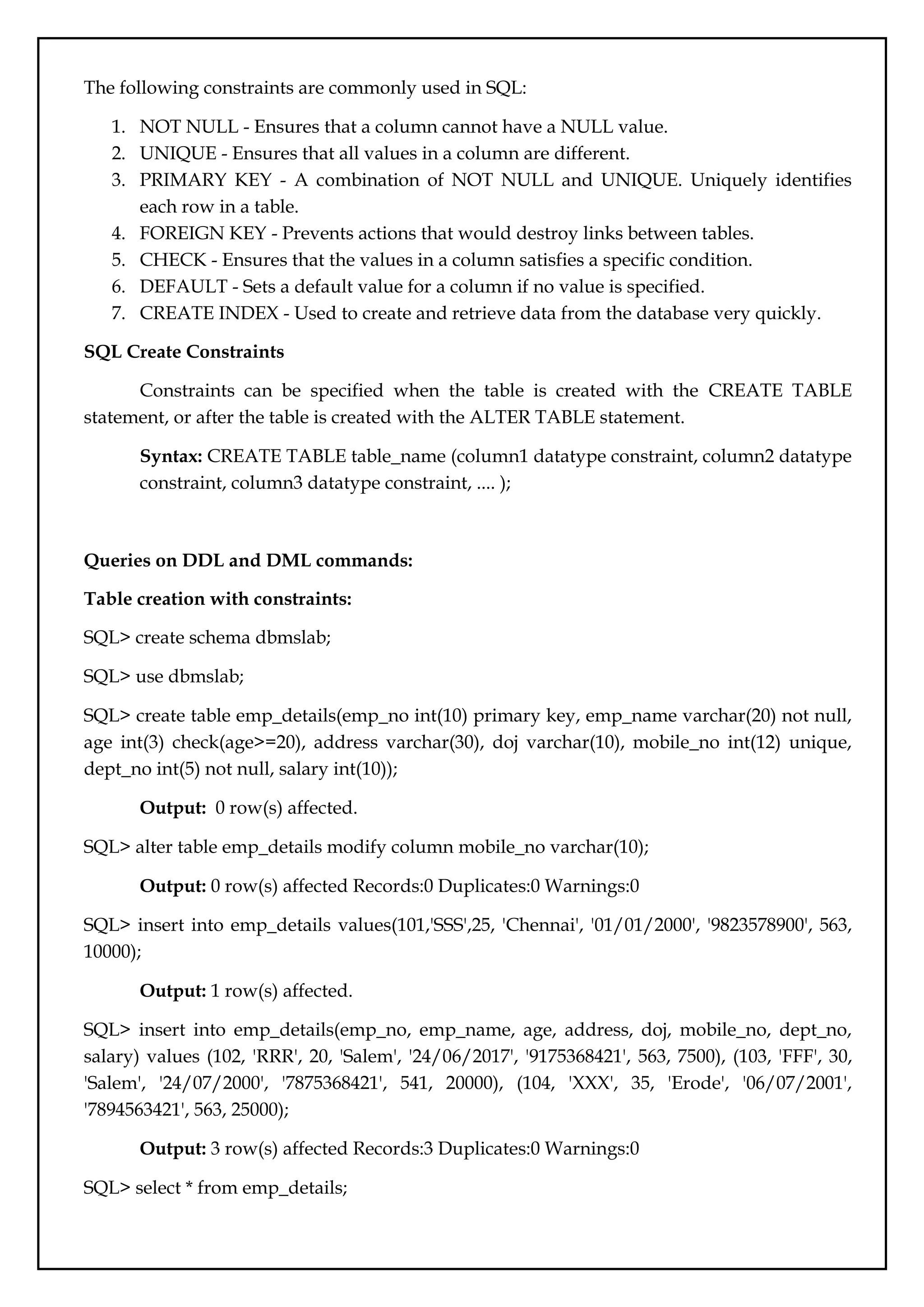
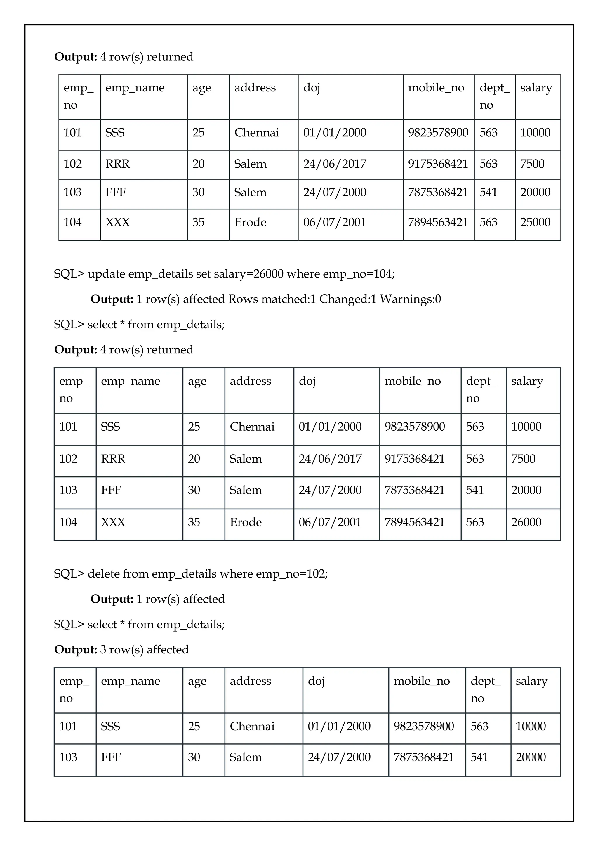
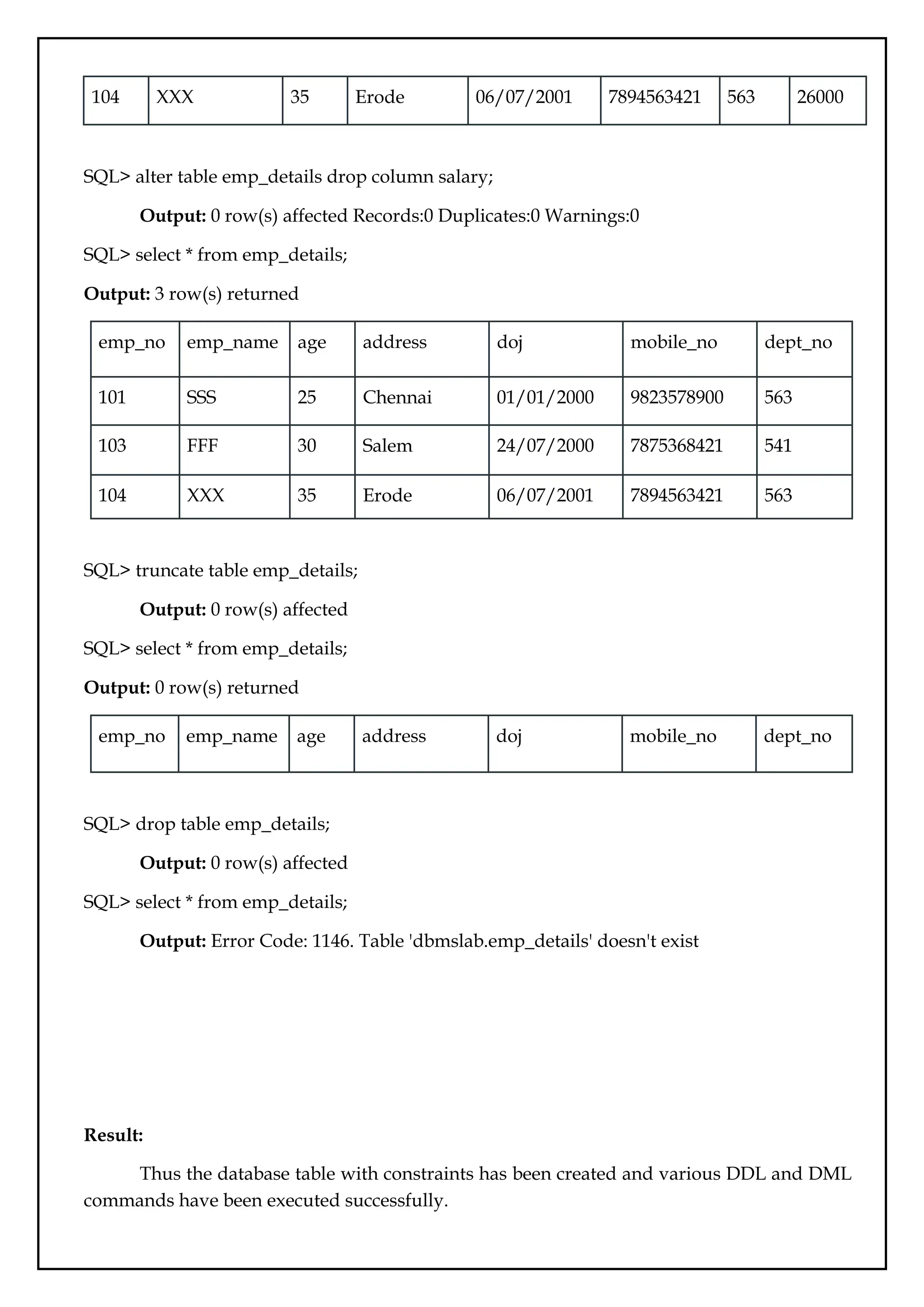
![Ex.No.:02
Referential Integrity
Date:
Aim:
To create a set of tables, add foreign key constraints and incorporate referential
integrity.
Description:
Referential integrity refers to the relationship between tables. Because each table in a
database must have a primary key, this primary key can appear in other tables because of its
relationship to data within those tables. When a primary key from one table appears in
another table, it is called a foreign key.
The table containing the foreign key is called the child table(Referencing Table), and
the table containing the Primary key/candidate key is called the master or parent
table(Referenced Table).
The essential syntax for a defining a foreign key constraint in a CREATE TABLE or
ALTER TABLE statement includes the following:
Syntax: [CONSTRAINT [symbol]] FOREIGN KEY [index_name] (col_name, ...)
REFERENCES tbl_name (col_name,...) [ON DELETE reference_option] [ON UPDATE
reference_option]
reference_option:
RESTRICT | CASCADE | SET NULL | NO ACTION | SET DEFAULT
Referential Actions
When an UPDATE or DELETE operation affects a key value in the parent table that
has matching rows in the child table, the result depends on the referential action specified by
ON UPDATE and ON DELETE subclauses of the FOREIGN KEY clause.
Referential actions include:
CASCADE: Delete or update the row from the parent table and automatically delete or
update the matching rows in the child table. Both ON DELETE CASCADE and ON UPDATE
CASCADE are supported. Between two tables, do not define several ON UPDATE
CASCADE clauses that act on the same column in the parent table or in the child table.
If an ON UPDATE CASCADE or ON DELETE CASCADE subclause is only defined
for one FOREIGN KEY clause, cascading operations fail with an error.
Note:Cascaded foreign key actions do not activate triggers.](https://image.slidesharecdn.com/databasemanagementlab-250424094923-0c8b9987/75/CS3481_Database-Management-Laboratory-pdf-12-2048.jpg)
![SET NULL: Delete or update the row from the parent table and set the foreign key column or
columns in the child table to NULL. Both ON DELETE SET NULL and ON UPDATE SET
NULL clauses are supported.
RESTRICT: Rejects the delete or update operation for the parent table. Specifying RESTRICT
(or NO ACTION) is the same as omitting the ON DELETE or ON UPDATE clause.
NO ACTION: A keyword from standard SQL. In MySQL, equivalent to RESTRICT. Some
database systems have deferred checks, and NO ACTION is a deferred check. In MySQL,
foreign key constraints are checked immediately, so NO ACTION is the same as RESTRICT.
SET DEFAULT: This action is recognized by the MySQL parser, but both InnoDB and NDB
reject table definitions containing ON DELETE SET DEFAULT or ON UPDATE SET
DEFAULT clauses.
For storage engines that support foreign keys, MySQL rejects any INSERT or
UPDATE operation that attempts to create a foreign key value in a child table if there is no
matching candidate key value in the parent table.
For an ON DELETE or ON UPDATE that is not specified, the default action is always
NO ACTION.
Adding Foreign Key Constraints
A foreign key constraint can be added to an existing table using ALTER TABLE
syntax:
Syntax: ALTER TABLE tbl_name ADD [CONSTRAINT [symbol]] FOREIGN KEY
[index_name] (col_name, ...) REFERENCES tbl_name (col_name,...) [ON DELETE
reference_option] [ON UPDATE reference_option];
Dropping Foreign Key Constraints
A foreign key constraint can be dropped using ALTER TABLE syntax:
Syntax: ALTER TABLE tbl_name DROP FOREIGN KEY fk_symbol;
Queries:
SQL> create table product (category int not null, id int not null, price decimal, primary
key(category, id));
Output: 0 row(s) affected
SQL> create table customer (id int not null, primary key(id));
Output: 0 row(s) affected
SQL> create table product_order (no int not null auto_increment, product_category int not
null, product_id int not null, customer_id int not null, primary key(no), index
(product_category, product_id), index (customer_id), foreign key (product_category,](https://image.slidesharecdn.com/databasemanagementlab-250424094923-0c8b9987/75/CS3481_Database-Management-Laboratory-pdf-13-2048.jpg)
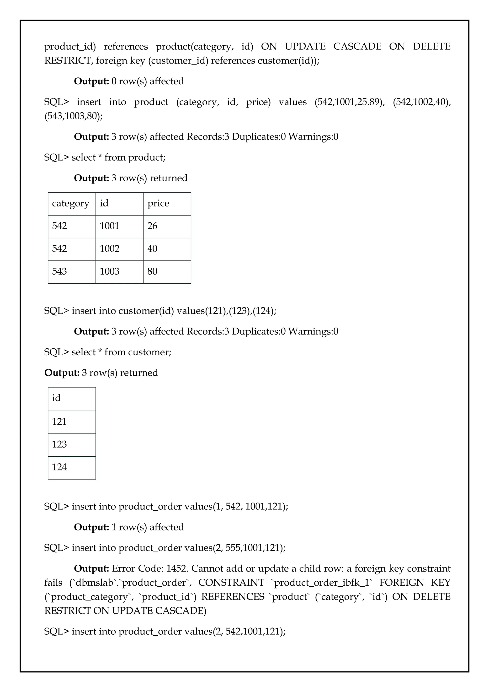
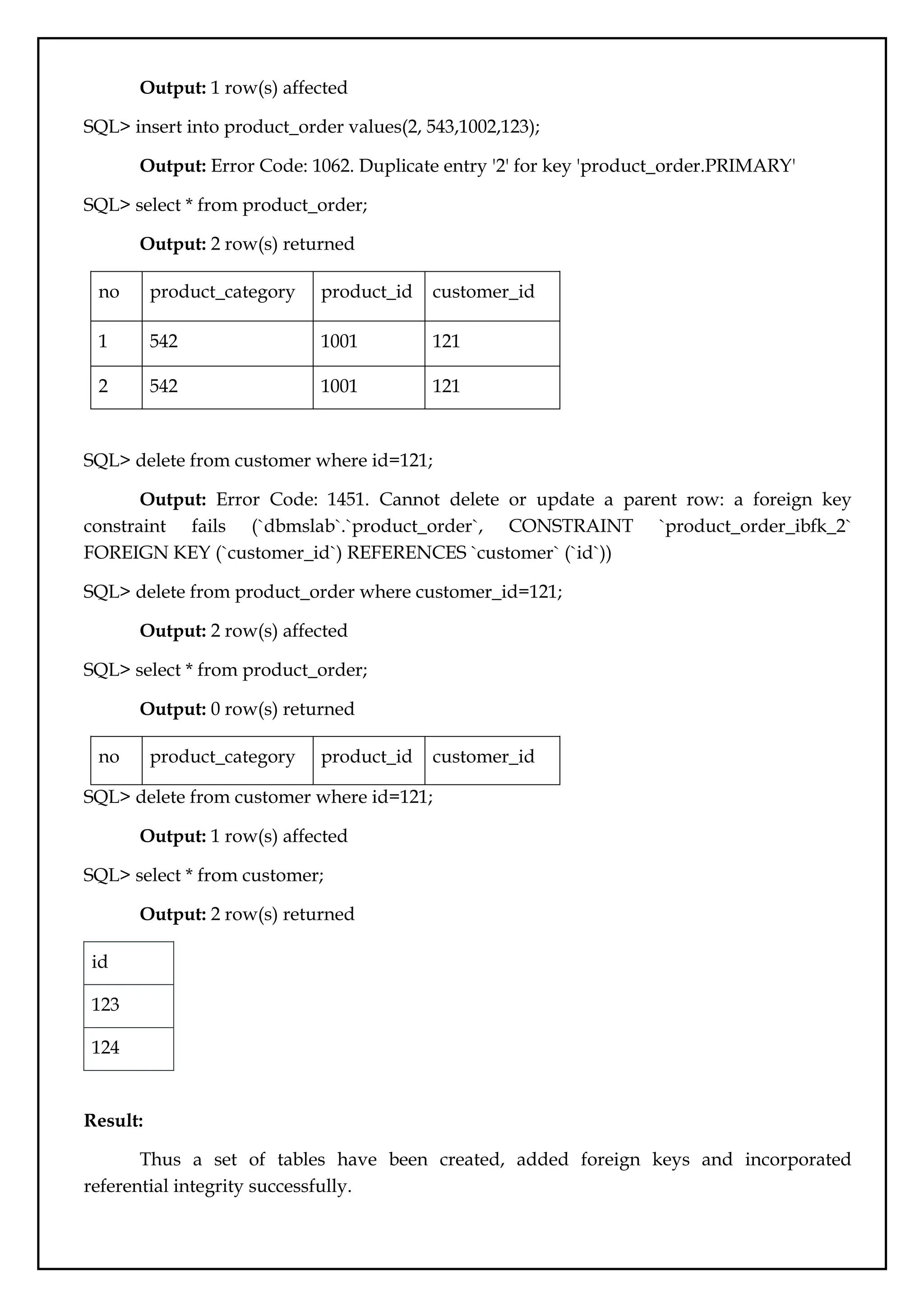
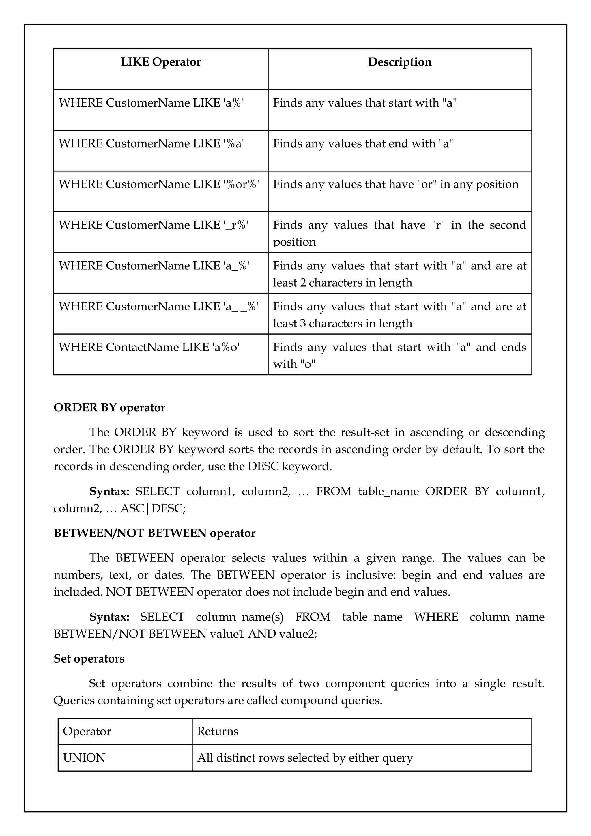
![UNION ALL All rows selected by either query, including all duplicates
INTERSECT All distinct rows selected by both queries
MINUS/EXCEPT All distinct rows selected by the first query but not the second
AND, OR, NOT operators
The WHERE clause can be combined with AND, OR, and NOT operators.
The AND and OR operators are used to filter records based on more than one
condition:
● The AND operator displays a record if all the conditions separated by AND are TRUE.
● The OR operator displays a record if any of the conditions separated by OR is TRUE.
● The NOT operator displays a record if the condition(s) is NOT TRUE.
AND Syntax : SELECT column1, column2, … FROM table_name WHERE condition1
AND condition2 AND condition3 ...;
OR Syntax : SELECT column1, column2, … FROM table_name WHERE condition1
OR condition2 OR condition3 ...;
NOT Syntax : SELECT column1, column2, … FROM table_name WHERE NOT
condition;
Aggregate Function: An aggregate function is a function where the values of multiple rows
are grouped together as input on certain criteria to form a single value of more significant
meaning. Aggregate functions are often used with the GROUP BY and HAVING clauses of
the SELECT statement.
All the aggregate functions are used in the Select statement.
Syntax: SELECT <FUNCTION NAME> (<PARAMETER>) FROM <TABLE NAME>
Common aggregate functions are as follows:
1. COUNT(): The count function returns the number of rows in the result. It does not
count the null values.
Types
COUNT(*): Counts all the number of rows of the table including null.
COUNT( COLUMN_NAME): count number of non-null values in column.
COUNT( DISTINCT COLUMN_NAME): count number of distinct values in a column.
Syntax : COUNT() or COUNT([ALL|DISTINCT] expression)](https://image.slidesharecdn.com/databasemanagementlab-250424094923-0c8b9987/75/CS3481_Database-Management-Laboratory-pdf-18-2048.jpg)
![2. AVG(): The AVG function is used to calculate the average value of the numeric type.
AVG function returns the average of all non-Null values.
Syntax: AVG() or AVG( [ALL|DISTINCT] expression )
3. MIN(): MIN function is used to find the minimum value of a certain column. This
function determines the smallest value of all selected values of a column.
Syntax: MIN() or MIN( [ALL|DISTINCT] expression )
4. MAX(): MAX function is used to find the maximum value of a certain column. This
function determines the largest value of all selected values of a column.
Syntax: MAX() or MAX( [ALL|DISTINCT] expression )
5. SUM(): Sum function is used to calculate the sum of all selected columns. It works on
numeric fields only.
Syntax: SUM() or SUM( [ALL|DISTINCT] expression )
Aggregation with GROUP BY
The GROUP BY statement groups rows that have the same values.
Syntax : SELECT column_name(s) FROM table_name WHERE condition
GROUP BY column_name(s);
HAVING clause
The HAVING clause was added to SQL because the WHERE keyword cannot be used
with aggregate functions.
Syntax : SELECT column_name(s) FROM table_name WHERE condition GROUP BY
column_name(s) HAVING condition;
Queries:
Sample table: PRODUCT_MAST
PRODUCT COMPANY QTY RATE COST
Item1 Com1 2 10 20
Item2 Com2 3 25 75
Item3 Com1 2 30 60
Item4 Com3 5 10 50
Item5 Com2 2 20 40
Item6 Com1 3 25 75](https://image.slidesharecdn.com/databasemanagementlab-250424094923-0c8b9987/75/CS3481_Database-Management-Laboratory-pdf-19-2048.jpg)
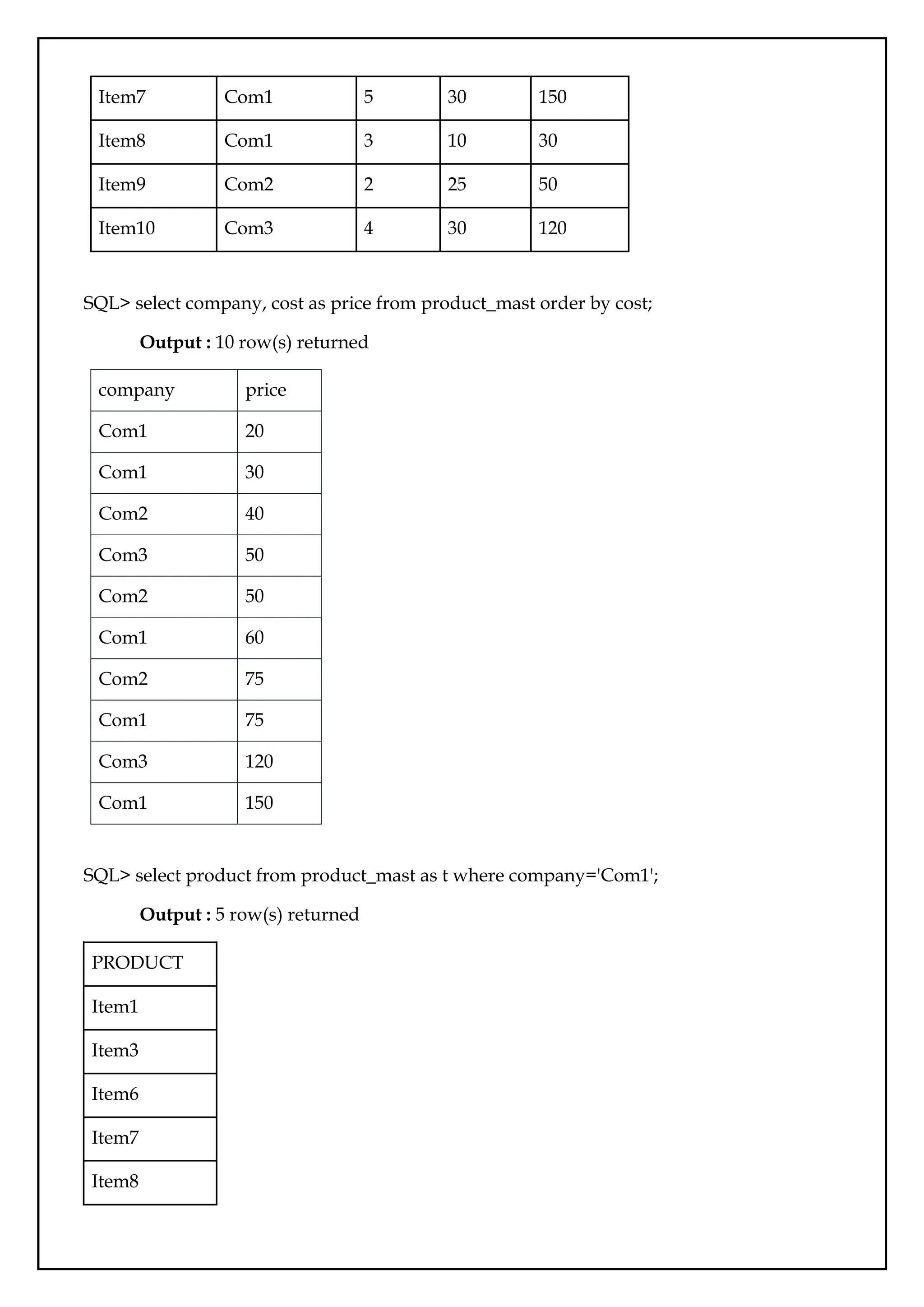
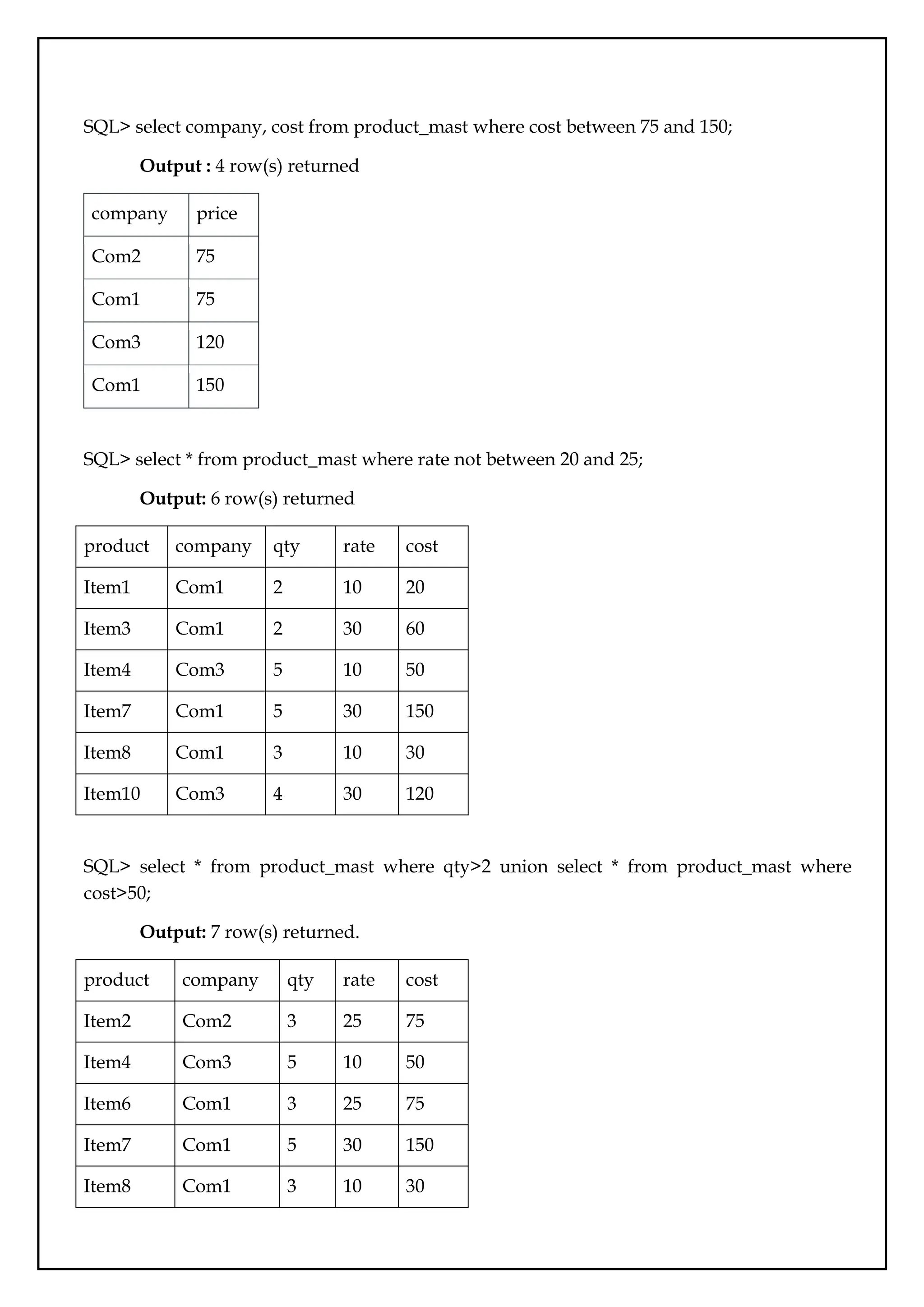
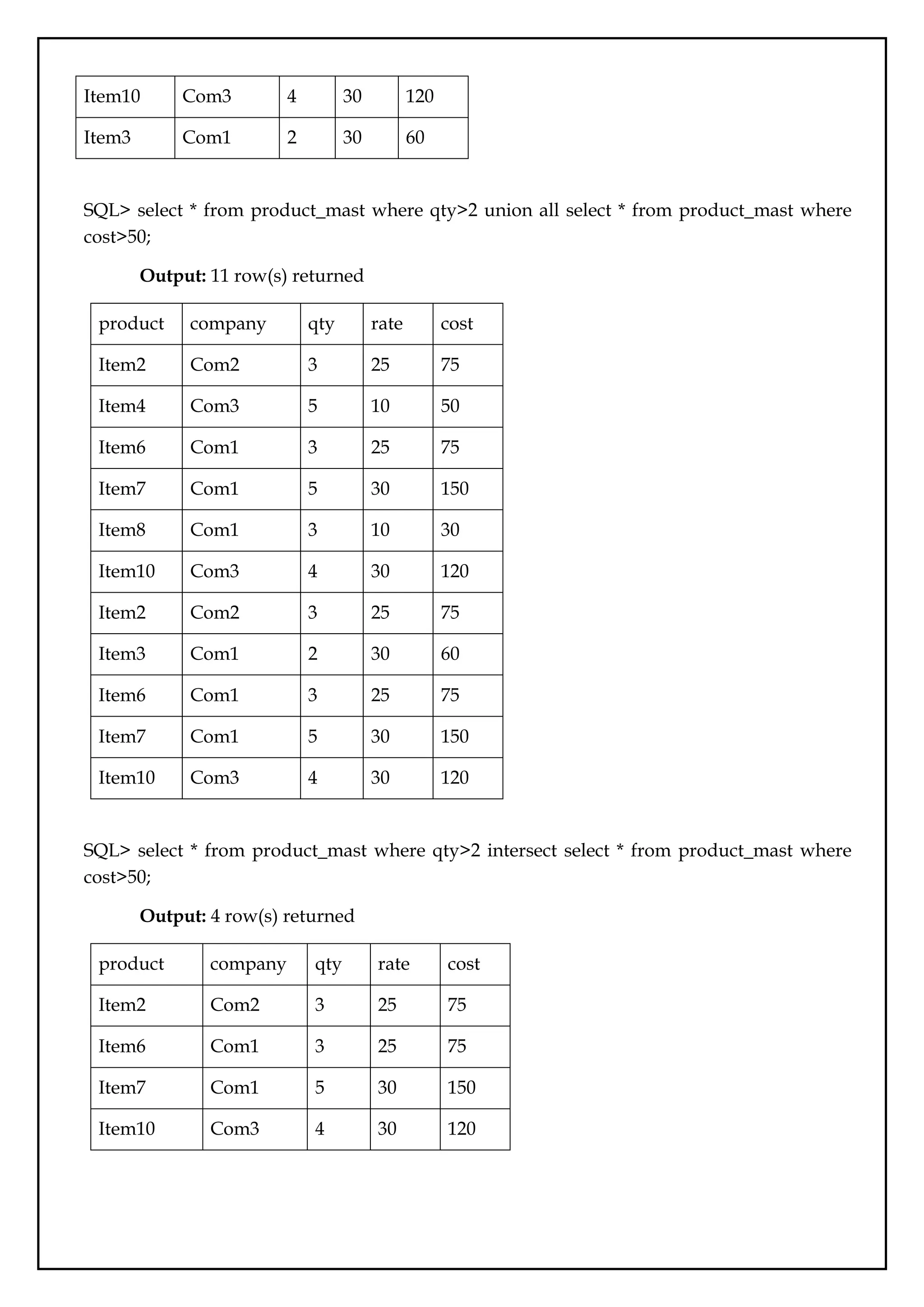
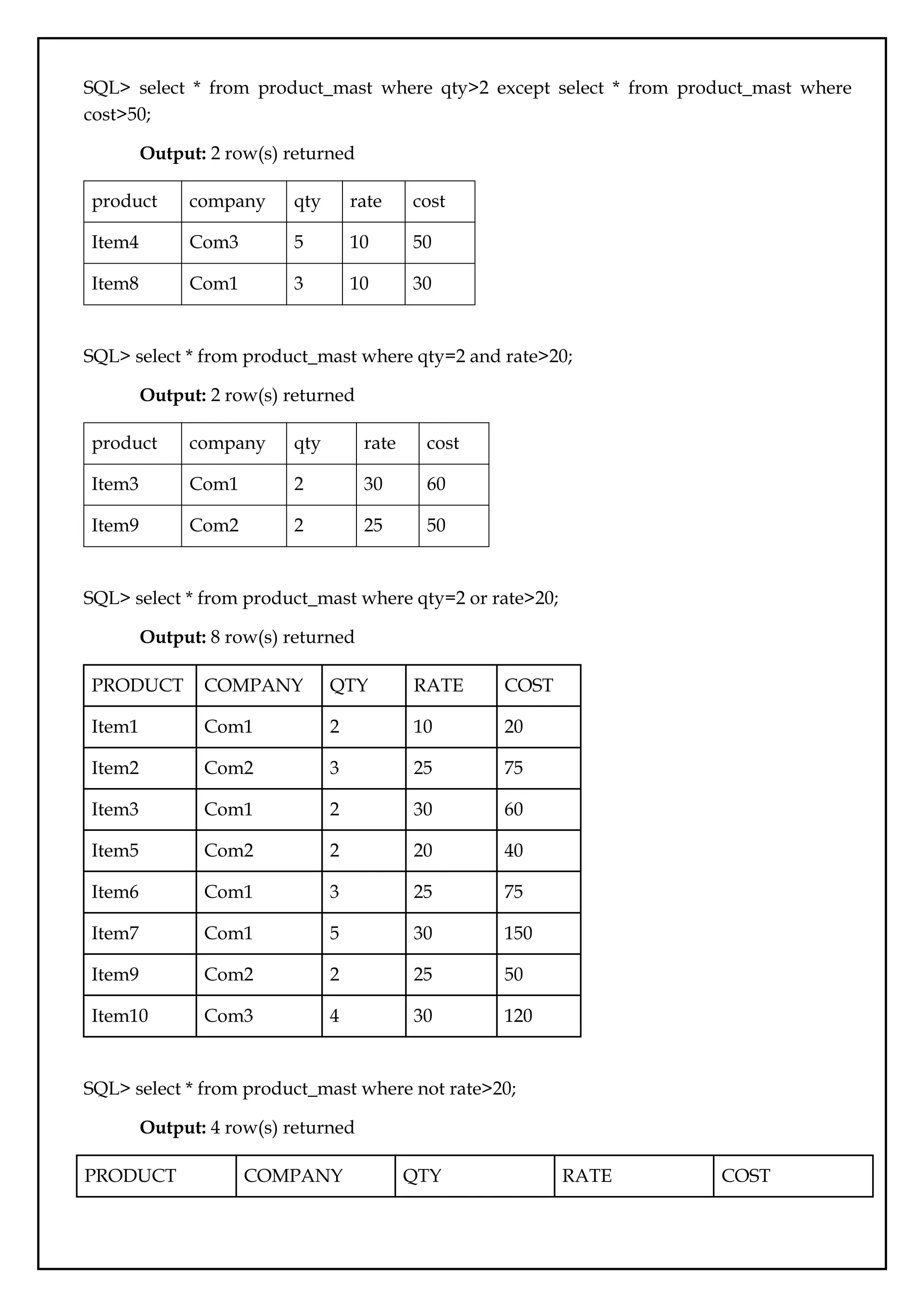
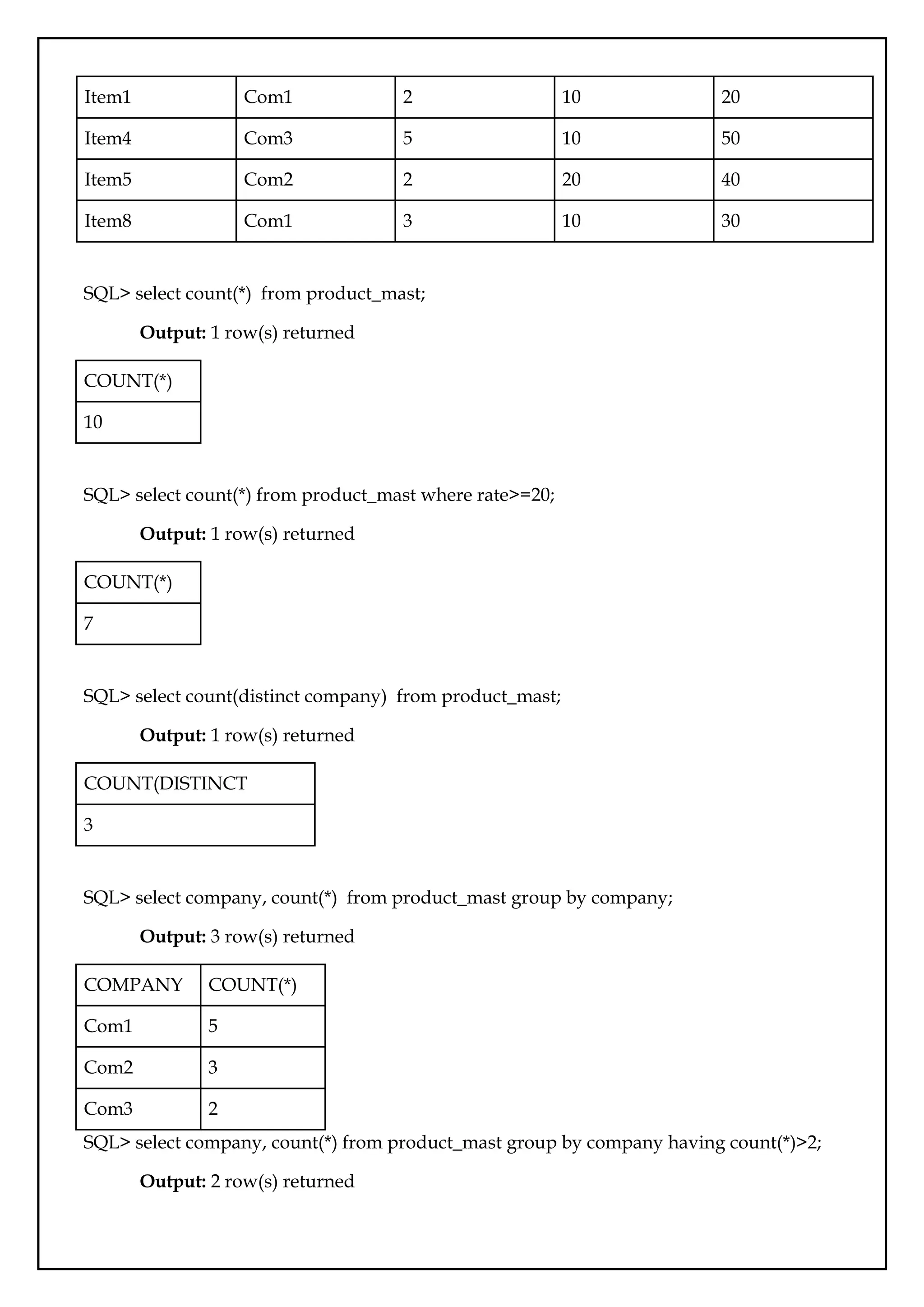
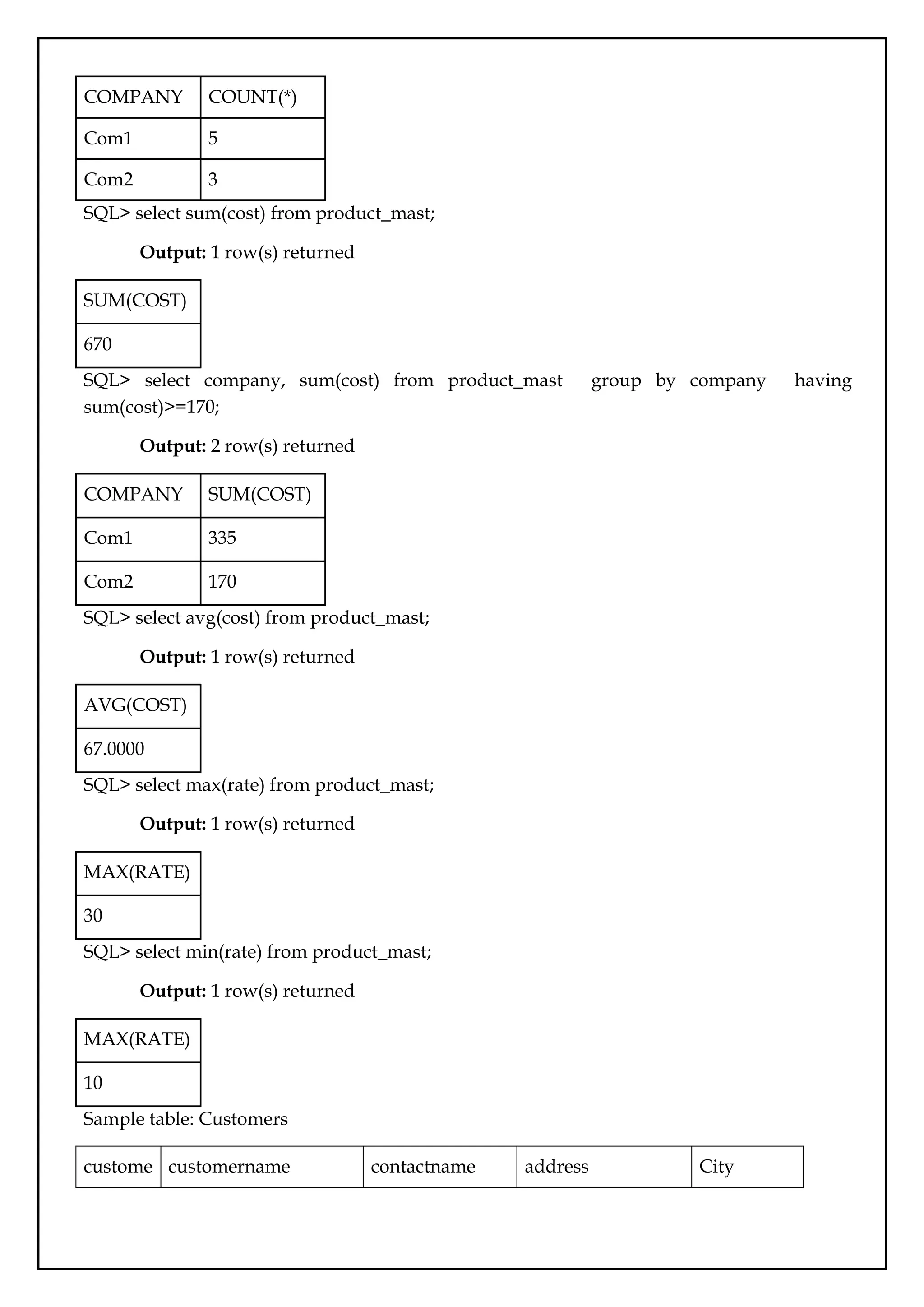
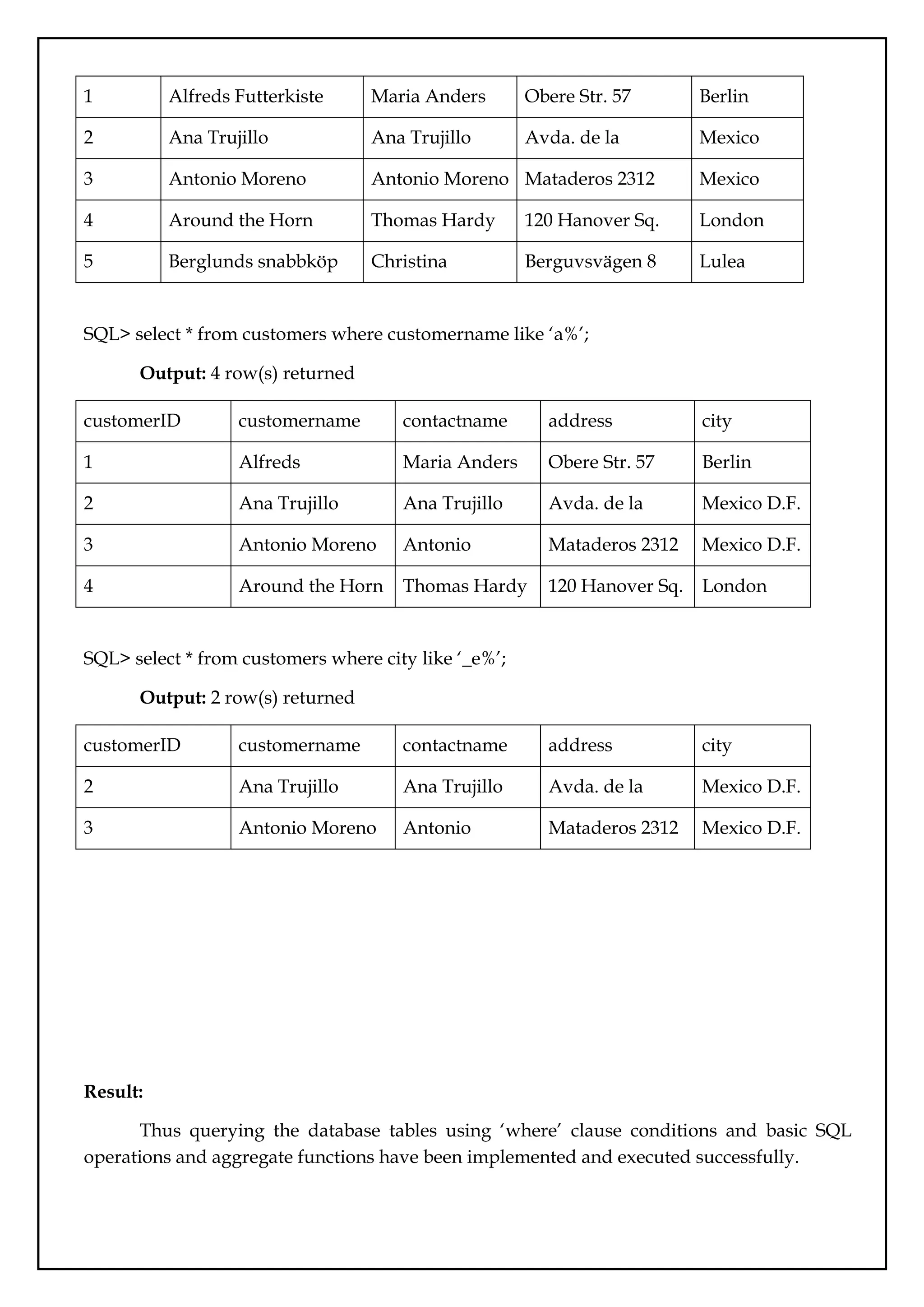
![Ex.No.:04
Sub queries
Date:
Aim:
To query the database tables and explore sub queries.
Description:
A Subquery or Inner query or a Nested query is a query within another SQL query
and embedded within the WHERE clause, HAVING clause, FROM clause.
A subquery is used to return data that will be used in the main query as a condition to
further restrict the data to be retrieved.
Subqueries can be used with the SELECT, INSERT, UPDATE, and DELETE statements
along with the operators like =, <, >, >=, <=, IN, BETWEEN, etc.
Rules that subqueries must follow −
● Subqueries must be enclosed within parentheses.
● A subquery can have only one column in the SELECT clause, unless multiple columns
are in the main query for the subquery to compare its selected columns.
● An ORDER BY command cannot be used in a subquery, although the main query can
use an ORDER BY. The GROUP BY command can be used to perform the same
function as the ORDER BY in a subquery.
● Subqueries that return more than one row can only be used with multiple value
operators such as the IN operator.
● A subquery cannot be immediately enclosed in a set function.
● The BETWEEN operator cannot be used with a subquery. However, the BETWEEN
operator can be used within the subquery.
Subqueries with the SELECT Statement
Subqueries are most frequently used with the SELECT statement.
Syntax : SELECT column_name [, column_name ] FROM table1 [, table2 ] WHERE
column_name OPERATOR (SELECT column_name [, column_name ] FROM table1 [, table2 ]
[WHERE])
Subqueries with the INSERT Statement
Subqueries also can be used with INSERT statements. The INSERT statement uses the
data returned from the subquery to insert into another table. The selected data in the
subquery can be modified with any of the character, date or number functions.
Syntax : INSERT INTO table_name [ (column1 [, column2 ]) ] SELECT [ *|column1 [,
column2 ] FROM table1 [, table2 ] [ WHERE VALUE OPERATOR ]](https://image.slidesharecdn.com/databasemanagementlab-250424094923-0c8b9987/75/CS3481_Database-Management-Laboratory-pdf-27-2048.jpg)
![Subqueries with the UPDATE Statement
The subquery can be used in conjunction with the UPDATE statement. Either single or
multiple columns in a table can be updated when using a subquery with the UPDATE
statement.
Syntax : UPDATE table SET column_name = new_value [WHERE OPERATOR
[VALUE] (SELECT COLUMN_NAME FROM TABLE_NAME) [ WHERE) ]
Subqueries with the DELETE Statement
The subquery can be used in conjunction with the DELETE statement like with any
other statements mentioned above.
Syntax : DELETE FROM TABLE_NAME [ WHERE OPERATOR [ VALUE ] (SELECT
COLUMN_NAME FROM TABLE_NAME) [ WHERE) ]
IN/NOT IN: The IN operator allows to specify multiple values in a WHERE clause.
Syntax: SELECT column_name(s) FROM table_name WHERE column_name
[IN/NOT IN] (value1, value2, ...);
or
SELECT column_name(s) FROM table_name WHERE column_name [IN/NOT IN] (SELECT
STATEMENT);
Queries
Table name: Customer
ID NAME AGE ADDRESS SALARY
1 Ramesh 35 Ahmedabad 2000.00
2 Khilan 25 Delhi 1500.00
3 Kaushik 23 Kota 2000.00
4 Chaitali 25 Mumbai 6500.00
5 Hardik 27 Bopal 8500.00
6 Konal 22 MP 4500.00
7 Muffy 24 Indore 10000.00
SQL> select * from customers where id in (select id from customers where salary > 4500) ;
Output: 3 rows returned](https://image.slidesharecdn.com/databasemanagementlab-250424094923-0c8b9987/75/CS3481_Database-Management-Laboratory-pdf-28-2048.jpg)
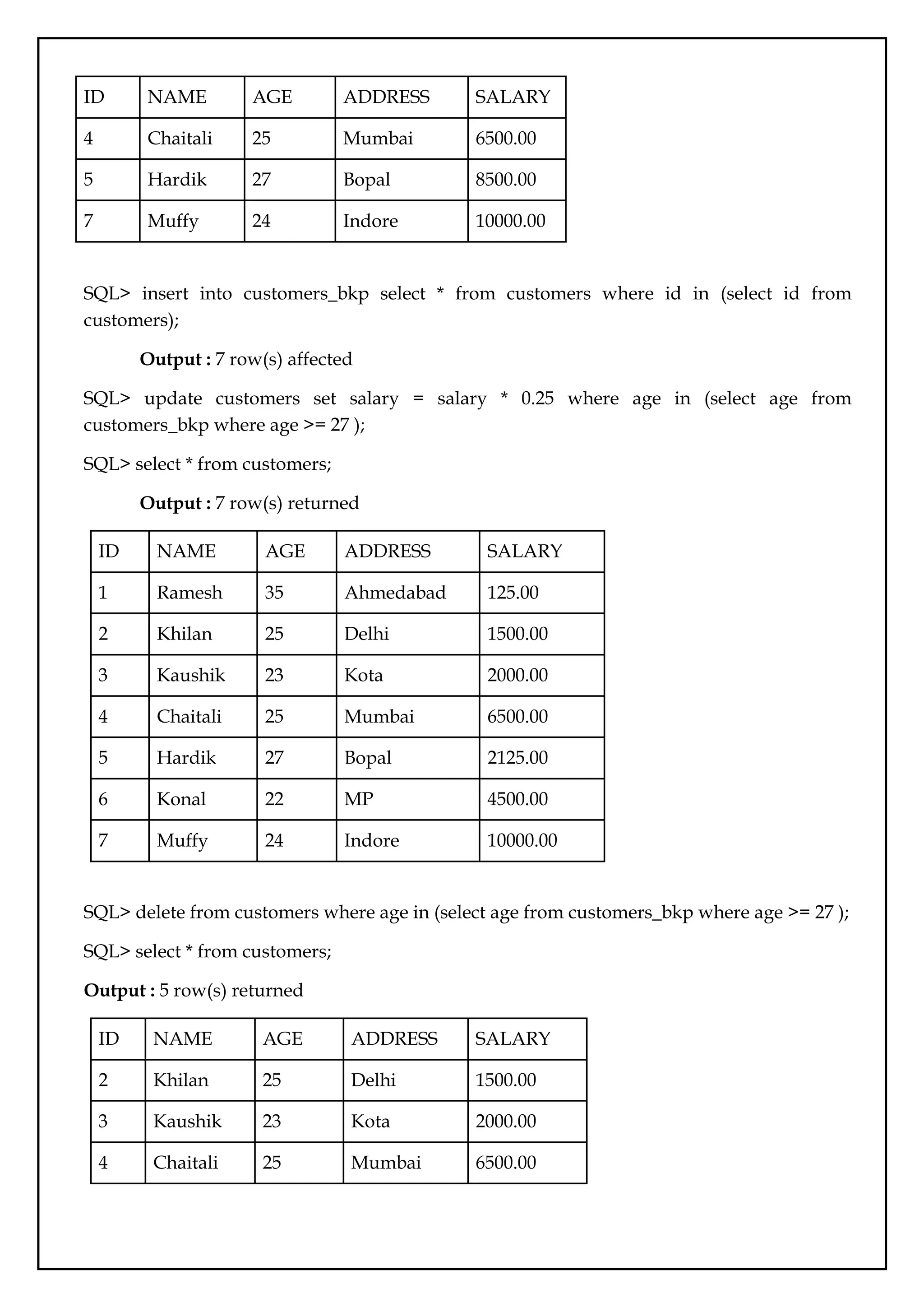
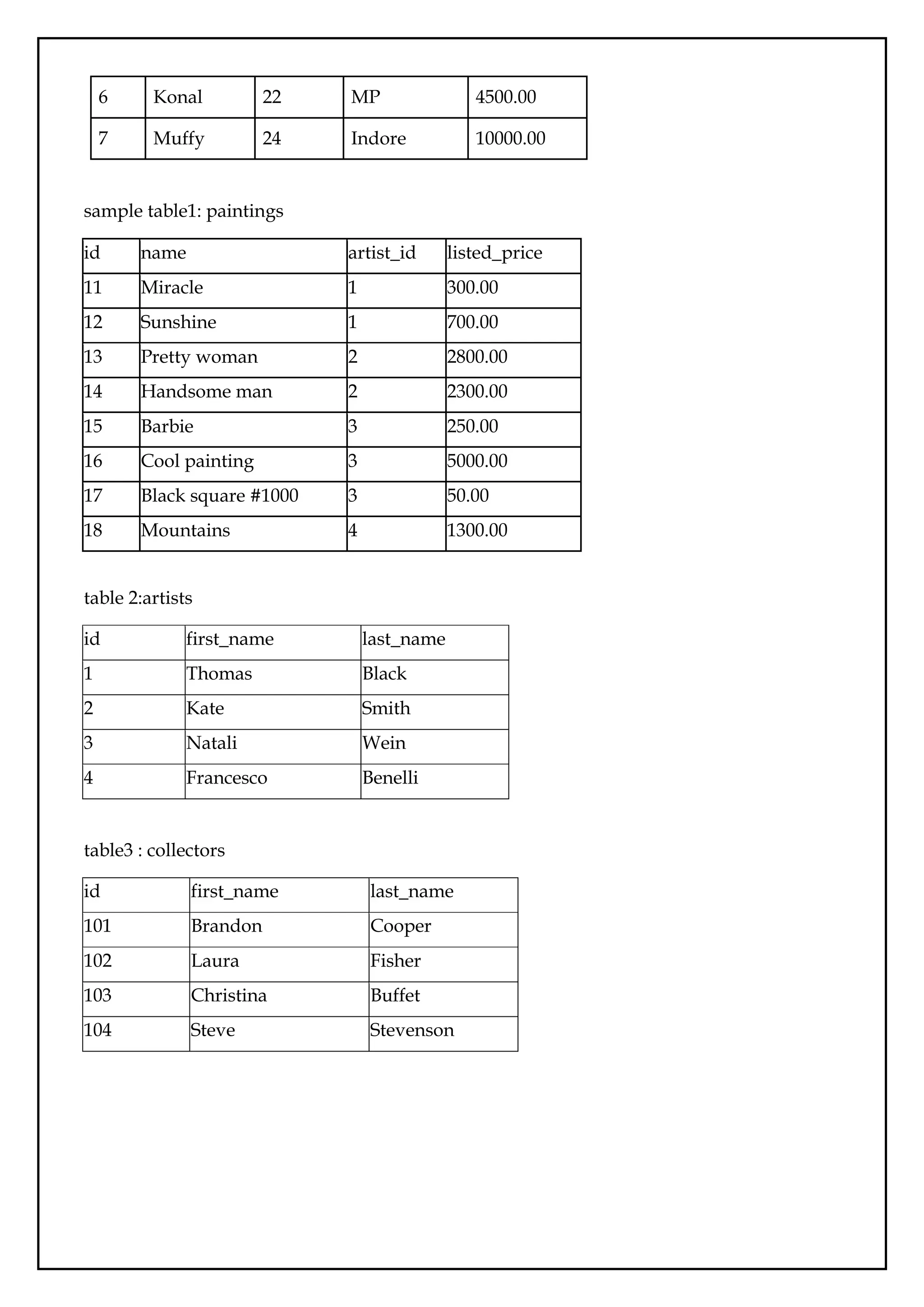
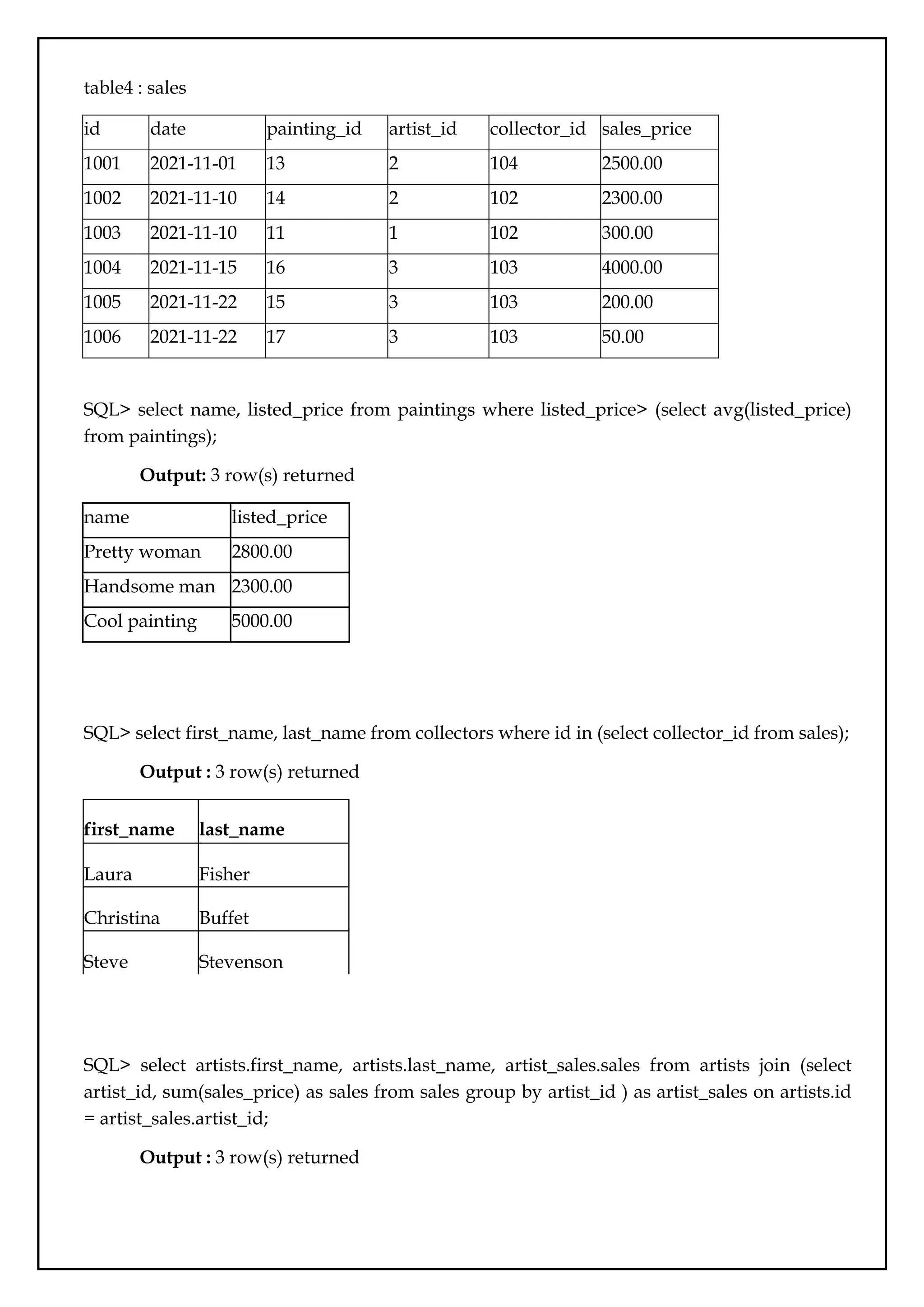
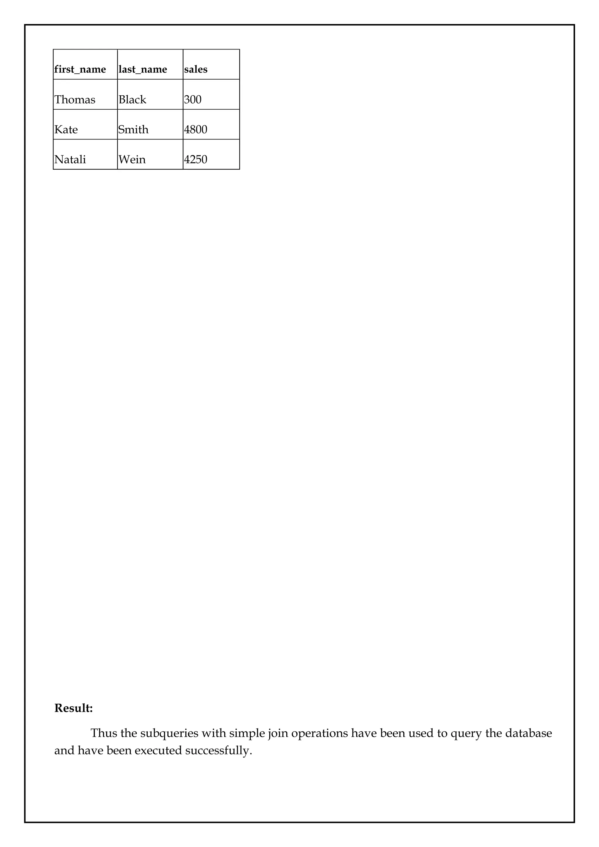
![● RIGHT OUTER JOIN or RIGHT JOIN
● FULL OUTER JOIN
Syntax: Select * FROM table1, table2 WHERE conditions [+];
The SQL LEFT JOIN (specified with the keywords LEFT JOIN and ON) joins two
tables and fetches all matching rows of two tables for which the SQL-expression is true, plus
rows from the first table that do not match any row in the second table.
Syntax : SELECT * FROM table1 LEFT [ OUTER ] JOIN table2 ON
table1.column_name=table2.column_name;
The SQL RIGHT JOIN, joins two tables and fetches rows based on a condition, which
is matching in both the tables ( before and after the JOIN clause mentioned in the syntax
below) , and the unmatched rows will also be available from the table written after the JOIN
clause ( mentioned in the syntax below ).
Syntax: SELECT * FROM table1 RIGHT [ OUTER ] JOIN table2 ON
table1.column_name=table2.column_name;
In SQL the FULL OUTER JOIN combines the results of both left and right outer joins
and returns all (matched or unmatched) rows from the tables on both sides of the join clause.
Syntax : SELECT * FROM table1 FULL OUTER JOIN table2 ON
table1.column_name=table2.column_name;
Queries:
table1-Customers
customer_id first_name
1 John
2 Robert
3 David
4 John
5 Betty
Table2-Orders
order_id amount customer_id
1 200 10
2 500 3](https://image.slidesharecdn.com/databasemanagementlab-250424094923-0c8b9987/75/CS3481_Database-Management-Laboratory-pdf-34-2048.jpg)
![3 300 6
4 800 5
5 150 8
SQL> SELECT Customers.customer_id, Customers.first_name, Orders.amount FROM
Customers JOIN Orders ON Customers.customer_id = Orders.customer_id;
Query with aliases:
SQL> SELECT C.customer_id AS cid, C.first_name AS name, O.amount FROM Customers
AS C JOIN Orders AS O ON C.customer_id = O.customer_id;
Output: 2 row(s) returned
customer_i
d
first_name amount
3 David 500
5 Betty 800
[Note: Above query also represents INNER JOIN, EQUI JOIN(equality operator is used)]
SQL> SELECT * FROM Customers NATURAL JOIN Orders;
Output: 2 row(s) returned
customer_id first_name order_id amount
3 David 2 500
5 Betty 4 800
SQL>SELECT * FROM Customers NATURAL JOIN Orders WHERE orders.amount>500;
Output: 1 row(s) returned
customer_id first_name order_id amount
5 Betty 4 800
SQL> SELECT * FROM Customers LEFT OUTER JOIN Orders ON Customers.customer_id
= Orders.customer_id;
Output: 5 row(s) returned](https://image.slidesharecdn.com/databasemanagementlab-250424094923-0c8b9987/75/CS3481_Database-Management-Laboratory-pdf-35-2048.jpg)
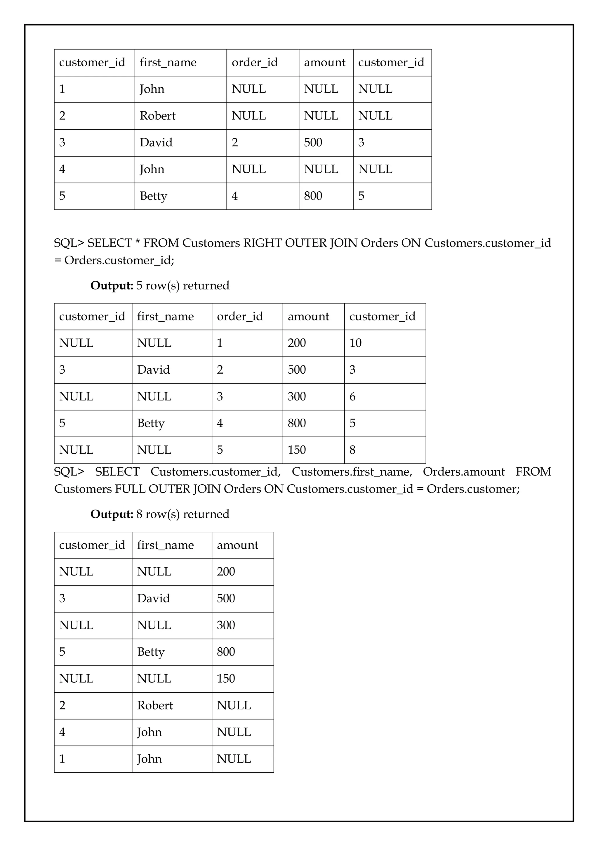

![Ex.No.:06
User Defined Functions and Procedures
Date:
Aim:
To write and execute user defined functions and stored procedures in SQL.
Description:
Stored Procedures:
A Stored Procedure is a precompiled object stored in the database. It makes use of
parameters to pass values and customize results. Parameters are used to specify the columns
in a table in which the query operates and returns results.
Stored procedures can also include the IF, CASE, and LOOP control flow statements
that procedurally implement the code.
Syntax to create Stored Procedure:
DELIMITER $$
CREATE PROCEDURE procedure_name [[IN | OUT | INOUT] parameter_name
datatype [, parameter datatype]) ]
BEGIN
Declaration_section
Executable_section
END $$
DELIMITER ;
Here, the first DELIMITER argument sets the default delimiter to &&, while the last
DELIMITER argument sets it back to the semicolon ;.
The parameter modes are:
IN – Use to pass a parameter as input. When it is defined, the query passes an argument to
the stored procedure. The value of the parameter is always protected.
OUT – Use to pass a parameter as output. You can change the value within the stored
procedure, and the new value is passed back to the calling program.
INOUT – A combination of IN and OUT parameters. The calling program passes the
argument, and the procedure can modify the INOUT parameter, passing the new value back
to the program.
Execute the stored procedure by,](https://image.slidesharecdn.com/databasemanagementlab-250424094923-0c8b9987/75/CS3481_Database-Management-Laboratory-pdf-38-2048.jpg)
![CALL procedure_name;
To alter Stored Procedure
Altering a stored procedure means to change the characteristics of a procedure. There
is no statement in MySQL for modifying the parameters or the body of a stored procedure.
To change parameters or the body, drop the stored procedure and create a new one.
Syntax:
ALTER PROCEDURE procedure_name
COMMENT 'Insert comment here';
To drop Stored Procedure
To drop (delete) a procedure:
Delete a stored procedure from the server by using the DROP PROCEDURE statement.
Syntax: DROP PROCEDURE [IF EXISTS] stored_procedure_name;
User Defined Functions
The function which is defined by the user is called a user-defined function. MySQL
user-defined functions may or may not have parameters that are optional, but it always
returns a single value that is mandatory.
Syntax: DELIMITER $$
CREATE FUNCTION function_name(Parameter_1 Datatype, Parameter_2
Datatype,. . .,Parameter_n Datatype)
RETURNS Return_datatype
[NOT] DETERMINISTIC
BEGIN
Function Body
Return Return_value
END$$
DELIMITER;
First, specify the name of the user-defined function that needs to be created after the
CREATE FUNCTION statement.
Second, list all the input parameters of the user-defined function inside the
parentheses followed by the function name. By default, all the parameters are IN parameters.
Third, specify the data type of the return value in the RETURNS statement, which can
be any valid MySQL data type.](https://image.slidesharecdn.com/databasemanagementlab-250424094923-0c8b9987/75/CS3481_Database-Management-Laboratory-pdf-39-2048.jpg)
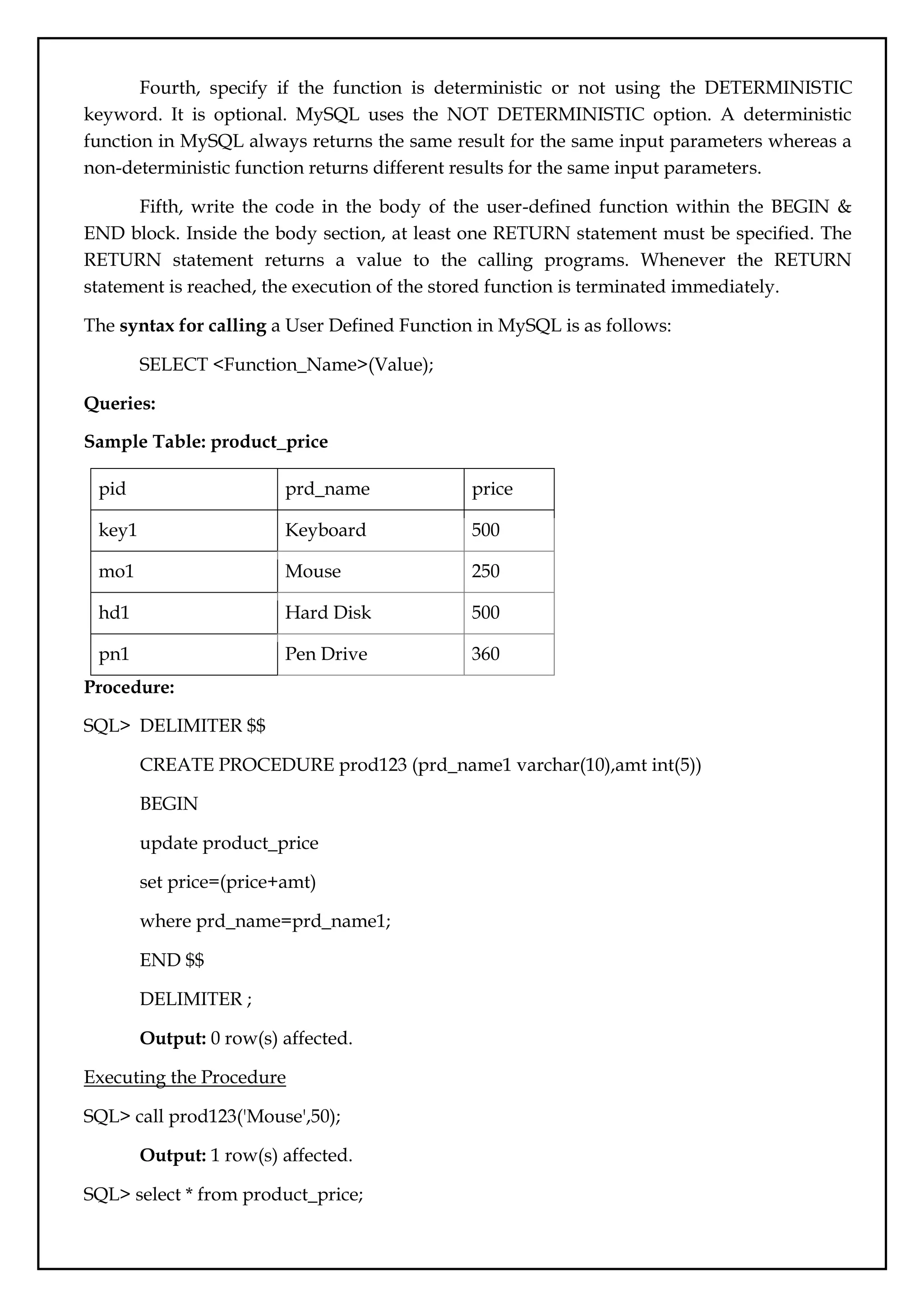
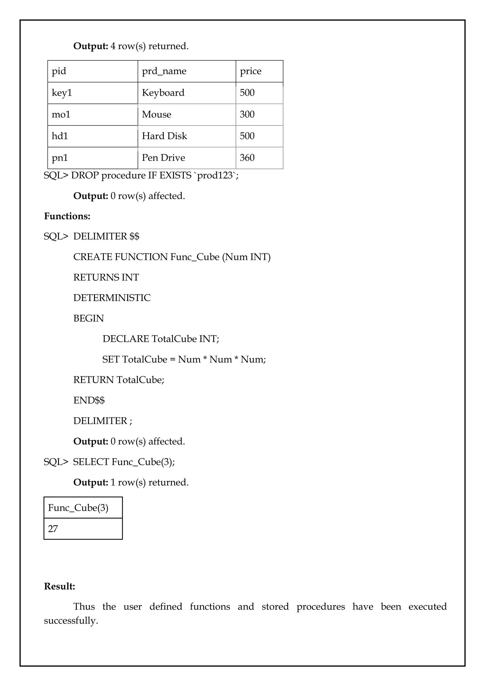

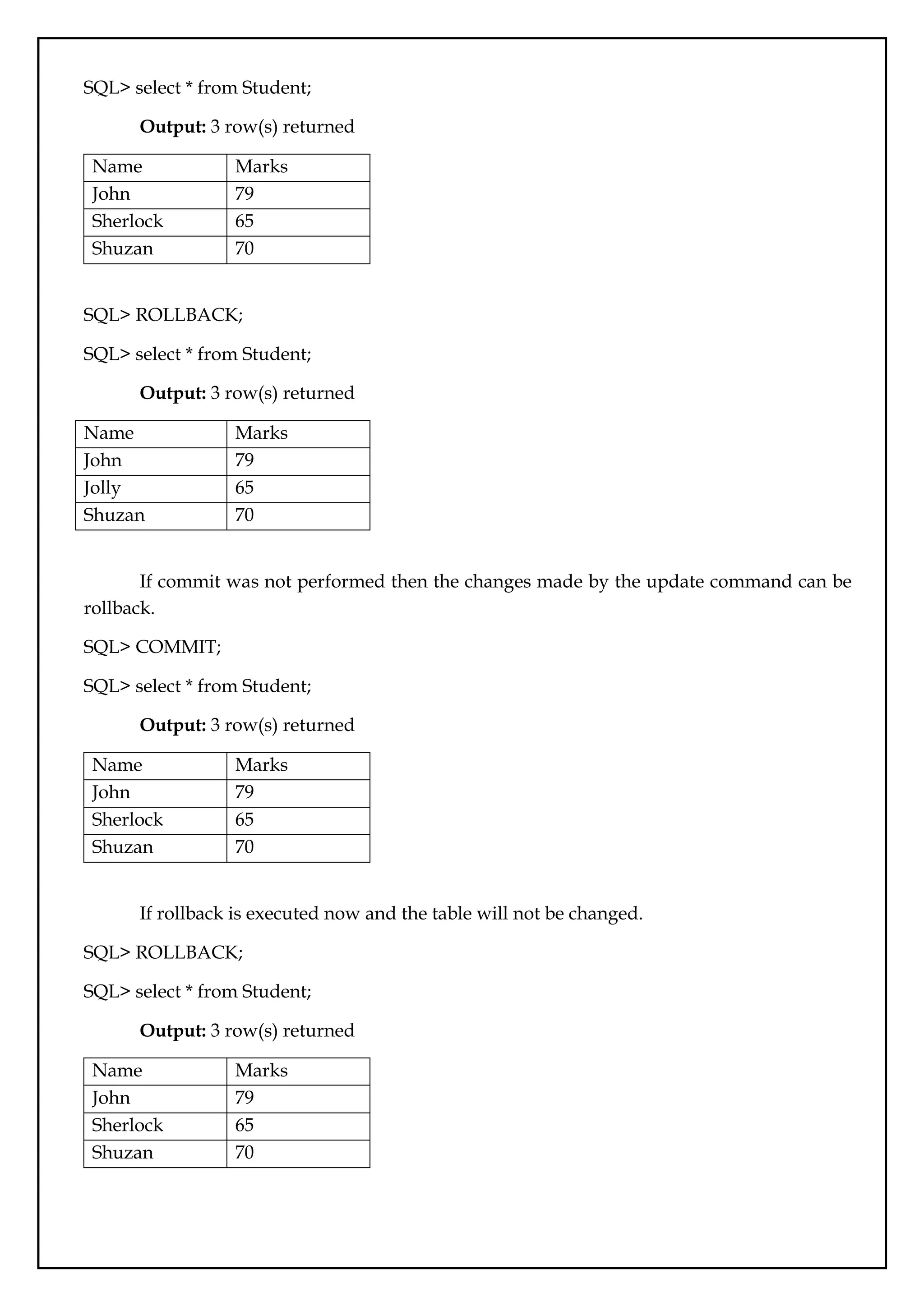
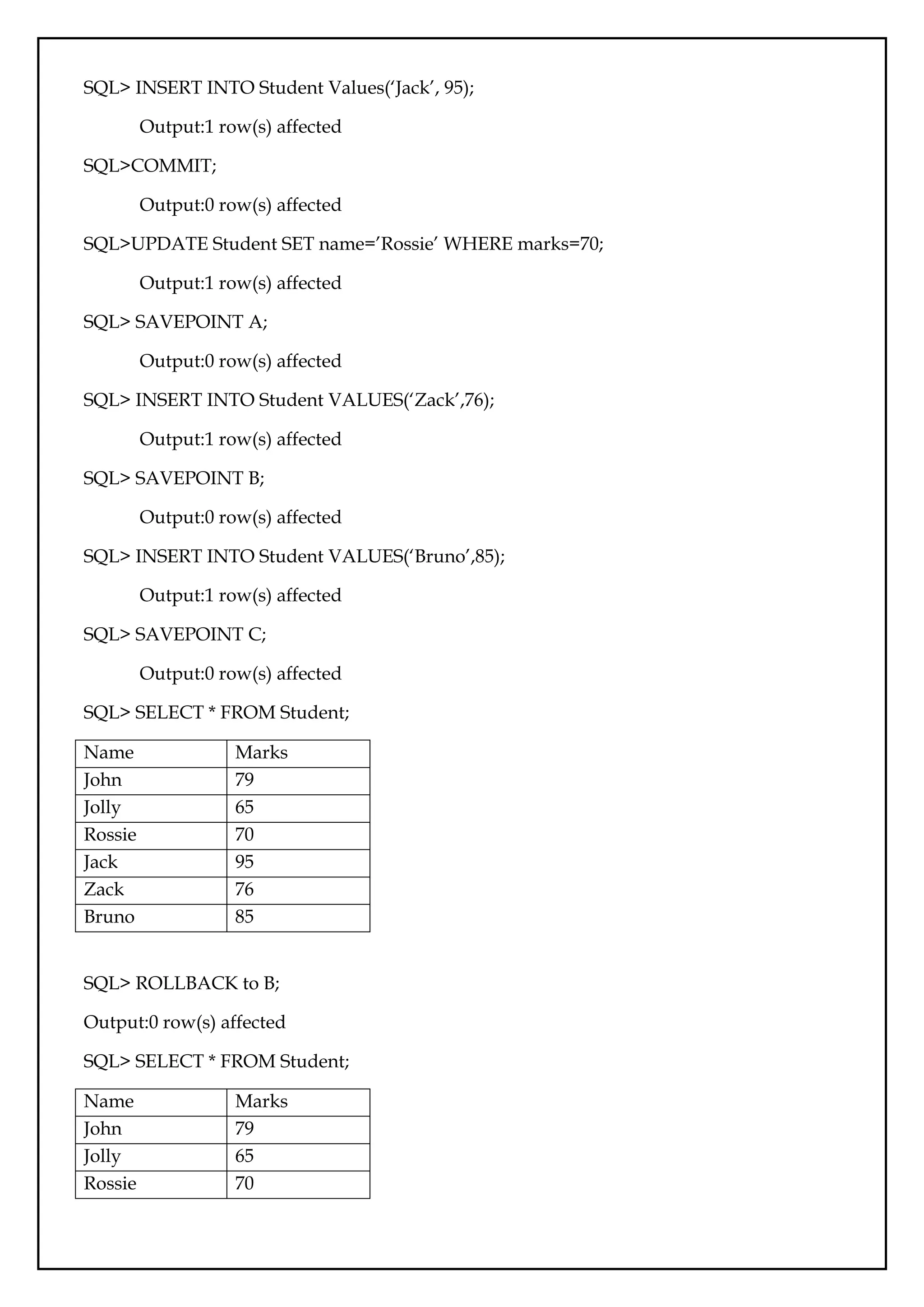
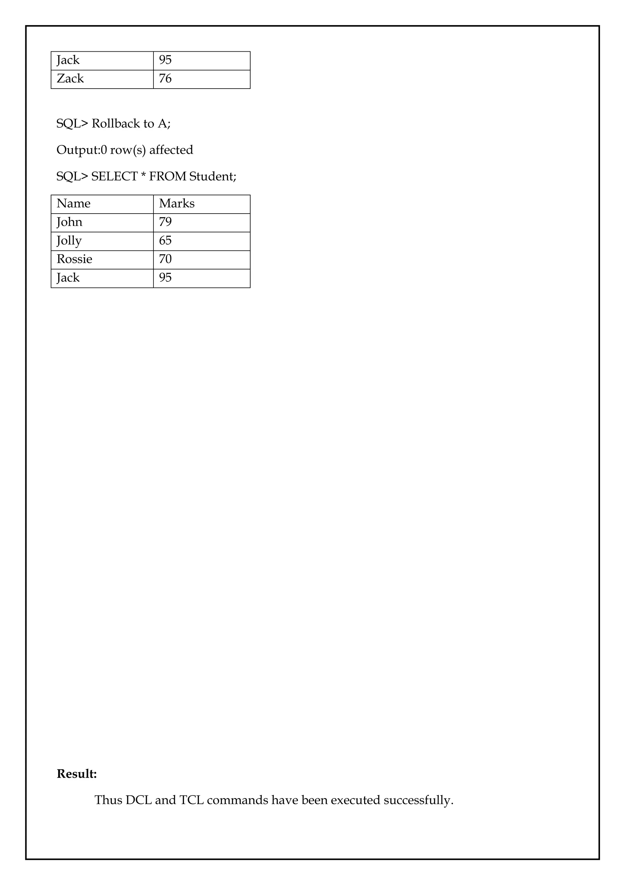
![Ex.No.:08
SQL Triggers
Date:
Aim:
To write SQL Triggers for insert, delete and update operations in the database table.
Description:
A Trigger in Structured Query Language is a set of procedural statements which are
executed automatically when there is any response to certain events on the particular table in
the database. Triggers are used to protect the data integrity in the database.
Syntax:
CREATE TRIGGER Trigger_Name
[ BEFORE | AFTER ] [ Insert | Update | Delete]
ON [Table_Name]
[ FOR EACH ROW | FOR EACH COLUMN ]
AS
Set of SQL Statement
create trigger [trigger_name]: Creates or replaces an existing trigger with the trigger_name.
[before | after]: This specifies when the trigger will be executed.
{insert | update | delete}: This specifies the DML operation.
on [table_name]: This specifies the name of the table associated with the trigger.
[for each row]: This specifies a row-level trigger, i.e., the trigger will be executed for each row
being affected.
[trigger_body]: This provides the operation to be performed as trigger is fired
BEFORE and AFTER of Trigger:
BEFORE triggers run the trigger action before the triggering statement is run. AFTER
triggers run the trigger action after the triggering statement is run.
Queries:
SQL> CREATE TABLE Student_Trigger ( Student_RollNo INT NOT NULL PRIMARY KEY,
Student_FirstName Varchar (100),Student_EnglishMarks INT, Student_PhysicsMarks INT,
Student_ChemistryMarks INT, Student_MathsMarks INT, Student_TotalMarks INT,
Student_Percentage INT);
Output: 0 row(s) affected.](https://image.slidesharecdn.com/databasemanagementlab-250424094923-0c8b9987/75/CS3481_Database-Management-Laboratory-pdf-47-2048.jpg)
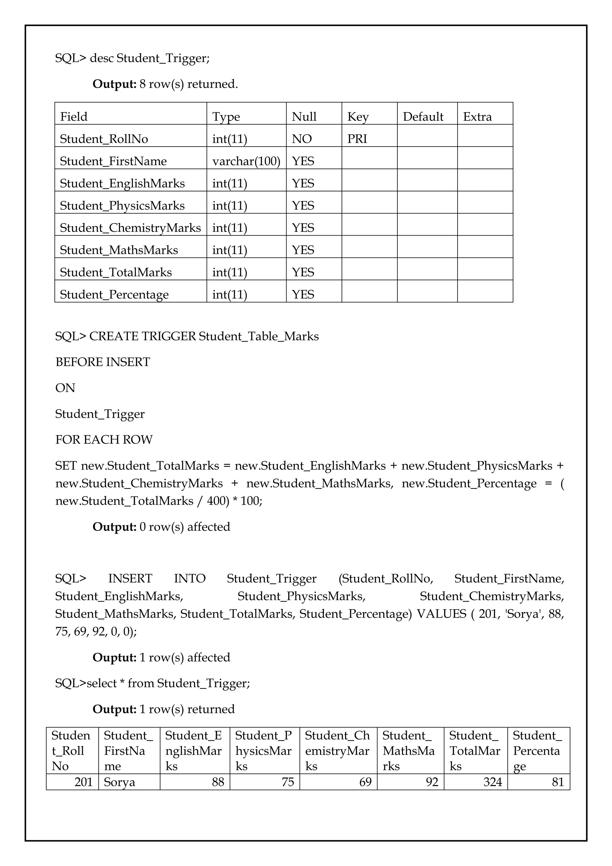

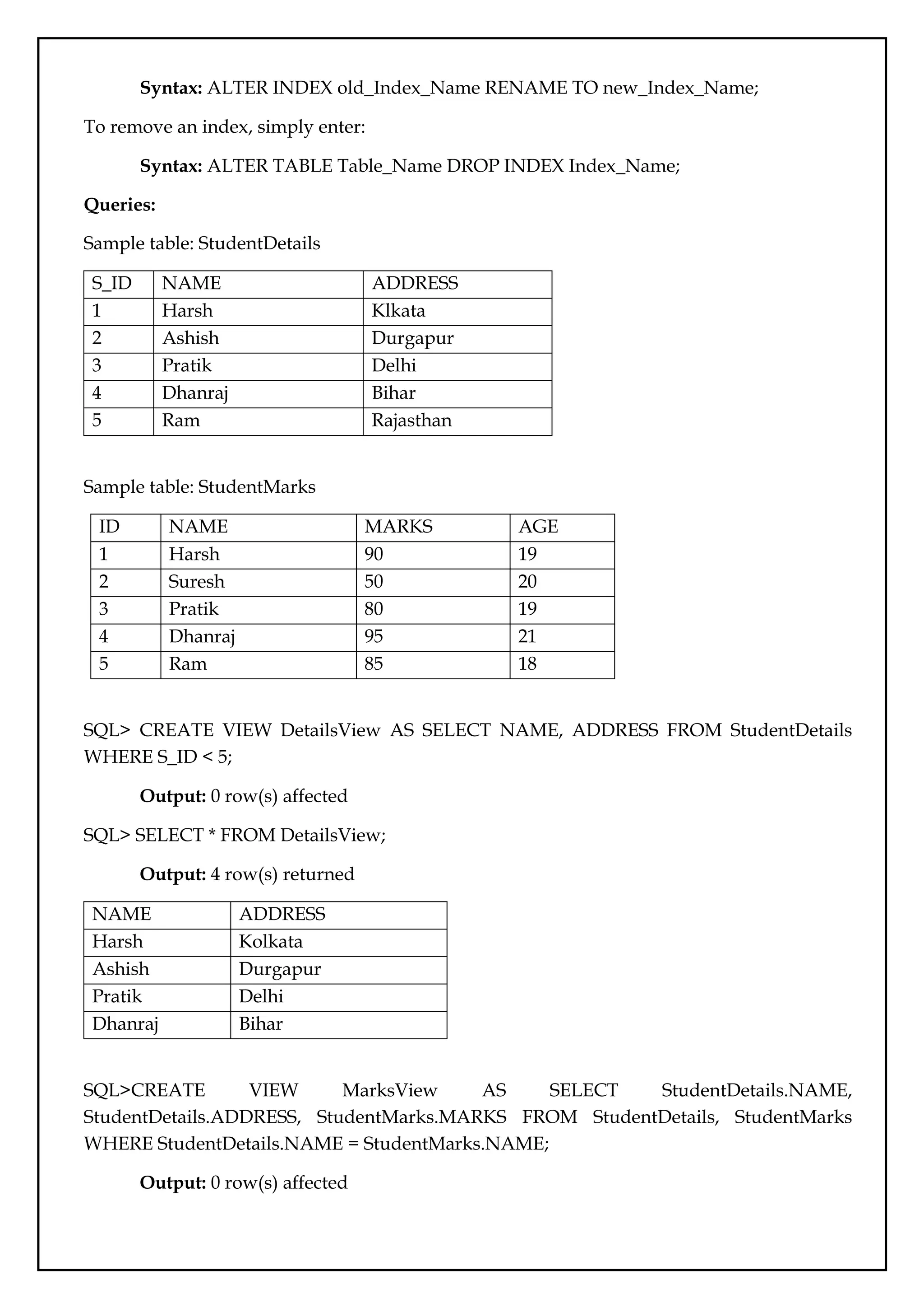
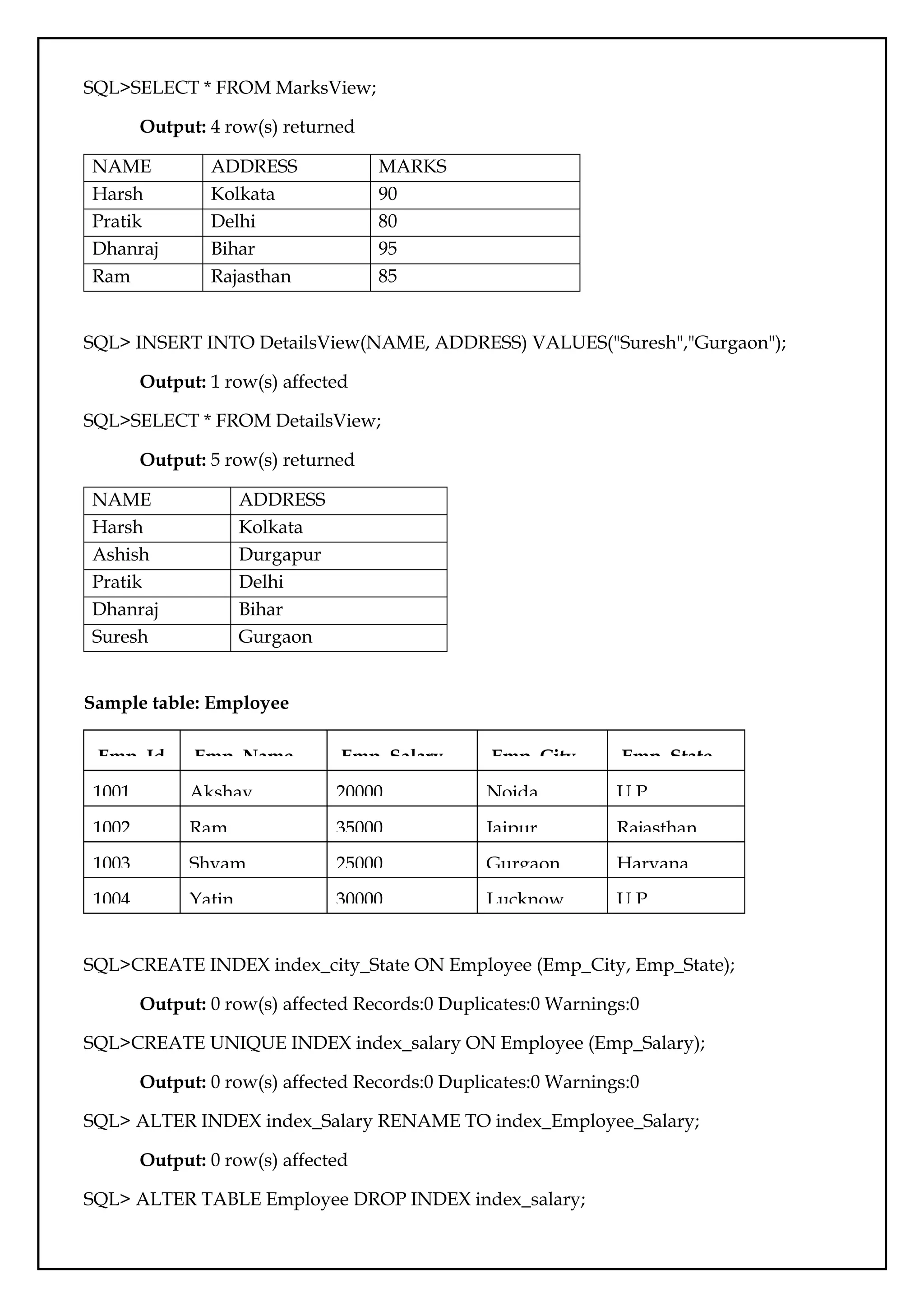

![{
course: "java",
details: {
duration: "6 months",
Trainer: "Sonoo jaiswal"
},
Batch: [ { size: "Small", qty: 15 }, { size: "Medium", qty: 25 } ], category: "Programming
language"
}
)
WriteResult({ "nInserted": 1})
Drop Database:
> db.dropDatabase()
{ "dropped": "javatpointdb", "ok": 1}
Create collection :
>db.SSSIT.insert({"name" : "seomount"})
>show collections
SSSIT
db.collection_name.find()
{ "_id" : ObjectId("56482d3e27e53d2dbc93cef8"), "course" : "java", "details" :
{ "duration" : "6 months", "Trainer" : "Sonoo jaiswal" }, "Batch" :
[ {"size" : "Small", "qty" : 15 }, { "size" : "Medium", "qty" : 25 } ],
"category" : "Programming language" }
Neo4j CQL
Create nodes:
Open the localhost on the browser: http://localhost:7474/browser/ and use the following
code:
CREATE (single);](https://image.slidesharecdn.com/databasemanagementlab-250424094923-0c8b9987/75/CS3481_Database-Management-Laboratory-pdf-60-2048.jpg)