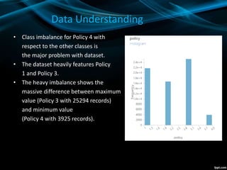
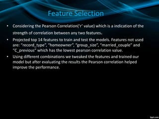
This document summarizes a machine learning project for an insurance company to predict customer purchasing behavior. It discusses: - The objective is to predict the policy number and price a customer will purchase using historical customer data. - The datasets include customer session and purchase histories. There is class imbalance with some policies having much more data than others. - Data preprocessing included removing duplicates, outliers, and normalization. Feature selection used Pearson correlation to identify the most important features. 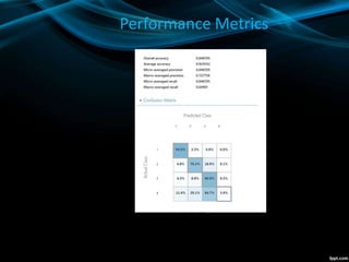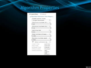- SMOTE oversampling was used to address class imbalance for the policy number classification problem. Two models - decision forest and neural network - were evaluated for classification and regression. 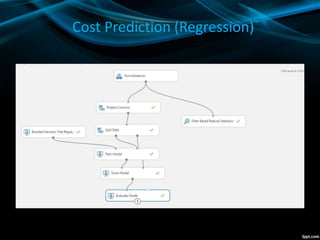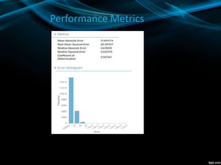- The decision forest model performed best for classification, while boosted decision

1. Competition ‘16
Machine Learning Project

2. Data Mining Stages

3. Objective
• To predict the policy number and the price quoted for that
policy, customer is more likely to purchase.
• The data provided is the historical data from an Insurance
company which provides session history as well as
purchased history of its customers.

4. Datasets
• Train.csv
• Train_Short.csv

5. Data Understanding
• Class imbalance for Policy 4 with
respect to the other classes is
the major problem with dataset.
• The dataset heavily features Policy
1 and Policy 3.
• The heavy imbalance shows the
massive difference between maximum
value (Policy 3 with 25294 records)
and minimum value
(Policy 4 with 3925 records).

6. Approach
• Analyzed the shopping patterns of the customer by looking at Train.csv
dataset.
• Duplicates and outliers(Calculated the standard deviation for each data point
and attribute. Excluded the data points which are out of standard deviation.)
were removed.
• Data was normalized using python.
• Problem statement consists of 2 parts:
– predicting the policy (Classification)
– predicting the cost of the policy (Regression)
• 2 different models were trained and tested using two different algorithms in
Microsoft Azure Machine Learning Suite.

7. Data Preparation
Findings
– Observances like unique customer_id (67,663 in total) has atleast 3 unique
shopping_pt i.e 1,2,3. The pattern is extracted from the Train.csv file.
– Combination of this information aided with the session history of every
customer up to three shopping points and removal of anomalies like
duplication, un uniformity is done.
Data Normalization
– For the high range attributes such as location, data normalization is done
for better results.
– We used normalize_features(feature_set) function in python for
normalization.
Feature Selection
– Considered the Pearson Correlation, the “Filter-Based Feature Selection”
module was employed in Azure to cut down irrelevant features.

8. Feature Selection
• Considering the Pearson Correlation(‘r’ value) which is a indication of the
strength of correlation between any two features.
• Projected top 14 features to train and test the models. Features not used
are: “record_type”, “homeowner”, “group_size”, “married_couple” and
“C_previous” which has the lowest pearson correlation value.
• Using different combinations we tweaked the features and trained our
model but after evaluating the results the Pearson correlation helped
improve the performance.

9. Synthetic Minority Over-Sampling Technique
(SMOTE)
• Smote is a technique employed to over sample the minority class in our
multi-class Classification problem.
• Through this the immense gap in between the values of the four policy
classes in comparison to other classes was reduced.
• Smote is a common data manipulation technique for increasing the number
of cases to create a more balanced dataset.
• Since the instances of policy number 4 is almost seven times less than the
instances of policy 3, we increased the SMOTE sampling to 300% which
increased the accuracy of the classification model by 15%.

10. Policy Prediction(Classification)
Building Model
• Implemented 2 different algorithms on our training set and after
evaluating their performance, Multiclass Decision Forest turned out the
better results among them both.
• The Decision Forest produced better performance and worked better
towards resolving the class imbalance in the data.
• Tune Model Hyperparameter” helped evaluating the performance of our
model for different combinations of parameter values.
• Through this we were able to conclude that our model works best when
the Decision trees are low in number but high in depth.

11. Classification (Multi-Class Decision Forest Model)

12. Parameter Values

13. Performance Metrics

14. Cost Prediction (Regression)
• Model-1
– Used Boosted Decision Tree Regression module to create an ensemble of
regression trees using boosting
– The term Boosting implies that every tree is dependent upon its
preceding tree and learns by fitting the residual of the trees that
preceded it.
• Model-2
– Used Neural Network Regression to create a regression model which is a
customizable neural network algorithm.

15. Cost Prediction (Regression)
Building Model
– The “Root Mean Squared Error” for Neural Network Regression came out
to be 36.85 while for Boosted Decision Tree Regression it was 30 which
clearly shows Boosted Decision Tree Regression is working better for our
dataset.
– With the help of “Tune Model Hyperparameter” , the “Coefficient of
Determination” was achieved close to 0.50 and the “Root Mean Squared
error” close to 23.46(approx.)
– We figured out the best parameters value of Boosted Decision Tree
Regression should have Maximum number of Leaf Nodes to be 20 and
Maximum number of trees to be 20 with learning rate 0.2.

16. Cost Prediction (Regression)

17. Algorithm Properties

18. Performance Metrics

19. THANK YOU