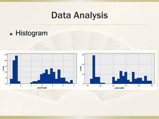
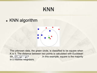
Classification Technique KNN in
           Data Mining
       ---on dataset “Iris”


      Comp722 data mining
        Kaiwen Qi, UNC
          Spring 2012
Outline
   Dataset introduction
   Data processing
   Data analysis
   KNN & Implementation
   Testing
Dataset
   Raw dataset
    Iris(http://archive.ics.uci.edu/ml/datasets/Iris)


                                                                 5 Attributes
                                                (a) Raw
    150 total records                                                     Sepal length in cm
                                                data                     (continious number)
                                                                            Sepal width in cm
                                                                          (continious number)
                  50 records Iris Setosa                                   Petal length in cm
                                                                          (continious number)

                                                                            Petal width in cm
                  50 records Iris Versicolour                             (continious number)
                                                                                   Class
                                                                        (nominal data:
                  50 records Iris Virginica                                  Iris Setosa
                                                                             Iris Versicolour
                                                                             Iris Virginica)

       (b) Data
                                                             (C) Data
       organization
Classification Goal
   Task
Data Processing
   Original data
Data Processing
• Balanced distribution
Data Analysis
   Statistics
Data Analysis
   Histogram
Data Analysis
   Histogram
KNN
   KNN algorithm


    The unknown data, the green circle, is classified to be square when
    K is 5. The distance between two points is calculated with Euclidean
    distance d(p, q)=         . .In this example, square is the majority
    in 5 nearest neighbors.
KNN
   Advantage
       the skimpiness of implementation. It is good
        at dealing with numeric attributes.
       Does not set up the model and just imports
        the dataset with very low computer overhead.
       Does not need to calculate the useful attribute
        subset. Compared with naïve Bayesian, we
        do not need to worry about lack of available
        probability data
Implementation of KNN
   Algorithm
        Algorithm: KNN. Asses a classification label from training data for an
         unlabeled data
         Input: K, the number of neighbors.
         Dataset that include training data
        Output: A string that indicates unknown tuple’s classification

    Method:
     Create a distance array whose size is K
     Initialize the array with the distances between the unlabeled tuple with
      first K records in dataset
     Let i=k+1
     calculate the distance between the unlabeled tuple with the (k+1)th
      record in dataset, if the distance is greater than the biggest distance in
      the array, replace the old max distance with the new distance; i=i+1
     repeat step (4) until i is greater than dataset size(150)
     Count the class number in the array, the class of biggest number is
      mining result
Implementation of KNN
   UML
Testing
   Testing (K=7, total 150 tuples)
Testing
   Testing (K=7, 60% data as training data)
Testing
   Input random distribution dataset


               Random dataset


      Accuracy test:
Performance
   Comparison
     Decision tree
    Advantage                                    Naïve Bayesian
    • comprehensibility
    • construct a decision tree without any     Advantage
      domain knowledge                          • relatively simply.
    • handle high dimensional                   • By simply calculating
    • By eliminating unrelated attributes         attributes frequency from
      and tree pruning, it simplifies             training datanand without
      classification calculation                  any other operations (e.g.
    Disadvantage                                  sort, search),
    • requires good quality of training data.   Disadvantage
    • usually runs in memory                    • The assumption of
    • Not good at handling continuous             independence is not right
      number features.                          • No available probability data
                                                  to calculate probability
Conclusion
   KNN is a simple algorithm with high
    classification accuracy for dataset with
    continuous attributes.
   It shows high performance with balanced
    distribution training data as input.
Thanks
Question?

Data mining project presentation

  • 1.
    Classification Technique KNNin Data Mining ---on dataset “Iris” Comp722 data mining Kaiwen Qi, UNC Spring 2012
  • 2.
    Outline  Dataset introduction  Data processing  Data analysis  KNN & Implementation  Testing
  • 3.
    Dataset  Raw dataset Iris(http://archive.ics.uci.edu/ml/datasets/Iris) 5 Attributes (a) Raw 150 total records Sepal length in cm data (continious number) Sepal width in cm (continious number) 50 records Iris Setosa Petal length in cm (continious number) Petal width in cm 50 records Iris Versicolour (continious number) Class (nominal data: 50 records Iris Virginica Iris Setosa Iris Versicolour Iris Virginica) (b) Data (C) Data organization
  • 4.
  • 5.
    Data Processing  Original data
  • 6.
  • 7.
  • 8.
  • 9.
  • 10.
    KNN  KNN algorithm The unknown data, the green circle, is classified to be square when K is 5. The distance between two points is calculated with Euclidean distance d(p, q)= . .In this example, square is the majority in 5 nearest neighbors.
  • 11.
    KNN  Advantage  the skimpiness of implementation. It is good at dealing with numeric attributes.  Does not set up the model and just imports the dataset with very low computer overhead.  Does not need to calculate the useful attribute subset. Compared with naïve Bayesian, we do not need to worry about lack of available probability data
  • 12.
    Implementation of KNN  Algorithm  Algorithm: KNN. Asses a classification label from training data for an unlabeled data Input: K, the number of neighbors. Dataset that include training data Output: A string that indicates unknown tuple’s classification Method:  Create a distance array whose size is K  Initialize the array with the distances between the unlabeled tuple with first K records in dataset  Let i=k+1  calculate the distance between the unlabeled tuple with the (k+1)th record in dataset, if the distance is greater than the biggest distance in the array, replace the old max distance with the new distance; i=i+1  repeat step (4) until i is greater than dataset size(150)  Count the class number in the array, the class of biggest number is mining result
  • 13.
  • 14.
    Testing  Testing (K=7, total 150 tuples)
  • 15.
    Testing  Testing (K=7, 60% data as training data)
  • 16.
    Testing  Input random distribution dataset Random dataset Accuracy test:
  • 17.
    Performance  Comparison Decision tree Advantage Naïve Bayesian • comprehensibility • construct a decision tree without any Advantage domain knowledge • relatively simply. • handle high dimensional • By simply calculating • By eliminating unrelated attributes attributes frequency from and tree pruning, it simplifies training datanand without classification calculation any other operations (e.g. Disadvantage sort, search), • requires good quality of training data. Disadvantage • usually runs in memory • The assumption of • Not good at handling continuous independence is not right number features. • No available probability data to calculate probability
  • 18.
    Conclusion  KNN is a simple algorithm with high classification accuracy for dataset with continuous attributes.  It shows high performance with balanced distribution training data as input.
  • 19.