This document provides an overview of simultaneous equation models. Some key points:
- Simultaneous equation models account for relationships where one variable is determined by others, which are also determined by the first variable (two-way relationship).
- They consist of multiple equations, with one for each endogenous (jointly determined) variable. The parameters cannot be estimated by looking at single equations.
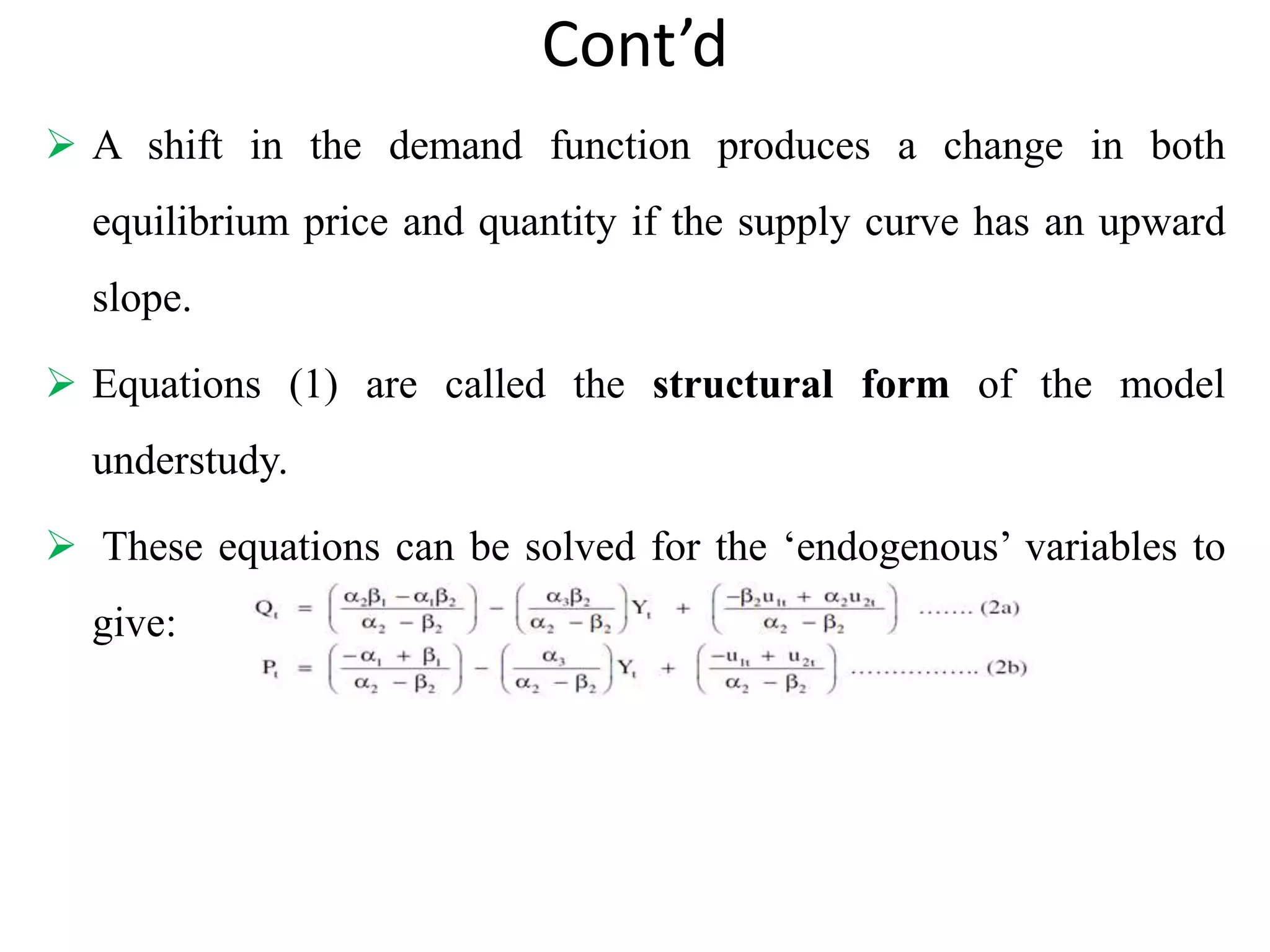
- Reduced form equations express the endogenous variables solely in terms of exogenous variables and error terms. This allows consistent estimation of coefficients using OLS.
- Identification concerns whether the structural form parameters can be uniquely determined from the reduced form parameters. Exact, over- or under-identification can occur.


![The_citric_acid_cycle[1].pdf](https://cdn.slidesharecdn.com/ss_thumbnails/thecitricacidcycle1-230516202238-10c74d1d-thumbnail.jpg?width=640&height=640&fit=bounds)


