Calculus In 3d Geometry Vectors And Multivariate Calculus Draft Nitecki
Calculus In 3d Geometry Vectors And Multivariate Calculus Draft Nitecki
Calculus In 3d Geometry Vectors And Multivariate Calculus Draft Nitecki
Calculus In 3d Geometry Vectors And Multivariate Calculus Draft Nitecki
Calculus In 3d Geometry Vectors And Multivariate Calculus Draft Nitecki
1.
Calculus In 3dGeometry Vectors And Multivariate
Calculus Draft Nitecki download
https://ebookbell.com/product/calculus-in-3d-geometry-vectors-
and-multivariate-calculus-draft-nitecki-9970788
Explore and download more ebooks at ebookbell.com
2.
Here are somerecommended products that we believe you will be
interested in. You can click the link to download.
Calculus In 3d Geometry Vectors And Multivariate Calculus 1st Edition
Zbigniew Nitecki
https://ebookbell.com/product/calculus-in-3d-geometry-vectors-and-
multivariate-calculus-1st-edition-zbigniew-nitecki-10443716
Calculus In 5 Hours Concepts Revealed So You Dont Have To Sit Through
A Semester Of Lectures Dennis Jarecke
https://ebookbell.com/product/calculus-in-5-hours-concepts-revealed-
so-you-dont-have-to-sit-through-a-semester-of-lectures-dennis-
jarecke-46394070
Fractional Calculus In Analysis Dynamics And Optimal Control Jacky
Cresson
https://ebookbell.com/product/fractional-calculus-in-analysis-
dynamics-and-optimal-control-jacky-cresson-51188652
Differential Calculus In Several Variables 1st Edition Marius Ghergu
https://ebookbell.com/product/differential-calculus-in-several-
variables-1st-edition-marius-ghergu-54722852
3.
Barycentric Calculus InEuclidean And Hyperbolic Geometry Ungar Aa
https://ebookbell.com/product/barycentric-calculus-in-euclidean-and-
hyperbolic-geometry-ungar-aa-2048314
Fractional Calculus In Bioengineering Richard L Magin
https://ebookbell.com/product/fractional-calculus-in-bioengineering-
richard-l-magin-28370718
Malliavin Calculus In Finance Theory And Practice 1st Edition Elisa
Alos
https://ebookbell.com/product/malliavin-calculus-in-finance-theory-
and-practice-1st-edition-elisa-alos-29905916
Thomas Calculus In Si Units 14th Edition Hass Joel R Heil Christopher
E
https://ebookbell.com/product/thomas-calculus-in-si-units-14th-
edition-hass-joel-r-heil-christopher-e-34906066
Fractional Calculus In Analysis Dynamics And Optimal Control Jacky
Cresson
https://ebookbell.com/product/fractional-calculus-in-analysis-
dynamics-and-optimal-control-jacky-cresson-5209042
5.
Calculus in 3D
Geometry,Vectors, and
Multivariate Calculus
Zbigniew H. Nitecki
Tufts University
August 19, 2012
6.
ii
This work issubject to copyright. It may be copied for non-commercial
purposes.
7.
Preface
The present volumeis a sequel to my earlier book, Calculus Deconstructed:
A Second Course in First-Year Calculus, published by the Mathematical
Association in 2009. I have used versions of this pair of books for severel
years in the Honors Calculus course at Tufts, a two-semester “boot camp”
intended for mathematically inclined freshmen who have been exposed to
calculus in high school. The first semester of this course, using the earlier
book, covers single-variable calculus, while the second semester, using the
present text, covers multivariate calculus. However, the present book is
designed to be able to stand alone as a text in multivariate calculus.
The treatment here continues the basic stance of its predecessor,
combining hands-on drill in techniques of calculation with rigorous
mathematical arguments. However, there are some differences in emphasis.
On one hand, the present text assumes a higher level of mathematical
sophistication on the part of the reader: there is no explicit guidance in
the rhetorical practices of mathematicians, and the theorem-proof format
is followed a little more brusquely than before. On the other hand, the
material being developed here is unfamiliar territory, for the intended
audience, to a far greater degree than in the previous text, so more effort is
expended on motivating various approaches and procedures. Where
possible, I have followed my own predilection for geometric arguments over
formal ones, although the two perspectives are naturally intertwined. At
times, this may feel like an analysis text, but I have studiously avoided the
temptation to give the general, n-dimensional versions of arguments and
results that would seem natural to a mature mathematician: the book is,
after all, aimed at the mathematical novice, and I have taken seriously the
limitation implied by the “3D” in my title. This has the advantage,
however, that many ideas can be motivated by natural geometric
arguments. I hope that this approach lays a good intuitive foundation for
further generalization that the reader will see in later courses.
Perhaps the fundamental subtext of my treatment is the way that the
theory developed for functions of one variable interacts with geometry to
iii
8.
iv
handle higher-dimension situations.The progression here, after an initial
chapter developing the tools of vector algebra in the plane and in space
(including dot products and cross products), is to first view vector-valued
functions of a single real variable in terms of parametrized curves—here,
much of the theory translates very simply in a coordinate-wise way—then
to consider real-valued functions of several variables both as functions with
a vector input and in terms of surfaces in space (and level curves in the
plane), and finally to vector fields as vector-valued functions of vector
variables. This progression is not followed perfectly, as Chapter 4 intrudes
between Chapter 3, the differential and Chapter 5, the integral calculus of
real-valued functions of several variables, to establish the
change-of-variables formula for multiple integrals.
Idiosyncracies
There are a number of ways, some apparent, some perhaps more subtle, in
which this treatment differs from the standard ones:
Parametrization: I have stressed the parametric representation of curves
and surfaces far more, and beginning somewhat earlier, than many
multivariate texts. This approach is essential for applying calculus to
geometric objects, and it is also a beautiful and satisfying interplay
between the geometric and analytic points of view. While Chapter 2
begins with a treatment of the conic sections from a classical point of
view, this is followed by a catalogue of parametrizations of these
curves, and in § 2.4 a consideration of what should constitute a curve
in general. This leads naturally to the formulation of path integrals
in § 2.5. Similarly, quadric surfaces are introduced in § 3.4 as level
sets of quadratic polynomials in three variables, and the
(three-dimensional) Implicit Function Theorem is introduced to show
that any such surface is locally the graph of a function of two
variables. The notion of parametrization of a surface is then
introduced and exploited in § 3.6 to obtain the tangent planes of
surfaces. When we get to surface integrals in § 5.4, this gives a
natural way to define and calculate surface area and surface integrals
of functions. This approach comes to full fruition in Chapter 6 in the
formulation of the integral theorems of vector calculus.
Determinants and Cross-Products: There seem to be two prevalent
approaches in the literature to introducing determinants: one is
9.
v
formal, dogmatic andbrief, simply giving a recipe for calculation and
proceeding from there with little motivation for it; the other is even
more formal but elaborate, usually involving the theory of
permutations. I believe I have come up with an approach to
introducing 2 × 2 and 3 × 3 determinants (along with crossproducts)
which is both motivated and rigorous, in § 1.6. Starting with the
problem of calculating the area of a planar triangle from the
coordinates of its vertices, we deduce a formula which is naturally
written as the absolute value of a 2 × 2 determinant; investigation of
the determinant itself leads to the notion of signed (i.e., oriented)
area (which has its own charm, and prophesies the introduction of
2-forms in Chapter 6). Going to the analogous problem in space, we
introduce the notion of an oriented area, represented by a vector
(which we ultimately take as the definition of the cross-product, an
approach taken for example by David Bressoud). We note that
oriented areas project nicely, and from the projections of an oriented
area vector onto the coordinate planes come up with the formula for
a cross-product as the expansion by minors along the first row of a
3 × 3 determinant. In the present treatment, various algebraic
properties of determinants are developed as needed, and the relation
to linear independence is argued geometrically.
I have found in my classes that the majority of students have already
encountered (3 × 3) matrices and determinants in high school. I have
therefore put some of the basic material about determinants in a
separate appendix (Appendix E).
“Baby” Linear Algebra: I have tried to interweave into my narrative
some of the basic ideas of linear algebra. As with determinants, I
have found that the majority of my students (but not all) have
already encountered vectors and matrices in their high school
courses, so the basic material on matrix algebra and row reduction is
covered quickly in the text but in more leisurely fashion in
Appendix D. Linear independence and spanning for vectors in
3-space are introduced from a primarily geometric point of view, and
the matrix representative of a linear function (resp. mapping) is
introduced in § 3.2 (resp. § 4.1). The most sophisticated topics from
linear algebra are eigenvectors and eigenfunctions, introduced in
connection with the (optional) Principal Axis Theorem in § 3.10.
The 2 × 2 case is treated separately in § 3.7, without the use of these
tools, and the more complicated 3 × 3 case can be treated as
10.
vi
optional. I havechosen to include this theorem, however, both
because it leads to a nice understanding of quadratic forms (useful in
understanding the second derivative test for critical points) and
because its proof is a wonderful illustration of the synergy between
calculus (Lagrange multipliers) and algebra.
Implicit and Inverse Function Theorems: I believe these theorems
are among the most neglected major results in multivariate calculus.
They take some time to absorb, and so I think it a good idea to
introduce them at various stages in a student’s mathematical
education. In this treatment, I prove the Implicit Function Theorem
for real-valued functions of two and three variables in § 3.4, and then
formulate the Implicit Mapping Theorem for mappings R3 → R2, as
well as the Inverse Mapping Theorem for mappings R2 → R2 and
R3 → R3 in § 4.4. I use the geometric argument attributed to
Goursat by [34] rather than the more sophisticated one using the
contraction mapping theorem. Again, this is a more “hands on”
approach than the latter.
Vector Fields vs. Differential Forms: A number of relatively recent
treatments of vector calculus have been based exclusively on the
theory of differential forms, rather than the traditional formulation
using vector fields. I have tried this approach in the past, but in my
experience it confuses the students at this level, so that they end up
dealing with the theory on a blindly formal basis. By contrast, I find
it easier to motivate the operators and results of vector calculus by
treating a vector field as the velocity of a moving fluid, and so have
used this as my primary approach. However, the formalism of
differential forms is very slick as a calculational device, and so I have
also introduced it interwoven with the vector field approach. The
main strength of the differential forms approach, of course, is that it
generalizes to dimensions higher than 3; while I hint at this, it is one
place where my self-imposed limitation to “3D” is evident.
Format
In general, I have continued the format of my previous book in this one.
As before, exercises come in four flavors:
Practice Problems serve as drill in calculation.
11.
vii
Theory Problems involvemore ideas, either filling in gaps in the
argument in the text or extending arguments to other cases. Some of
these are a bit more sophisticated, giving details of results that are
not sufficiently central to the exposition to deserve explicit proof in
the text.
Challenge Problems require more insight or persistence than the
standard theory problems. In my class, they are entirely optional,
extra-credit assignments.
Historical Notes explore arguments from original sources. There are
many fewer of these than in the previous volume, in large part
because the history of multivariate calculus is not nearly as well
documented and studied as is the history of single-variable calculus.
I have deferred a number of involved, technical proofs to appendices,
especially from § 2.1 (to Appendix A-Appendix C), § 4.3-§ 4.4 (to
Appendix F) and § 5.3 (to Appendix G). As a result, there are more
appendices in this volume than in the previous one. To summarize their
contents:
Appendix A and Appendix B give the details of the classical
arguments in Apollonius’ treatment of conic sections and Pappus’
proof of the focus-directrix property of conics. The results
themselves are presented in § 2.1 of the text.
Appendix C carries out in detail the formulation of the equations of
conic sections from the focus-directrix property, sketched in § 2.1.
Appendix D gives a treatment of matrix algebra, row reduction, and
rank of matrices that is more leisurely and motivated than that in
the text.
Appendix E explains why 2 × 2 and 3 × 3 determinants can be
calculated via expansion by minors along any row or column, that
each is a multilinear function of its rows, and the relation between
determinants and singularity of matrices.
Appendix F Gives details of the proofs of the Inverse Mapping Theorem
in dimensions 2 or more, as well as of the Implicit Function Theorem
for dimensions above 2.
12.
viii
Appendix G carriesout the geometric argument that a coordinate
transformation “stretches” areas (or volumes) by a factor given by
integrating the Jacobian.
Appendix H presents H. Schwartz’s example showing that the definition
of arclength as the supremum of lengths of piecewise linear
approximations cannot be generalized to surface area. This helps
justify the resort to differential formalism in defining surface area in
§ 5.4.
Acknowledgements
As with the previous book, I want to thank Jason Richards who as my
grader in this course over several years contributed many corrections and
useful comments about the text. After he graduated, Erin van Erp acted
as my grader, making further helpful comments. I also affectionately thank
my students over the past few years, particularly Matt Ryan, who noted a
large number of typos and minor errors in the “beta” version of this book.
I have also benefited greatly from much help with TeX packages especially
from the e-forum on pstricks and pst-3D solids run by Herbert Voss, as
well as the “Tex on Mac OS X” elist. My colleague Loring Tu helped me
better understand the role of orientation in the integration of differential
forms. On the history side, Sandro Capparini helped introduce me to the
early history of vectors, and Lenore Feigenbaum and especially Michael N.
Fried helped me with some vexing questions concerning Apollonius’
classification of the conic sections. Scott Maclachlan helped me think
through several somewhat esoteric but useful results in vector calculus. As
always, what is presented here is my own interpretation of their comments,
and is entirely my personal responsibility.
1
Coordinates and Vectors
1.1Locating Points in Space
Rectangular Coordinates
The geometry of the number line R is quite straightforward: the location
of a real number x relative to other numbers is determined—and
specified—by the inequalities between it and other numbers x′: if x < x′
then x is to the left of x′, and if x > x′ then x is to the right of x′.
Furthermore, the distance between x and x′ is just the difference
△x = x′ − x (resp. x − x′) in the first (resp. second) case, a situation
summarized as the absolute value
|△x| = x − x′
.
When it comes to points in the plane, more subtle considerations are
needed. The most familiar system for locating points in the plane is a
rectangular or Cartesian coordinate system. We pick a distinguished
point called the origin and denoted O .
Now we draw two axes through the origin: the first is called the x-axis
and is by convention horizontal, while the second, or y-axis, is vertical.
We regard each axis as a copy of the real line, with the origin
corresponding to zero. Now, given a point P in the plane, we draw a
rectangle with O and P as opposite vertices, and the two edges emanating
1
18.
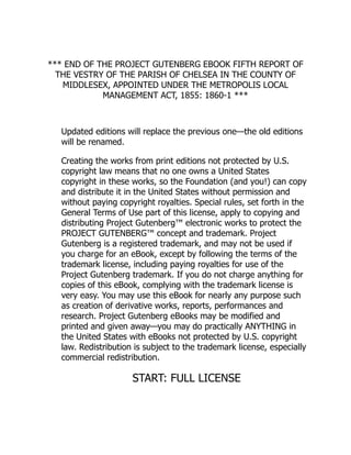
2 CHAPTER 1.COORDINATES AND VECTORS
P
O
y
x
Figure 1.1: Rectangular Coordinates
from O lying along our axes (see Figure 1.1): thus, one of the vertices
between O and P is a point on the x-axis, corresponding to a number x
called the abcissa of P; the other lies on the y-axis, and corresponds to
the ordinate y of P. We then say that the (rectangular or Cartesian)
coordinates of P are the two numbers (x, y). Note that the ordinate
(resp. abcissa) of a point on the x-axis (resp. y-axis) is zero, so the point
on the x-axis (resp. y-axis) corresponding to the number x ∈ R (resp.
y ∈ R) has coordinates (x, 0) (resp. (0, y)).
The correspondence between points of the plane and pairs of real numbers,
as their coordinates, is one-to-one (distinct points correspond to distinct
pairs of numbers, and vice-versa), and onto (every point P in the plane
corresponds to some pair of numbers (x, y), and conversely every pair of
numbers (x, y) represents the coordinates of some point P in the plane). It
will prove convenient to ignore the distinction between pairs of numbers
and points in the plane: we adopt the notation R2 for the collection of all
pairs of real numbers, and we identify R2 with the collection of all points
in the plane. We shall refer to “the point P(x, y)” when we mean “the
point P in the plane whose (rectangular) coordinates are (x, y)”.
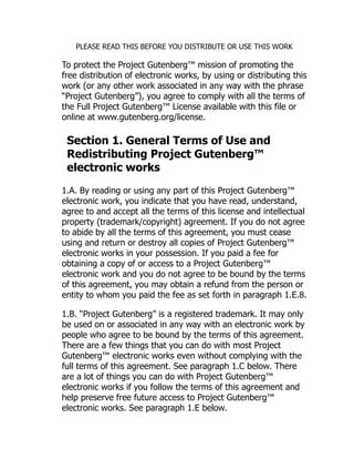
The preceding description of our coordinate system did not specify which
direction along each of the axes is regarded as positive (or increasing). We
adopt the convention that (using geographic terminology) the x-axis goes
“west-to-east”, with “eastward” the increasing direction, and the y-axis
goes “south-to-north”, with “northward” increasing. Thus, points to the
“west” of the origin (and of the y-axis) have negative abcissas, and points
“south” of the origin (and of the x-axis) have negative ordinates
(Figure 1.2).
The idea of using a pair of numbers in this way to locate a point in the
plane was pioneered in the early seventeenth cenury by Pierre de Fermat
19.
1.1. LOCATING POINTSIN SPACE 3
(−, +)
(−, −)
(+, +)
(+, −)
Figure 1.2: Direction Conventions
(1601-1665) and René Descartes (1596-1650). By means of such a scheme,
a plane curve can be identified with the locus of points whose coordinates
satisfy some equation; the study of curves by analysis of the corresponding
equations, called analytic geometry, was initiated in the research of
these two men. Actually, it is a bit of an anachronism to refer to
rectangular coordinates as “Cartesian”, since both Fermat and Descartes
often used oblique coordinates, in which the axes make an angle other
than a right one.1 Furthermore, Descartes in particular didn’t really
consider the meaning of negative values for the abcissa or ordinate.
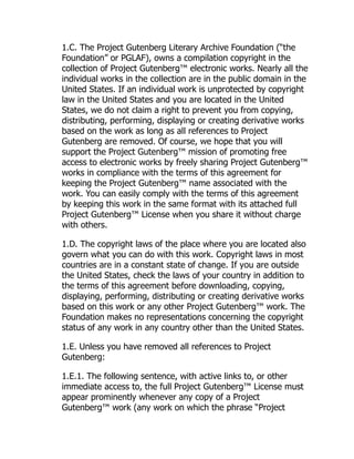
One particular advantage of a rectangular coordinate system over an
oblique one is the calculation of distances. If P and Q are points with
respective rectangular coordinates (x1, y1) and (x2, y2), then we can
introduce the point R which shares its last coordinate with P and its first
with Q—that is, R has coordinates (x2, y1) (see Figure 1.3); then the
triangle with vertices P, Q, and R has a right angle at R. Thus, the line
segment PQ is the hypotenuse, whose length |PQ| is related to the lengths
of the “legs” by Pythagoras’ Theorem
|PQ|2
= |PR|2
+ |RQ|2
.
But the legs are parallel to the axes, so it is easy to see that
|PR| = |△x| = |x2 − x1|
|RQ| = |△y| = |y2 − y1|
and the distance from P to Q is related to their coordinates by
|PQ| =
p
△x2 + △y2 =
p
(x2 − x1)2 + (y2 − y1)2. (1.1)
1
We shall explore some of the differences between rectangular and oblique coordinates
in Exercise 14.
20.
4 CHAPTER 1.COORDINATES AND VECTORS
P R
Q
x1 x2
△x
y1
y2
△y
Figure 1.3: Distance in the Plane
In an oblique system, the formula becomes more complicated (Exercise 14).
Coordinates in Space
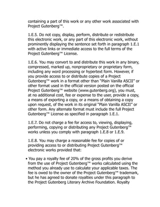
The rectangular coordinate scheme extends naturally to locating points in
space. We again distinguish one point as the origin O, and draw a
horizontal plane through O, on which we construct a rectangular
coordinate system. We continue to call the coordinates in this plane x and
y, and refer to the horizontal plane through the origin as the xy-plane.
Now we draw a new z-axis vertically through O. A point P is located by
first finding the point Pxy in the xy-plane that lies on the vertical line
through P, then finding the signed “height” z of P above this point (z is
negative if P lies below the xy-plane): the rectangular coordinates of P are
the three real numbers (x, y, z), where (x, y) are the coordinates of Pxy in
the rectangular system on the xy-plane. Equivalently, we can define z as
the number corresponding to the intersection of the z-axis with the
horizontal plane through P, which we regard as obtained by moving the
xy-plane “straight up” (or down). Note the standing convention that,
when we draw pictures of space, we regard the x-axis as pointing toward
us (or slightly to our left) out of the page, the y-axis as pointing to the
right in the page, and the z-axis as pointing up in the page (Figure 1.4).
This leads to the identification of the set R3 of triples (x, y, z) of real
numbers with the points of space, which we sometimes refer to as three
dimensional space (or 3-space).
As in the plane, the distance between two points P(x1, y1, z1) and
Q(x2, y2, z2) in R3 can be calculated by applying Pythagoras’ Theorem to
the right triangle PQR, where R(x2, y2, z1) shares its last coordinate with
P and its other coordinates with Q. Details are left to you (Exercise 12);
21.
1.1. LOCATING POINTSIN SPACE 5
x-axis
y-axis
z-axis
P(x, y, z)
z
x
y
Figure 1.4: Pictures of Space
the resulting formula is
|PQ| =
p
△x2 + △y2 + △z2 =
p
(x2 − x1)2 + (y2 − y1)2 + (z2 − z1)2.
(1.2)
In what follows, we will denote the distance between P and Q by
dist(P, Q).
Polar and Cylindrical Coordinates
Rectangular coordinates are the most familiar system for locating points,
but in problems involving rotations, it is sometimes convenient to use a
system based on the direction and distance of a point from the origin.
For points in the plane, this leads to polar coordinates. Given a point P
in the plane, we can locate it relative to the origin O as follows: think of
the line ℓ through P and O as a copy of the real line, obtained by rotating
the x-axis θ radians counterclockwise; then P corresponds to the real
number r on ℓ. The relation of the polar coordinates (r, θ) of P to its
rectangular coordinates (x, y) is illustrated in Figure 1.5, from which we
see that
x = r cos θ
y = r sin θ.
(1.3)
The derivation of Equation (1.3) from Figure 1.5 requires a pinch of salt:
we have drawn θ as an acute angle and x, y, and r as positive. In fact,
when y is negative, our triangle has a clockwise angle, which can be
interpreted as negative θ. However, as long as r is positive, relation (1.3)
22.
6 CHAPTER 1.COORDINATES AND VECTORS
θ
x
y
P
•
ℓ
O
r
→
Figure 1.5: Polar Coordinates
amounts to Euler’s definition of the trigonometric functions (Calculus
Deconstructed, p. 86). To interpret Figure 1.5 when r is negative, we move
|r| units in the opposite direction along ℓ. Notice that a reversal in the
direction of ℓ amounts to a (further) rotation by π radians, so the point
with polar coordinates (r, θ) also has polar coordinates (−r, θ + π).
In fact, while a given geometric point P has only one pair of rectangular
coordinates (x, y), it has many pairs of polar coordinates. Given (x, y), r
can be either solution (positive or negative) of the equation
r2
= x2
+ y2
(1.4)
which follows from a standard trigonometric identity. The angle by which
the x-axis has been rotated to obtain ℓ determines θ only up to adding an
even multiple of π: we will tend to measure the angle by a value of θ
between 0 and 2π or between −π and π, but any appropriate real value is
allowed. Up to this ambiguity, though, we can try to find θ from the
relation
tan θ =
y
x
.
Unfortunately, this determines only the “tilt” of ℓ, not its direction: to
really determine the geometric angle of rotation (given r) we need both
equations
cos θ = x
r
sin θ = y
r .
(1.5)
Of course, either of these alone determines the angle up to a rotation by π
radians (a “flip”), and only the sign in the other equation is needed to
decide between one position of ℓ and its “flip”.
23.
1.1. LOCATING POINTSIN SPACE 7
Thus we see that the polar coordinates (r, θ) of a point P are subject to the
ambiguity that, if (r, θ) is one pair of polar coordinates for P then so are
(r, θ + 2nπ) and (−r, θ + (2n + 1)π) for any integer n (positive or negative).
Finally, we see that r = 0 precisely when P is the origin, so then the line ℓ
is indeterminate: r = 0 together with any value of θ satisfies
Equation (1.3), and gives the origin.
For example, to find the polar coordinates of the point P with rectangular
coordinates (−2
√
3, 2), we first note that
r2
= (−2
√
3)2
+ (2)2
= 16.
Using the positive solution of this
r = 4
we have
cos θ = −
2
√
3
4
= −
√
3
2
sin θ = −
2
4
=
1
2
.
The first equation says that θ is, up to adding multiples of 2π, one of
θ = 5π/6 or θ = 7π/6, while the fact that sin θ is positive picks out the
first value. So one set of polar coordinates for P is
r = 4
θ =
5π
6
+ 2nπ
where n is any integer, while another set is
r = −4
θ =
5π
6
+ π
+ 2nπ
=
11π
6
+ 2nπ.
It may be more natural to write this last expression as
θ = −
π
6
+ 2nπ.
24.
8 CHAPTER 1.COORDINATES AND VECTORS
•
θ
P
•
Pxy
z
r
Figure 1.6: Cylindrical Coordinates
For problems in space involving rotations (or rotational symmetry) about a
single axis, a convenient coordinate system locates a point P relative to
the origin as follows (Figure 1.6): if P is not on the z-axis, then this axis
together with the line OP determine a (vertical) plane, which can be
regarded as the xz-plane rotated so that the x-axis moves θ radians
counterclockwise (in the horizontal plane); we take as our coordinates the
angle θ together with the abcissa and ordinate of P in this plane. The
angle θ can be identified with the polar coordinate of the projection Pxy of
P on the horizontal plane; the abcissa of P in the rotated plane is its
distance from the z-axis, which is the same as the polar coordinate r of
Pxy; and its ordinate in this plane is the same as its vertical rectangular
coordinate z.
We can think of this as a hybrid: combine the polar coordinates (r, θ) of
the projection Pxy with the vertical rectangular coordinate z of P to
obtain the cylindrical coordinates (r, θ, z) of P. Even though in
principle r could be taken as negative, in this system it is customary to
confine ourselves to r ≥ 0. The relation between the cylindrical coordinates
(r, θ, z) and the rectangular coordinates (x, y, z) of a point P is essentially
given by Equation (1.3):
x = r cos θ
y = r sin θ
z = z.
(1.6)
We have included the last relation to stress the fact that this coordinate is
25.
1.1. LOCATING POINTSIN SPACE 9
the same in both systems. The inverse relations are given by (1.4), (1.5)
and the trivial relation z = z.
The name “cylindrical coordinates” comes from the geometric fact that the
locus of the equation r = c (which in polar coordinates gives a circle of
radius c about the origin) gives a vertical cylinder whose axis of symmetry
is the z-axis with radius c.
Cylindrical coordinates carry the ambiguities of polar coordinates: a point
on the z-axis has r = 0 and θ arbitrary, while a point off the z-axis has θ
determined up to adding even multiples of π (since r is taken to be
positive).
For example, the point P with rectangular coordinates (−2
√
3, 2, 4) has
cylindrical coordinates
r = 4
θ =
5π
6
+ 2nπ
z = 4.
Spherical Coordinates
Another coordinate system in space, which is particularly useful in
problems involving rotations around various axes through the origin (for
example, astronomical observations, where the origin is at the center of the
earth) is the system of spherical coordinates. Here, a point P is located
relative to the origin O by measuring the distance of P from the origin
ρ = |OP|
together with two angles: the angle θ between the xz-plane and the plane
containing the z-axis and the line OP, and the angle φ between the
(positive) z-axis and the line OP (Figure 1.7). Of course, the spherical
coordinate θ of P is identical to the cylindrical coordinate θ, and we use
the same letter to indicate this identity. While θ is sometimes allowed to
take on all real values, it is customary in spherical coordinates to restrict φ
to 0 ≤ φ ≤ π. The relation between the cylindrical coordinates (r, θ, z) and
the spherical coordinates (ρ, θ, φ) of a point P is illustrated in Figure 1.8
(which is drawn in the vertical plane determined by θ): 2
2
Be warned that in some of the engineering and physics literature the names of the
two spherical angles are reversed, leading to potential confusion when converting between
spherical and cylindrical coordinates.
26.
10 CHAPTER 1.COORDINATES AND VECTORS
θ
φ
P
•
ρ
Figure 1.7: Spherical Coordinates
P
•
O
z
r
φ
ρ
Figure 1.8: Spherical vs. Cylindrical Coordinates
27.
1.1. LOCATING POINTSIN SPACE 11
r = ρ sin φ
θ = θ
z = ρ cos φ.
(1.7)
To invert these relations, we note that, since ρ ≥ 0 and 0 ≤ φ ≤ π by
convention, z and r completely determine ρ and φ:
ρ =
√
r2 + z2
θ = θ
φ = arccos z
ρ.
(1.8)
The ambiguities in spherical coordinates are the same as those for
cylindrical coordinates: the origin has ρ = 0 and both θ and φ arbitrary;
any other point on the z-axis (φ = 0 or φ = π) has arbitrary θ, and for
points off the z-axis, θ can (in principle) be augmented by arbitrary even
multiples of π.
Thus, the point P with cylindrical coordinates
r = 4
θ =
5π
6
z = 4
has spherical coordinates
ρ = 4
√
2
θ =
5π
6
φ =
π
4
.
Combining Equations (1.6) and (1.7), we can write the relation between
the spherical coordinates (ρ, θ, φ) of a point P and its rectangular
coordinates (x, y, z) as
x = ρ sin φ cos θ
y = ρ sin φ sin θ
z = ρ cos φ.
(1.9)
The inverse relations are a bit more complicated, but clearly, given x, y
and z,
ρ =
p
x2 + y2 + z2 (1.10)
28.
12 CHAPTER 1.COORDINATES AND VECTORS
and φ is completely determined (if ρ 6= 0) by the last equation in (1.9),
while θ is determined by (1.4) and (1.6).
In spherical coordinates, the equation
ρ = R
describes the sphere of radius R centered at the origin, while
φ = α
describes a cone with vertex at the origin, making an angle α (resp. π − α)
with its axis, which is the positive (resp. negative) z-axis if 0 φ π/2
(resp. π/2 φ π).
Exercises for § 1.1
Practice problems:
1. Find the distance between each pair of points (the given coordinates
are rectangular):
(a) (1, 1), (0, 0)
(b) (1, −1), (−1, 1)
(c) (−1, 2), (2, 5)
(d) (1, 1, 1), (0, 0, 0)
(e) (1, 2, 3), (2, 0, −1)
(f) (3, 5, 7), (1, 7, 5)
2. What conditions on the components signify that P(x, y, z)
(rectangular coordinates) belongs to
(a) the x-axis?
(b) the y-axis?
(c) the z-axis?
(d) the xy-plane?
(e) the xz-plane?
(f) the yz-plane?
3. For each point with the given rectangular coordinates, find (i) its
cylindrical coordinates, and (ii) its spherical coordinates:
29.
1.1. LOCATING POINTSIN SPACE 13
(a) x = 0, y = 1,, z = −1
(b) x = 1, y = 1, z = 1
(c) x = 1, y =
√
3, z = 2
(d) x = 1, y =
√
3, z = −2
(e) x = −
√
3, y = 1, z = 1
4. Given the spherical coordinates of the point, find its rectangular
coordinates:
(a) ρ = 2, θ =
π
3
, φ =
π
2
(b) ρ = 1, θ =
π
4
, φ =
2π
3
(c) ρ = 2, θ =
2π
3
, φ =
π
4
(d) ρ = 1, θ =
4π
3
, φ =
π
3
5. What is the geometric meaning of each transformation (described in
cylindrical coordinates) below?
(a) (r, θ, z) → (r, θ, −z)
(b) (r, θ, z) → (r, θ + π, z)
(c) (r, θ, z) → (−r, θ − π
4 , z)
6. Describe the locus of each equation (in cylindrical coordinates) below:
(a) r = 1
(b) θ = π
3
(c) z = 1
7. What is the geometric meaning of each transformation (described in
spherical coordinates) below?
(a) (ρ, θ, φ) → (ρ, θ + π, φ)
(b) (ρ, θ, φ) → (ρ, θ, π − φ)
(c) (ρ, θ, φ) → (2ρ, θ + π
2 , φ)
8. Describe the locus of each equation (in spherical coordinates) below:
(a) ρ = 1
30.
14 CHAPTER 1.COORDINATES AND VECTORS
(b) θ = π
3
(c) φ = π
3
9. Express the plane z = x in terms of (a) cylindrical and (b) spherical
coordinates.
10. What conditions on the spherical coordinates of a point signify that
it lies on
(a) the x-axis?
(b) the y-axis?
(c) the z-axis?
(d) the xy-plane?
(e) the xz-plane?
(f) the yz-plane?
11. A disc in space lies over the region x2 + y2 ≤ a2 (a 0), and the
highest point on the disc has z = b. If P(x, y, z) is a point of the disc,
show that it has cylindrical coordinates satisfying
0 ≤ r ≤ a
0 ≤ θ ≤ 2π
z ≤ b.
Theory problems:
12. Prove the distance formula for R3 (Equation (1.2))
|PQ| =
p
△x2 + △y2 + △z2 =
p
(x2 − x1)2 + (y2 − y1)2 + (z2 − z1)2.
as follows (see Figure 1.9). Given P(x1, y1, z1) and Q(x2, y2, z2), let
R be the point which shares its last coordinate with P and its first
two coordinates with Q. Use the distance formula in R2
(Equation (1.1)) to show that
dist(P, R) =
p
(x2 − x1)2 + (y2 − y1)2,
and then consider the triangle △PRQ. Show that the angle at R is a
right angle, and hence by Pythagoras’ Theorem again,
|PQ| =
q
|PR|2
+ |RQ|2
=
p
(x2 − x1)2 + (y2 − y1)2 + (z2 − z1)2.
31.
1.1. LOCATING POINTSIN SPACE 15
P(x1, y1, z1)
Q(x2, y2, z2)
R(x2, y2, z1)
△z
△x
△y
Figure 1.9: Distance in 3-Space
Challenge problem:
13. Use Pythagoras’ Theorem and the angle-summation formulas to
prove the Law of Cosines: If ABC is any triangle with sides
a = |AC|
b = |BC|
c = |AB|
and the angle at C is ∠ACB = θ, then
c2
= a2
+ b2
− 2ab cos θ. (1.11)
Here is one way to proceed (see Figure 1.10) Drop a perpendicular
a b
x y
z
α β
A B
C
D
Figure 1.10: Law of Cosines
from C to AB, meeting AB at D. This divides the angle at C into
two angles, satisfying
α + β = θ
32.
16 CHAPTER 1.COORDINATES AND VECTORS
and divides AB into two intervals, with respective lengths
|AD| = x
|DB| = y
so
x + y = c.
Finally, set
|CD| = z.
Now show the following:
x = a sin α
y = b sin β
z = a cos α = b cos β
and use this, together with Pythagoras’ Theorem, to conclude that
a2
+ b2
= x2
+ y2
+ 2z2
c2
= x2
+ y2
+ 2xy
and hence
c2
= a2
+ b2
− 2ab cos(α + β).
See Exercise 16 for the version of this which appears in Euclid.
14. Oblique Coordinates: Consider an oblique coordinate system
on R2, in which the vertical axis is replaced by an axis making an
angle of α radians with the horizontal one; denote the corresponding
coordinates by (u, v) (see Figure 1.11).
(a) Show that the oblique coordinates (u, v) and rectangular
coordinates (x, y) of a point are related by
x = u + v cos α
y = v sin α.
33.
1.1. LOCATING POINTSIN SPACE 17
•
P
v
u
u
v
α
Figure 1.11: Oblique Coordinates
(b) Show that the distance of a point P with oblique coordinates
(u, v) from the origin is given by
dist(P, O) =
p
u2 + v2 + 2uv cos α.
(c) Show that the distance between points P (with oblique
coordinates (u1, v1)) and Q (with oblique coordinates (u2, v2)) is
given by
dist(P, Q) =
p
△u2 + △v2 + 2△u△v cos α
where
△u := u2 − u1
△v := v2 − v1.
(Hint: There are two ways to do this. One is to substitute the
expressions for the rectangular coordinates in terms of the
oblique coordinates into the standard distance formula, the
other is to use the law of cosines. Try them both. )
History note:
15. Given a right triangle with “legs” of respective lengths a and b and
hypotenuse of length c (Figure 1.12) Pythagoras’ Theorem says
that
c2
= a2
+ b2
.
In this problem, we outline two quite different proofs of this fact.
First Proof: Consider the pair of figures in Figure 1.13.
(a) Show that the white quadrilateral on the left is a square (that
is, show that the angles at the corners are right angles).
34.
18 CHAPTER 1.COORDINATES AND VECTORS
a
b
c
Figure 1.12: Right-angle triangle
b a
c
b
a
c
b
a
c
b
a c
a b
a
b
Figure 1.13: Pythagoras’ Theorem by Dissection
(b) Explain how the two figures prove Pythagoras’ theorem.
A variant of Figure 1.13 was used by the twelfth-century Indian
writer Bhāskara (b. 1114) to prove Pythagoras’ Theorem. His proof
consisted of a figure related to Figure 1.13 (without the shading)
together with the single word “Behold!”.
According to Eves [15, p. 158] and Maor [37, p. 63], reasoning based
on Figure 1.13 appears in one of the oldest Chinese mathematical
manuscripts, the Caho Pei Suang Chin, thought to date from the
Han dynasty in the third century B.C.
The Pythagorean Theorem appears as Proposition 47, Book I of
Euclid’s Elements with a different proof (see below). In his
translation of the Elements, Heath has an extensive commentary on
this theorem and its various proofs [29, vol. I, pp. 350-368]. In
particular, he (as well as Eves) notes that the proof above has been
suggested as possibly the kind of proof that Pythagoras himself
might have produced. Eves concurs with this judgement, but Heath
does not.
Second Proof: The proof above represents one tradition in proofs
of the Pythagorean Theorem, which Maor [37] calls “dissection
proofs.” A second approach is via the theory of proportions. Here is
35.
1.1. LOCATING POINTSIN SPACE 19
an example: again, suppose △ABC has a right angle at C; label the
sides with lower-case versions of the labels of the opposite vertices
(Figure 1.14) and draw a perpendicular CD from the right angle to
the hypotenuse. This cuts the hypotenuse into two pieces of
respective lengths c1 and c2, so
c = c1 + c2. (1.12)
Denote the length of CD by x.
D
C A
B
a
b
x
c1
c2
Figure 1.14: Pythagoras’ Theorem by Proportions
(a) Show that the two triangles △ACD and △CBD are both
similar to △ABC.
(b) Using the similarity of △CBD with △ABC, show that
a
c
=
c1
a
or
a2
= cc1.
(c) Using the similarity of △ACD with △ABC, show that
c
b
=
b
c2
or
b2
= cc2.
36.
20 CHAPTER 1.COORDINATES AND VECTORS
(d) Now combine these equations with Equation (1.12) to prove
Pythagoras’ Theorem.
The basic proportions here are those that appear in Euclid’s proof of
Proposition 47, Book I of the Elements , although he arrives at these
via different reasoning. However, in Book VI, Proposition 31 , Euclid
presents a generalization of this theorem: draw any polygon using
the hypotenuse as one side; then draw similar polygons using the legs
of the triangle; Proposition 31 asserts that the sum of the areas of
the two polygons on the legs equals that of the polygon on the
hypotenuse. Euclid’s proof of this proposition is essentially the
argument given above.
16. The Law of Cosines for an acute angle is essentially given by
Proposition 13 in Book II of Euclid’s Elements[29, vol. 1, p. 406] :
In acute-angled triangles the square on the side subtending
the acute angle is less than the squares on the sides
containing the acute angle by twice the rectangle contained
by one of the sides about the acute angle, namely that on
which the perpendicular falls, and the straight line cut off
within by the perpendicular towards the acute angle.
Translated into algebraic language (see Figure 1.15, where the acute
angle is ∠ABC) this says
A
B C
D
Figure 1.15: Euclid Book II, Proposition 13
|AC|2
= |CB|2
+ |BA|2
− |CB| |BD| .
Explain why this is the same as the Law of Cosines.
1.2 Vectors and Their Arithmetic
Many quantities occurring in physics have a magnitude and a
direction—for example, forces, velocities, and accelerations. As a
37.
1.2. VECTORS ANDTHEIR ARITHMETIC 21
prototype, we will consider displacements.
Suppose a rigid body is pushed (without being rotated) so that a
distinguished spot on it is moved from position P to position Q
(Figure 1.16). We represent this motion by a directed line segment, or
arrow, going from P to Q and denoted
−
−
→
PQ. Note that this arrow encodes
all the information about the motion of the whole body: that is, if we had
distinguished a different spot on the body, initially located at P′, then its
motion would be described by an arrow
−
−
→
P′Q′ parallel to
−
−
→
PQ and of the
same length: in other words, the important characteristics of the
displacement are its direction and magnitude, but not the location in space
of its initial or terminal points (i.e., its tail or head).
P
Q
Figure 1.16: Displacement
A second important property of displacement is the way different
displacements combine. If we first perform a displacement moving our
distinguished spot from P to Q (represented by the arrow
−
−
→
PQ) and then
perform a second displacement moving our spot from Q to R (represented
by the arrow
−
−
→
QR), the net effect is the same as if we had pushed directly
from P to R. The arrow
−
→
PR representing this net displacement is formed
by putting arrow
−
−
→
QR with its tail at the head of
−
−
→
PQ and drawing the
arrow from the tail of
−
−
→
PQ to the head of
−
−
→
QR (Figure 1.17). More
generally, the net effect of several successive displacements can be found by
forming a broken path of arrows placed tail-to-head, and forming a new
arrow from the tail of the first arrow to the head of the last.
A representation of a physical (or geometric) quantity with these
characteristics is sometimes called a vectorial representation. With
respect to velocities, the “parallelogram of velocities” appears in the
Mechanica, a work incorrectly attributed to, but contemporary with,
38.
22 CHAPTER 1.COORDINATES AND VECTORS
Figure 1.17: Combining Displacements
Aristotle (384-322 BC) [26, vol. I, p. 344], and is discussed at some length
in the Mechanics by Heron of Alexandria (ca. 75 AD) [26, vol. II, p. 348].
The vectorial nature of some physical quantities, such as velocity,
acceleration and force, was well understood and used by Isaac Newton
(1642-1727) in the Principia [41, Corollary 1, Book 1 (p. 417)]. In the late
eighteenth and early nineteenth century, Paolo Frisi (1728-1784), Leonard
Euler (1707-1783), Joseph Louis Lagrange (1736-1813), and others realized
that other physical quantities, associated with rotation of a rigid body
(torque, angular velocity, moment of a force), could also be usefully given
vectorial representations; this was developed further by Louis Poinsot
(1777-1859), Siméon Denis Poisson (1781-1840), and Jacques Binet
(1786-1856). At about the same time, various geometric quantities (e.g.,
areas of surfaces in space) were given vectorial representations by Gaetano
Giorgini (1795-1874), Simon Lhuilier (1750-1840), Jean Hachette
(1769-1834), Lazare Carnot (1753-1823)), Michel Chasles (1793-1880) and
later by Hermann Grassmann (1809-1877) and Giuseppe Peano
(1858-1932). In the early nineteenth century, vectorial representations of
complex numbers (and their extension, quaternions) were formulated by
several researchers; the term vector was coined by William Rowan
Hamilton (1805-1865) in 1853. Finally, extensive use of vectorial properties
of electromagnetic forces was made by James Clerk Maxwell (1831-1879)
and Oliver Heaviside (1850-1925) in the late nineteenth century. However,
a general theory of vectors was only formulated in the very late nineteenth
39.
1.2. VECTORS ANDTHEIR ARITHMETIC 23
century; the first elementary exposition was given by Edwin Bidwell
Wilson (1879-1964) in 1901 [57], based on lectures by the American
mathematical physicist Josiah Willard Gibbs (1839-1903)3 [19].
By a geometric vector in R3 (or R2) we will mean an “arrow” which can
be moved to any position, provided its direction and length are
maintained.4 We will denote vectors with a letter surmounted by an arrow,
like this: −
→
v . We define two operations on vectors. The sum of two vectors
is formed by moving −
→
w so that its “tail” coincides in position with the
“head” of −
→
v , then forming the vector −
→
v + −
→
w whose tail coincides with
that of −
→
v and whose head coincides with that of −
→
w (Figure 1.18). If
−
→
v
−
→
w
−
→
v
+
−
→
w
Figure 1.18: Sum of two vectors
instead we place −
→
w with its tail at the position previously occupied by the
tail of −
→
v and then move −
→
v so that its tail coincides with the head of −
→
w ,
we form −
→
w + −
→
v , and it is clear that these two configurations form a
parallelogram with diagonal
−
→
v + −
→
w = −
→
w + −
→
v
(Figure G.1). This is the commutative property of vector addition.
A second operation is scaling or multiplication of a vector by a
number. We naturally define
1−
→
v = −
→
v
2−
→
v = −
→
v + −
→
v
3−
→
v = −
→
v + −
→
v + −
→
v = 2−
→
v + −
→
v
and so on, and then define rational multiples by
−
→
v =
m
n
−
→
w ⇔ n−
→
v = m−
→
w;
3
I learned much of this from Sandro Caparrini [6, 7, 8]. This narrative differs from the
standard one, given by Michael Crowe [11]
4
This mobility is sometimes expressed by saying it is a free vector.
40.
24 CHAPTER 1.COORDINATES AND VECTORS
−
→
v
−
→
w
−
→
v
−
→
w
−
→
v
+
−
→
w
−
→
w
+
−
→
v
Figure 1.19: Parallelogram Rule (Commutativity of Vector Sums)
finally, suppose
mi
ni
→ ℓ
is a convergent sequence of rationals. For any fixed vector −
→
v , if we draw
arrows representing the vectors (mi/ni)−
→
v with all their tails at a fixed
position, then the heads will form a convergent sequence of points along a
line, whose limit is the position for the head of ℓ−
→
v . Alternatively, if we
pick a unit of length, then for any vector −
→
v and any positive real number
r, the vector r−
→
v has the same direction as −
→
v , and its length is that of −
→
v
multiplied by r. For this reason, we refer to real numbers (in a vector
context) as scalars.
If
−
→
u = −
→
v + −
→
w
then it is natural to write
−
→
v = −
→
u − −
→
w
and from this (Figure 1.20) it is natural to define the negative −−
→
w of a
vector −
→
w as the vector obtained by interchanging the head and tail of −
→
w .
This allows us to also define multiplication of a vector −
→
v by any negative
real number r = − |r| as
(− |r|)−
→
v := |r| (−−
→
v )
—that is, we reverse the direction of −
→
v and “scale” by |r|.
Addition of vectors (and of scalars) and multiplication of vectors by scalars
have many formal similarities with addition and multiplication of numbers.
We list the major ones (the first of which has already been noted above):
• Addition of vectors is
commutative: −
→
v + −
→
w = −
→
w + −
→
v , and
41.
1.2. VECTORS ANDTHEIR ARITHMETIC 25
−
→
v
−
→
w
−
→
u
−
→
v
-−
→
w
−
→
u
−
→
u = −
→
v + −
→
w −
→
v = −
→
u − −
→
w
Figure 1.20: Difference of vectors
associative: −
→
u + (−
→
v + −
→
w ) = (−
→
u + −
→
v ) + −
→
w .
• Multiplication of vectors by scalars
distributes over vector sums: r(−
→
v + −
→
w ) = r−
→
w + r−
→
v , and
distributes over scalar sums: (r + s)−
→
v = r−
→
v + s−
→
v .
We will explore some of these properties further in Exercise 3.
The interpretation of displacements as vectors gives us an alternative way
to represent vectors. We will say that an arrow representing the vector −
→
v
is in standard position if its tail is at the origin. Note that in this case
the vector is completely determined by the position of its head, giving us a
natural correspondence between vectors −
→
v in R3 (or R2) and points
P ∈ R3 (resp. R2). −
→
v corresponds to P if the arrow
−
−
→
OP from the origin to
P is a representation of −
→
v : that is, −
→
v is the vector representing that
displacement of R3 which moves the origin to P; we refer to −
→
v as the
position vector of P. We shall make extensive use of the correspondence
between vectors and points, often denoting a point by its position vector
−
→
p ∈ R3.
Furthermore, using rectangular coordinates we can formulate a numerical
specification of vectors in which addition and multiplication by scalars is
very easy to calculate: if −
→
v =
−
−
→
OP and P has rectangular coordinates
(x, y, z), we identify the vector −
→
v with the triple of numbers (x, y, z) and
write −
→
v = (x, y, z). We refer to x, y and z as the components or entries
of −
→
v . Then if −
→
w =
−
−
→
OQ where Q = (△x, △y, △z) (that is,
−
→
w = (△x, △y, △z)), we see from Figure 1.21 that
−
→
v + −
→
w = (x + △x, y + △y, z + △z);
that is, we add vectors componentwise.
42.
26 CHAPTER 1.COORDINATES AND VECTORS
O
−
→
v
P(x, y, z)
−
→
w
−
→
v
+
−
→
w
Q(△x, △y, △z)
−
→
w
Figure 1.21: Componentwise addition of vectors
Similarly, if r is any scalar and −
→
v = (x, y, z), then
r−
→
v = (rx, ry, rz) :
a scalar multiplies all entries of the vector.
This representation points out the presence of an exceptional vector—the
zero vector
−
→
0 := (0, 0, 0)
which is the result of either multiplying an arbitrary vector by the scalar
zero
0−
→
v =
−
→
0
or of subtracting an arbitrary vector from itself
−
→
v − −
→
v =
−
→
0 .
As a point,
−
→
0 corresponds to the origin O itself. As an “arrow”, its tail
and head are at the same position. As a displacement, it corresponds to
not moving at all. Note in particular that the zero vector does not have a
well-defined direction—a feature which will be important to remember in
the future. From a formal, algebraic point of view, the zero vector plays
the role for vector addition that is played by the number zero for addition
of numbers: it is an additive identity element, which means that
adding it to any vector gives back that vector:
−
→
v +
−
→
0 = −
→
v =
−
→
0 + −
→
v .
A final feature that is brought out by thinking of vectors in R3 as triples of
numbers is that we can recover the entries of a vector geometrically. Note
43.
1.2. VECTORS ANDTHEIR ARITHMETIC 27
that if −
→
v = (x, y, z) then we can write
−
→
v = (x, 0, 0) + (0, y, 0) + (0, 0, z)
= x(1, 0, 0) + y(0, 1, 0) + z(0, 0, 1).
This means that any vector in R3 can be expressed as a sum of scalar
multiples (or linear combination) of three specific vectors, known as the
standard basis for R3, and denoted
−
→
ı = (1, 0, 0)
−
→
= (0, 1, 0)
−
→
k = (0, 0, 1).
It is easy to see that these are the vectors of length 1 pointing along the
three (positive) coordinate axes (see Figure 1.22). Thus, every vector
x
y
z
−
→
ı −
→
−
→
k
−
→
v
(x)−
→
ı
(y)−
→
(z)
−
→
k
Figure 1.22: The Standard Basis for R3
−
→
v ∈ R3 can be expressed as
−
→
v = x−
→
ı + y−
→
+ z
−
→
k .
We shall find it convenient to move freely between the coordinate notation
−
→
v = (x, y, z) and the “arrow” notation −
→
v = x−
→
ı + y−
→
+ z
−
→
k ; generally, we
adopt coordinate notation when −
→
v is regarded as a position vector, and
“arrow” notation when we want to picture it as an arrow in space.
We began by thinking of a vector −
→
v in R3 as determined by its magnitude
and its direction, and have ended up thinking of it as a triple of numbers.
44.
28 CHAPTER 1.COORDINATES AND VECTORS
To come full circle, we recall that the vector −
→
v = (x, y, z) has as its
standard representation the arrow
−
−
→
OP from the origin O to the point P
with coordinates (x, y, z); thus its magnitude (or length, denoted −
→
v ) is
given by the distance formula
|−
→
v | =
p
x2 + y2 + z2.
When we want to specify the direction of −
→
v , we “point”, using as our
standard representation the unit vector—that is, the vector of length
1—in the direction of −
→
v . From the scaling property of multiplication by
real numbers, we see that the unit vector in the direction of a vector −
→
v
(−
→
v 6=
−
→
0 ) is
u(−
→
v ) =
1
|−
→
v |
−
→
v .
In particular, the standard basis vectors −
→
ı , −
→
, and
−
→
k are unit vectors
along the (positive) coordinate axes.
This formula for unit vectors gives us an easy criterion for deciding
whether two vectors point in parallel directions. Given (nonzero5) vectors
−
→
v and −
→
w , the respective unit vectors in the same direction are
u(−
→
v ) =
1
|−
→
v |
−
→
v
u(−
→
w ) =
1
|−
→
w |
−
→
w .
The two vectors −
→
v and −
→
w point in the same direction precisely if the two
unit vectors are equal
u(−
→
v ) = u(−
→
w ) = −
→
u
or
−
→
v = |−
→
v | −
→
u
−
→
w = |−
→
w | −
→
u .
This can also be expressed as
−
→
v = λ−
→
w
−
→
w =
1
λ
−
→
v
5
A vector is nonzero if it is not equal to the zero vector. Thus, some of its entries
can be zero, but not all of them.
45.
1.2. VECTORS ANDTHEIR ARITHMETIC 29
where the (positive) scalar λ is
λ =
|−
→
v |
|−
→
w |
.
Similarly, the two vectors point in opposite directions if the two unit
vectors are negatives of each other, or
−
→
v = λ−
→
w
−
→
w =
1
λ
−
→
v
where the negative scalar λ is
λ = −
|−
→
v |
|−
→
w |
.
So we have shown
Remark 1.2.1. For two nonzero vectors −
→
v = (x1, y1, z1) and
−
→
w = (x2, y2, z2), the following are equivalent:
• −
→
v and −
→
w point in parallel or opposite directions;
• −
→
v = λ−
→
w for some nonzero scalar λ;
• −
→
w = λ′−
→
v for some nonzero scalar λ′;
•
x1
x2
=
y1
y2
=
z1
z2
= λ for some nonzero scalar λ (where if one of the
entries of −
→
w is zero, so is the corresponding entry of −
→
v , and the
corresponding ratio is omitted from these equalities.)
•
x2
x1
=
y2
y1
=
z2
z1
= λ′
for some nonzero scalar λ′ (where if one of the
entries of −
→
w is zero, so is the corresponding entry of −
→
v , and the
corresponding ratio is omitted from these equalities.)
The values of λ (resp. λ′) are the same wherever they appear above, and λ′
is the reciprocal of λ.
λ (hence also λ′) is positive precisely if −
→
v and −
→
w point in the same
direction, and negative precisely if they point in opposite directions.
46.
30 CHAPTER 1.COORDINATES AND VECTORS
Two (nonzero) vectors are linearly dependent if they point in either the
same or opposite directions—that is, if we picture them as arrows from a
common initial point, then the two heads and the common tail fall on a
line (this terminology will be extended in Exercise 7—but for more than
two vectors, the condition is more complicated). Vectors which are not
linearly dependent are linearly independent.
Exercises for § 1.2
Practice problems:
1. In each part, you are given two vectors, −
→
v and −
→
w . Find (i) −
→
v + −
→
w ;
(ii) −
→
v − −
→
w ; (iii) 2−
→
v ; (iv) 3−
→
v − 2−
→
w ; (v) the length of −
→
v , k−
→
v k;
(vi) the unit vector −
→
u in the direction of −
→
v :
(a) −
→
v = (3, 4), −
→
w = (−1, 2)
(b) −
→
v = (1, 2, −2), −
→
w = (2, −1, 3)
(c) −
→
v = 2−
→
ı − 2−
→
−
−
→
k , −
→
w = 3−
→
ı + −
→
− 2
−
→
k
2. In each case below, decide whether the given vectors are linearly
dependent or linearly independent.
(a) (1, 2), (2, 4)
(b) (1, 2), (2, 1)
(c) (−1, 2), (3, −6)
(d) (−1, 2), (2, 1)
(e) (2, −2, 6), (−3, 3, 9)
(f) (−1, 1, 3), (3, −3, −9)
(g) −
→
ı + −
→
+
−
→
k , 2−
→
ı − 2−
→
+ 2
−
→
k
(h) 2−
→
ı − 4−
→
+ 2
−
→
k , −−
→
ı + 2−
→
−
−
→
k
Theory problems:
3. (a) We have seen that the commutative property of vector addition
can be interpreted via the “parallelogram rule” (Figure G.1).
Give a similar pictorial interpretation of the associative
property.
(b) Give geometric arguments for the two distributive properties of
vector arithmetic.
47.
1.2. VECTORS ANDTHEIR ARITHMETIC 31
(c) Show that if
a−
→
v =
−
→
0
then either
a = 0
or
−
→
v =
−
→
0 .
(Hint: What do you know about the relation between lengths
for −
→
v and a−
→
v ?)
(d) Show that if a vector −
→
v satisfies
a−
→
v = b−
→
v
where a 6= b are two specific, distinct scalars, then −
→
v =
−
→
0 .
(e) Show that vector subtraction is not associative.
4. Polar notation for vectors:
(a) Show that any planar vector −
→
u of length 1 can be written in
the form
−
→
u = (cos θ, sin θ)
where θ is the (counterclockwise) angle between −
→
u and the
positive x-axis.
(b) Conclude that every nonzero planar vector −
→
v can be expressed
in polar form
−
→
v = |−
→
v | (cos θ, sin θ)
where θ is the (counterclockwise) angle between −
→
v and the
positive x-axis.
5. (a) Show that if −
→
v and −
→
w are two linearly independent vectors in
the plane, then every vector in the plane can be expressed as a
linear combination of −
→
v and −
→
w . (Hint: The independence
assumption means they point along non-parallel lines. Given a
point P in the plane, consider the parallelogram with the origin
and P as opposite vertices, and with edges parallel to −
→
v and −
→
w .
Use this to construct the linear combination.)
48.
32 CHAPTER 1.COORDINATES AND VECTORS
(b) Now suppose −
→
u , −
→
v and −
→
w are three nonzero vectors in R3. If
−
→
v and −
→
w are linearly independent, show that every vector lying
in the plane that contains the two lines through the origin
parallel to −
→
v and −
→
w can be expressed as a linear combination
of −
→
v and −
→
w . Now show that if −
→
u does not lie in this plane,
then every vector in R3 can be expressed as a linear
combination of −
→
u , −
→
v and −
→
w .
The two statements above are summarized by saying that −
→
v and −
→
w
(resp. −
→
u , −
→
v and −
→
w ) span R2 (resp. R3).
Challenge problem:
6. Show (using vector methods) that the line segment joining the
midpoints of two sides of a triangle is parallel to and has half the
length of the third side.
7. Given a collection {−
→
v1, −
→
v2, . . . , −
→
vk} of vectors, consider the equation
(in the unknown coefficients c1,. . . ,ck)
c1
−
→
v1 + c2
−
→
v2 + · · · + ck
−
→
vk =
−
→
0 ; (1.13)
that is, an expression for the zero vector as a linear combination of
the given vectors. Of course, regardless of the vectors −
→
vi , one
solution of this is
c1 = c2 = · · · = 0;
the combination coming from this solution is called the trivial
combination of the given vectors. The collection {−
→
v1, −
→
v2, . . . , −
→
vk} is
linearly dependent if there exists some nontrivial combination of
these vectors—that is, a solution of Equation (1.13) with at least one
nonzero coefficient. It is linearly independent if it is not linearly
dependent—that is, if the only solution of Equation (1.13) is the
trivial one.
(a) Show that any collection of vectors which includes the zero
vector is linearly dependent.
(b) Show that a collection of two nonzero vectors {−
→
v1, −
→
v2} in R3 is
linearly independent precisely if (in standard position) they
point along non-parallel lines.
(c) Show that a collection of three position vectors in R3 is linearly
dependent precisely if at least one of them can be expressed as a
linear combination of the other two.
49.
1.3. LINES INSPACE 33
(d) Show that a collection of three position vectors in R3 is linearly
independent precisely if the corresponding points determine a
plane in space that does not pass through the origin.
(e) Show that any collection of four or more vectors in R3 is
linearly dependent. (Hint: Use either part (a) of this problem or
part (b) of Exercise 5.)
1.3 Lines in Space
Parametrization of Lines
A line in the plane is the locus of a “linear” equation in the rectangular
coordinates x and y
Ax + By = C
where A, B and C are real constants with at least one of A and B nonzero.
A geometrically informative version of this is the slope-intercept
formula for a non-vertical line
y = mx + b (1.14)
where the slope m is the tangent of the angle the line makes with the
horizontal and the y-intercept b is the ordinate (signed height) of its
intersection with the y-axis.
Unfortunately, neither of these schemes extends verbatim to a
three-dimensional context. In particular, the locus of a “linear” equation
in the three rectangular coordinates x, y and z
Ax + By + Cz = D
is a plane, not a line. Fortunately, though, we can use vectors to
implement the geometric thinking behind the point-slope formula (1.14).
This formula separates two pieces of geometric data which together
determine a line: the slope reflects the direction (or tilt) of the line, and
then the y-intercept distinguishes between the various parallel lines with a
given slope by specifying a point which must lie on the line. A direction in
3-space cannot be determined by a single number, but it is naturally
specified by a nonzero vector, so the three-dimensional analogue of the
slope of a line is a direction vector
−
→
v = a−
→
ı + b−
→
+ c
−
→
k
50.
34 CHAPTER 1.COORDINATES AND VECTORS
to which it is parallel.6 Then, to pick out one among all the lines parallel
to −
→
v , we specify a basepoint P0(x0, y0, z0) through which the line is
required to pass.
The points lying on the line specified by a particular direction vector −
→
v
and basepoint P0 are best described in terms of their position vectors.
Denote the position vector of the basepoint by
−
→
p0 = x0
−
→
ı + y0
−
→
+ z0
−
→
k ;
then to reach any other point P(x, y, z) on the line, we travel parallel to −
→
v
from P0, which is to say the displacement
−
−
→
P0P from P0 is a scalar multiple
of the direction vector:
−
−
→
P0P = t−
→
v .
The position vector −
→
p (t) of the point corresponding to this scalar multiple
of −
→
v is
−
→
p (t) = −
→
p0 + t−
→
v
which defines a vector-valued function of the real variable t. In terms of
coordinates, this reads
x = x0 + at
y = y0 + bt
z = z0 + ct.
We refer to the vector-valued function −
→
p (t) as a parametrization; the
coordinate equations are parametric equations for the line.
The vector-valued function −
→
p (t) can be interpreted kinematically: it gives
the position vector at time t of the moving point whose position at time
t = 0 is the basepoint P0, and which is travelling at the constant velocity
−
→
v . Note that to obtain the full line, we need to consider negative as well
as positive values of t—that is, the domain of the function −
→
p (t) is the
whole real line, −∞ t ∞.
It is useful to keep in mind the distinction between the parametrization
−
→
p (t), which represents a moving point, and the line ℓ being parametrized,
which is the path of this moving point. A given line ℓ has many different
parametrizations: we can take any point on ℓ as P0, and any nonzero
vector pointing parallel to ℓ as the direction vector −
→
v . This ambiguity
means we need to be careful when making geometric comparisons between
6
In general, we do not need to restrict ourselves to unit direction vectors; any nonzero
vector will do.
51.
1.3. LINES INSPACE 35
lines given parametrically. Nonetheless, this way of presenting lines
exhibits geometric information in a very accessible form.
For example, let us consider two lines in 3-space. The first, ℓ1, is given by
the parametrization
−
→
p1(t) = (1, −2, 3) + t(−3, −2, 1)
or, in coordinate form,
x = 1 −3t
y = −2 −2t
z = 3 +t
while the second, ℓ2, is given in coordinate form as
x = 1 +6t
y = 4t
z = 1 −2t.
We can easily read off from this that ℓ2 has parametrization
−
→
p2(t) = (1, 0, 1) + t(6, 4, −2).
Comparing the two direction vectors
−
→
v1 = −3−
→
ı − 2−
→
+
−
→
k
−
→
v2 = 6−
→
ı + 4−
→
− 2
−
→
k
we see that
−
→
v2 = −2−
→
v1
so the two lines have the same direction—either they are parallel, or they
coincide. To decide which is the case, it suffices to decide whether the
basepoint of one of the lines lies on the other line. Let us see whether the
basepoint of ℓ2
−
→
p2(0) = (1, 0, 1)
lies on ℓ1. This means we need to see if for some value of t we have
−
→
p2(0) = −
→
p1(t), or
1 = 1 −3t
0 = −2 −2t
1 = 3 +t.
52.
36 CHAPTER 1.COORDINATES AND VECTORS
It is easy to see that the first equation requires t = 0, the second requires
t = −1, and the third requires t = −2; there is no way we can solve all
three simultaneously. It follows that ℓ1 and ℓ2 are distinct, but parallel,
lines.
Now, consider a third line, ℓ3, given by
x = 1 +3t
y = 2 +t
z = −3 +t.
We read off its direction vector as
−
→
v3 = 3−
→
ı + −
→
+
−
→
k
which is clearly not a scalar multiple of the other two. This tells us
immediately that ℓ3 is different from both ℓ1 and ℓ2 (it has a different
direction). Let us ask whether ℓ2 intersects ℓ3. It might be tempting to try
to answer this by looking for a solution of the vector equation
−
→
p2(t) = −
→
p3(t)
but this would be a mistake. Remember that these two parametrizations
describe the positions of two points—one moving along ℓ2 and the other
moving along ℓ3—at time t. The equation above requires the two points to
be at the same place at the same time—in other words, it describes a
collision. But all we ask is that the two paths cross: it would suffice to
locate a place occupied by both moving points, but possibly at different
times. This means we need to distinguish the parameters appearing in the
two functions −
→
p2(t) and −
→
p3(t), by renaming one of them (say the first) as
(say) s: the vector equation we need to solve is
−
→
p2(s) = −
→
p3(t) ,
which amounts to the three equations in two unknowns
1 +6s = 1 +3t
4s = 2 +t
1 −2s = −3 +t.
The first equation can be reduced to the condition
2s = t
53.
1.3. LINES INSPACE 37
and substituting this into the other two equations
2t = 2 +t
1 −t = −3 +t
we end up with the solution
t = 2
s = 1
—that is, the lines ℓ2 and ℓ3 intersect at the point
−
→
p2(1) = (7, 4, −1) = −
→
p3(2) .
Now let us apply the same process to see whether ℓ1 intersects ℓ3. The
vector equation
−
→
p1(s) = −
→
p3(t)
yields the three coordinate equations
1 −3s = 1 +3t
−2 −2s = 2 +t
3 +s = −3 +t.
You can check that these imply, respectively
s = −t
−2s = 4 +t
s = −6 +t.
Substituting the first equality into the other two yields, respectively
2t = 4 +t
−t = −6 +t
and the only value of t for which the first (resp. second) holds is,
respectively,
t = 4
t = 3.
Thus our three coordinate equations cannot be satisfied simultaneously; it
follows that ℓ1 and ℓ3 do not intersect, even though they are not parallel.
Such lines are sometimes called skew lines .
54.
38 CHAPTER 1.COORDINATES AND VECTORS
Geometric Applications
A basic geometric fact is that any pair of distinct points determines a line.
Given two points P1(x1, y1, z1) and P2(x2, y2, z2), how do we find a
parametrization of the line ℓ they determine?
Suppose the position vectors of the two points are
−
→
p1 = x1
−
→
ı + y1
−
→
+ z1
−
→
k
−
→
p2 = x2
−
→
ı + y2
−
→
+ z2
−
→
k .
The vector
−
−
−
→
P1P2 joining them lies along ℓ, so we can use it as a direction
vector:
−
→
v = −
→
p2 − −
→
p1 = △x−
→
ı + △y−
→
+ △z
−
→
k
where △x = x2 − x1, △y = y2 − y1, and △z = z2 − z1. Using P1 as
basepoint, this leads to the parametrization
−
→
p (t) = −
→
p1 + t−
→
v
= −
→
p1 + t(−
→
p2 − −
→
p1)
= (1 − t)−
→
p1 + t−
→
p2.
Note that we have set this up so that
−
→
p (0) = −
→
p1
−
→
p (1) = −
→
p2.
The full line ℓ through these points corresponds to allowing the parameter
to take on all real values. However, if we restrict t to the interval
0 ≤ t ≤ 1, the corresponding points fill out the line segment P1P2. Since
the point −
→
p (t) is travelling with constant velocity, we have the following
observations:
Remark 1.3.1 (Two-Point Formula). Suppose P1(x1, y1, z1) and
P2(x2, y2, z2) are distinct points. The line through P1 and P2 is given by
the parametrization7
−
→
p (t) = (1 − t)−
→
p1 + t−
→
p2
7
This is the parametrized form of the two-point formula for a line in the plane
determined by a pair of points.
And of fourdozen Chairs for Board Room
use, for the sum of
76 16 0
November 20.
(8.)
A Contract or Agreement with William
Druce and Son for the supply from time to
time of the best Wall’s End Coal, at per ton
24s.
And of the best Gas Coke, at per chaldron
13s.
Expires Midsummer, 1861.
December 18.
(3.)
A Contract or Agreement with the
Manchester Fife Assurance Office for an
Insurance of the Fixtures, Fittings, and
Furniture in this Building, to the amount of
£700, at an annual payment at Christmas
of
1 15 0
December 18.
(4.)
A Contract or Agreement with the Union
Assurance Office for an Insurance of the
Vestry Hall Building to the amount of
£6000 (superseding that of June, 1860), at
an annual payment of
16 10 0
December 18.
(12.)
A Contract or Agreement with the Council
of the Chelsea Literary and Scientific
Institution for the use of a portion of the
Vestry Hall Building, lighted, warmed, c.,
c., at a yearly Rent of
Terminable at six months’ notice on either
side.
50 0 0
1861.
January 1. (6.) A Contract or Agreement with Parsons,
Brothers, to execute Plumbers’ Work at
fixed prices, on demand.
Expires Midsummer, 1861.
57.
January 1. (10.)A Contract with H. D. Pite and Son for
General Printing, at fixed prices, on
demand.
Expires 30th June, 1861.
January 1. (11.) A Contract or Agreement with W. Davis for
the supply of Scavengers’ Brooms, at a
fixed price, on demand.
Expires Midsummer, 1861.
February 12.
(10.)
A Contract with Ann Emmerson for
watering (for the season) the Streets of,
and for the removal of the Slop, c., from,
that portion of the Parish North of the
King’s Road (exclusive of Kensal New
Town), for the sum of
Expires March 1, 1862.
740 0 0
February 12.
(12.)
A Contract with Charles Hornsby for
watering (for the season) the Streets of,
and for the removal of the Slop, c., from,
that portion of the Parish South of, and
including, the King’s Road, for the sum of
Expires 1st March, 1862.
625 0 0
February 12.
(12.)
A Contract with Ann Emmerson for the
supply of Horses, Carts, and Drivers, as
may be required in any part of the Parish,
at fixed prices, on demand.
Expires 1st March, 1862.
February 12.
(14.)
A Contract or Agreement with Messrs.
Nicholls, Brothers, for Repairing, and
keeping in Repair, the Public Pumps, for
the sum of
Expires 1st March, 1862.
26 10 0
58.
February 26.
(9.)
A Contractwith Thomas Edmonds for
watering the Roads of Kensal New Town
(for the season), and for the removal of
Slop, c., from the same throughout the
year, for the sum of
Expires 1st March, 1862.
90 0 0
59.
APPENDIX No. 41.
BYELAWS.
The Vestry of the Parish of Chelsea, in the County of Middlesex.
Part I.
For Regulating the Business Proceedings at Vestry Meetings.
1. Two clear days’ notice of every alternate Vestry Meeting (as
hereinafter explained) shall be sent by the Vestry Clerk to each
Vestryman, at his usual or last known place of abode; and such
notice shall state the time and place of such meeting, and the
business to be transacted, so far as the same is known, in its
appointed order. Provided that whenever the period of adjournment
renders two days’ notice impracticable, notice shall be sent as early
as possible.
2. Meetings of the Vestry shall be held every Tuesday at three o’clock
in the afternoon. But the Vestrymen shall be summoned only for
every alternate Tuesday for general business. The business to be
done at the other meetings to be confined to the issuing of orders
for promoting the construction of works under the 76th Section of
the Act, 18th and 19th Vic., cap. 120; unless at any previous
meeting a resolution be adopted to make the meeting special for the
discussion of a particular subject.
3. Every Vestryman, before taking part in any business at a Vestry
Meeting, shall sign his name in the Vestrymen’s Attendance Book, to
60.
be placed atthe entrance for that purpose.
4. If at the end of half an hour from the time stated in the Notice
convening the Meeting there should not be nine Vestrymen present,
the meeting shall stand adjourned until the following Tuesday, and
the Clerk shall give notice accordingly.
5. The Chairman shall be elected at the precise hour stated in the
notice, or as soon as Nine Vestrymen are present; and the first
business at ordinary meetings of the Vestry shall be the reading, by
the Clerk, of the minutes of the last Meeting, the Chairman shall
move their confirmation, and if unopposed, such minutes shall be
signed by the Chairman, by the Chairman of the Meeting at which
the business recorded was done, and by one other Vestryman who
was also present.
6. No motion or discussion shall be allowed upon the minutes,
except as to their accuracy, and any objection on that ground must
be made by motion, and no motion either for signing or non-signing
the minutes shall be admissable.
7. The business shall be proceeded with, after the reading of the
minutes, in the following order, viz.:—
(1.) Acts of the Committees to be submitted for the approval of the
Vestry.
(2.) Surveyor’s Report.
(3.) The Medical Officer’s Report, at or near 12 o’clock, with the
reading of the Complaints’ Book, and the Surveyor’s Return of Works
executed relative thereto.
(4.) Applications from persons in attendance.
(5.) Adjourned Questions.
(6.) Motions of which notice has been given, in their order in the
Notice Book.
61.
(7.) Clerk’s Report.
8.The following shall be deemed motions of course, and may be
moved without notice, viz.: Motions for appointing a Chairman; for
the adjournment of any Vestry Meeting; for receiving, entering on
Minutes, adopting and carrying out, or referring back, any Report;
for reading or answering any correspondence or other documents;
for hearing any applicant or evidence; for the precedence of any
particular business; for appointing any Members of Committees; for
the admission or removal of any person or persons (not being a
Vestryman or Vestrymen) to or from the Vestry Hall; and all
unopposed motions. Notice of all other motions must be given as
hereinafter provided.
9. Every Notice of Motion shall be written in a book to be kept for
the purpose, and called the “Notice of Motions Book,” by the
Vestryman giving such notice, who shall sign his name, together
with the date of his signature, which date shall be at least seven
days before the time fixed for the next meeting; and no Notice of
Motion shall be altered or withdrawn after such signature, without
leave of the Board.
10. All Notices of Motion, duly entered in such Notice Book, shall be
printed in the Notice of the next ordinary Vestry Meeting, in the
order of their entry.
11. Any motion, of which notice has been given, shall be proposed
by the Vestryman who has given the notice; but in case of absence
he may depute to another Vestryman his right to move, or any other
Vestryman may bring forward such motion, or move a negative
thereto.
12. Every motion and amendment must be in writing, and must be
seconded before it can be discussed or put to the vote.
13. One amendment only shall be allowed at the same time; but
whenever an amendment is lost, a further amendment may be
moved.
62.
14. In speakingin Vestry, Vestrymen are to rise, and address the
Chair.
15. Any Vestryman is entitled to take the Chairman’s decision on a
point of order at any time.
16. If two or more Vestrymen rise to speak at the same time, the
Chairman shall decide to whom the priority shall be given.
17. A Vestrymen is not to speak more than once on the same
motion, amendment, or point of order, unless it be in explanation, or
(by leave of the Chairman) in answer to observations of a personal
character, or on a call from the Chairman; provided that the mover
of a motion shall be entitled to reply, but shall not introduce new
matter; and any Vestrymen having proposed or seconded a motion
or amendment, shall be considered as having spoken thereon.
18. The Chairman shall enforce such of the Bye Laws as may be
necessary for the preservation of order, and his decision upon all
points of order shall be final.
19. All questions (except where voting by ballot is provided) shall be
determined by show of hands, or division, if demanded.
20. When a division is demanded, the Chairman shall require the
Vestrymen who are in favour of the affirmative of the question to go
to the right of the Chair, and those in favour of the negative to the
left; and shall appoint four Vestrymen as tellers—two from each side
of the question.
21. Printed lists of the names of the Vestrymen, in alphabetical
order, shall be provided for the tellers, two of whom (one from the
“Noes” and one from the “Ayes”) shall tell from each side of the
question, by marking off on such lists the names of the Vestrymen
on such side, who are to pass between the tellers respectively for
that purpose.
22. No Committee shall be appointed except by motion after due
notice; and whenever the Vestry shall have resolved to appoint a
63.
Committee the namesof the Members of such Committee shall be
proposed by the mover of the Committee; provided that any other
Vestrymen may thereupon move the addition, omission, or
substitution of any Vestryman or Vestrymen as a member or
members of such Committee.
23. The election of all paid officers shall be by ballot; and no
candidate shall be eligible for election unless he shall have been
proposed and seconded by Members of the Vestry; nor shall there
be more than one ballot for the same office.
24. Such ballot shall be by means of folding Balloting Papers,
containing the name or (if there be more than one appointment of
the same description) names of the candidate or candidates voted
for, which papers shall be handed, by the Vestrymen voting, to the
Chairman, or to some person deputed by him, and deposited in a
balloting box by the Chairman, or such person who shall count the
balloting papers, and state to the Board the number of them.
25. Any member of the Vestry objecting to a motion of which notice
has not been given, or to the immediate consideration of a report
brought up by a Committee, may require the same to be placed on
the paper for discussion at the next meeting, unless the Vestry Clerk
or Surveyor shall state that the subject is urgent, in which case the
Board shall determine, by a show of hands, whether the same shall
be immediately considered.
26. The public are to have access to all books and minutes of the
Vestry, between the hours of 2 and 4 daily; and as soon as adequate
accommodation can be provided, the meetings of the Vestry shall be
open to the ratepayers of the Parish; and it shall be lawful for all
members of the Vestry to attend the Meetings of Committees, but
not to take part in their proceedings.
27. Special Meetings for revoking and altering resolutions and acts
of the Vestry, as required by the 57th Section, are to be convened on
a requisition to the Clerk, signed by seven members of the Vestry;
64.
but no suchMeeting shall be held unless seven day’s notice thereof
shall be given, by notice given to, or sent by post to, or delivered at,
the usual place of abode of each Vestryman, which notice shall state
the time and place of meeting, and shall specify the object thereof;
and no business shall be transacted at any Special Meeting, except
such as is stated in the notice thereof.
28. In the event of any urgent business requiring in the opinion of
the Clerk an earlier meeting of the Vestry than would take place
under the above (27th) Bye-Law, it shall be his duty to call such
meeting, giving three day’s notice; or if he shall receive a written
requisition, signed by five members, stating the object for which
they wish such meeting to be convened, it shall be equally his duty
to call such meeting, at three day’s notice, out of the usual course,
but no subject shall be discussed at such meeting, except the one
stated in the requisition.
By Order,
Charles Lahee,
Vestry Clerk.
Vestry Hall, King’s Road.
C. F. Bell, Machine Printers, King’s-road, Chelsea.
65.
Footnotes
[8] Commentary onthe Metropolis Gas Act, 1860, by Samuel
Hughes, F.G.S., civil engineer.
[9] Many of the companies have two or three manufacturing
stations or distinct sites at which gas is made, and the wording of
the clause will probably require a testing apparatus to be erected
within 1000 yards of each separate work or manufacturing station.
[11] This title would appear be a misnomer; it is the “Sale of Gas
Act, 1859,” that is amended.
[20] The articles referred to are re-printed in the Appendix No. 20
(page 104.)
[21] See “Third Report of the Vestry of Chelsea,” page 67. The
“Charity Report” referred to in the text is simply an extract from a
book kept by the late Mr. churchwarden Fielder, and printed by order
of the vestry.
[23a] “Over against Battersea Church.”—“Old Record,” 1617.
[23b] Faulkner’s “History of Chelsea,” ed. 1829, vol. 1, p. 74.
[25] This Bill was prepared and brought in by Sir George Lewis,
Viscount Palmerston, and Lord John Russell.
[36] In the printed report Appendix 2, giving Vestry attendance etc.
is a very large, fold out table. In order to fit it better to a computer,
I’ve split it into two. Note that of the meetings, those listed to the
right Food Analysis are described as sub-committees.—DP.
66.
[37] Appointed bythe Magistrates.
[116a] Report of Parish Surveyor to Vestry.
[116b] Parliamentary Return, No. 63.—page 98. 1858.
[116c] Order of Quarter Sessions, January, 1861, allowing County
Treasurer’s Account.
[116d] Mr. Laing’s Return, 1860.
[116e] Reports of Vestry: See Reports of Medical Officers.
[116f] Parliamentary Return, No. 63—page 98. 1858.
[123] The exception referred to is included in the above sum of
£5593 5s. 4d., and is an item of £21 14s. 9d., which, being for a
balance of a dinner account, is disallowed.
67.
*** END OFTHE PROJECT GUTENBERG EBOOK FIFTH REPORT OF
THE VESTRY OF THE PARISH OF CHELSEA IN THE COUNTY OF
MIDDLESEX, APPOINTED UNDER THE METROPOLIS LOCAL
MANAGEMENT ACT, 1855: 1860-1 ***
Updated editions will replace the previous one—the old editions
will be renamed.
Creating the works from print editions not protected by U.S.
copyright law means that no one owns a United States
copyright in these works, so the Foundation (and you!) can copy
and distribute it in the United States without permission and
without paying copyright royalties. Special rules, set forth in the
General Terms of Use part of this license, apply to copying and
distributing Project Gutenberg™ electronic works to protect the
PROJECT GUTENBERG™ concept and trademark. Project
Gutenberg is a registered trademark, and may not be used if
you charge for an eBook, except by following the terms of the
trademark license, including paying royalties for use of the
Project Gutenberg trademark. If you do not charge anything for
copies of this eBook, complying with the trademark license is
very easy. You may use this eBook for nearly any purpose such
as creation of derivative works, reports, performances and
research. Project Gutenberg eBooks may be modified and
printed and given away—you may do practically ANYTHING in
the United States with eBooks not protected by U.S. copyright
law. Redistribution is subject to the trademark license, especially
commercial redistribution.
START: FULL LICENSE
PLEASE READ THISBEFORE YOU DISTRIBUTE OR USE THIS WORK
To protect the Project Gutenberg™ mission of promoting the
free distribution of electronic works, by using or distributing this
work (or any other work associated in any way with the phrase
“Project Gutenberg”), you agree to comply with all the terms of
the Full Project Gutenberg™ License available with this file or
online at www.gutenberg.org/license.
Section 1. General Terms of Use and
Redistributing Project Gutenberg™
electronic works
1.A. By reading or using any part of this Project Gutenberg™
electronic work, you indicate that you have read, understand,
agree to and accept all the terms of this license and intellectual
property (trademark/copyright) agreement. If you do not agree
to abide by all the terms of this agreement, you must cease
using and return or destroy all copies of Project Gutenberg™
electronic works in your possession. If you paid a fee for
obtaining a copy of or access to a Project Gutenberg™
electronic work and you do not agree to be bound by the terms
of this agreement, you may obtain a refund from the person or
entity to whom you paid the fee as set forth in paragraph 1.E.8.
1.B. “Project Gutenberg” is a registered trademark. It may only
be used on or associated in any way with an electronic work by
people who agree to be bound by the terms of this agreement.
There are a few things that you can do with most Project
Gutenberg™ electronic works even without complying with the
full terms of this agreement. See paragraph 1.C below. There
are a lot of things you can do with Project Gutenberg™
electronic works if you follow the terms of this agreement and
help preserve free future access to Project Gutenberg™
electronic works. See paragraph 1.E below.
70.
1.C. The ProjectGutenberg Literary Archive Foundation (“the
Foundation” or PGLAF), owns a compilation copyright in the
collection of Project Gutenberg™ electronic works. Nearly all the
individual works in the collection are in the public domain in the
United States. If an individual work is unprotected by copyright
law in the United States and you are located in the United
States, we do not claim a right to prevent you from copying,
distributing, performing, displaying or creating derivative works
based on the work as long as all references to Project
Gutenberg are removed. Of course, we hope that you will
support the Project Gutenberg™ mission of promoting free
access to electronic works by freely sharing Project Gutenberg™
works in compliance with the terms of this agreement for
keeping the Project Gutenberg™ name associated with the
work. You can easily comply with the terms of this agreement
by keeping this work in the same format with its attached full
Project Gutenberg™ License when you share it without charge
with others.
1.D. The copyright laws of the place where you are located also
govern what you can do with this work. Copyright laws in most
countries are in a constant state of change. If you are outside
the United States, check the laws of your country in addition to
the terms of this agreement before downloading, copying,
displaying, performing, distributing or creating derivative works
based on this work or any other Project Gutenberg™ work. The
Foundation makes no representations concerning the copyright
status of any work in any country other than the United States.
1.E. Unless you have removed all references to Project
Gutenberg:
1.E.1. The following sentence, with active links to, or other
immediate access to, the full Project Gutenberg™ License must
appear prominently whenever any copy of a Project
Gutenberg™ work (any work on which the phrase “Project
71.
Gutenberg” appears, orwith which the phrase “Project
Gutenberg” is associated) is accessed, displayed, performed,
viewed, copied or distributed:
This eBook is for the use of anyone anywhere in the United
States and most other parts of the world at no cost and
with almost no restrictions whatsoever. You may copy it,
give it away or re-use it under the terms of the Project
Gutenberg License included with this eBook or online at
www.gutenberg.org. If you are not located in the United
States, you will have to check the laws of the country
where you are located before using this eBook.
1.E.2. If an individual Project Gutenberg™ electronic work is
derived from texts not protected by U.S. copyright law (does not
contain a notice indicating that it is posted with permission of
the copyright holder), the work can be copied and distributed to
anyone in the United States without paying any fees or charges.
If you are redistributing or providing access to a work with the
phrase “Project Gutenberg” associated with or appearing on the
work, you must comply either with the requirements of
paragraphs 1.E.1 through 1.E.7 or obtain permission for the use
of the work and the Project Gutenberg™ trademark as set forth
in paragraphs 1.E.8 or 1.E.9.
1.E.3. If an individual Project Gutenberg™ electronic work is
posted with the permission of the copyright holder, your use and
distribution must comply with both paragraphs 1.E.1 through
1.E.7 and any additional terms imposed by the copyright holder.
Additional terms will be linked to the Project Gutenberg™
License for all works posted with the permission of the copyright
holder found at the beginning of this work.
1.E.4. Do not unlink or detach or remove the full Project
Gutenberg™ License terms from this work, or any files
72.
containing a partof this work or any other work associated with
Project Gutenberg™.
1.E.5. Do not copy, display, perform, distribute or redistribute
this electronic work, or any part of this electronic work, without
prominently displaying the sentence set forth in paragraph 1.E.1
with active links or immediate access to the full terms of the
Project Gutenberg™ License.
1.E.6. You may convert to and distribute this work in any binary,
compressed, marked up, nonproprietary or proprietary form,
including any word processing or hypertext form. However, if
you provide access to or distribute copies of a Project
Gutenberg™ work in a format other than “Plain Vanilla ASCII” or
other format used in the official version posted on the official
Project Gutenberg™ website (www.gutenberg.org), you must,
at no additional cost, fee or expense to the user, provide a copy,
a means of exporting a copy, or a means of obtaining a copy
upon request, of the work in its original “Plain Vanilla ASCII” or
other form. Any alternate format must include the full Project
Gutenberg™ License as specified in paragraph 1.E.1.
1.E.7. Do not charge a fee for access to, viewing, displaying,
performing, copying or distributing any Project Gutenberg™
works unless you comply with paragraph 1.E.8 or 1.E.9.
1.E.8. You may charge a reasonable fee for copies of or
providing access to or distributing Project Gutenberg™
electronic works provided that:
• You pay a royalty fee of 20% of the gross profits you derive
from the use of Project Gutenberg™ works calculated using the
method you already use to calculate your applicable taxes. The
fee is owed to the owner of the Project Gutenberg™ trademark,
but he has agreed to donate royalties under this paragraph to
the Project Gutenberg Literary Archive Foundation. Royalty
73.
payments must bepaid within 60 days following each date on
which you prepare (or are legally required to prepare) your
periodic tax returns. Royalty payments should be clearly marked
as such and sent to the Project Gutenberg Literary Archive
Foundation at the address specified in Section 4, “Information
about donations to the Project Gutenberg Literary Archive
Foundation.”
• You provide a full refund of any money paid by a user who
notifies you in writing (or by e-mail) within 30 days of receipt
that s/he does not agree to the terms of the full Project
Gutenberg™ License. You must require such a user to return or
destroy all copies of the works possessed in a physical medium
and discontinue all use of and all access to other copies of
Project Gutenberg™ works.
• You provide, in accordance with paragraph 1.F.3, a full refund of
any money paid for a work or a replacement copy, if a defect in
the electronic work is discovered and reported to you within 90
days of receipt of the work.
• You comply with all other terms of this agreement for free
distribution of Project Gutenberg™ works.
1.E.9. If you wish to charge a fee or distribute a Project
Gutenberg™ electronic work or group of works on different
terms than are set forth in this agreement, you must obtain
permission in writing from the Project Gutenberg Literary
Archive Foundation, the manager of the Project Gutenberg™
trademark. Contact the Foundation as set forth in Section 3
below.
1.F.
1.F.1. Project Gutenberg volunteers and employees expend
considerable effort to identify, do copyright research on,
transcribe and proofread works not protected by U.S. copyright
74.
law in creatingthe Project Gutenberg™ collection. Despite these
efforts, Project Gutenberg™ electronic works, and the medium
on which they may be stored, may contain “Defects,” such as,
but not limited to, incomplete, inaccurate or corrupt data,
transcription errors, a copyright or other intellectual property
infringement, a defective or damaged disk or other medium, a
computer virus, or computer codes that damage or cannot be
read by your equipment.
1.F.2. LIMITED WARRANTY, DISCLAIMER OF DAMAGES - Except
for the “Right of Replacement or Refund” described in
paragraph 1.F.3, the Project Gutenberg Literary Archive
Foundation, the owner of the Project Gutenberg™ trademark,
and any other party distributing a Project Gutenberg™ electronic
work under this agreement, disclaim all liability to you for
damages, costs and expenses, including legal fees. YOU AGREE
THAT YOU HAVE NO REMEDIES FOR NEGLIGENCE, STRICT
LIABILITY, BREACH OF WARRANTY OR BREACH OF CONTRACT
EXCEPT THOSE PROVIDED IN PARAGRAPH 1.F.3. YOU AGREE
THAT THE FOUNDATION, THE TRADEMARK OWNER, AND ANY
DISTRIBUTOR UNDER THIS AGREEMENT WILL NOT BE LIABLE
TO YOU FOR ACTUAL, DIRECT, INDIRECT, CONSEQUENTIAL,
PUNITIVE OR INCIDENTAL DAMAGES EVEN IF YOU GIVE
NOTICE OF THE POSSIBILITY OF SUCH DAMAGE.
1.F.3. LIMITED RIGHT OF REPLACEMENT OR REFUND - If you
discover a defect in this electronic work within 90 days of
receiving it, you can receive a refund of the money (if any) you
paid for it by sending a written explanation to the person you
received the work from. If you received the work on a physical
medium, you must return the medium with your written
explanation. The person or entity that provided you with the
defective work may elect to provide a replacement copy in lieu
of a refund. If you received the work electronically, the person
or entity providing it to you may choose to give you a second
opportunity to receive the work electronically in lieu of a refund.
75.
If the secondcopy is also defective, you may demand a refund
in writing without further opportunities to fix the problem.
1.F.4. Except for the limited right of replacement or refund set
forth in paragraph 1.F.3, this work is provided to you ‘AS-IS’,
WITH NO OTHER WARRANTIES OF ANY KIND, EXPRESS OR
IMPLIED, INCLUDING BUT NOT LIMITED TO WARRANTIES OF
MERCHANTABILITY OR FITNESS FOR ANY PURPOSE.
1.F.5. Some states do not allow disclaimers of certain implied
warranties or the exclusion or limitation of certain types of
damages. If any disclaimer or limitation set forth in this
agreement violates the law of the state applicable to this
agreement, the agreement shall be interpreted to make the
maximum disclaimer or limitation permitted by the applicable
state law. The invalidity or unenforceability of any provision of
this agreement shall not void the remaining provisions.
1.F.6. INDEMNITY - You agree to indemnify and hold the
Foundation, the trademark owner, any agent or employee of the
Foundation, anyone providing copies of Project Gutenberg™
electronic works in accordance with this agreement, and any
volunteers associated with the production, promotion and
distribution of Project Gutenberg™ electronic works, harmless
from all liability, costs and expenses, including legal fees, that
arise directly or indirectly from any of the following which you
do or cause to occur: (a) distribution of this or any Project
Gutenberg™ work, (b) alteration, modification, or additions or
deletions to any Project Gutenberg™ work, and (c) any Defect
you cause.
Section 2. Information about the Mission
of Project Gutenberg™
76.
Welcome to ourwebsite – the perfect destination for book lovers and
knowledge seekers. We believe that every book holds a new world,
offering opportunities for learning, discovery, and personal growth.
That’s why we are dedicated to bringing you a diverse collection of
books, ranging from classic literature and specialized publications to
self-development guides and children's books.
More than just a book-buying platform, we strive to be a bridge
connecting you with timeless cultural and intellectual values. With an
elegant, user-friendly interface and a smart search system, you can
quickly find the books that best suit your interests. Additionally,
our special promotions and home delivery services help you save time
and fully enjoy the joy of reading.
Join us on a journey of knowledge exploration, passion nurturing, and
personal growth every day!
ebookbell.com

![vi
optional. I have chosen to include this theorem, however, both
because it leads to a nice understanding of quadratic forms (useful in
understanding the second derivative test for critical points) and
because its proof is a wonderful illustration of the synergy between
calculus (Lagrange multipliers) and algebra.
Implicit and Inverse Function Theorems: I believe these theorems
are among the most neglected major results in multivariate calculus.
They take some time to absorb, and so I think it a good idea to
introduce them at various stages in a student’s mathematical
education. In this treatment, I prove the Implicit Function Theorem
for real-valued functions of two and three variables in § 3.4, and then
formulate the Implicit Mapping Theorem for mappings R3 → R2, as
well as the Inverse Mapping Theorem for mappings R2 → R2 and
R3 → R3 in § 4.4. I use the geometric argument attributed to
Goursat by [34] rather than the more sophisticated one using the
contraction mapping theorem. Again, this is a more “hands on”
approach than the latter.
Vector Fields vs. Differential Forms: A number of relatively recent
treatments of vector calculus have been based exclusively on the
theory of differential forms, rather than the traditional formulation
using vector fields. I have tried this approach in the past, but in my
experience it confuses the students at this level, so that they end up
dealing with the theory on a blindly formal basis. By contrast, I find
it easier to motivate the operators and results of vector calculus by
treating a vector field as the velocity of a moving fluid, and so have
used this as my primary approach. However, the formalism of
differential forms is very slick as a calculational device, and so I have
also introduced it interwoven with the vector field approach. The
main strength of the differential forms approach, of course, is that it
generalizes to dimensions higher than 3; while I hint at this, it is one
place where my self-imposed limitation to “3D” is evident.
Format
In general, I have continued the format of my previous book in this one.
As before, exercises come in four flavors:
Practice Problems serve as drill in calculation.](https://image.slidesharecdn.com/4985394-250526101940-700539cb/85/Calculus-In-3d-Geometry-Vectors-And-Multivariate-Calculus-Draft-Nitecki-10-320.jpg)
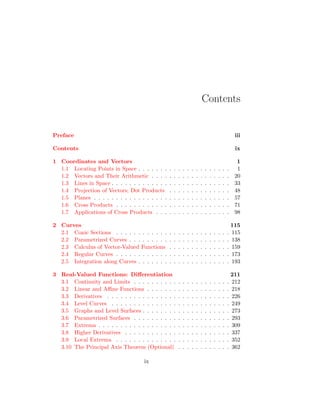
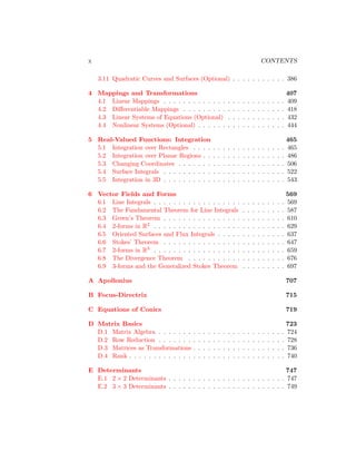
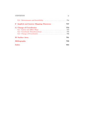


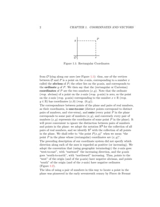
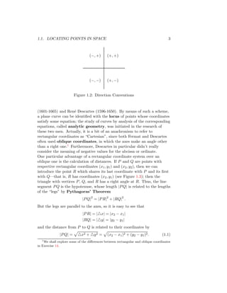
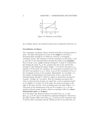
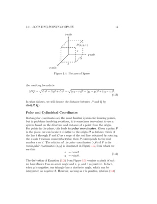
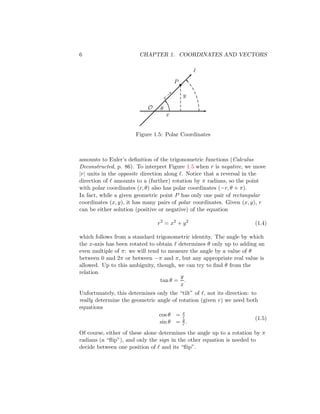
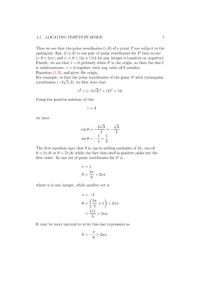
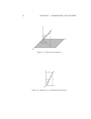
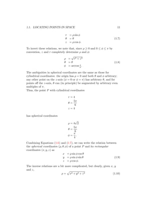
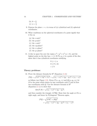
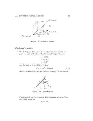
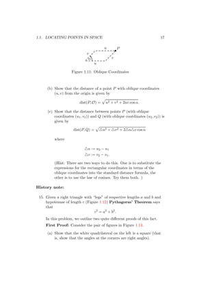
![18 CHAPTER 1. COORDINATES AND VECTORS
a
b
c
Figure 1.12: Right-angle triangle
b a
c
b
a
c
b
a
c
b
a c
a b
a
b
Figure 1.13: Pythagoras’ Theorem by Dissection
(b) Explain how the two figures prove Pythagoras’ theorem.
A variant of Figure 1.13 was used by the twelfth-century Indian
writer Bhāskara (b. 1114) to prove Pythagoras’ Theorem. His proof
consisted of a figure related to Figure 1.13 (without the shading)
together with the single word “Behold!”.
According to Eves [15, p. 158] and Maor [37, p. 63], reasoning based
on Figure 1.13 appears in one of the oldest Chinese mathematical
manuscripts, the Caho Pei Suang Chin, thought to date from the
Han dynasty in the third century B.C.
The Pythagorean Theorem appears as Proposition 47, Book I of
Euclid’s Elements with a different proof (see below). In his
translation of the Elements, Heath has an extensive commentary on
this theorem and its various proofs [29, vol. I, pp. 350-368]. In
particular, he (as well as Eves) notes that the proof above has been
suggested as possibly the kind of proof that Pythagoras himself
might have produced. Eves concurs with this judgement, but Heath
does not.
Second Proof: The proof above represents one tradition in proofs
of the Pythagorean Theorem, which Maor [37] calls “dissection
proofs.” A second approach is via the theory of proportions. Here is](https://image.slidesharecdn.com/4985394-250526101940-700539cb/85/Calculus-In-3d-Geometry-Vectors-And-Multivariate-Calculus-Draft-Nitecki-34-320.jpg)
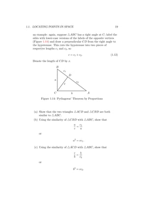
![20 CHAPTER 1. COORDINATES AND VECTORS
(d) Now combine these equations with Equation (1.12) to prove
Pythagoras’ Theorem.
The basic proportions here are those that appear in Euclid’s proof of
Proposition 47, Book I of the Elements , although he arrives at these
via different reasoning. However, in Book VI, Proposition 31 , Euclid
presents a generalization of this theorem: draw any polygon using
the hypotenuse as one side; then draw similar polygons using the legs
of the triangle; Proposition 31 asserts that the sum of the areas of
the two polygons on the legs equals that of the polygon on the
hypotenuse. Euclid’s proof of this proposition is essentially the
argument given above.
16. The Law of Cosines for an acute angle is essentially given by
Proposition 13 in Book II of Euclid’s Elements[29, vol. 1, p. 406] :
In acute-angled triangles the square on the side subtending
the acute angle is less than the squares on the sides
containing the acute angle by twice the rectangle contained
by one of the sides about the acute angle, namely that on
which the perpendicular falls, and the straight line cut off
within by the perpendicular towards the acute angle.
Translated into algebraic language (see Figure 1.15, where the acute
angle is ∠ABC) this says
A
B C
D
Figure 1.15: Euclid Book II, Proposition 13
|AC|2
= |CB|2
+ |BA|2
− |CB| |BD| .
Explain why this is the same as the Law of Cosines.
1.2 Vectors and Their Arithmetic
Many quantities occurring in physics have a magnitude and a
direction—for example, forces, velocities, and accelerations. As a](https://image.slidesharecdn.com/4985394-250526101940-700539cb/85/Calculus-In-3d-Geometry-Vectors-And-Multivariate-Calculus-Draft-Nitecki-36-320.jpg)
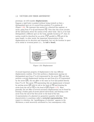
![22 CHAPTER 1. COORDINATES AND VECTORS
Figure 1.17: Combining Displacements
Aristotle (384-322 BC) [26, vol. I, p. 344], and is discussed at some length
in the Mechanics by Heron of Alexandria (ca. 75 AD) [26, vol. II, p. 348].
The vectorial nature of some physical quantities, such as velocity,
acceleration and force, was well understood and used by Isaac Newton
(1642-1727) in the Principia [41, Corollary 1, Book 1 (p. 417)]. In the late
eighteenth and early nineteenth century, Paolo Frisi (1728-1784), Leonard
Euler (1707-1783), Joseph Louis Lagrange (1736-1813), and others realized
that other physical quantities, associated with rotation of a rigid body
(torque, angular velocity, moment of a force), could also be usefully given
vectorial representations; this was developed further by Louis Poinsot
(1777-1859), Siméon Denis Poisson (1781-1840), and Jacques Binet
(1786-1856). At about the same time, various geometric quantities (e.g.,
areas of surfaces in space) were given vectorial representations by Gaetano
Giorgini (1795-1874), Simon Lhuilier (1750-1840), Jean Hachette
(1769-1834), Lazare Carnot (1753-1823)), Michel Chasles (1793-1880) and
later by Hermann Grassmann (1809-1877) and Giuseppe Peano
(1858-1932). In the early nineteenth century, vectorial representations of
complex numbers (and their extension, quaternions) were formulated by
several researchers; the term vector was coined by William Rowan
Hamilton (1805-1865) in 1853. Finally, extensive use of vectorial properties
of electromagnetic forces was made by James Clerk Maxwell (1831-1879)
and Oliver Heaviside (1850-1925) in the late nineteenth century. However,
a general theory of vectors was only formulated in the very late nineteenth](https://image.slidesharecdn.com/4985394-250526101940-700539cb/85/Calculus-In-3d-Geometry-Vectors-And-Multivariate-Calculus-Draft-Nitecki-38-320.jpg)
![1.2. VECTORS AND THEIR ARITHMETIC 23
century; the first elementary exposition was given by Edwin Bidwell
Wilson (1879-1964) in 1901 [57], based on lectures by the American
mathematical physicist Josiah Willard Gibbs (1839-1903)3 [19].
By a geometric vector in R3 (or R2) we will mean an “arrow” which can
be moved to any position, provided its direction and length are
maintained.4 We will denote vectors with a letter surmounted by an arrow,
like this: −
→
v . We define two operations on vectors. The sum of two vectors
is formed by moving −
→
w so that its “tail” coincides in position with the
“head” of −
→
v , then forming the vector −
→
v + −
→
w whose tail coincides with
that of −
→
v and whose head coincides with that of −
→
w (Figure 1.18). If
−
→
v
−
→
w
−
→
v
+
−
→
w
Figure 1.18: Sum of two vectors
instead we place −
→
w with its tail at the position previously occupied by the
tail of −
→
v and then move −
→
v so that its tail coincides with the head of −
→
w ,
we form −
→
w + −
→
v , and it is clear that these two configurations form a
parallelogram with diagonal
−
→
v + −
→
w = −
→
w + −
→
v
(Figure G.1). This is the commutative property of vector addition.
A second operation is scaling or multiplication of a vector by a
number. We naturally define
1−
→
v = −
→
v
2−
→
v = −
→
v + −
→
v
3−
→
v = −
→
v + −
→
v + −
→
v = 2−
→
v + −
→
v
and so on, and then define rational multiples by
−
→
v =
m
n
−
→
w ⇔ n−
→
v = m−
→
w;
3
I learned much of this from Sandro Caparrini [6, 7, 8]. This narrative differs from the
standard one, given by Michael Crowe [11]
4
This mobility is sometimes expressed by saying it is a free vector.](https://image.slidesharecdn.com/4985394-250526101940-700539cb/85/Calculus-In-3d-Geometry-Vectors-And-Multivariate-Calculus-Draft-Nitecki-39-320.jpg)
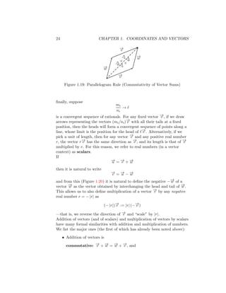
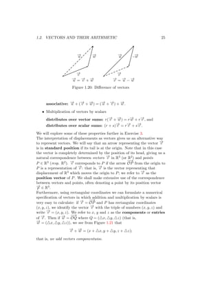
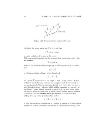
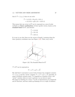
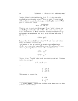
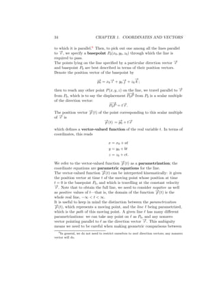

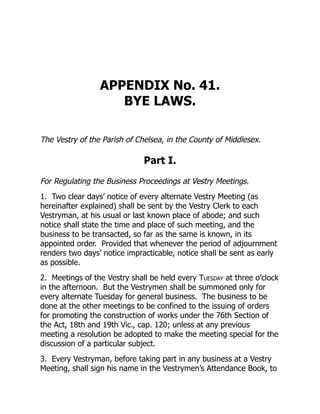
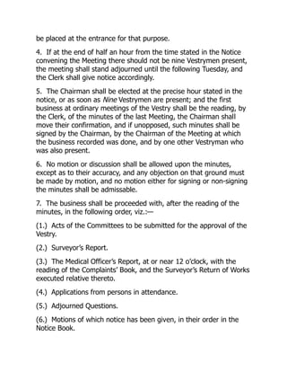
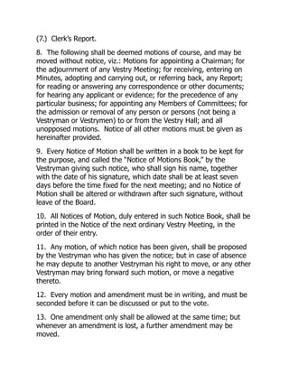
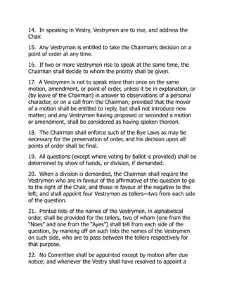
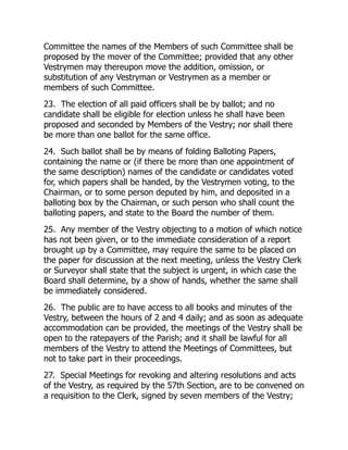
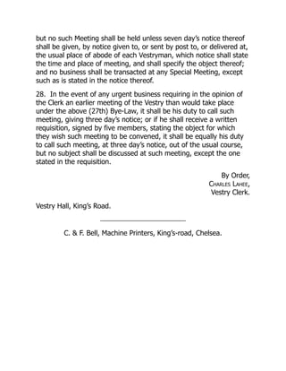
![Footnotes
[8] Commentary on the Metropolis Gas Act, 1860, by Samuel
Hughes, F.G.S., civil engineer.
[9] Many of the companies have two or three manufacturing
stations or distinct sites at which gas is made, and the wording of
the clause will probably require a testing apparatus to be erected
within 1000 yards of each separate work or manufacturing station.
[11] This title would appear be a misnomer; it is the “Sale of Gas
Act, 1859,” that is amended.
[20] The articles referred to are re-printed in the Appendix No. 20
(page 104.)
[21] See “Third Report of the Vestry of Chelsea,” page 67. The
“Charity Report” referred to in the text is simply an extract from a
book kept by the late Mr. churchwarden Fielder, and printed by order
of the vestry.
[23a] “Over against Battersea Church.”—“Old Record,” 1617.
[23b] Faulkner’s “History of Chelsea,” ed. 1829, vol. 1, p. 74.
[25] This Bill was prepared and brought in by Sir George Lewis,
Viscount Palmerston, and Lord John Russell.
[36] In the printed report Appendix 2, giving Vestry attendance etc.
is a very large, fold out table. In order to fit it better to a computer,
I’ve split it into two. Note that of the meetings, those listed to the
right Food Analysis are described as sub-committees.—DP.](https://image.slidesharecdn.com/4985394-250526101940-700539cb/85/Calculus-In-3d-Geometry-Vectors-And-Multivariate-Calculus-Draft-Nitecki-65-320.jpg)
![[37] Appointed by the Magistrates.
[116a] Report of Parish Surveyor to Vestry.
[116b] Parliamentary Return, No. 63.—page 98. 1858.
[116c] Order of Quarter Sessions, January, 1861, allowing County
Treasurer’s Account.
[116d] Mr. Laing’s Return, 1860.
[116e] Reports of Vestry: See Reports of Medical Officers.
[116f] Parliamentary Return, No. 63—page 98. 1858.
[123] The exception referred to is included in the above sum of
£5593 5s. 4d., and is an item of £21 14s. 9d., which, being for a
balance of a dinner account, is disallowed.](https://image.slidesharecdn.com/4985394-250526101940-700539cb/85/Calculus-In-3d-Geometry-Vectors-And-Multivariate-Calculus-Draft-Nitecki-66-320.jpg)