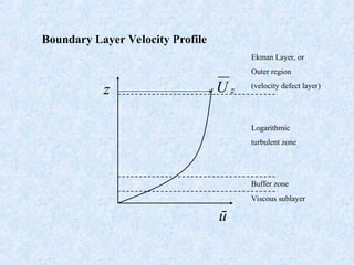
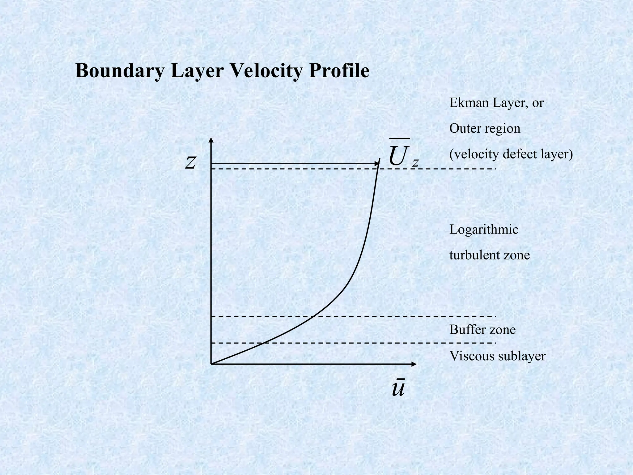
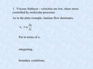
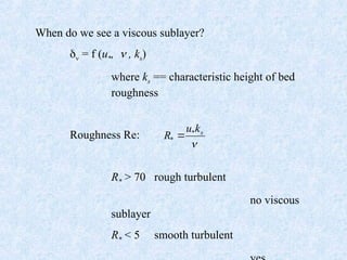
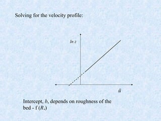
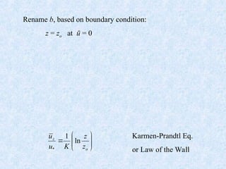
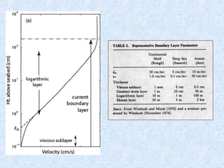
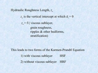
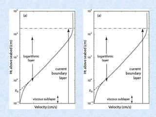
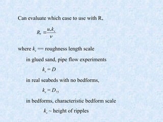
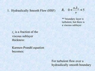
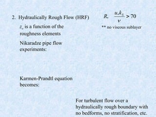
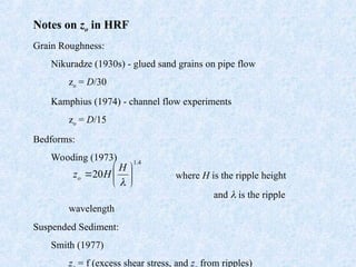
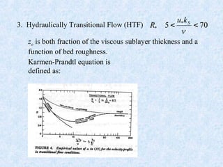
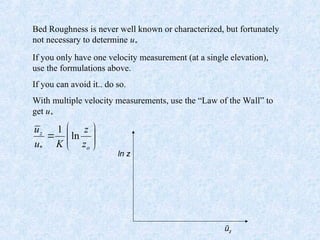
The document discusses the boundary layer velocity profile in fluid dynamics, detailing different layers such as the viscous sublayer, logarithmic layer, and turbulent zones. It explains the relationship between shear stress, roughness, and flow characteristics, referencing key theories and equations like the Karman-Prandtl equation. Additionally, it notes how roughness affects velocity profiles and provides guidance on measuring velocity in various flow conditions.

1. Boundary Layer Velocity Profile
z
ū
z
U
Viscous sublayer
Buffer zone
Logarithmic
turbulent zone
Ekman Layer, or
Outer region
(velocity defect layer)

2. But first.. a definition:
2
*
u
b 
 

3. 1. Viscous Sublayer - velocities are low, shear stress
controlled by molecular processes
As in the plate example, laminar flow dominates,
z
u
b




Put in terms of u*
integrating,
boundary conditions,

4. When do we see a viscous sublayer?
v = f (u*,  , ks)
where ks == characteristic height of bed
roughness
Roughness Re:
R* > 70 rough turbulent
no viscous
sublayer
R* < 5 smooth turbulent

s
k
u
R *
* 

5. 2. Log Layer:
Turbulent case, Az is NOT constant in z
Az is a property of the flow, not just the fluid
To describe the velocity profile we need to develop a
profile of Az.
Mixing Length formulation Prandtl (1925) which is
a qualitative argument discussed in more detail
“Boundary Layer Analysis” by Shetz, 1993
Assume that water masses act independently over a
distance, l
Within l a change in momentum causes a fluctuation
to adjacent fluid parcels.

6. At l,
Make assumption of isotropic turbulence:
|u’| ~ |v’| ~ |w’|
Therefore, |u’| ~ |w’| ~
Through the Reynolds Stress formulation,
dz
u
d
u
l
'
~
dz
u
d
l
dz
u
d
l
2
2
~
'
'








dz
u
d
l
w
u
zx
zx




Prandtl Mixing Length
Formulation

7. Von Karmen (1930) hypothesized that close to a
boundary, the turbulent exchange is related to distance
from the boundary.
l  z
l = Kz
where K is a universal turbulent momentum exchange
coefficient == von Karmen’s constant.
K has been found to be 0.41
Near the bed,
dz
u
d
Kz
u
dz
u
d
z
K
zx








*
2
2
2


in terms of u*

8. Solving for the velocity profile:
ln z
ū
Intercept, b, depends on roughness of the
bed - f (R*)

9. Rename b, based on boundary condition:
z = zo at ū = 0
Karmen-Prandtl Eq.
or Law of the Wall









o
z
z
z
K
u
u
ln
1
*

11. Hydraulic Roughness Length, zo
zo is the vertical intercept at which ūz = 0
zo = f ( viscous sublayer,
grain roughness,
ripples & other bedforms,
stratification)
This leads to two forms of the Karmen-Prandtl Equation
1) with viscous sublayer HSF
2) without viscous sublayer HRF

13. Can evaluate which case to use with R*
where ks == roughness length scale
in glued sand, pipe flow experiments
ks = D
in real seabeds with no bedforms,
ks = D75
in bedforms, characteristic bedform scale
ks ~ height of ripples

s
k
u
R *
* 

14. 1. Hydraulically Smooth Flow (HSF) 5
0 *
* 


S
k
u
R
** boundary layer is
turbulent, but there is
a viscous sublayer
zo is a fraction of the
viscous sublayer
thickness:
Karmen-Prandtl equation
becomes:
For turbulent flow over a
hydraulically smooth boundary

15. 2. Hydraulically Rough Flow (HRF) 70
*
* 

S
k
u
R
** no viscous sublayer
zo is a function of the
roughness elements
Nikaradze pipe flow
experiments:
Karmen-Prandtl equation
becomes:
For turbulent flow over a
hydraulically rough boundary with
no bedforms, no stratification, etc.

16. Notes on zo in HRF
Grain Roughness:
Nikuradze (1930s) - glued sand grains on pipe flow
zo = D/30
Kamphius (1974) - channel flow experiments
zo = D/15
Bedforms:
Wooding (1973)
where H is the ripple height
and  is the ripple
wavelength
Suspended Sediment:
Smith (1977)
z = f (excess shear stress, and z from ripples)
4
.
1
20 







H
H
zo

17. 3. Hydraulically Transitional Flow (HTF) 70
5 *
* 


S
k
u
R
zo is both fraction of the viscous sublayer thickness and a
function of bed roughness.
Karmen-Prandtl equation is
defined as:

18. Bed Roughness is never well known or characterized, but fortunately
not necessary to determine u*
If you only have one velocity measurement (at a single elevation),
use the formulations above.
If you can avoid it.. do so.
With multiple velocity measurements, use the “Law of the Wall” to
get u*









o
z
z
z
K
u
u
ln
1
*
ln z
ūz

19. To determine b (or u* ) from a velocity profile:
1. Fit line to data
2. Find slope -
3. Evaluate
)
(
ln
ln
1
2
1
2
u
u
z
z
m



m
u
K

*