Blank L, Tarquin A (2006) Solucionario Engineering Economy (6th ed).pdf

LIBROS UNIVERISTARIOS
Y SOLUCIONARIOS DE
MUCHOS DE ESTOS
LIBROS.
LOS SOLUCIONARIOS
CONTIENEN TODOS LOS
EJERCICIOS DEL LIBRO
RESUELTOS Y
EXPLICADOS DE FORMA
CLARA.
VISITANOS PARA
DESARGALOS GRATIS.
http://solucionariosdelibros.blogspot.com

By Keyser Söze
r CONOMY
Solucionario
!
Letand Blank . Anthony Tarquin

UNTVERSIDAD AUTONOMA DEL ESTADO DE MORELOS (UAEM)
FACULTAD DE CIENCIAS QUlMICAS E INGENIERIA (FCQel)
FORMULARIO DE INGENIERIA ECONOMICA
F = P(F/P,Un) F = P+Pni
A
P
Am
]
A
P = F(P/F.i.n)
P=A(P/A,
i,n)
F = A(F/A,Un)
A=F(A&l
i,n)
= G(P/G,
i,n)
F=G(F/Gl
i.n)
A=G(A/G,
iln)
I = F-P
i
porptriodo
L
m
=[hHmo0
f= >
l)M00
D P-Vs)
Pmi+f + if
X2 ~Xl J
P = A
si inj P=A(P/A.iJln)
P Si i=j P=A(P/A.iJ,n)
ING. ALFREDO PEREZ PATlto

Chapter 1 1
PROPRIETARY MATERIAL. © The McGraw-Hill Companies, Inc. All rights reserved. No part of this Manual may be
displayed, reproduced or distributed in any form or by any means, without the prior written permission of the publisher, or used
beyond the limited distribution to teachers and educators permitted by McGraw-Hill for their individual course preparation. If you are
a student using this Manual, you are using it without permission.
Chapter 1
Foundations of Engineering Economy
Solutions to Problems
1.1 Time value of money means that there is a certain worth in having money and the
worth changes as a function of time.
1.2 Morale, goodwill, friendship, convenience, aesthetics, etc.
1.3 (a) Evaluation criterion is the measure of value that is used to identify “best”.
(b) The primary evaluation criterion used in economic analysis is cost.
1.4 Nearest, tastiest, quickest, classiest, most scenic, etc
1.5 If the alternative that is actually the best one is not even recognized as an
alternative, it obviously will not be able to be selected using any economic
analysis tools.
1.6 In simple interest, the interest rate applies only to the principal, while compound
interest generates interest on the principal and all accumulated interest.
1.7 Minimum attractive rate of return is the lowest rate of return (interest rate) that
a company or individual considers to be high enough to induce them to invest
their money.
1.8 Equity financing involves the use of the corporation’s or individual’s own funds
for making investments, while debt financing involves the use of borrowed funds.
An example of equity financing is the use of a corporation’s cash or an
individual’s savings for making an investment. An example of debt financing is a
loan (secured or unsecured) or a mortgage.
1.9 Rate of return = (45/966)(100)
= 4.65%
1.10 Rate of increase = [(29 – 22)/22](100)
= 31.8%
1.11 Interest rate = (275,000/2,000,000)(100)
= 13.75%
1.12 Rate of return = (2.3/6)(100)
= 38.3%

Chapter 1 2
1.13 Profit = 8(0.28)
= $2,240,000
1.14 P + P(0.10) = 1,600,000
1.1P = 1,600,000
P = $1,454,545
1.15 Earnings = 50,000,000(0.35)
= $17,500,000
1.16 (a) Equivalent future amount = 10,000 + 10,000(0.08)
= 10,000(1 + 0.08)
= $10,800
(b) Equivalent past amount: P + 0.08P = 10,000
1.08P = 10,000
P = $9259.26
1.17 Equivalent cost now: P + 0.1P = 16,000
1.1P = 16,000
P = $14,545.45
1.18 40,000 + 40,000(i) = 50,000
i = 25%
1.19 80,000 + 80,000(i) = 100,000
i = 25%
1.20 F = 240,000 + 240,000(0.10)(3)
= $312,000
1.21 Compound amount in 5 years = 1,000,000(1 + 0.07)5
= $1,402,552
Simple amount in 5 years = 1,000,000 + 1,000,000(0.075)(5)
= $1,375,000
Compound interest is better by $27,552
1.22 Simple: 1,000,000 = 500,000 + 500,000(i)(5)
i = 20% per year simple
Compound: 1,000,000 = 500,000(1 + i)5
(1 + i)5
= 2.0000
(1 + i) = (2.0000)0.2
i = 14.87%

Chapter 1 3
1.23 Simple: 2P = P + P(0.05)(n)
P = P(0.05)(n)
n = 20 years
Compound: 2P = P(1 + 0.05)n
(1 + 0.05)n
= 2.0000
n = 14.2 years
1.24 (a) Simple: 1,300,000 = P + P(0.15)(10)
2.5P = 1,300,000
P = $520,000
(b) Compound: 1,300,000 = P(1 + 0.15)10
4.0456P = 1,300,000
P = $321,340
1.25 Plan 1: Interest paid each year = 400,000(0.10)
= $40,000
Total paid = 40,000(3) + 400,000
= $520,000
Plan 2: Total due after 3 years = 400,000(1 + 0.10)3
= $532,400
Difference paid = 532,400 – 520,000
= $12,400
1.26 (a) Simple interest total amount = 1,750,000(0.075)(5)
= $656,250
Compound interest total = total amount due after 4 years – amount borrowed
= 1,750,000(1 + 0.08)4
– 1,750,000
= 2,380856 – 1,750,000
= $630,856
(b) The company should borrow 1 year from now for a savings of $656,250 –
$630,856 = $25,394
1.27 The symbols are F = ?; P = $50,000; i = 15%; n = 3
1.28 (a) FV(i%,n,A,P) finds the future value, F
(b) IRR(first_cell:last_cell) finds the compound interest rate, i
(c) PMT(i%,n,P,F) finds the equal periodic payment, A
(d) PV(i%,n,A,F) finds the present value, P

Chapter 1 4
1.29 (a) F = ?; i = 7%; n = 10; A = $2000; P = $9000
(b) A = ?; i = 11%; n = 20; P = $14,000; F = 0
(c) P = ?; i = 8%; n = 15; A = $1000; F = $800
1.30 (a) PV = P (b) PMT = A (c) NPER = n (d) IRR = i (e) FV = F
1.31 For built-in Excel functions, a parameter that does not apply can be left blank
when it is not an interior one. For example, if there is no F involved when using
the PMT function to solve a particular problem, it can be left blank because it is
an end function. When the function involved is an interior one (like P in the PMT
function), a comma must be put in its position.
1.32 (a) Risky
(b) Safe
(c) Safe
(d) Safe
(e) Risky
1.33 (a) Equity
(b) Equity
(c) Equity
(d) Debt
(e) Debt
1.34 Highest to lowest rate of return is as follows: Credit card, bank loan to new
business, corporate bond, government bond, interest on checking account
1.35 Highest to lowest interest rate is as follows: rate of return on risky investment,
minimum attractive rate of return, cost of capital, rate of return on safe
investment, interest on savings account, interest on checking account.
1.36 WACC = (0.25)(0.18) + (0.75)(0.10) = 12%
Therefore, MARR = 12%
Select the last three projects: 12.4%, 14%, and 19%
1.37 End of period convention means that the cash flows are assumed to have occurred
at the end of the period in which they took place.
1.38 The following items are inflows: salvage value, sales revenues, cost reductions
The following items are outflows: income taxes, loan interest, rebates to dealers,
accounting services

Chapter 1 5
1.39 The cash flow diagram is:
1.40 The cash flow diagram is:
1.41 Time to double = 72/8
= 9 years
1.42 Time to double = 72/9
= 8 years
Time to quadruple = (8)(2)
= 16 years
1.43 4 = 72/i
i = 18% per year
1.44 Account must double in value five times to go from $62,500 to $2,000,000 in 20
years. Therefore, account must double every 20/5 = 4 years.
Required rate of return = 72/4
= 18% per year
FE Review Solutions
1.45 Answer is (c)
1.46 2P = P + P(0.05)(n)
n = 20
Answer is (d)
0 1 2 3
4 5 6 7 8
F= ?
$9000
$3000
$10,000
i = 10%
0 1 2 3 4 5
P = ?
$40,000
i = 15%

Chapter 1 6
1.47 Amount now = 10,000 + 10,000(0.10)
= $11,000
Answer is (c)
1.48 i = 72/9 = 8 %
Answer is (b)
1.49 Answer is (c)
1.50 Let i = compound rate of increase:
235 = 160(1 + i)5
(1 + i)5
= 235/160
(1 + i) = (1.469)0.2
(1 + i) = 1.07995
i = 7.995% = 8.0%
Answer is (c)
Extended Exercise Solution
F = ?
1. $2000
0 1 2 3 4
$500 $500 $500
$9000
F = [{[–9000(1.08) – 500] (1.08)} – 500] (1.08) + (2000–500)
= $–10,960.60
or F = –9000(F/P,8%,3) – 500(F/A,8%,3) + 2000
2. A spreadsheet uses the FV function as shown in the formula bar. F = $–10,960.61.

Chapter 1 7
3. F = [{[–9000(1.08) – 300] (1.08)} – 500] (1.08) + (2000 –1000)
= $–11,227.33
Change is 2.02%. Largest maintenance charge is in the last year and, therefore, no
compound interest is accumulated by it.
4. The fastest method is to use the spreadsheet function:
FV(12.32%,3,500,9000) + 2000
It displays the answer:
F = $–12,445.43
Microsoft EkcoI
J File Edit View Insert Format Tools Data Window Help QI Macros
D H | # | | -1 | a "|j 10
J
3
-
[i1 h - [H a B ffl
B4 =FV(B%,
3.
500,9000] +2000
El Bookl
A B C D E
1
2
4
5
($10,960.61)11
6
7
8
1
H-Solutions - Micro...
Microsoft Excel | 4:42 PM
-
SJ

Chapter 1 8
Case Study Solution
There is no definitive answer to the case study exercises. The following are
examples only.
1. The first four steps are: Define objective, information collection, alternative
definition and estimates, and criteria for decision-making.
Objective: Select the most economic alternative that also meets requirements such
as production rate, quality specifications, manufacturability for design
specifications, etc.
Information: Each alternative must have estimates for life (likely 10 years), AOC
and other costs (e.g., training), first cost, any salvage value, and the MARR. The
debt versus equity capital question must be addressed, especially if more than $5
million is needed.
Alternatives: For both A and B, some of the required data to perform an analysis
are:
P and S must be estimated.
AOC equal to about 8% of P must be verified.
Training and other cost estimates (annual, periodic, one-time) must be
finalized.
Confirm n = 10 years for life of A and B.
MARR will probably be in the 15% to 18% per year range.
Criteria: Can use either present worth or annual worth to select between A and B.
2. Consider these and others like them:
Debt capital availability and cost
Competition and size of market share required
Employee safety of plastics used in processing
3. With the addition of C, this is now a make/buy decision. Economic estimates
needed are:
 Cost of lease arrangement or unit cost, whatever is quoted.
 Amount and length of time the arrangement is available.
Some non-economic factors may be:
 Guarantee of available time as needed.
 Compatibility with current equipment and designs.
 Readiness of the company to enter the market now versus later.

Chapter 2 1
Chapter 2
Factors: How Time and Interest Affect Money
2.1 1. (F/P,8%25) = 6.8485; 2. (P/A,3%,8) = 7.0197; 3. (P/G,9%,20) = 61.7770;
4. (F/A,15%,18) = 75.8364; 5. (A/P,30%,15) = 0.30598
2.2 P = 140,000(F/P,7%,4)
=140,000(1.3108)
= $183,512
2.3 F = 200,000(F/P,10%,3)
= 200,000(1.3310)
= $266,200
2.4 P = 600,000(P/F,12%,4)
= 600,000(0.6355)
= $381,300
2.5 (a) A = 225,000(A/P,15%,4)
= 225,000(0.35027)
= $78,811
(b) Recall amount = 78,811/0.10
= $788,110 per year
2.6 F = 150,000(F/P,18%,7)
= 150,000(3.1855)
= $477,825
2.7 P = 75(P/F,18%,2)
= 75(0.7182)
= $53.865 million
2.8 P = 100,000((P/F,12%,2)
= 100,000(0.7972)
= $79,720
2.9 F = 1,700,000(F/P,18%,1)
= 1,700,000(1.18)
= $2,006,000

Chapter 2 2
2.10 P = 162,000(P/F,12%,6)
= 162,000(0.5066)
= $82,069
2.11 P = 125,000(P/F,14%,5)
= 125,000(0.5149)
= $ 64,925
2.12 P = 9000(P/F,10%,2) + 8000(P/F,10%,3) + 5000(P/F,10%,5)
= 9000(0.8264) + 8000(0.7513) + 5000(0.6209)
= $16,553
2.13 P = 1,250,000(0.10)(P/F,8%,2) + 500,000(0.10)(P/F,8%,5)
= 125,000(0.8573) + 50,000(0.6806)
= $141,193
2.14 F = 65,000(F/P,4%,5)
= 65,000(1.2167)
= $79,086
2.15 P = 75,000(P/A,20%,3)
= 75,000(2.1065)
= $157,988
2.16 A = 1.8(A/P,12%,6)
= 1.8(0.24323)
= $437,814
2.17 A = 3.4(A/P,20%,8)
= 3.4(0.26061)
= $886,074
2.18 P = (280,000-90,000)(P/A,10%,5)
= 190,000(3.7908)
= $720,252
2.19 P = 75,000(P/A,15%,5)
= 75,000(3.3522)
= $251,415
2.20 F = (458-360)(20,000)(0.90)(F/A,8%,5)
= 1,764,000(5.8666)
= $10,348,682

Chapter 2 3
2.21 P = 200,000((P/A,10%,5)
= 200,000(3.7908)
= $758,160
2.22 P = 2000(P/A,8%,35)
= 2000(11.6546)
= $23,309
2.23 A = 250,000(A/F,9%,3)
= 250,000(0.30505)
= $76,263
2.24 F = (100,000 + 125,000)(F/A,15%,3)
= 225,000(3.4725)
= $781,313
2.25 (a) 1. Interpolate between n = 32 and n = 34:
1/2 = x/0.0014
x = 0.0007
(P/F,18%,33) = 0.0050 – 0.0007
= 0.0043
2. Interpolate between n = 50 and n = 55:
4/5 = x/0.0654
x = 0.05232
(A/G,12%,54) = 8.1597 + 0.05232
= 8.2120
(b) 1. (P/F,18%,33) = 1/(1+0.18)33
= 0.0042
2. (A/G,12%,54) = {(1/0.12) – 54/[(1+0.12)54
–1}
= 8.2143
2.26 (a) 1. Interpolate between i = 18% and i = 20% at n = 20:
1/2 = x/40.06
x = 20.03
(F/A,19%,20) = 146.6280 + 20.03
=166.658
2. Interpolate between i = 25% and i = 30% at n = 15:
1/5 = x/0.5911
x = 0.11822
(P/A,26%,15) = 3.8593 – 0.11822
= 3.7411

Chapter 2 4
(b) 1. (F/A,19%,20) = [(1 + 0.19)20
– 0.19]/0.19
= 169.6811
2. (P/A,26%,15) = [(1 + 0.26)15
–1]/[0.26(1 + 0.26)15
]
= 3.7261
2.27 (a) G = $200 (b) CF8 = $1600 (c) n = 10
2.28 (a) G = $5 million (b) CF6 = $6030 million (c) n = 12
2.29 (a) G = $100 (b) CF5 = 900 – 100(5) = $400
2.30 300,000 = A + 10,000(A/G,10%,5)
300,000 = A + 10,000(1.8101)
A = $281,899
2.31 (a) CF3 = 280,000 – 2(50,000)
= $180,000
(b) A = 280,000 – 50,000(A/G,12%,5)
= 280,000 – 50,000(1.7746)
= $191,270
2.32 (a) CF3 = 4000 + 2(1000)
= $6000
(b) P = 4000(P/A,10%,5) + 1000(P/G,10%,5)
= 4000(3.7908) + 1000(6.8618)
= $22,025
2.33 P = 150,000(P/A,15%,8) + 10,000(P/G,15%,8)
= 150,000(4.4873) + 10,000(12.4807)
= $797,902
2.34 A = 14,000 + 1500(A/G,12%,5)
= 14,000 + 1500(1.7746)
= $16,662
2.35 (a) Cost = 2000/0.2
= $10,000
(b) A = 2000 + 250(A/G,18%,5)
= 2000 + 250(1.6728)
= $2418

Chapter 2 5
2.36 Convert future to present and then solve for G using P/G factor:
6000(P/F,15%,4) = 2000(P/A,15%,4) – G(P/G,15%,4)
6000(0.5718) = 2000(2.8550) – G(3.7864)
G = $601.94
2.37 50 = 6(P/A,12%,6) + G(P/G,12%,6)
50 = 6(4.1114) + G(8.9302)
G = $2,836,622
2.38 A = [4 + 0.5(A/G,16%,5)] – [1 –0.1(A/G,16%,5)
= [4 + 0.5(1.7060)] – [1 –0.1(1.7060)]
= $4,023,600
2.39 For n = 1: {1 – [(1+0.04)1
/(1+0.10)1
}]}/(0.10 –0.04) = 0.9091
For n = 2: {1 – [(1+0.04)2
/(1+0.10)2
}]}/(0.10 –0.04) = 1.7686
For n = 3: {1 – [(1+0.04)3
/(1+0.10)3
}]}/(0.10 –0.04) = 2.5812
2.40 For g = i, P = 60,000(0.1)[15/(1 + 0.04)]
= $86,538
2.41 P = 25,000{1 – [(1+0.06)3
/(1+0.15)3
}]}/(0.15 – 0.06)
= $60,247
2.42 Find P and then convert to A.
P = 5,000,000(0.01){1 – [(1+0.20)5
/(1+0.10)5
}]}/(0.10 – 0.20)
= 50,000{5.4505}
= $272,525
A = 272,525(A/P,10%,5)
= 272,525(0.26380)
= $71,892
2.43 Find P and then convert to F.
P = 2000{1 – [(1+0.10)7
/(1+0.15)7
}]}/(0.15 – 0.10)
= 2000(5.3481)
= $10,696
F = 10,696(F/P,15%,7)
= 10,696(2.6600)
= $28,452
2.44 First convert future worth to P, then use Pg equation to find A.
P = 80,000(P/F,15%,10)
= 80,000(0.2472)
= $19,776

Chapter 2 6
19,776 = A{1 – [(1+0.09)10
/(1+0.15)10
}]}/(0.15 – 0.09)
19,776 = A{6.9137}
A = $2860
2.45 Find A in year 1 and then find next value.
900,000 = A{1 – [(1+0.05)5
/(1+0.15)5
}]}/(0.15 – 0.05)
900,000 = A{3.6546)
A = $246,263 in year 1
Cost in year 2 = 246,263(1.05)
= $258,576
2.46 g = i: P = 1000[20/(1 + 0.10)]
= 1000[18.1818]
= $18,182
2.47 Find P and then convert to F.
P = 3000{1 – [(1+0.05)4
/(1+0.08)4
}]}/(0.08 –0.05)
= 3000{3.5522}
= $10,657
F = 10,657(F/P,8%,4)
= 10,657(1.3605)
= $14,498
2.48 Decrease deposit in year 4 by 5% per year for three years to get back to year 1.
First deposit = 1250/(1 + 0.05)3
= $1079.80
2.49 Simple: Total interest = (0.12)(15) = 180%
Compound: 1.8 = (1 + i)15
i = 4.0%
2.50 Profit/year = 6(3000)/0.05 = $360,000
1,200,000 = 360,000(P/A,i,10)
(P/A,i,10) = 3.3333
i = 27.3% (Excel)
2.51 2,400,000 = 760,000(P/A,i,5)
(P/A,i,5) = 3.15789
i = 17.6% (Excel)
2.52 1,000,000 = 600,000(F/P,i,5)
(F/P,i,5) = 1.6667
i = 10.8% (Excel)

Chapter 2 7
2.53 125,000 = (520,000 – 470,000)(P/A,i,4)
(P/A,i,4) = 2.5000
i = 21.9% (Excel)
2.54 400,000 = 320,000 + 50,000(A/G,i,5)
(A/G,i,5) = 1.6000
Interpolate between i = 22% and i = 24%
i = 22.6%
2.55 85,000 = 30,000(P/A,i,5) + 8,000(P/G,i,5)
Solve for i by trial and error or spreadsheet:
i = 38.9% (Excel)
2.56 500,000 = 75,000(P/A,10%,n)
(P/A,10%,n) = 6.6667
From 10% table, n is between 11 and 12 years; therefore, n = 11 years
2.57 160,000 = 30,000(P/A,12%,n)
(P/A,12%,n) = 5.3333
2.58 2,000,000 = 100,000(P/A,4%,n)
(P/A,4%,n) = 20.000
From 4% table, n is between 40 and 45 years; by spreadsheet, 42 > n > 41
Therefore, n = 41 years
2.59 1,500,000 = 3,000,000(P/F,20%,n)
(P/F,20%,n) = 0.5000
2.60 100,000 = 1,600,000(P/F,18%,n)
(P/F,18%,n) = 0.0625
2.61 10A = A(F/A,10%,n)
(F/A,10%,n) = 10.000

Chapter 2 8
2.62 1,000,000 = 10,000{1 – [(1+0.10)n
/(1+0.07)n
}]}/(0.07 – 0.10)
By trial and error, n = is between 50 and 51; therefore, n = 51 years
2.63 12,000 = 3000 + 2000(A/G,10%,n)
(A/G,10%,n) = 4.5000
FE Review Solutions
2.64 P = 61,000(P/F,6%,4)
= 61,000(0.7921)
= $48,318
Answer is (c)
2.65 160 = 235(P/F,i,5)
(P/F,i,5) =0.6809
From tables, i = 8%
Answer is (c)
2.66 23,632 = 3000{1- [(1+0.04)n
/(1+0.06)n
]}/(0.06-0.04)
[(23,632*0.02)/3000]-1 = (0.98113)n
log 0.84245 = nlog 0.98113
n = 9
Answer is (b)
2.67 109.355 = 7(P/A,i,25)
(P/A,i,25) = 15.6221
From tables, i = 4%
Answer is (a)
2.68 A = 2,800,000(A/F,6%,10)
= $212,436
Answer is (d)
2.69 A = 10,000,000((A/P,15%,7)
= $2,403,600
Answer is (a)
2.70 P = 8000(P/A,10%,10) + 500(P/G,10%,10)
= 8000(6.1446) + 500(22.8913)
= $60,602.45
Answer is (a)

Chapter 2 9
2.71 F = 50,000(F/P,18%,7)
= 50,000(3.1855)
= $159,275
Answer is (b)
2.72 P = 10,000(P/F,10%,20)
= 10,000(0.1486)
= $1486
Answer is (d)
2.73 F = 100,000(F/A,18%,5)
= 100,000(7.1542)
= $715,420
Answer is (c)
2.74 P = 100,000(P/A,10%,5) - 5000(P/G,10%,5)
= 100,000(3.7908) - 5000(6.8618)
= $344,771
Answer is (a)
2.75 F = 20,000(F/P,12%,10)
= 20,000(3.1058)
= $62,116
Answer is (a)
2.76 A = 100,000(A/P,12%,5)
= 100,000(0.27741)
= $27,741
Answer is (b)
2.77 A = 100,000(A/F,12%,3)
= 100,000(0.29635)
= $29,635
Answer is (c)
2.78 A = 10,000(F/A,12%,25)
= 10,000(133.3339)
= $1,333,339
Answer is (d)
2.79 F = 10,000(F/P,12%,5) + 10,000(F/P,12%,3) + 10,000
= 10,000(1.7623) + 10,000(1.4049) + 10,000
= $41,672
Answer is (c)

Chapter 2 10
2.80 P = 8,000(P/A,10%,5) + 900(P/G,10%,5)
= 8,000(3.7908) + 900(6.8618)
= $36,502
Answer is (d)
2.81 100,000 = 20,000(P/A,i,10)
(P/A,i,10) = 5.000
i is between 15 and 16%
Answer is (a)
2.82 60,000 = 15,000(P/A,18%,n)
(P/A,18%,n) = 4.000
n is between 7 and 8
Answer is (b)
Case Study Solution
I. Manhattan Island
Simple interest
n = 375 years from 1626 – 2001
P + I = P + nPi = 375(24)(.06) + 24
= P(1 + ni) = 24(1 + 375(.06))
= $564
Compound interest
F = P(F/P,6%,375)
= 24(3,088,157,729.0)
= $74,115,785,490, which is $74+ billion
F = ?
II. Stock-option plan after 35 years
F = ?
after 5 years
1. Years 0 1 5 35
$50/mth = 60 deposits
Age 22 27 57

Chapter 2 11
2. Value when leaving the company
F = A(F/A,1.25%,60)
= 50(88.5745)
= $4428.73
3. Value at age 57 (n = 30 years)
F = P(F/P,15%,30)
= 4428.73(66.2118)
= $293,234
4. Amount for 7 years to accumulate F = $293,234
A = F(A/F,15%,7)
= 293,234(.09036)
= $26,497 per year
5. Amount in 20’s: 5(12)50 = $3000
Amount in 50’s: 7(26,497) = $185,479

Chapter 3 1
Chapter 3
Combining Factors
3.1 P = 100,000(260)(P/A,10%,8)(P/F,10%,2)
= 26,000,000(5.3349)(0.8264)
= $114.628 million
3.2 P = 50,000(56)(P/A,8%,4)(P/F,8%,1)
= 2,800,000(3.3121)(0.9259)
= $8.587 million
3.3 P = 80(2000)(P/A,18%,3) + 100(2500)(P/A,18%,5)(P/F,18%,3)
= 160,000(2.1743) + 250,000(3.1272)(0.6086)
= $823,691
3.4 P = 100,000(P/A,15%,3) + 200,000(P/A,15%,2)(P/F,15%,3)
= 100,000(2.2832) + 200,000(1.6257)(0.6575)
= $442,100
3.5 P = 150,000 + 150,000(P/A,10%,5)
= 150,000 + 150,000(3.7908)
= $718,620
3.6 P = 3500(P/A,10%,3) + 5000(P/A,10%,7)(P/F,10%,3)
= 3500(2.4869) + 5000(4.8684)(0.7513)
= $26,992
3.7 A = [0.701(5.4)(P/A,20%,2) + 0.701(6.1)(P/A,20%,2)((P/F,20%,2)](A/P,20%,4)
= [3.7854(1.5278) + 4.2761(1.5278)(0.6944)](0.38629)
= $3.986 billion
3.8 A = 4000 + 1000(F/A,10%,4)(A/F,10%,7)
= 4000 + 1000(4.6410)(0.10541)
= $4489.21
3.9 A = 20,000(P/A,8%,4)(A/F,8%,14)
= 20,000(3.3121)(0.04130)
= $2735.79
3.10 A = 8000(A/P,10%,10) + 600
= 8000(0.16275) + 600
= $1902

Chapter 3 2
3.11 A = 20,000(F/P,8%,1)(A/P,8%,8)
= 20,000(1.08)(0.17401)
= $3758.62
3.12 A = 10,000(F/A,8%,26)(A/P,8%,30)
= 10,000(79.9544)(0.08883)
= $71,023
3.13 A = 15,000(F/A,8%,9)(A/F,8%,10)
= 15,000(12.4876)(0.06903)
= $12,930
3.14 A = 80,000(A/P,10%,5) + 80,000
= 80,000(0.26380) + 80,000
= $101,104
3.15 A = 5000(A/P,6%,5) + 1,000,000(0.15)(0.75)
= 5000(0.2374) + 112,500
= $113,687
3.16 A = [20,000(F/A,8%,11) + 8000(F/A,8%,7)](A/F,8%,10)
= [20,000(16.6455) + 8000(8.9228)]{0.06903)
= $27,908
3.17 A = 600(A/P,12%,5) + 4000(P/A,12%,4)(A/P,12%,5)
= 600(0.27741) + 4000(3.0373)(0.27741)
= $3536.76
3.18 F = 10,000(F/A,15%,21)
= 10,000(118.8101)
= $1,188,101
3.19 100,000 = A(F/A,7%,5)(F/P,7%,10)
100,000 = A(5.7507)(1.9672)
A = $8839.56
3.20 F = 9000(F/P,8%,11) + 600(F/A,8%,11) + 100(F/A,8%,5)
= 9000(2.3316) + 600(16.6455) + 100(5.8666)
= $31,558
3.21 Worth in year 5 = -9000(F/P,12%,5) + 3000(P/A,12%,9)
= -9000(1.7623) + 3000(5.3282)
= $123.90

Chapter 3 3
3.22 Amt, year 5 = 1000(F/A,12%,4)(F/P,12%,2) + 2000(P/A,12%,7)(P/F,12%,1)
= 1000(4.7793)(1.2544) + 2000(4.5638)(0.8929)
= $14,145
3.23 A = [10,000(F/P,12%,3) + 25,000](A/P,12%,7)
= [10,000(1.4049) + 25,000](0.21912)
= $8556.42
3.24 Cost of the ranch is P = 500(3000) = $1,500,000.
1,500,000 = x + 2x(P/F,8%,3)
1,500,000 = x + 2x(0.7938)
x = $579,688
3.25 Move unknown deposits to year –1, amortize using A/P, and set equal to $10,000.
x(F/A,10%,2)(F/P,10%,19)(A/P,10%,15) = 10,000
x(2.1000)(6.1159)(0.13147) = 10,000
x = $5922.34
3.26 350,000(P/F,15%,3) = 20,000(F/A,15%,5) + x
350,000(0.6575) = 20,000(6.7424) + x
x = $95,277
3.27 Move all cash flows to year 9.
0 = -800(F/A,14%,2)(F/P,14%,8) + 700(F/P,14%,7) + 700(F/P,14%,4)
–950(F/A,14%,2)(F/P,14%,1) + x – 800(P/A,14%,3)
0 = -800(2.14)2.8526) + 700(2.5023) + 700(1.6890)
–950(2.14)(1.14) + x – 800(2.3216)
x = $6124.64
3.28 Find P at t = 0 and then convert to A.
P = 5000 + 5000(P/A,12%,3) + 3000(P/A,12%,3)(P/F,12%,3)
+ 1000(P/A,12%,2)(P/F,12%,6)
= 5000 + 5000(2.4018) + 3000(2.4018)(0.7118)
+ 1000(1.6901)(0.5066)
= $22,994
A = 22,994(A/P,12%,8)
= 22,994(0.20130)
= $4628.69
3.29 F = 2500(F/A,12%,8)(F/P,12%,1) – 1000(F/A,12%,3)(F/P,12%,2)
= 2500(12.2997)(1.12) – 1000(3.3744)(1.2544)
= $30,206

Chapter 3 4
3.30 15,000 = 2000 + 2000(P/A,15%,3) + 1000(P/A,15%,3)(P/F,15%,3) + x(P/F,15%,7)
15,000 = 2000 + 2000(2.2832) + 1000(2.2832)(0.6575) + x(0.3759)
x = $18,442
3.31 Amt, year 3 = 900(F/A,16%,4) + 3000(P/A,16%,2) – 1500(P/F,16%,3)
+ 500(P/A,16%,2)(P/F,16%,3)
= 900(5.0665) + 3000(1.6052) – 1500(0.6407)
+ 500(1.6052)(0.6407)
= $8928.63
3.32 A = 5000(A/P,12%,7) + 3500 + 1500(F/A,12%,4)(A/F,12%,7)
= 5000(0.21912) + 3500 + 1500(4.7793)(0.09912)
= $5306.19
3.33 20,000 = 2000(F/A,15%,2)(F/P,15%,7) + x(F/A,15%,7) + 1000(P/A,15%,3)
20,000 = 2000(2.1500)(2.6600) + x(11.0668) + 1000(2.2832)
x = $567.35
3.34 P = [4,100,000(P/A,6%,22) – 50,000(P/G,6%,22)](P/F,6%,3)
+ 4,100,000(P/A,6%,3)
= [4,100,000(12.0416) – 50,000(98.9412](0.8396)
+ 4,100,000(2.6730)
= $48,257,271
3.35 P = [2,800,000(P/A,12%,7) + 100,000(P/G,12%,7) + 2,800,000](P/F,12%,1)
= [2,800,000(4.5638) + 100,000(11.6443) + 2,800,000](0.8929)
= $14,949,887
3.36 P for maintenance = [11,500(F/A,10%,2) + 11,500(P/A,10%,8)
+ 1000(P/G,10%,8)](P/F,10%,2)
= [11,500(2.10) + 11,500(5.3349) + 1000(16.0287)](0.8264)
= $83,904
P for accidents = 250,000(P/A,10%,10)
= 250,000(6.1446)
= $1,536,150
Total savings = 83,904 + 1,536,150
= $1,620,054
Build overpass
3.37 Find P at t = 0, then convert to A.
P = [22,000(P/A,12%,4) + 1000(P/G,12%,4) + 22,000](P/F,12%,1)
= [22,000(3.0373) + 1000(4.1273) + 22,000](0.8929)
= $82,993

Chapter 3 5
A = 82,993(A/P,12%,5)
= 82,993(0.27741)
= $23,023
3.38 First find P and then convert to F.
P = -10,000 + [4000 + 3000(P/A,10%,6) + 1000(P/G,10%,6)
– 7000(P/F,10%,4)](P/F,10%,1)
= -10,000 + [4000 + 3000(4.3553) + 1000(9.6842)
– 7000(0.6830)](0.9091)
= $9972
F = 9972(F/P,10%,7)
= 9972(1.9487)
= $19,432
3.39 Find P in year 0 and then convert to A.
P = 4000 + 4000(P/A,15%,3) – 1000(P/G,15%,3) + [(6000(P/A,15%,4)
+2000(P/G,15%,4)](P/F,15%,3)
= 4000 + 4000(2.2832) – 1000(2.0712) + [(6000(2.8550)
+2000(3.7864)](0.6575)
= $27,303.69
A = 27,303.69(A/P,15%,7)
= 27,303.69(0.24036)
= $6563
3.40 40,000 = x(P/A,10%,2) + (x + 2000)(P/A,10%,3)(P/F,10%,2)
40,000 = x(1.7355) + (x + 2000)(2.4869)(0.8264)
3.79067x = 35,889.65
x = $9467.89 (size of first two payments)
3.41 11,000 = 200 + 300(P/A,12%,9) + 100(P/G,12%,9) – 500(P/F,12%,3)
+ x(P/F,12%,3)
11,000 = 200 + 300(5.3282) + 100(17.3563) – 500(0.7118) + x(0.7118)
x = $10,989
3.42 (a) In billions
P in yr 1 = -13(2.73) + 5.3{[1 – (1 + 0.09)10
/ (1 + 0.15)10
]/(0.15 – 0.09)}
= -35.49 + 5.3(6.914)
= $1.1542 billion
P in yr 0 = 1.1542(P/F,15%,1)
= 1.1542(0.8696)
= $1.004 billion

Chapter 3 6
3.43 Find P in year –1; then find A in years 0-5.
Pg in yr 2 = (5)(4000){[1 - (1 + 0.08)18
/(1 + 0.10)18
]/(0.10 - 0.08)}
= 20,000(14.0640)
= $281,280
P in yr –1 = 281,280(P/F,10%,3) + 20,000(P/A,10%,3)
= 281,280(0.7513) + 20,000(2.4869)
= $261,064
A = 261,064(A/P,10%,6)
= 261,064(0.22961)
= $59,943
3.44 Find P in year –1 and then move forward 1 year
P-1= 20,000{[1 – (1 + 0.05)11
/(1 + 0.14)11
]/(0.14 – 0.05)}.
= 20,000(6.6145)
= $132,290
P = 132,290(F/P,14%,1)
= 132,290(1.14)
= $150,811
3.45 P = 29,000 + 13,000(P/A,10%,3) + 13,000[7/(1 + 0.10)](P/F,10%,3)
= 29,000 + 13,000(2.4869) + 82,727(0.7513)
= $123,483
3.46 Find P in year –1 and then move to year 0.
P (yr –1) = 15,000{[1 – (1 + 0.10)5
/(1 + 0.16)5
]/(0.16 – 0.10)}
= 15,000(3.8869)
= $58,304
P = 58,304(F/P,16%,1)
= 58,304(1.16)
= $67,632
3.47 Find P in year –1 and then move to year 5.
P (yr –1) = 210,000[6/(1 + 0.08)]
= 210,000(0.92593)
= $1,166,667
F = 1,166,667(F/P,8%,6)
= 1,166,667(1.5869)
= $1,851,383

Chapter 3 7
3.48 P = [2000(P/A,12%,6) – 200(P/G,12%,6)](F/P,12%,1)
= [2000(4.1114) – 200(8.9302](1.12)
= $7209.17
3.49 P = 5000 + 1000(P/A,12%,4) + [1000(P/A,12%,7) – 100(P/G,12%,7)](P/F,12%,4)
= 5000 + 1000(3.0373) + [1000(4.5638) – 100(11.6443)](0.6355)
= $10,198
3.50 Find P in year 0 and then convert to A.
P = 2000 + 2000(P/A,10%,4) + [2500(P/A,10%,6) – 100(P/G,10%,6)](P/F,10%,4)
= 2000 + 2000(3.1699) + [2500(4.3553) – 100(9.6842)](0.6830)
= $15,115
A = 15,115(A/P,10%,10)
= 15,115(0.16275)
= $2459.97
3.51 20,000 = 5000 + 4500(P/A,8%,n) – 500(P/G,8%,n)
Solve for n by trial and error:
Try n = 5: $15,000 > $14,281
Try n = 6: $15,000 < $15,541
By interpolation, n = 5.6 years
3.52 P = 2000 + 1800(P/A,15%,5) – 200(P/G,15%,5)
= 2000 + 1800(3.3522) – 200(5.7751)
= $6878.94
3.53 F = [5000(P/A,10%,6) – 200(P/G,10%,6)](F/P,10%,6)
= [5000(4.3553) – 200(9.6842)](1.7716)
= $35,148
FE Review Solutions
3.54 x = 4000(P/A,10%,5)(P/F,10%,1)
= 4000(3.7908)(0.9091)
= $13,785
Answer is (d)
3.55 P = 7 + 7(P/A,4%,25)
= $116.3547 million
Answer is (c)
3.56 Answer is (d)

Chapter 3 8
3.57 Size of first deposit = 1250/(1 + 0.05)3
= $1079.80
Answer is (d)
3.58 Balance = 10,000(F/P,10%,2) – 3000(F/A,10%,2)
= 10,000(1.21) – 3000(2.10)
= $5800
Answer is (b)
3.59 1000 = A(F/A,10%,5)(A/P,10%,20)
1000 = A(6.1051)(0.11746)
A = $1394.50
Answer is (a)
3.60 First find P and then convert to A.
P = 1000(P/A,10%,5) + 2000(P/A,10%,5)(P/F,10%,5)
= 1000(3.7908) + 2000(3.7908)(0.6209)
= $8498.22
A = 8498.22(A/P,10%,10)
= 8498.22(0.16275)
= $1383.08
Answer is (c)
3.61 100,000 = A(F/A,10%,4)(F/P,10%,1)
100,000 = A(4.6410)(1.10)
A = $19,588
Answer is (a)
3.62 F = [1000 + 1500(P/A,10%,10) + 500(P/G,10%,10](F/P,10%,10)
= [1000 + 1500(6.1446) + 500(22.8913](2.5937)
= $56,186
Answer is (d)
3.63 F = 5000(F/P,10%,10) + 7000(F/P,10%,8) + 2000(F/A,10%,5)
= 5000(2.5937) + 7000(2.1438) + 2000(6.1051)
= $40,185
Answer is (b)

Chapter 3 9
Solution by Hand
Cash flows for purchases at g = –25% start in year 0 at $4 million. Cash flows for parks
development at G = $100,000 start in year 4 at $550,000. All cash flow signs in the
solution are +.
Cash flow________
Year Land Parks
0 $4,000,000
1 3,000,000
2 2,250,000
3 1,678,000
4 1,265.625 $550,000
5 949,219 650,000
6 750,000
1. Find P for all project funds (in $ million)
P = 4 + 3(P/F,7%,1) + … + 0.750(P/F,7%,6)
= 13.1716 ($13,171,600)
Amount to raise in years 1 and 2:
A = (13.1716 – 3.0)(A/P,7%,2)
= (10.1716)(0.55309)
= 5.6258 ($5,625,800 per year)
2. Find remaining project fund needs in year 3, then find the A for the next 3 years
(years 4, 5, and 6):
F3 = (13.1716 – 3.0)(F/P,7%,3)
= (10.1716)(1.2250)
= 12.46019
A = 12.46019(A/P,7%,3)
= 12.46019(0.38105)
= 4.748 ($4,748,000 per year)

Chapter 3 10
Solution by computer
E Microsoft Excel
File Edit View Insert Format lools Data Window Help QI Macros
X
B I , A .
J
H22
E l C3 ext exer soln
A B C D
1
2
3
Chapter 3 - extended exercise solution
Interest rate = 7%
.
and purchase multiplier = 0,75
E F
_
4|Amount from bonds now = If
5 Parks csh flow gradient, G = If
6
_
7
_
"
SlYear
3,
000,
000
100.
000
Cash flows
0 %
1 It
Land purchases Parks development
2 $
3 $
4 $
J3_
iL
11
12
_
il
H
17 P for purchases
18
_
P values $ 11,788,797
ii.
20
5 $
6 $
4,
000,000 $
3,
000,000 $
2,
250,000 $
1,
687,500 $
1,
265,625 $
949,219 If
-
$
550.
000
650.
000
750.
000
I
P for parks Total present worth
1,
382.
790 $ 13,
171.
587
dy
1) To raise; Yrs. 1 and 2 : $5,625,821
2) To raise: Yrs, 4. 5 and 6= $4.748.145
AutoShapes - O HMUIi <2» - . A >
"
i r NUM
"
i r

Chapter 4 1
Chapter 4
Nominal and Effective Interest Rates
4.1 (a) monthly (b) quarterly (c) semiannually
4.2 (a) quarterly (b) monthly (c) weekly
4.3 (a) 12 (b) 4 (c) 2
4.4 (a) 1 (b) 4 (c) 12
4.5 (a) r/semi = 0.5*2 = 1% (b) 2% (c) 4%
4.6 (a) i = 0.12/6 = 2% per two months; r/4 months = 0.02*2 = 4%
(b) r/6 months = 0.02*3 = 6%
(c) r/2 yrs = 0.02*12 = 24%
4.7 (a) 5% (b) 20%
4.8 (a) effective (b) effective (c) nominal (d) effective (e) nominal
4.9 i/6months = 0.14/2 = 7%
4.10 i = (1 + 0.04)4
– 1
= 16.99%
4.11 0.16 = (1 + r/2)2
–1
r = 15.41%
4.12 Interest rate is stated as effective. Therefore, i = 18%
4.13 0.1881 = (1 + 0.18/m)m
– 1
Solve for m by trial and gives m = 2
4.14 i = (1 + 0.01)2
–1
i = 2.01%

Chapter 4 2
4.15 i = 0.12/12 = 1% per month
Nominal per 6 months = 0.01(6) = 6%
Effective per 6 months = (1 + 0.06/6)6
– 1
= 6.15%
4.16 (a) i/week = 0.068/26 = 0.262%
(b) effective
4.17 PP = weekly; CP = quarterly
4.18 PP = daily; CP = quarterly
4.19 From 2% table at n =12, F/P = 1.2682
4.20 Interest rate is effective
From 6% table at n = 5, P/G = 7.9345
4.21 P = 85(P/F,2%,12) = 85(0.7885)
= $67.02 million
4.22 F = 2.7(F/P,3%,60)
= 2.7(5.8916)
= $15.91 billion
4.23 P = 5000(P/F,4%,16)
= 5000(0.5339)
= $2669.50
4.24 P = 1.2(P/F,5%,1) (in $million)
= 1.2(0.9524)
= $1,142,880
4.25 P = 1.3(P/A,1%,28)(P/F,1%,2) (in $million)
= 1.3(24.3164)(0.9803)
= $30,988,577
4.26 F = 3.9(F/P,0.5%,120) (in $billion)
= 3.9(1.8194)
= $7,095,660,000
4.27 P = 3000(250 – 150)(P/A,4%,8) (in $million)
= 3000(100)(6.7327)
= $2,019,810

Chapter 4 3
4.28 F = 50(20,000,000)(F/P,1.5%,9)
= 1,000,000,000(1.1434)
= $1.1434 billion
4.29 A = 3.5(A/P,5%,12) (in $million)
= 3.5(0.11283)
= $394,905
4.30 F = 10,000(F/P,4%,4) + 25,000(F/P,4%,2) + 30,000(F/P,4%,1)
= 10,000(1.1699) + 25,000(1.0816) + 30,000(1.04)
= $69,939
4.31 i/wk = 0.25%
P = 2.99(P/A,0.25%,40)
= 2.99(38.0199)
= $113.68
4.32 i/6 mths = (1 + 0.03)2
– 1
A = 20,000(A/P,6.09%,4)
= 20,000 {[0.0609(1 + 0.0609)4
]/[(1 + 0.0609)4
-1]}
= 20,000(0.28919)
= $5784
4.33 F = 100,000(F/A,0.25%,8)(F/P,0.25%,3)
= 100,000(8.0704)(1.0075)
= $813,093
Subsidy = 813,093 – 800,000 = $13,093
4.34 P = (14.99 – 6.99)(P/A,1%,24)
= 8(21.2434)
= $169.95
4.35 First find P, then convert to A
P = 150,000{1 – [(1+0.20)10
/(1+0.07)10
}]}/(0.07 – 0.20)
= 150,000(16.5197)
= $2,477,955
A = 2,477,955(A/P,7%,10)
= 2,477,955(0.14238)
= $352,811

Chapter 4 4
4.36 P = 80(P/A,3%,12) + 2(P/G,3%,12)
P = 80(9.9540) + 2(51.2482)
= $898.82
4.37 2,000,000 = A(P/A,3%,8) + 50,000(P/G,3%,8)
2,000,000 = A(7.0197) + 50,000(23.4806)
A = $117,665
4.38 P = 1000 + 2000(P/A,1.5%,12) + 3000(P/A,1.5%,16)(P/F,1.5%,12)
= 1000 + 2000(10.9075) + 3000(14.1313)(0.8364)
= $58,273
4.39 First find P in quarter –1 and then use A/P to get A in quarters 0-8.
P-1 = 1000(P/F,4%,2) + 2000(P/A,4%,2)(P/F,4%,2) + 3000(P/A,4%,4)(P/F,4%,5)
= 1000(0.9246) + 2000(1.8861)(0.9246) + 3000(3.6299)(0.8219)
= $13,363
A = 13,363(A/P,4%,9)
= 13,363(0.13449)
= $1797.19
4.40 Move deposits to end of compounding periods and then find F.
F = 1800(F/A,3%,30)
= 1800(47.5754)
= $85,636
4.41 Move withdrawals to beginning of periods and then find F.
F = (10,000 – 1000)(F/P,4%,6) – 1000(F/P,4%,5) – 1000(F/P,4%,3)
= 9000(1.2653) – 1000(1.2167) – 1000(1.1249)
= $9046
4.42 Move withdrawals to beginning of periods and deposits to end; then find F.
F = 1600(F/P,4%,5) +1400(F/P,4%,4) – 2600(F/P,4%,3) + 1000(F/P,4%,2)
-1000(F/P,4%,1)
= 1600(1.2167) + 1400(1.1699) – 2600(1.1249) + 1000(1.0816) –1000(1.04)
= $701.44
4.43 Move monthly costs to end of quarter and then find F.
Monthly costs = 495(6)(2) = $5940
End of quarter costs = 5940(3) = $17,820
F = 17,820(F/A,1.5%,4)
= 17,820(4.0909)
= $72,900

Chapter 4 5
4.44 i = e0.13
– 1
= 13.88%
4.45 i = e0.12
– 1
= 12.75%
4.46 0.127 = er
– 1
r/yr = 11.96%
r /quarter = 2.99%
4.47 15% per year = 15/12 = 1.25% per month
i = e0.0125
– 1 = 1.26% per month
F = 100,000(F/A,1.26%,24)
= 100,000{[1 + 0.0126)24
–1]/0.0126}
= 100,000(27.8213)
= $2,782,130
4.48 18% per year = 18/12 = 1.50% per month
i = e0.015
– 1 = 1.51% per month
P = 6000(P/A,1.51%,60)
= 6000{[(1 + 0.0151)60
– 1]/[0.0151(1 + 0.0151)60
]}
= 6000(39.2792)
= $235,675
4.49 i = e0.02
– 1 = 2.02% per month
A = 50(A/P,2.02%,36)
= 50{[0.0202(1 + 0.0202)36
]/[(1 + 0.0202)36
– 1]}
= 50(0.03936)
= $1,968,000
4.50 i = e0.06
– 1 = 6.18% per year
P = 85,000(P/F,6.18%,4)
= 85,000[1/(1 + 0.0618)4
= 85,000(0.78674)
= $66,873
4.51 i = e0.015
– 1 = 1.51% per month
2P = P(1 + 0.0151)n
2.000 = (1.0151) n
Take log of both sides and solve for n
n = 46.2 months

Chapter 4 6
4.52 Set up F/P equation in months.
3P = P(1 + i)60
3.000 = (1 + i)60
1.01848 = 1 + i
i = 1.85% per month (effective)
4.53 P = 150,000(P/F,12%,2)(P/F,10%,3)
= 150,000(0.7972)(0.7513)
= $89,840
4.54 F = 50,000(F/P,10%,4)(F/P,1%,48)
= 50,000(1.4641)(1.6122)
= $118,021
4.55 (a) First move cash flow in years 0-4 to year 4 at i = 12%.
F = 5000(F/P,12%,4) + 6000(F/A,12%,4)
= 5000(1.5735) + 6000(4.7793)
= $36,543
Now move the total to year 5 at i = 20%.
F = 36,543(F/P,20%,1) + 9000
= 36,543(1.20) + 9000
= $52,852
(b) Substitute A values for annual cash flows, including year 5 with the factor
(F/P,20%,0) = 1.00
52,852 = A{[(F/P,12%,4) + (F/A,12%,4)](F/P,20%,1) + (F/P,20%,0)}
= A{[(1.5735) + (4.7793)](1.20) + 1.00}
= A(8.62336)
A = $6129 per year for years 0 through 5 ( a total of 6 A values).
4.56 First find P.
P = 5000(P/A,10%,3) + 7000(P/A,12%,2)(P/F,10%3)
= 5000(2.4869) + 7000(1.6901)(0.7513)
= 12,434.50 + 8888.40
= $21,323

Chapter 4 7
Now substitute A values for cash flows.
21,323 = A(P/A,10%,3) + A(P/A,12%,2)(P/F,10%3)
= A(2.4869) + A(1.6901)(0.7513)
= A(3.7567)
A = $5676
FE Review Solutions
4.57 Answer is (b)
4.58 Answer is (d)
4.59 i/yr = (1 + 0.01)12
–1 = 0.1268 = 12.68%
Answer is (d)
4.60 i/quarter = e0.045
–1 = 0.0460 = 4.60%
Answer is (c)
4.61 Answer is (d)
4.62 Answer is (a)
4.63 Find annual rate per year for each condition.
i/yr = 22% simple
i/yr = (1 + 0.21/4)4
–1 = 0.2271 = 22.7 %
i/yr = (1 + 0.21/12)12
–1 = 0.2314 = 23.14 %
i/yr = (1 + 0.22/2)2
–1 = 0.2321 = 23.21 %
Answer is (a)
4.64 i/semi-annual = e0.02
–1 = 0.0202 = 2.02%
Answer is (b)
4.65 Answer is (c)
4.66 P = 30(P/A,0.5%,60)
= $1552
Answer is (b)

Chapter 4 8
4.67 P = 7 + 7(P/A,4%,25)
= $116.3547 million
Answer is (c)
4.68 Answer is (a)
4.69 Answer is (d)
4.70 PP>CP; must use i over PP of 1 year. Therefore, n = 7
Answer is (a)
4.71 P = 1,000,000 + 1,050,000{[1- [(1 + 0.05)12
/( 1 + 0.01)12
]}/(0.01-0.05)
= $16,585,447
Answer is (b)
4.72 Answer is (d)
4.73 Deposit in year 1 = 1250/(1 + 0.05)3
= $1079.80
Answer is (d)
4.74 A = 40,000(A/F,5%,8)
= 40,000(0.10472)
= $4188.80
Answer is (c)
4.75 A = 800,000(A/P,3%,12)
= 800,000(0.10046)
= $80,368
Answer is (c)
Case Study Solution
1. Plan C:15-Year Rate - The calculations for this plan are the same as those for plan A,
except that i = 9 ½% per year and n = 180 periods instead of 360. However, for a 5%
down payment, the P&I is now $1488.04 which will yield a total payment of
$1788.04. This is greater than the $1600 maximum payment available. Therefore, the
down payment will have to be increased to $25,500, making the loan amount
$124,500. This will make the P&I amount $1300.06 for a total monthly payment of
$1600.06.

Chapter 4 9
The amount of money required up front is now $28,245 (the origination fee has also
changed). The plan C values for F1C, F2C, and F3C are shown below.
F1C = (40,000 – 28,245)(F/P,0.25%,120)
= $15,861.65
F2C = 0
F3C = 170,000 – [124,500(F/P,9.5%/12,120)
– 1300.06(F/A,9.5%/12,120)
= $108,097.93
FC = F1C + F2C + F3C
= $123,959.58
The future worth of Plan C is considerably higher than either Plan A ($87,233) or
Plan B ($91,674). Therefore, Plan C with a 15-year fixed rate is the preferred
financing method.
2. Plan A
Loan amount = $142,500
Balance after 10 years = $129,582.48
Equity = 142,500 – 129,582.48 = $12,917.52
Total payment made = 1250.56(120) = $150,067.20
Interest paid = 150,067.20 – 12,917.52 = $137,149.68
3. Amount paid through first 3 yrs = 1146.58 (36) = $41,276.88
Principal reduction through first 3 yrs = 142,500 – 139,297.08 = $3,202.92
Interest paid first 3 yrs = 41,276.88 – 3202.92 = $38,073.96
Amount paid year 4 = 1195.67(12) = 14,348.04
Principal reduction year 4 = 139,297.08 – 138,132.42 = 1164.66
Interest paid year 4 = 14,348.04 – 1164.66 = 13,183.38
Total interest paid in 4 years = 38,073.96 + 13,183.38 = $51,257.34
4. Let DP = down payment
Fixed fees = 300 + 200 + 200 + 350 + 150 + 300 = $1500
Available for DP = 40,000 – 1500 – (loan amount)(0.01)
where loan amount = 150,000 – DP

Chapter 4 10
DP = 40,000 – 1500 - (150,000 – DP)(0.01)
= 40,000 – 1500 – 1500 + 0.01DP
0.99DP = 37,000
DP = $37,373.73
check: origination fee = (150,000 – 37,373.73)(0.01) = 1126.26
available DP = 40,000 – 1500 – 1126.26 = $37,373.73
5. Amount financed = $142,500 Increase from
one interest rate
Monthly P&I @ 10% = $1,250.56 to the other
Monthly P&I @ 11% = 142,500(A/P,11%/12, 60) -----
A = (142,500) (0.009167)(1 + 0.009167)360
= $1357.06 106.50
(1 + 0.009167)360
– 1
Monthly P&I @ 12% = $1465.77 108.71
Monthly P&I @ 13% = $1576.33 110.56
Monthly P&I @ 14% = $1688.44 112.11
Increase varies: 10% to 11% = $106.50
11% to 12% = 108.71
12% to 13% = 110.56
13% to 14% = 112.11
6. In buying down interest, you must give lender money now instead of money later.
Therefore, to go from 10% to 9%, lender must recover the additional 1% now.
103.95/month
P&I @ 10% = 1250.54
P&I @ 9% = 1146.59 …
Difference = $103.95/month 1 2 3 . . . . . . 360
month
P = 103.95(P/A,10%/12,360) P
= 103.95(113.9508)
= $11,845.19

Chapter 5 1
Chapter 5
Present Worth Analysis
5.1 A service alternative is one that has only costs (no revenues).
5.2 (a) For independent projects, select all that have PW ≥ 0; (b) For mutually
exclusive projects, select the one that has the highest numerical value.
5.3 (a) Service; (b) Revenue; (c) Revenue; (d) Service; (e) Revenue; (f) Service
5.4 (a) Total possible = 25
= 32
(b) Because of restrictions, cannot have any combinations of 3,4, or 5. Only 12 are
acceptable: DN, 1, 2, 3, 4, 5, 1&3, 1&4, 1&5, 2&3, 2&4, and 2&5.
5.5 Equal service means that the alternatives end at the same time.
5.6 Equal service can be satisfied by using a specified planning period or by using the
least common multiple of the lives of the alternatives.
5.7 Capitalized cost represents the present worth of service for an infinite time. Real
world examples that might be analyzed using CC would be Yellowstone National
Park, Golden Gate Bridge, Hoover Dam, etc.
5.8 PWold = -1200(3.50)(P/A,15%,5)
= -4200(3.3522)
= $-14,079
PWnew = -14,000 – 1200(1.20)(P/A,15%,5)
= -14,000 – 1440(3.3522)
= $-18,827
Keep old brackets
5.9 PWA = -80,000 – 30,000(P/A,12%,3) + 15,000(P/F,12%,3)
= -80,000 – 30,000(2.4018) + 15,000(0.7118)
= $-141,377

Chapter 5 2
PWB = -120,000 – 8,000(P/A,12%,3) + 40,000(P/F,12%,3)
= -120,000 – 8,000(2.4018) + 40,000(0.7118)
= $-110,742
Select Method B
5.10 Bottled water: Cost/mo = -(2)(0.40)(30) = $24.00
PW = -24.00(P/A,0.5%,12)
= -24.00(11.6189)
= $-278.85
Municipal water: Cost/mo = -5(30)(2.10)/1000 = $0.315
PW = -0.315(P/A,0.5%,12)
= -0.315(11.6189)
= $-3.66
5.11 PWsingle = -4000 - 4000(P/A,12%,4)
= -4000 - 4000(3.0373)
= $-16,149
PWsite = $-15,000
Buy the site license
5.12 PWvariable = -250,000 – 231,000(P/A,15%,6) – 140,000(P/F,15%,4)
+ 50,000(P/F,15%,6)
= -250,000 – 231,000(3.7845) – 140,000(0.5718) + 50,000(0.4323)
= $-1,182,656
PWdual = -224,000 –235,000(P/A,15%,6) –26,000(P/F,15%,3)
+ 10,000(P/F,15%,6)
= -224,000 –235,000(3.7845) –26,000(0.6575) + 10,000(0.4323)
= $-1,126,130
Select dual speed machine
5.13 PWJX = -205,000 – 29,000(P/A,10%,4) – 203,000(P/F,10%,2)
+ 2000(P/F,10%,4)
= -205,000 – 29,000(3.1699) – 203,000(0.8264) + 2000(0.6830)
= $-463,320
PWKZ = -235,000 – 27,000(P/A,10%,4) + 20,000(P/F,10%,4)
= -235,000 – 27,000(3.1699) + 20,000(0.6830)
= $-306,927
Select material KZ

Chapter 5 3
5.14 PWK = -160,000 – 7000(P/A,2%,16) –120,000(P/F,2%,8) + 40,000(P/F,2%,16)
= -160,000 – 7000(13.5777) –120,000(0.8535) + 40,000(0.7284)
= $-328,328
PWL = -210,000 – 5000(P/A,2%,16) + 26,000(P/F,2%,16)
= -210,000 – 5000(13.5777) + 26,000(0.7284)
= $-258,950
Select process L
5.15 PWplastic = -75,000 - 27,000(P/A,10%,6) - 75,000(P/F,10%,2)
- 75,000(P/F,10%,4)
= -75,000 - 27,000(4.3553) - 75,000(0.8264) - 75,000(0.6830)
= $-305,798
PWaluminum = -125,000 – 12,000(P/A,10%,6) – 95,000(P/F,10%,3)
+ 30,000(P/F,10%,6)
= -125,000 – 12,000(4.3553) – 95,000(0.7513) + 30,000(0.5645)
= $-231,702
Use aluminum case
5.16 i/year = (1 + 0.03)2
– 1 = 6.09%
PWA = -1,000,000 - 1,000,000(P/A,6.09%,5)
= -1,000,000 - 1,000,000(4.2021) (by equation)
= $-5,202,100
PWB = -600,000 – 600,000(P/A,3%,11)
= -600,000 – 600,000(9.2526)
= $-6,151,560
PWC = -1,500,000 – 500,000(P/F,3%,4) – 1,500,000(P/F,3%,6)
- 500,000(P/F,3%,10)
= -1,500,000 – 500,000(0.8885) – 1,500,000(0.8375) – 500,000(0.7441)
= $-3,572,550
Select plan C
5.17 FWsolar = -12,600(F/P,10%,4) – 1400(F/A,10%,4)
= -12,600(1.4641) – 1400(4.6410)
= $-24,945
FWline = -11,000(F/P,10%,4) – 800(F/P,10%,4)
= -11,000(1.4641) – 800(4.6410)
= $-19,818
Install power line

Chapter 5 4
5.18 FW20% = -100(F/P,10%,15) – 80(F/A,10%,15)
= -100(4.1772) – 80(31.7725)
= $-2959.52
FW35% = -240(F/P,10%,15) – 65(F/A,10%,15)
= -240(4.1772) – 65(31.7725)
= $-3067.74
20% standard is slightly more economical
5.19 FWpurchase = -150,000(F/P,15%,6) + 12,000(F/A,15%,6) + 65,000
= -150,000(2.3131) + 12,000(8.7537) + 65,000
= $-176,921
FWlease = -30,000(F/A,15%,6)(F/P,15%,1)
= - 30,000(8.7537)(1.15)
= $-302,003
Purchase the clamshell
5.20 FWHSS = -3500(F/P,1%,6) –2000(F/A,1%,6) – 3500(F/P,1%,3)
= -3500(1.0615) –2000(6.1520) – 3500(1.0303)
= $-19,625
FWgold = -6500(F/P,1%,6) –1500(F/A,1%,6)
= -6500(1.0615) –1500(6.1520)
= $-16,128
FWtitanium = -7000(F/P,1%,6) –1200(F/A,1%,6)
= -7000(1.0615) –1200(6.1520)
= $-14,813
Use titanium nitride bits
5.21 FWA = -300,000(F/P,12%,10) – 900,000(F/A,12%,10)
= -300,000(3.1058) – 900,000(17.5487)
= $-16,725,570
FWB = -1,200,000(F/P,12%,10) – 200,000(F/A,12%,10)
– 150,000(F/A,12%,10)
= -1,200,000(3.1058) – 200,000(17.5487) – 150,000(17.5487)
= $-9,869,005
Select Plan B

Chapter 5 5
5.22 CC = -400,000 – 400,000(A/F,6%,2)/0.06
= -400,000 – 400,000(0.48544)/0.06
=$-3,636,267
5.23 CC = -1,700,000 – 350,000(A/F,6%,3)/0.06
= - 1,700,000 – 350,000(0.31411)/0.06
= $-3,532,308
5.24 CC = -200,000 – 25,000(P/A,12%,4)(P/F,12%,1) – [40,000/0.12])P/F,12%,5)
= -200,000 – 25,000(3.0373)(0.8929) – [40,000/0.12])(0.5674)
= $-456,933
5.25 CC = -250,000,000 – 800,000/0.08 – [950,000(A/F,8%,10)]/0.08
- 75,000(A/F,8%,5)/0.08
= -250,000,000 – 800,000/0.08 – [950,000(0.06903)]/0.08
-75,000(0.17046)/0.08
= $-251,979,538
5.26 Find AW and then divide by i.
AW = [-82,000(A/P,12%,4) – 9000 +15,000(A/F,12%,4)]
= [-82,000(0.32923) – 9000 +15,000(0.20923)]/0.12
= $-32,858.41
CC = -32,858.41/0.12
= $-273,820
5.27 (a) P29 = 80,000/0.08
= $1,000,000
(b) P0 = 1,000,000(P/F,8%,29)
= 1,000,000(0.1073)
= $107,300
5.28 Find AW of each plan, then take difference, and divide by i.
AWA = -50,000(A/F,10%,5)
= -50,000(0.16380)
= $-8190
AWB = -100,000(A/F,10%,10)
= -100,000(0.06275)
= $-6275
CC of difference = (8190 - 6275)/0.10
= $19,150

Chapter 5 6
5.29 CC = -3,000,000 – 50,000(P/A,1%,12) – 100,000(P/A,1%,13)(P/F,1%,12)
- [50,000/0.01](P/F,1%,25)
= -3,000,000 – 50,000(11.2551) – 100,000(12.1337)(0.8874)
- [50,000/0.01](0.7798)
= $-8,538,500
5.30 CCpetroleum = [-250,000(A/P,10%,6) –130,000 + 400,000
+ 50,000(A/F,10%,6)]/0.10
= [-250,000(0.22961) –130,000 + 400,000
+ 50,000(0.12961)]/0.10
= $2,190,780
CCinorganic = [-110,000(A/P,10%,4) – 65,000 + 270,000
+ 20,000(A/F,10%,4)]/0.10
= [-110,000(0.31547) – 65,000 + 270,000
+ 20,000(0.21547)]/0.10
= $1,746,077
Petroleum-based alternative has a larger profit.
5.31 CC = 100,000 + 100,000/0.08
= $1,350,000
5.32 CCpipe = -225,000,000 – 10,000,000/0.10 – [50,000,000(A/F,10%,40)]/0.10
= -225,000,000 – 10,000,000/0.10 – [50,000,000(0.00226)]/0.10
= $-326,130,000
CCcanal = -350,000,000 – 500,000/0.10
= $-355,000,000
Build the pipeline
5.33 CCE = [-200,000(A/P,3%,8) + 30,000 + 50,000(A/F,3%,8)]/0.03
= [-200,000(0.14246) + 30,000 + 50,000(0.11246)]/0.03
= $237,700
CCF = [-300,000(A/P,3%,16) + 10,000 + 70,000(A/F,3%,16)]/0.03
= [-300,000(0.07961) + 10,000 + 70,000(0.04961)]/0.03
= $-347,010
CCG = -900,000 + 40,000/0.03
= $433,333
Select alternative G.

Chapter 5 7
5.34 No-return payback refers to the time required to recover an investment at i = 0%.
5.35 The alternatives that have large cash flows beyond the date where other
alternatives recover their investment might actually be more attractive over the
entire lives of the alternatives (based on PW, AW, or other evaluation methods).
5.36 0 = - 40,000 + 6000(P/A,8%,n) + 8000(P/F,8%,n)
Try n = 9: 0 ≠ +1483
Try n = 8: 0 ≠ -1198
n is between 8 and 9 years
5.37 0 = -22,000 + (3500 – 2000)(P/A,4%,n)
(P/A,4%,n) = 14.6667
n is between 22 and 23 quarters or 5.75 years
5.38 0 = -70,000 + (14,000 – 1850)(P/A,10%,n)
(P/A,10%,n) = 5.76132
n is between 9 and 10; therefore, it would take 10 years.
5.39 (a) n = 35,000/(22,000 – 17,000) = 7 years
(b) 0 = -35,000 + (22,000 – 17,000)(P/A,10%,n)
(P/A,10%,n) = 7.0000
n is between 12 and 13; therefore, n = 13 years.
5.40 –250,000 – 500n + 250,000(1 + 0.02)n
= 100,000
Try n = 18: 98,062 < 100,000
Try n = 19: 104,703 > 100,000
n is 18.3 months or 1.6 years.
5.41 Payback: Alt A: 0 = -300,000 + 60,000(P/A,8%,n)
(P/A,8%,n) = 5.0000
Alt B: 0 = -300,000 + 10,000(P/A,8%,n) + 15,000(P/G,8%,n)
Try n = 7: 0 > -37,573
Try n = 8: 0 < +24,558
Select A

Chapter 5 8
PW for 10 yrs: Alt A: PW = -300,000 + 60,000(P/A,8%,10)
= - 300,000 + 60,000(6.7101)
= $102,606
Alt B: PW = -300,000 + 10,000(P/A,8%,10) + 15,000(P/G,8%,10)
= -300,000 + 10,000(6.7101) + 15,000(25.9768)
= $156,753
Select B
Income for Alt B increases rapidly in later years, which is not accounted for in
payback analysis.
5.42 LCC = -6.6 – 3.5(P/F,7%,1) – 2.5(P/F,7%,2) – 9.1(P/F,7%,3) – 18.6(P/F,7%,4)
- 21.6(P/F,7%,5) - 17(P/A,7%,5)(P/F,7%,5) – 14.2(P/A,7%,10)(P/F,7%,10)
- 2.7(P/A,7%,3)(P/F,7%,17)
= -6.6 – 3.5(0.9346) – 2.5(0.8734) – 9.1(0.8163) – 18.6(0.7629) - 21.6(0.7130)
- 17(4.1002)(0.7130) – 14.2(7.0236)(0.5083) - 2.7(2.6243)(0.3166)
= $-151,710,860
5.43 LCC = – 2.6(P/F,6%,1) – 2.0(P/F,6%,2) – 7.5(P/F,6%,3) – 10.0(P/F,6%,4)
-6.3(P/F,6%,5) – 1.36(P/A,6%,15)(P/F,6%,5) -3.0(P/F,6%,10)
- 3.7(P/F,6%,18)
= – 2.6(0.9434) – 2.0(0.8900) – 7.5(0.8396) – 10.0(0.7921) -6.3(0.7473)
– 1.36(9.7122)(0.7473) -3.0(0.5584) - 3.7(0.3503)
= $-36,000,921
5.44 LCCA = -750,000 – (6000 + 2000)(P/A,0.5%,240) – 150,000[(P/F,0.5%,60)
+ (P/F,0.5%,120) + (P/F,0.5%,180)]
= -750,000 – (8000)(139.5808) – 150,000[(0.7414) + (0.5496) + (0.4075)]
= $-2,121,421
LCCB = -1.1 – (3000 + 1000)(P/A,0.5%,240)
= -1.1 – (4000)(139.5808)
= $-1,658,323
Select proposal B.
5.45 LCCA = -250,000 – 150,000(P/A,8%,4) – 45,000 – 35,000(P/A,8%,2)
-50,000(P/A,8%,10) – 30,000(P/A,8%,5)
= -250,000 – 150,000(3.3121) – 45,000 – 35,000(1.7833)
-50,000(6.7101) – 30,000(3.9927)
= $-1,309,517

Chapter 5 9
LCCB = -10,000 – 45,000 - 30,000(P/A,8%,3) – 80,000(P/A,8%,10)
- 40,000(P/A,8%,10)
= -10,000 – 45,000 - 30,000(2.5771) – 80,000(6.7101) - 40,000(6.7101)
= $-937,525
LCCC = -175,000(P/A,8%,10)
= -175,000(6.7101)
= $-1,174,268
Select alternative B.
5.46 I = 10,000(0.06)/4 = $150 every 3 months
5.47 800 = (V)(0.04)/2
V = $40,000
5.48 1500 = (20,000)(b)/2
b = 15%
5.49 Bond interest rate and market interest rate are the same.
Therefore, PW = face value = $50,000.
5.50 I = (50,000)(0.04)/4
= $500 every 3 months
PW = 500(P/A,2%,60) + 50,000(P/F,2%,60)
= 500(34.7609) + 50,000(0.3048)
= $32,620
5.51 There are 17 years or 34 semiannual periods remaining in the life of the bond.
I = 5000(0.08)/2
= $200 every 6 months
PW = 200(P/A,5%,34) + 5000(P/F,5%,34)
= 200(16.1929) + 5000(0.1904)
= $4190.58
5.52 I = (V)(0.07)/2
201,000,000 = I(P/A,4%,60) + V(P/F,4%,60)
Try V = 226,000,000: 201,000,000 > 200,444,485
Try V = 227,000,000: 201,000,000 < 201,331,408
By interpolation, V = $226,626,340

Chapter 5 10
5.53 (a) I = (50,000)(0.12)/4
= $1500
Five years from now there will be 15(4) = 60 payments left. PW5 then is:
PW5 = 1500(P/A,2%,60) + 50,000(P/F,2%,60)
= 1500(34.7609) + 50,000(0.3048)
= $67,381
(b) Total = 1500(F/A,3%,20) + 67,381 [PW in year 5 from (a)]
= 1500(26.8704) + 67,381
= $107,687
FE Review Solutions
5.54 Answer is (b)
5.55 PW = 50,000 + 10,000(P/A,10%,15) + [20,000/0.10](P/F,10%,15)
= $173,941
Answer is (c)
5.56 CC = [40,000/0.10](P/F,10%,4)
= $273,200
Answer is (c)
5.57 CC = [50,000/0.10](P/F,10%,20)(A/F,10%,10)
= $4662.33
Answer is (b)
5.58 PWX = -66,000 –10,000(P/A,10%,6) + 10,000(P/F,10%,6)
= -66,000 –10,000(4.3553) + 10,000(0.5645)
= $-103,908
Answer is (c)
5.59 PWY = -46,000 –15,000(P/A,10%,6) - 22,000(P/F,10%,3) + 24,000(P/F,10%,6)
= -46,000 –15,000(4.3553) - 22,000(0.7513) + 24,000(0.5645)
= $-114,310
Answer is (d)
5.60 CCX = [-66,000(A/P,10%,6) – 10,000 + 10,000(A/F,10%,6)]/0.10
= [-66,000(0.22961) – 10,000 + 10,000(0.12961)]/0.10
= $-238,582
Answer is (d)

Chapter 5 11
5.61 CC = -10,000(A/P,10%,5)/0.10
= -10,000(0.26380)/0.10
= $-26,380
Answer is (b)
5.62 Answer is (c) 5.63 Answer is (b) 5.64 Answer is (a) 5.65 Answer is (b)
Extended Exercise Solution Questions 1, 3 and 4:
Microsoft Excel
_
037
B U
hi B H ,
El C5 Ext Exer soln
A C D E F G H I J K
1
2
3
Rate = S.QQ
Age
tt romsininq
Reduced
Future worth
Reduced Normal
Future worth
Normal Higher
Future worth
Higher
Spousal
benefits
i
5
61 25
62 24 1 13.500 1 13.500
6
7
63 23 % 13.500 1 2S.Q6Q
64 22 1 13.500 1 43.626
8
9
10
11
12
65 21 j 13.500 t 60.S33
66 20
67 19
% 13.500 % 79.199
66 18
t 13,500 1 99,035
69 17
t 13.500 t 120.458
1 13.500 1 143.594
18.000 % 18.000
13,000 1 37,440
18,000 t 58,435
18,000 t 81,110
t 19.200
t 19,200
t 19.200
t 19.200
13 70 16 j 13.500 j 168.582 18,000 t 105,599 J 23.400 t 23.400 t 19.200
14
15
16
17
18
19
20
21
22
23
24
25
26
27
28
71 15
72 14
% 13.500 % 195.569
73
74
13
t 13,500 t 224,714
75
12
1 13.500 1 256.191
76
11
% 13.500 % 290.187
18,000
18,000
18,000
t 132,047 J
t 160,610
10
1 13.500
77 9
j 13.500
t 326,901
t 366,554
78 8
79 7
80 6
% 13.500 % 409.37S
t 13,500 t 455,628
13,500 t 505,578
t
81 5
1 13.500 1 559.525
82 4
j 13.500 j 617.787
18.000
t 191,459
t 224,776
83
84
85
3
% 13.500 % 680.709
18.000
18,000
18,000
18,000
18,000
18,000
18,000
2
t 13,500 t 748,666
18,000
t 260,758
t 299,619
1 341.588
t 386,915
t 435,869
t 488,738
t 545,837
t 607,504
1
1 13.500 1 822.059
% 13.500 % 901.324
18,000 ( 674,104
18.000 1 746.033
18.000 t 823.715
i
23,400 t 48,672 t 19,200
23,400 t 75,966 t 19,200
J 23,400
J 23,400
J 23,400
t 23,400
J 23,400
J 23,400
J 23,400
J 23.400
i_
1 105.443
t 137.278
1 171.661
j 208.794
1 248.S97
t 292,209
t 338.986
1 389.504
t 19.200
t 19.200
23,400 ( 444,065 t 19,200
t
t
t
t
t
t
19,200
19,200
19,200
19,200
19,200
19,200
J 23.400 % 502.990
J 23,400 t 566,629
J 23.400 1 635.359
1 23!400 t 709.555
j 19.200
t 19,200
t 19.200
19200
29 Total FW t 901.32* t 823.715 t 709.588
30 PV now of jpouje benefits : (27.526
31 FW at age 85 of jpouje benefits (878.630
32
33
34
35
Solutions:
«1:FW of reduced = 1901.324
Ml: FW of normal = 1823.715
B1:FW of higher = 1709.588
tt3: PW for jpouje = 127.526
B4: FW for ;pou;e = 1878,630
36
I
37
4 I I |Future Worth / FW Graph / Sheets / 5heet4 / Sheets / 5heet6 / Sheet; |
I Draw t> rti AutoShaoes-
~
M A
i in r .. ,j I BSl r-i c r- _i. . l j : _.

Chapter 5 12
Question 2:
Case Study Solution
1. Set first cost of toilet equal to monthly savings and solve for n:
(115.83 – 76.12) + 50(A/P,0.75%,n) = 2.1(0.76 + 0.62)
89.71(A/P,0.75%,n) = 2.898
(A/P,0.75%,n) = 0.03230
From 0.75% interest table, n is between 30 and 36 months
By interpolation, n = 35 months or 2.9 years
E3 Microsoft Excel
10 B U mm mm
J24
m m 16 &
C5 - EKt Exer soln
A
_
L B C D E F G H
1 Extended Exercise: Question #2
CD
CD
760
=5
910
860
8 0
710
EtO
610
510
460
410
360
3 0
260
210
160
110
61J
0
60 65 70 75 80 85
Age
Reduced -.- Normal -Higher
23
24
H N I I M l Future Worth >,FW Graph / 5heet3 / 5heet4 / Sheets / 5heet6 / Sheet: | <
A.
Draw T AutoShapes - * I I O H 1 [5] - - A = ---- 0

Chapter 5 13
2. If the toilet life were to decrease by 50% to 2.5 years, then the homeowner would not
breakeven at any interest rate (2.6 years is required at 0% and longer times would be
required for i > 0%). If the interest rate were to increase by more than 50% (say from
9% to 15%), the payback period would increase from 2.9 years (per above solution)
to a little less than 3.3 years (from 1.25% interest table). Therefore, the payback
period is much more sensitive to the toilet life than to the interest rate.
3. cost/month = 76.12 (A/P,0.5%,60)
= 76.12 (0.01933)
= $1.47
CCF/month = 2.1 + 2.1
= 4.2
cost/CCF = 1.47/4.2
= $0.35/CCF or $0.47/1000 gallons (vs $0.40/1000 gallons at 0% interest)
4. (a) If 100% of the $115.83 cost of the toilet is rebated, the cost to the city at
0% interest is
c = 115.83
(2.1 + 2.1) (12) (5)
= $0.46/CCF or $0.61/1000 gal (vs $0.40/1000 gal at 75% rebate)
This is still far below the city’s cost of $1.10/1000 gallons. Therefore,
the success of the program is not sensitive to the percentage of cost rebated.
(b) Use the same relation for cost/month as in question 3 above, except with varying
interest rates, the values shown in the table below are obtained for n = 5 years.
The results indicate that even at an interest rate of 15% per year, the cost at
$0.58/1000 gallons is significantly below the city’s cost of $1.10/1000 gallons.
Therefore, the program’s success is not sensitive to interest rates.
Interest Rate, % 4 6 8 10 12 15
$ / CCF 0.33 0.35 0.37 0.39 0.40 0.43
$/1000 gal 0.45 0.47 0.49 0.51 0.54 0.58

Chapter 5 14
(c) Use the same equation as in question 3 above with i = 0.5% per month and
varying life values.
Life, years 2 3 4 5 6 8 10 15 20
$ / CCF 0.80 0.55 0.43 0.35 0.30 0.24 0.20 0.15 0.13
$/1000 gal 1.07 0.74 0.57 0.47 0.40 0.32 0.27 0.20 0.17
For a 2-year life and an interest rate of a nominal 6% per year, compounded
monthly, the cost of the program is $1.07/1000 gallons, which is very close to the
savings of $1.10/1000 gallons. But the cost decreases rapidly as life increases.
If further sensitivity analysis is performed, the following results are obtained. At
an interest rate of 8% per year, the costs and savings are equal. Above 8% per
year, the program would not be cost effective for a 2-year toilet life at the 75%
rebate level. When the rebate is increased to 100%, the cost of the program
exceeds the savings at all interest rates above 4.5% per year for a toilet life of 3
years.
These calculations reveal that at very short toilet lives (2-3 years), there are some
conditions under which the program will not be financially successful. Therefore,
it can be concluded that the program’s success is mildly sensitive to toilet life.

Chapter 6 1
Chapter 6
Annual Worth Analysis
6.1 The estimate obtained from the three-year AW would not be valid, because the
AW calculated over one life cycle is valid only for the entire cycle, not part of the
cycle. Here the asset would be used for only a part of its three-year life cycle.
6.2 -10,000(A/P,10%,3) – 7000 = -10,000(A/P,10%,2) – 7000 + S(A/F,10%,2)
-10,000(0.40211) – 7000 = -10,000(0.57619) – 7000 + S(0.47619)
S = $3656
6.3 AWGM = -26,000(A/P,15%,3) – 2000 + 12,000(A/F,15%,3)
= -26,000(0.43798) – 2000 + 12,000(0.28798)
= $-9932
AWFord = -29,000(A/P,15%,3) – 1200 + 15,000(A/F,15%,3)
= -29,000(0.43798) – 1200 + 15,000(0.28798)
= $-9582
Purchase the Ford SUV.
6.4 AWcentrifuge = -250,000(A/P,10%,6) – 31,000 + 40,000(A/F,10,6)
= -250,000(0.22961) – 31,000 + 40,000(0.12961)
= $-83,218
AWbelt = -170,000(A/P,10%,4) – 35,000 – 26,000(P/F,10%,2)(A/P,10%,4)
+ 10,000(A/F,10%,4)
= -170,000(0.31547) – 35,000 – 26,000(0.8624)(0.31547)
+ 10,000(0.21547)
= $-93,549
Select centrifuge.
6.5 AWsmall = -1,700,000(A/P,1%,120) – 12,000 + 170,000(A/F,1%,120)
= -1,700,000(0.01435) – 12,000 + 170,000(0.00435)
= $-35,656
AWlarge = -2,100,000(A/P,1%,120) – 8,000 + 210,000(A/F,1%,120)
= -2,100,000(0.01435) – 8,000 + 210,000(0.00435)
= $-37,222
Select small pipeline.

Chapter 6 2
6.6 AWA = -2,000,000(A/P,1%,36) – 5000 +200,000(A/F,1%,36)
= -2,000,000(0.03321) – 5000 +200,000(0.02321)
= $-66,778
AWB = -25,000(A/P,1%,36) – 45,000(P/A,1%,8)(A/P,1%,36)
- 10,000(P/A,1%,28)(P/F,1%,8)(A/P,1%,36)
= -25,000(0.03321) – 45,000(7.6517)(0.03321)
- 10,000(24.3164)(0.9235)(0.03321)
= $-19,723
Select plan B.
6.7 AWX = -85,000(A/P,12%,3) – 30,000 + 40,000(A/F,12%,3)
= -85,000(0.41635) – 30,000 + 40,000(0.29635)
= $-53,536
AWY = -97,000(A/P,12%,3) – 27,000 + 48,000(A/F,12%,3)
= -97,000(0.41635) – 27,000 + 48,000(0.29635)
= $-53,161
Select robot Y by a small margin.
6.8 AWA = -25,000(A/P,12%,2) – 4000
= -25,000(0.59170) – 4,000
= $-18,793
AWB = -88,000(A/P,12%,6) – 1400
= -88,000(0.24323) – 1400
= $-22,804
Select plan A.
6.9 AWX = -7650(A/P,12%,2) – 1200
= -7650(0.59170) – 1200
= $-5726.51
AWY = -12,900(A/P,12%,4) – 900 + 2000(A/F,12%,4)
= -12,900(0.32923) – 900 + 2000(0.20923)
= $-4728.61
Select plan Y.

Chapter 6 3
6.10 AWC = -40,000(A/P,15%,3) – 10,000 + 12,000(A/F,15%,3)
= -40,000(0.43798) – 10,000 + 12,000(0.28798)
= $-24,063
AWD = -65,000(A/P,15%,6) – 12,000 + 25,000(A/F,15%,6)
= -65,000(0.26424) – 12,000 + 25,000(0.11424)
= $-26,320
Select machine C.
6.11 AWK = -160,000(A/P,1%,24) – 7000 + 40,000(A/F,1%,24)
= -160,000(0.04707) – 7000 + 40,000(0.03707)
= $-13,048
AWL = -210,000(A/P,1%,48) – 5000 + 26,000(A/F,1%,48)
= -210,000(0.02633) – 5000 + 26,000(0.01633)
= $-10,105
Select process L.
6.12 AWQ = -42,000(A/P,10%,2) – 6000
= -42,000(0.57619) – 6000
= $-30,200
AWR = -80,000(A/P,10%,4) – [7000 + 1000(A/G,10%,4)] + 4000(A/F,10%,4)
= -80,000(0.31547) – [7000 + 1000(1.3812)] + 4000(0.21547)
= $-32,757
Select project Q.
6.13 AWland = -110,000(A/P,12%,3) –95,000 + 15,000(A/F,12%,3)
= -110,000(0.41635) –95,000 + 15,000(0.29635)
= $-136,353
AWincin = -800,000(A/P,12%,6) –60,000 + 250,000(A/F,12%,6)
= -800,000(0.24323) –60,000 + 250,000(0.12323)
= $-223,777
AWcontract = $-190,000
Use land application.

Chapter 6 4
6.14 AWhot = -[(700)(300) + 24,000](A/P,8%,2) – 5000
= -234,000(0.56077) – 5000
= $-136,220
AWresurface = -850,000(A/P,8%,10) – 2000(P/A,8%,8)(P/F,8%,2)(A/P,8%,10)
= -850,000(0.14903) – 2000(5.7466)(0.8573)(0.14903)
= $-128,144
Resurface the road.
6.15 Find P in year 29, move back to year 9, and then use A/F for n = 10.
A = [80,000/0.10](P/F,10%,20)(A/F,10%,10)
= [80,000/0.10](0.1486)(0.06275)
= $ 7459.72
6.16 AW100 = 100,000(A/P,10%,100)
= 100,000(0.10001)
= $10,001
AW∞ = 100,000(0.10)
= $10,000
Difference is $1.
6.17 First find the value of the account in year 11 and then multiply by i = 6%.
F11 = 20,000(F/P,15%,11) + 40,000(F/P,15%,9) + 10,000(F/A,15%,8)
= 20,000(4.6524) + 40,000(3.5179) + 10,000(13.7268)
= $371,032
A = 371,032(0.06)
= $22,262
6.18 AW = 50,000(0.10) + 50,000 = $55,000
6.19 AW = -100,000(0.08) –50,000(A/F,8%,5)
= -100,000(0.08) –50,000(0.17046)
= $-16,523
6.20 Perpetual AW is equal to AW over one life cycle
AW = -[6000(P/A,8%,28) + 1000(P/G,8%,28)](P/F,8%,2)(A/P,8%,30)
= -[6000(11.0511) + 1000(97.5687)](0.8573)(0.08883)
= $-12,480

Chapter 6 5
6.21 P-1 = 1,000,000(P/A,10%,11) + 100,000(P/G,10%,11)
= 1,000,000(6.4951) + 100,000(26.3963)
= $9,134,730
Amt in yr 10 = 9,134,730(F/P,10%,11)
= 9,134,730(2.8531)
= $26,062,298
AW = 26,062,298(0.10)
= $2,606,230
6.22 Find P in year –1, move to year 9, and then multiply by i. Amounts are in $1000.
P-1 = [100(P/A,12%,7) – 10(P/G,12%,7)](F/P,12%,10)
= [100(4.5638) – 10(11.6443)](3.1058)
= $1055.78
A = 1055.78(0.12)
= $126.69
6.23 (a) AWin-house = -30(A/P,15%,10) – 5 + 14 + 7(A/F,15%,10)
= -30(0.19925) – 5 + 14 + 7(0.04925)
= $3.37 ($ millions)
AWlicense = -2(0.15) –0.2 + 1.5
= $1.0 ($ millions)
AWcontract = -2 + 2.5
= $0.5 ($ millions)
Select in-house option.
(b) All three options are acceptable.
FE Review Solutions
6.24 Answer is (b)
6.25 Find PW in year 0 and then multiply by i.
PW0 = 50,000 + 10,000(P/A,10%,15) + (20,000/0.10)(P/F,10%,15)
= 50,000 + 10,000(7.6061) + (20,000/0.10)(0.2394)
= $173,941

Chapter 6 6
AW = 173,941(0.10)
= $17,394
Answer is (c)
6.26 A = [40,000/0.08](P/F,8%,2)(A/F,8%,3)
= [40,000/0.08](0.8573)(0.30803)
= $132,037
Answer is (d)
6.27 A = [50,000/0.10](P/F,10%,20)(A/F,10%,10)
= [50,000/0.10](0.1486)(0.06275)
= $4662
Answer is (b)
6.28 Note: i = effective 10% per year.
A = [100,000(F/P,10%,5) – 10,000(F/A,10%,6)](0.10)
= [100,000(1.6105) – 10,000(7.7156)](0.10)
= $8389
Answer is (b)
6.29 i/year = (1 + 0.10/2)2
–1 = 10.25%
Answer is (d)
6.30 i/year = (1 + 0.10/2)2
–1 = 10.25%
Answer is (d)
6.31 AW = -800,000(0.10) – 10,000
= $-90,000
Answer is (c)
Case Study Solution
1. Spreadsheet and chart are below. Revised costs and savings are in columns F-H.

Chapter 6 7
2. In cell E3, the new AW = $17,904. This is only slightly larger than the PowrUp
AW = $17,558. Marginally select Lloyd’s.
3. New CR = $-7173, which is an increase from the $-7025 previously displayed in
cell E8.
iZ* Microsoft Excel
d & amA & t I z §i iii jgi »|j
m mm ,
m m mm
10 -r
A3 MARR
Si CG - case study soln
A B C E F G H I
1
2
3
4
MARR 15
AV Lloyd's
$ 17.904
5
e
7 Year
F'
o'/.'rUp'
Investment
and salv-aqe
Annual
maint.
Repair
savings
Investment
and salvage
L :.iJd --
Annual
maint.
Repair
savings
8 | AV values $ (6.6421 $ (800) $ 25.000 $ (7.1731 t (9771 $ 26.055
Lloyd's new
maint. cost -
repair savings
9
1
13
U
15
16
2
3
$
$
4
5
6
7
S
(26.000) » - »
» (800) » 2S.0OO
» (800) $ 25.000
$ (8001 $ 25.000
8
- $ (800) * 25.000
» fSOO) » 25.000
» 2.000 » fSOO) » 2S0OO
9
10
$
$
$
$
(36.000) $
$
$
$
*_
$
$
$
$
$
$
(300)
(300)
(300)
« (1.200) $
« (1.320) *
« (1.452) t
« (1.597) *
» (1.757) $
* (1.933) «
$ (2! 126)1 »
$
$
$
35.000
32.000
28.000
26.000
24.000
22.000
20.000
18.000
16.000
14.000
* 34.700
» 31.700
» 27.700
$
$
$
$
$
*
$
24.800
20.548
18.403
16.243
14.067
11.874
l j HP Status Window | C6-Solu>ions - Micr...| |S] C6 - case stud... 11 <£ 9:00 PM
Microsoft Excel x
File Edit View Insert Format Tools Chart Window Help
j a? H | ffl a | X | &i Si Itt ?|J - B
53 case study soln
Savings
Savlnas - Maint.
Plot Area
i
Maint. coats
Year
M 4 H Case study chartl / sheets / Sheet4 / Sheets / Sheet6 / Sheet? / St | < | I I
j Draw | AjitoShapas O B 1.2] - i£ ' A . = &m g) ~

Chapter 7 1
Chapter 7
Rate of Return Analysis: Single Alternative
7.1 A rate of return of –100% means that the entire investment is lost.
7.2 Balance = 10,000(1.50) – 5(2638)
= $1810
7.3 (a) Annual payment = [10,000/4 + 10,000(0.10)]
= $3500
(b) A = 10,000(A/P,10%,4)
= 10,000(0.31547)
= $3154.70
7.4 Monthly pmt = 100,000(A/P,0.5%,360)
= 100,000(0.00600)
= $600
Balloon pmt = 100,000(F/P,0.5%,60) – 600(F/A,0.5%,60)
= 100,000(1.3489) – 600(69.7700)
= $93,028
7.5 0 = -150,000 + (33,000 – 27,000)(P/A,i,30)
(P/A,i,30) = 25.0000
i = 1.2% per month (interpolation or Excel)
7.6 0 = -400,000 + [(10(200) + 25(50) +70(100)](P/A,i%,48)
(P/A,i%,48) = 39.0240
Solve by trial and error or Excel
i = 0.88% per month (Excel)
7.7 0 = -30,000 + (27,000 – 18,000)(P/A,i%,5) + 4000(P/F,i%,5)
i = 17.9 % (Excel)

Chapter 7 2
7.8 0 = -130,000 – 49,000(P/A,i%,8) + 78,000(P/A,i%,8) + 1000(P/G,i%,8)
+ 23,000(P/F,i%,8)
i = 19.2% (Excel)
7.9 (100,000 – 10,000)i = 10,000
i = 11.1%
7.10 0 = -10 – 4(P/A,i%,3) - 3(P/A,i%,3)(P/F,i%,3) + 2(P/F,i%,1) + 3(P/F,i%,2)
+ 9(P/A,i%,4)(P/F,i%,2)
i = 14.6% (Excel)
7.11(a) 0 = -(220,000 + 15,000 + 76,000)(A/P,i%,36) + 12,000(2.00 – 1.05) + 2000
+ 100,000(A/F,i%,36)
0 = -(311,000)(A/P,i%,36) + 13,400 + 100,000(A/F,i%,36)
(b) Nominal per year = 3.3(12)
= 39.6% per year
Effective per year = (1 + 0.396/12)12
– 1
= 47.6% per year
7.12 0 = -40 – 28(P/A, i%,3) + 5(P/F,i%,4) + 15(P/F,i%,5) + 30(P/A,i%,5)(P/F,i%,5
i = 5.2% per year (Excel)
7.13 (a) 0 = -41,000,000 + 55,000(60)(P/A,i%,30)
(b) 0 = -41,000,000 + [55,000(60) + 12,000(90)](P/A,i%,30)
0 = -41,000,000 + (4,380,000)(P/A,i%,30)

Chapter 7 3
7.14 Cash flow tabulation is below. Note that both series end at the end of month 11.
Month M3Turbo M3Power Difference
0 -7.99 -(14.99 + 10.99) -17.99
1 -7.99 0 +7.99
2 -7.99 -10.99 - 3.00
3 -7.99 0 + 7.99
4 -7.99 -10.99 - 3.00
5 -7.99 0 +7.99
6 -7.99 -10.99 -3.00
7 -7.99 0 +7.99
8 -7.99 -10.99 -3.00
9 -7.99 0 +7.99
10 -7.99 -10.99 - 3.00
11 -7.99 0 +7.99
(a) 0 = -17.99 + 7.99(P/F,i%,1) – 3.00(P/F,i%,2) + 7.99(P/F,i%,3) – 3.00(P/F,i%,4)
+ ... + 7.99(P/F,i%,9) – 3.00(P/F,i%,10) + 7.99(P/F,i%,11)
(b) Nominal per year = 12.2(12) = 146.4% per year
Effective = (1 + 0.122)12
– 1
= 298% per year
7.15 0 = -90,000(A/P,i%,24) – 0.014(6000) + 0.015(6000)(150)
0 = -90,000(A/P,i%,24) + 13,416
7.16 0 = -110,000 + 4800(P/A,i%,60)
(P/A,i%,60) = 22.9167
Use tables or Excel
7.17 0 = -210 – 150(P/F,i%,1) + [100(P/A,i%,4) + 60(P/G,i%,4)](P/F,i%,1)

Chapter 7 4
7.18 0 = -450,000 – [50,000(P/A,i%,5) –10,000(P/G,i%,5)] + 10,000(P/A,i%,5)
+10,000(P/G,i%,5) + 80,000(P/A,i%,7)(P/F,i%,5)
i = 2.36% per quarter (Excel)
= 2.36(4)
= 9.44% per year (nominal)
7.19 0 = -950,000 + [450,000(P/A,i%,5) + 50,000(P/G,i%,5)] )(P/F,i%,10)
7.20 10,000,000(F/P,i%,4)(i) = 100(10,000)
Solve by trial and error
i = 7.49%
7.21 [(5,000,000 – 200,000)(F/P, i%,5) – 200,000(F/A,i%,5)](i) = 1,000,000
Solve by trial and error
i = 13.2%
7.22 In a conventional cash flow series, there is only one sign change in the net cash
flow. A nonconventional series has more than one sign change.
7.23 Descartes’ rule uses net cash flows while Norstrom’s criterion is based on
cumulative cash flows.
7.24 (a) three; (b) one; (c) five
7.25 Tabulate net cash flows and cumulative cash flows.
Quarter Expenses Revenue Net Cash Flow Cumulative
0 -20 0 -20 -20
1 -20 5 -15 -35
2 -10 10 0 -35
3 -10 25 15 -20
4 -10 26 16 -4
5 -10 20 10 +6
6 -15 17 2 +8
7 -12 15 3 +11
8 -15 2 -13 -2
(a) From net cash flow column, there are two possible i* values

Chapter 7 5
(b) In cumulative cash flow column, sign starts negative but it changes twice.
Therefore, Norstrom’s criterion is not satisfied. Thus, there may be up to two
i* values. However, in this case, since the cumulative cash flow is negative,
there is no positive rate of return value.
7.26 (a) There are two sign changes, indicating that there may be two real-number rate of
return values.
(b) 0 = -30,000 + 20,000(P/F,i%,1) + 15,000(P/F,i%,2) - 2000(P/F,i%,3)
7.27 (a) There are three sign changes, Therefore, there are three possible i* values.
(b) 0 = -17,000 + 20,000(P/F,i%,1) - 5000(P/F,i%,2) + 8000(P/F,i%,3)
7.28 The net cash flow and cumulative cash flow are shown below.
Year Expenses, $ Savings, $ Net Cash Flow, $ Cumulative, $
0 -33,000 0 -33,000 -33,000
1 -15,000 18,000 +3,000 -30,000
2 -40,000 38,000 -2000 -32,000
3 -20,000 55,000 +35,000 +3000
4 -13,000 12,000 -1000 +2000
(a) There are four sign changes in net cash flow, so, there are four possible
i* values.
(b) Cumulative cash flow starts negative and changes only once. Therefore, there is
only one positive, real solution.
0 = -33,000 + 3000(P/F,i%,1) - 2000(P/F,i%,2) + 35,000(P/F,i%,3)
-1000(P/F,i%,4)
7.29 Cumulative cash flow starts negative and changes only once, so, there is
only one positive real solution.
0 = -5000 + 4000(P/F,i%,) + 20,000(P/F,i%,4) - 15,000(P/F,i%,5)

Chapter 7 6
7.30 Reinvestment rate refers to the interest rate that is used for funds that are released
from a project before the project is over.
7.31 Tabulate net cash flow and cumulative cash flow values.
Year Cash Flow, $ Cumulative, $
1 -5000 -5,000
2 -5000 -10,000
3 -5000 -15,000
4 -5000 -20,000
5 -5000 -25,000
6 -5000 -30,000
7 +9000 -21,000
8 -5000 -26,000
9 -5000 -31,000
10 -5000 + 50,000 +14,000
(a) There are three changes in sign in the net cash flow series, so there are three
possible ROR values. However, according to Norstrom’s criterion regarding
cumulative cash flow, there is only one ROR value.
(b) Move all cash flows to year 10.
0 = -5000(F/A,i,10) + 14,000(F/P,i,3) + 50,000
Solve for i by trial and error or Excel
i = 6.3% (Excel)
(c) If Equation [7.6] is applied, all F values are negative except the last one. Therefore,
i’ is used in all equations. The composite ROR (i’) is the same as the internal
ROR value (i*) of 6.3% per year.
7.32 First, calculate the cumulative CF.
Year Cash Flow, $1000 Cumulative CF, $1000
0 -65 -65
1 30 -35
2 84 +49
3 -10 +39
4 -12 +27
(a) The cumulative cash flow starts out negatively and changes sign only once,
indicating there is only one root to the equation.

Chapter 7 7
0 = -65 + 30(P/F,i,1) + 84(P/F,i,2) – 10(P/F,i,3) – 12(P/F,i,4)
Solve for i by trial and error or Excel.
(b) Apply net reinvestment procedure because reinvestment rate, c, is not equal
to i* rate of 28.6% per year:
F0 = -65 F0 < 0; use i’
F1 = -65(1 + i’) + 30 F1 < 0; use i’
F2 = F1(1 + i’) + 84 F2 > 0; use c(F2 must be > 0 because last two terms
are negative)
F3 = F2(1 + 0.15) -10 F3 > 0; use c(F3 must be > 0 because last term is
negative)
F4 = F3(1 + 0.15) –12
Set F4 = 0 and solve for i’ by trial and error:
F1 = -65 – 65i’ + 30
F2 = (-65 – 65i’ + 30)(1 + i’) + 84
= -65 - 65i’ + 30 –65i’ – 65i’2
+ 30i’ +84
= -65i’2
–100i’ + 49
F3 = (-65i’2
–100i’ + 49)(1.15) – 10
= -74.8 i’2
–115i’ + 56.4 – 10
= -74.8 i’2
–115i’ + 46.4
F4 = (-74.8 i’2
–115i’ + 46.4)(1.15) –12
= -86 i’2
–132.3i’ + 53.3 – 12
= -86 i’2
–132.3i’ + 41.3
Solve by quadratic equation, trial and error, or spreadsheet.
i’ = 26.6% per year (Excel)
7.33 Apply net reinvestment procedure.
F0 = 3000 F0 > 0; use c
F1 = 3000(1 + 0.14) - 2000
= 1420 F1 > 0; use c
F2 = 1420(1 + 0.14) + 1000
= 2618.80 F2 > 0; use c
F3 = 2618.80(1 + 0.14) – 6000
= -3014.57 F3 < 0; use i’
F4 = -3014.57(1 + i’) + 3800

Chapter 7 8
Set F4 = 0 and solve for i’.
0 = -3014.57(1 + i’) + 3800
i’ = 26.1%
7.34 Apply net reinvestment procedure because reinvestment rate, c, is not equal
to i* rate of 44.1% per year (from problem 7.29):
F0 = -5000 F0 < 0; use i’
F1 = -5000(1 + i’) + 4000
= -5000 – 5000i’ + 4000
= -1000 – 5000i’ F1 < 0; use i’
F2 = (-1000 – 5000i’)(1 + i’)
= -1000 – 5000i’ –1000i’ – 5000i’2
= -1000 – 6000i’ – 5000i’2
F2 < 0; use i’
F3 = (-1000 – 6000i’ – 5000i’2
)(1 + i’)
= -1000 – 6000i’ – 5000i’2
–1000i’ – 6000’i2
– 5000i’3
= -1000 – 7000i’ – 11,000i’2
– 5000i’3
F3 < 0; use i’
F4 = (-1000 – 7000i’ – 11,000i’2
– 5000i’3
)(1 + i’) + 20,000
= 19,000 – 8000i’ – 18,000i’2
– 16,000i’3
- 5,000i’4
F4 > 0; use c
F5 = (19,000 – 8000i’ – 18,000i’2
– 16,000i’3
- 5,000i’4
)(1.15) – 15,000
= 6850 – 9200i’ – 20,700i’2
– 18,400i’3
- 5,750i’4
Set F5 = 0 and solve for i’ by trial and error or spreadsheet.
i’ = 35.7% per year
7.35 (a) i = 25,000(0.06)/2
= $750 every six months
(b) The bond is due in 22 years, so, n = 22(2) = 44
7.36 i = 10,000(0.08)/4
= $200 per quarter
0 = -9200 + 200(P/A,i%,28) + 10,000(P/F,i%,28)
Nominal i/yr = 2.4(4) = 9.6% per year

Chapter 7 9
7.37 (a) i = 5,000,000(0.06)/4 = $75,000 per quarter
After brokerage fees, the City got $4,500,000. However, before brokerage
fees, the ROR equation from the City’s standpoint is:
0 = 4,600,000 – 75,000(P/A,i%,120) - 5,000,000(P/F,i%,120)
(b) Nominal i per year = 1.65(4)
= 6.6% per year
Effective i per year = (1 + 0.066/4)4
–1
= 6.77% per year
7.38 i = 5000(0.04)/2
= $100 per six months
0 = -4100 + 100(P/A,i%,22) + 5,000(P/F,i%,22)
i = 3.15% per six months (Excel)
7.39 0 = -9250 + 50,000(P/F,i%,18)
(P/F,i%,18) = 0.1850
Solve directly or use Excel
7.40 i = 5000(0.10)/2
= $250 per six months
0 = -5000 + 250(P/A,i%,8) + 5,500(P/F,i%,8)
i = 6.0% per six months (Excel)

Chapter 7 10
7.41 (a) i = 10,000,000(0.12)/4
= $300,000 per quarter
By spending $11 million, the company will save $300,000 every three months
for 25 years and will save $10,000,000 at that time. The ROR will be:
0 = -11,000,000 + 300,000(P/A,i%,100) + 10,000,000(P/F,i%,100)
(b) Nominal i per year = 2.71(4)
= 10.84% per year
FE Review Solutions
7.42 Answer is (d)
7.43 Answer is (c)
7.44 0 = 1,000,000 – 20,000(P/A,i,24) – 1,000,000(P/F,i,24)
i = 2% per month (Excel)
Answer is (b)
7.45 Answer is (b)
7.46 0 = -60,000 + 10,000(P/A,i,10)
(P/A,i,10) = 6.0000
From tables, i is between 10% and 11%
Answer is (a)
7.47 Answer is (c)
7.48 0 = -50,000 + (7500 – 5000)(P/A,i,24) + 11,000(P/F,i,24)
Answer is (a)
7.49 0 = -100,000 + (10,000/i) (P/F,i,4)
i = 9.99%% per year (Excel)
Answer is (a)

Chapter 7 11
7.50 i = 4500/50,000
= 9% per year
Answer is (c)
7.51 Answer is (d)
7.52 250 = (10,000)(b)/2
b = 5% per year payable semiannually
Answer is (c)
7.53 Since the bond is purchased for its face value, the interest rate received by the
purchaser is the bond interest rate of 8% per year payable quarterly. This is a
nominal interest rate per year. The effective rate per quarter is 2%
Answer is (a)
7.54 Answer is (a)
7.55 Since the bond was purchased for its face value, the interest rate received by the
purchaser is the bond interest rate of 10% per year payable quarterly. Answers (a)
and (b) are correct. Therefore, the best answer is (c).
Extended Exercise 1 Solution
Solution by hand
1. Charles’ payment = 5000(A/P,10%,3)
= 5000(0.402115) (by formula)
= $2010.57
Beginning Total Ending
unrecovered amount unrecovered
Year balance Interest owed Payment balance
(1) (2) (3) = 0.1(2) (4)=(2)+(3) (5) (6)=(4)+(5)
0 $-5000.00 $-5000.00
1 $-5000.00 $-500.00 -5500.00 $2010.57 -3489.43
2 -3489.43 -348.94 -3838.37 2010.57 -1827.80
3 -1827.80 -182.78 -2010.58 2010.57 -0.01*
$-1031.72 $6031.71
*round-off
Jeremy’s payment = $2166.67

Chapter 7 12
Beginning Total Ending
unrecovered amount unrecovered
Year balance Interest owed Payment balance
(1) (2) (3) = 0.1(5000) (4)=(2)+(3) (5) (6)=(4)+(5)
0 $-5000.00 $-5000.00
1 $-5000.00 $-500 -5500.00 $2166.67 -3333.33
2 -3333.33 -500 -3833.33 2166.67 -1666.67
3 -1666.67 -500 -2166.67 2166.67 0.00
$-1500 $6500.01
Plot year versus column (4) in the form of Figure 7–1 in the text.
2. More for
Jeremy Charles Jeremy
Interest $1500.00 $1031.72 $468.28
Total 6500.01 6031.71 468.30
Solution by computer
1. The following spreadsheets have the same information as the two tables above.
The x-y scatter charts are year (column A) versus total owed (column B). (The
indicator lines and curves were drawn separately.)
2. The second spreadsheet shows that $468.28 more is paid by Jeremy.
Microsoft Excel
File Edit View Insert Format Tools Data Window Help QI Macros
.
n x
10 B / S $ % , to§ _'A . >>
Alb 1
D]| Ext exei 1 $oln
A
1 j
14
5
liJ
B C D E F G H I J K L "I
Interest rate 10%
1) Charles: Payment each year = $2,010.57
(5)
(2) (3)=(0.1)(2) (4) = (2)+(3)
Beginning
unrecovered
Year balance Interest Total owed Payment
(6H4M5)
Ending
unrecovered
balance
0 $(5,000.00) $(5,000.00)
1 $(5,000.00) $ (500.00) $(5,500.00) $2,010.57 $(3,489.43)
2 $(3,489.43) $ (348.94) $(3,838.37) $2,010.57 $(1,827.79)
$ (1,827.79) $ (182.78) $ (2,010.57) $2,010.57 $ (0.00)
$(1,031.72) $6,031.72
Unrscoi/eted balances, column (4)
a.
u
I 2
Year
j
-
Draw fe (tj | AutoShapesT O 1 ll <5»' 'A.= =igQ T ~

~
r
~
A
Readv T NUM
I 11-

Chapter 7 13
Extended Exercise 2 Solution
[2 Microsoft Excel
BBC
. A »
B /
1U t
I
"
.
16
f |fci'li] ale ml* $,
1
=
Ext exei 1 soln
A B C D
17 I Jeremy: Payment each year = $2,166.67
(D t2) 1(3X0.1X21 t4]-[2M3)
Beginning I I
E F G H I J K
(5)
Year
unrecovered
balance
0
1
Interest Total nweni Payment
(6M4M5)
Ending
unrecovered
balance
-
L -
-
1
-d
2
3
27
28
29
30
31
2)
$(5,000.00)
$(5,000.00) $ (500.00) $(5,500.00) $2,166.67
$(3,333.33) $ (500.00) $(3,833.33) $2,166.67
$(1,666.66) $ (500.00) $(2.166.66) $2,166.87
$(1,500.00) $6,500.01
$(5,000.00)
$(3,333.33)
$(1,666.88)
$ 0.01
Jeremy Charles
Total interest
Total payments
$(1,500.00) $(1,031.72)
$8,500.01 $8,031.72
Mote paid
by Jeremy
J 468 28
$468.29
Unrecovered balances, column (4)
i
0
1
5
:t If. 11(101
$(5,000)
*(4.000)
$(3,000)
$(2,000)
$(1,000)
$-
1
Year
32
Sta,.! g l Pg BHP Stat... | [|]Book1 | @]D0cume...||a]Extex... | l ei 5 10:44 AM
Microsoft Excel
J
& y # a 1 e >o - B I . A . »
l§ ffl «%5 ,
A19
E2]j Ext exei 2 soln
1
2
i
1 1
ME
12
A B C
-
1-
D -
I-
E F G H
Investment/
Advertising
Year (and Sale)
Net
rental
Income
'
No sale' If iuid dfter year:.
NCF
Cumulative rates of Rates of
NCF return Rate of return conditions return
I J T
0 $ (120) $ $ (120) $ (120)
1
2
J3_
4 $
$
$
$
25 $
30 $
35 $
40 $
25 $
30 $
35 $
40 $
(95)
(65)
(30)
10 3.04% 1) If sold for $225 38.09%
5
6 $
7 $
$ 35 $ 35 $ 45
(20) $ 25 $ 5 $ 50
(20) $ 15 $ (5) $ 45 10.95% 2) If sold for $60 17.74%
8 $
9 $
14
15
(20) $
(20)
10 $ (30) $
15 I $
10 $
10 $
(5) $
(10) $
(20) $
40
30
10
1
IFI (All values are X$1,000)
i 9
-( | ISheet1 /5heet2 /Sheets /5heet4 /Sheets /5heet6 /Sheet? /Sheet!I*
4.
84% 3) Current, no purchaser 4.84%
4) To charity with $25 net 9 .50%
I
J
ir
J Draw (t> | AutoShapes IZIOlill-4m
Readv
'
" " = £3 C "
NUM
-

Chapter 7 14
The spreadsheet above summarizes all answers in $1000. Some cells must be changed to
obtain the rate of return values shown in column H. These are described below.
1. Use IRR function in year 4 and add $225 in cell C8 for year 4.
i* (sell after 4) = 38.09%
With no sale, IRR results in:
i* (no sale after 4) = 3.04%
2. Use IRR function with $60 added into cell C11 for year 7.
i* (sell after 7) = 17.74%
i* (no sale after 7) = 10.95
3. i* (no sale after 10) = 4.84%
4. Use IRR function with $25 added into cell C14 for year 10.
i* (charity after 10) = 9.5%
Case Study Solution
E3 Microsoft Excel
ile Edit View Insert Format Tools Data Window Help QI Macros
& b # a & mm * m
I X
File Edi
J
10 -
J15
-
[H s B ffl
B U
El Ch 7 - Case Study
A B C D E
1
2
3
4
Chapter 7 - Case Study Solution
F G H I J K
1) There are two sign changes In the PW equation and the two IRR roots are given below.
Cash flow
Year
5
6
7
8
9
10
11
12
13
14
15
1
2
3
4
5
6
7
8
9
11]
16
$200
$100
$50
-
$1,800
$600
$500
$400
$300
$200
$100
interest,
% PWiSii%
-
50%
-
20%
-
10%
10%
20%
30%
40%
50%
60%
70%
0%
$356,400.00
$5,964.70
$1,963.98
$195.98
$41.88
(J,2 63)
($7.08)
$2.00
$14.34
$26.12
$650.00
r#i =
r#2 =
28.71%
48.25%
11
The project life Is n = 10 years; reinvestment rate is c = MARR = 15%. By the project net investment
procedure
18
19jF1= 200, F2 = 200(1.15) + 100 = 330; F3 = 330(1.15) + 50 = 429.50 are all positive.
2 lF4 = F3(1.15) - 1800 = -1306.08 and F5 =-1306.08(1 +1) +500 < 0.
21 All remaining Ftvalues are also negative and when back substitution is performed,
22 It results In the following polynomial equation In order 6
23 -1306.08(1 +1 6+600(1 +1 5+500(1 +0A4+400(1 +0A3->-300(1 *lY2 * 200(1 +I,)A1
The transformed cash flow has 6 periods beginning with $-1306.08 in period 0.
24
li ii i 0
flStanllJ g Q 3
f
cj HP StatusWindow | B]C7-Soyions - Mici...||[gMicio»oft Eiicel Q<i 8:05PM

Chapter 7 15
S Miciosofl Excel - Ch 7 - Case Study
@] File Edit View Insert Format Tools Data Window Help QI Macros
J D cS H | # Bi | & Hji B | s |i gj | a ?[] 10 - I b
J_
I-
fllxl
*~
m isb m .
A5J
31
32
33
38
39
40
The cash flow sign test and the PW values shows that there Is one real root.
The composite rate is greater than c=MARR=15%l but less than the first I*.
that Is, 15% < i' < 28.71 %. By using the IRR function.l i'= 2} .2A%
~
It is shown below that the project net-Investment applied on the original cash flow yields the same
answer as obtained from the transformed cash flow above.
K Formula Bar R
B C J F I J
Cashflow Interest rate
vp.ar
27 u -
1306.08
600
500
400
300
-
25.00%
10.00%
20.00%
30.00%
50.00%
70.00%
i oo 00%
3683.77
338.66
31.16
(187.00)
(470.96)
(644.56)
(804.52)
28 r = 21 24%
22 2
30 3
200
0 1 uo
-
36
J 7
42
43
44
45
5U
51
l<
46
47
48
49
41 12) Now,
suppose c = 35% > i**! = 28.71 %. The table in Section 7.5 of Blank and Tarquin suggests
that the composite rate i' should be greaterthan 28.71 %. However, the effect from 1*2 = 48.25% may
cause the composite rate to be > 35%. Use the procedure in the case study to find a composite
rate without having to solve a polynomial equation.
Step 1: It was performed above in finding the two 1* roots.
Step 2; Make an initial guess of the composite rate; for example a value less than
35% or greaterthan 35% may be tried. Guess the composite rate of 33% and follow the project
net investment procedure fromt= 1 to t= 10. If F10 < 0,
then the guessed value is too large.
Another value is then tried and the procedure is repeated till F10 > 0. Now,
Interpolate to find the rate
that makes F10 close to zero. This trial and error scheme is done conveniently on the spreadsheet.
l<lVl»lHlPrQblem2/
J Draw ' (i> AutoShapes > O HMl Si -J.
' A
ES Miciosoft Excel Ch 7 - Case Study
Edit View Insert Format lools Data Window Help QI Macros
MjFile
y # a * sfa a | *H s §i li | a
J
10 -
A B
II
53 Step 3:
54 Guessed:
c D F G H I J K L M N
55
56
57
58
59
60
61
62
63
64
65
66
68
69
70
71
II
71
Zt
75
Z6
77
Zl.
79
t
1
2
3
4
5
6
0.
33
_
Ft
200.00
CF,Ct
Reinv. rate,
c = 0.35
370.00
7
549.50
-
1058.18
-
807.37
-573.81
100
-363.16
50
-1800
600
500
400
8
9
10
-183.01
-
43.40
41.41
300
200 Since the unrecovered balance is positive the guessed
100 rate is a little too low. Try 33.5%.
67 Step 3 (repeated):
Guessed:
t
0,
335
Ft
1 200
CF,Ct
2 370 100
3 549.50 50
4 -1058.18 -1800
5 -812 66 600
6 -584.91 500
7 -380.85 400 The unrecovered balance is negative. Therefore,the
8 -208.43 300 unknown composite rate is between 33% and 33.5%.
9 -78.26 200 lrrterpolationgives33.45%. AtthisratetheF10 = 0.26
lol -4.481 100 which is close to 0.
80 Conclusion: Since i' = 33.45% is less than the MARR = 35,Xi, the cash flow series is not justified at c=35%
I II
14 4 HNProblemZ/
J Draw - & | AutoShapes - D O M 4 E ~ -JL ~ & - J-
. L

Chapter 7 16
E3 Miciosoft Excel Ch 7 - Case Study
®] File Edit View Insert Format lools Data Window Help QI Macros
X
1
"
Alio
-
i lfci- m<s mm
A T B C E F G fT K L MINT
53
S4
85
86
87
3) Nex(. suppose c = 45% which is close to root i'tt2. Ve know (hat the composite rate cannot
be larger than i*#2 = 48-25%. But, can it either be smaller than, or greater than 45%? Again, use
the proposed procedure. Guess !' = 44% [Step 2). The following calculation shows the steps.
Step 3:
Guessed: 0.44 Reinv. Rate, c = 0.45
88 t
_
8?_
1
n
10
Ft
200
390
615.50
807.
53
706.
84
517.
84
345.
70
187.
80
-
84,83
22.
16
CF.Ct
0
100
50
1800
800
500
41:11:1
300
200
100
88
99
100
101
Unrecouered balance is negative; the guessed
rate is a little too high. Try 43.8%.
Step 3 (repeated):
Guessed: 0.438
« Ft CF, Ct
I
107 6
108 7
loal sP
1
no
111
112
113
li i
10
"
200
390
615,50
807,
53
705,
02
513,
82
338,
87
187,
30
-
89.34
0,
29
01
100
50
1800
800
500
400
300
200
100
The guessed composite rate is a little too low-
Ve can see that the unknown rate is between
44% and 43-5%- Interpolate to get
r= 43 8025% with F10= 0 01-
Conclusion: Since i' = 43.85% is greater than the MARR = 35%. the cash flow series is
justified when c = 45X. |
lProblem2/ J
Draw - & I AutoShapes - O IMl SI
ES Miciosoft Excel Ch 7 - Case Study
S] File Edit View Insert Format lools Data Window Help QI Macros
ism
.10
A ,
10 B
L
HI 20
Here Is a brief introduction and explantion ofthe underlying principle: _
] | | | |
116 The extension procedure is started when the project net-investment stops with Fn = 0, where Fn is a high-order polynomial
iTTjfunction largerthan 4, It examines the sign ofFn using an initial guess ofthe composite rate nearthe given rate c
118 and the nearest rvalue. The procedure does not care how many roots of i'there might be,
119
120|step 1. Determine the 1* roots ofthe PW equation.
A B C D E F G H I J K ±-
1
121 [Step 2. From the given c and the two rvalues closestto the c (arbitrarily called 1' k-1 and i* k. k= 5, 3 m),
122 determine which ofthe following relations applies: If m= 2, c < i'1 ,then i'< 1*1; If m=2, c > i*2, then i'> i'2;
123 But, if i* k-1 < c < i* k and m > 2, then i' can be < or > c and i* k-1 < I' < r k.
124 Step 3. Guess a starting value for i' according to the situation. Try to find two values of i'such that Fn < 0 and Fn » 0.
125 Step 4. Interpolate or tweak the Fn until it is approximately zero. The corresponding i' is the solution.
126
35%,
then with c =
127 4) Use the same procedure as in part (1) with c = :
45%. Then place the Ftvalue in the appropriate year
F1= 200; F2 = 200(1.35) + 1 00 = 370; F3 = 370(1.35) + 50 = 549.50
F4= 549.50(1.35)- 1800 =-1058.18; now enterthis value as the cash flow in year 4.
Year Cashflow
0
1
-
1058.18
600
500
400
33.45% Same as above.
128 as the cashflow. Use the IRR function to determine i* (which will be i) for the remaining cashflows.
129 For c = 35%, determine F1 through F4
130
131
132
133
134
135
136
137
138
139
140
5
6
300
200
100
MM MlXProbleiW
Draw - AutoShapes .
hi I
o 3 41 £ <2». .j; - - = 14 a i
'
,

Chapter 7 17
0 Microsoft Excel - Ch 7 - Case Study
JW E''e ''lfe'M lnseft Format Tools Data Window Help QI Macros
_
S X
ID
L
H 20
A
V * till 10 b y + .0
=
c D E F G H I J K L
|Fciri: = 45%, use the same process.!
|F1= 200: F2 = 200(1.45) + 1 00 = 390: F3 = 390(1.45) + 50 = 615.50
F4 = 615.50(1.45) - 1300 = -907.53: now enterthls value as the cash flow In year 4.
Year Cashflow
0 $ (903)
1 $ 600 !
'
= 43.
80% Same as above.
2 $ 500
3 $ 400
4 $ 300
5 J! 200
6 100
(Eft
5) No, because the c may be above MARR, but the rvalues may all be below MARR. Then, the I1 can be above
the i*#2 value, but still less than the MARR. For example. If MARR Is 10%, and the two rvalues are 4% and 8%.
m
If c is large,
say 15%, the Twill be above 8%, but it surely can still be less than the MARR of 10%.
Kathy should not make the general conclusion. The result depends on the placement ofthe i values
and the size and ordering ofthe cash flow estimates.
r
hi Ml
ii>>Prohemz/
Draw AutoShapes O i 1 j A.s gQ

Chapter 8 1
Chapter 8
Rate of Return Analysis: Multiple Alternatives
8.1 (a) The rate of return on the increment has to be larger than 18%.
(b) The rate of return on the increment has to be smaller than 10%.
8.2 Overall ROR: 30,000(0.20) + 70,000(0.14) = 100,000(x)
x = 15.8%
8.3 There is no income associated with service alternatives. Therefore, the only way to
obtain a rate of return is on the increment of investment.
8.4 The rate of return on the increment of investment is less than 0.
8.5 By switching the position of the two cash flows, the interpretation changes
completely. The situation would be similar to receiving a loan in the amount of the
difference between the two alternatives if the lower cost alternative is selected. The
rate of return would represent the interest paid on the loan. Since it is higher than
what the company would consider attractive (i.e., 15% or less), the loan should not
be accepted. Therefore, select the alternative with the higher initial investment, A.
8.6 (a) Both processors should be selected because the rate of return on both exceeds the
company’s MARR.
(b) The microwave model should be selected because the rate of return on increment
of investment between the two is greater than 23%.
8.7 (a) Incremental investment analysis is not required. Alternative X should be selected
because the rate of return on the increment is known to be lower than 20%
(b) Incremental investment analysis is not required because only Alt Y has ROR
greater than the MARR
(c) Incremental investment analysis is not required. Neither alternative should be
selected because neither one has a ROR greater than the MARR.
(d) The ROR on the increment is less than 26%, but an incremental investment
analysis is required to determine if the rate of return on the increment equals or
exceeds the MARR of 20%
(e) Incremental investment analysis is not required because it is known that the ROR
on the increment is greater than 22%.

Chapter 8 2
8.8 Overall ROR: 100,000(i) = 30,000(0.30) + 20,000(0.25) + 50,000(0.20)
i = 24%
8.9 (a) Size of investment in Y = 50,000 – 20,000
= $30,000
(b) 30,000(i) + 20,000(0.15) = 50,000(0.40)
i = 56.7%
8.10 Year Machine A Machine B B – A
0 -15,000 -25,000 -10,000
1 -1,600 -400 +1200
2 -1600 -400 +1200
3 -15,000 –1600 + 3000 -400 +13,200
4 -1600 -400 +1200
5 -1600 -400 +1200
6 +3000 –1600 +6000 – 400 +4200
8.11 The incremental cash flow equation is 0 = -65,000 + x(P/A,25%,4), where x is
the difference in the operating costs of the processes.
x = 65,000/2.3616
= $27,524
Operating cost of process B = 60,000 – 27,524
= $32,476
8.12 The one with the higher initial investment should be selected because it yields a
rate of return that is acceptable, that is, the MARR.
8.13 (a) Find rate of return on incremental cash flow.
0 = -3000 –200(P/A,i,3) + 4700(P/F,i,3)
i = 10.4% (Excel)
(b) Incremental ROR is less than MARR; select Ford.
8.14 (a) 0 = -200,000 + 50,000(P/A,i,5) + 130,000(P/F,i,5)
i = 20.3% (Excel)
(b) i > MARR; select process Y.

Chapter 8 3
8.15 0 = -25,000 + 4000(P/A,i,6) + 26,000(P/F,i,3) – 39,000(P/F,i,4) + 40,000(P/F,i,6)
i = 17.4% (Excel)
i > MARR; select machine requiring extra investment: variable speed
8.16 0 = -10,000 + 1200(P/A,i,4) + 12,000(P/F,i,2) + 1000(P/F,i,4)
i = 30.3% (Excel)
Select machine B.
8.17 0 = -17,000 + 400(P/A,i,6) + 17,000(P/F,i,3) + 1700(P/F,i,6)
i = 6.8% (Excel)
Select alternative P.
8.18 0 = -90,000 + 10,000(P/A,i,3) + 20,000(P/A,i,6) (P/F,i,3) + 5000(P/F,i,10)
i = 10.5% (Excel)
i < MARR; select alternative J.
8.19 Find P to yield exactly 50% and the take difference.
0 = -P + 400,000(P/F,i,1) + 600,000(P/F,i,2) + 850,000(P/F,i,3)
P = 400,000(0.6667) + 600,000(0.4444) + 850,000(0.2963)
= $785,175
Difference = 900,000 – 785,175
= $114,825
8.20 Let x = M & O costs. Perform an incremental cash flow analysis.
0 = -75,000 + (-x + 50,000)(P/A,20%,5) + 20,000(P/F,20%,5)
0 = -75,000 + (-x + 50,000)(2.9906) + 20,000(0.4019)
x = $27,609
M & O cost for S = $-27,609

Chapter 8 4
8.21 0 = -22,000(A/P,i,9) + 4000 + (12,000 – 4000)(A/F,i,9)
i = 14.3% (Excel)
i > MARR; select alternative N
8.22 Find ROR for incremental cash flow over LCM of 4 years
0 = -50,000(A/P,i,4) + 5000 + (40,000 – 5000)(P/F, i,2)(A/P, i,4) + 2000(A/F,i,4)
i = 6.1% (Excel)
i < MARR; select semiautomatic machine
8.23 0 = -62,000(A/P,i,24) + 4000 + (10,000 – 4000)(A/F,i,24)
i = 4.2% per month is > MARR = 2% per month (Excel)
Select alternative Y
8.24 0 = -40,000(A/P,i,10) + 8500 – 500(A/G,i,10)
i = 10.5% is < MARR = 17% (Excel)
Select Z1
8.25 Find ROR on increment of investment.
0 = -500,000(A/P,i,10) + 60,000
i = 3.5% < MARR
Select design 1A
8.26 Develop a cash flow tabulation.
Year Lease, $ Build, $ B – L, $
0 -108,000 -50,000 – 270,000 -212,000
1 -108,000 0 +108,000
2 -108,000 0 +108,000
3 0 +55,000 + 60,000 +115,000
0 = -212,000(A/P,i,3) + 108,000 + (115,000 - 108,000) (A/F,i,3)

Chapter 8 5
i = 25.8% < MARR (Excel)
Lease space
8.27 Select the one with the lowest initial investment cost because none of the
increments were justified.
8.28 (a) A vs DN: 0 = -30,000(A/P,i,8) + 4000 + 1000(A/F,i,8)
i = 2.1% (Excel)
Method A is not acceptable
B vs DN: 0 = - 36,000(A/P,i,8) + 5000 + 2000(A/F,i,8)
i = 3.4% (Excel)
Method B is not acceptable
C vs DN: 0 = - 41,000(A/P,i,8) + 8000 + 500(A/F,i,8)
i = 11.3% (Excel)
Method C is acceptable
D vs DN: 0 = - 53,000(A/P,i,8) + 10,500 - 2000(A/F,i,8)
i = 11.1% (Excel)
Method D is acceptable
(b) A vs DN: 0 = -30,000(A/P,i,8) + 4000 + 1000(A/F,i,8)
i = 2.1% (Excel)
Eliminate A
B vs DN: 0 = - 36,000(A/P,i,8) + 5000 + 2000(A/F,i,8)
i = 3.4% (Excel)
Eliminate B
C vs DN: 0 = - 41,000(A/P,i,8) + 8000 + 500(A/F,i,8)
i = 11.3% (Excel)
Eliminate DN

Chapter 8 6
C vs D: 0 = - 12,000(A/P,i,8) + 2,500 - 2500(A/F,i,8)
i = 10.4% (Excel)
Eliminate D
Select method C
8.29 Rank alternatives according to increasing initial cost: 2,1,3,5,4
1 vs 2: 0 = -3000(A/P,i,5) + 1500
(A/P,i,5) = 0.5000
i = 41.0% (Excel)
Eliminate 2
3 vs1: 0 = -3500(A/P,i,5) + 1000
(A/P,i,5) = 0.2857
i = 13.2% (Excel)
Eliminate 3
5 vs 1: 0 = -10,000(A/P,i,5) + 2500
(A/P,i,5) = 0.2500
i = 7.9% (Excel)
Eliminate 5
4 vs1: 0 = -17,000(A/P,i,5) + 6000
(A/P,i,5) = 0.3529
i = 22.5% (Excel)
Eliminate 1
Select machine 4
8.30 Alternatives are revenue alternatives. Therefore, add DN
(a) DN vs 8: 0 = -30,000(A/P,i,5) + (26,500 – 14,000) + 2000(A/F,i,5)
i = 31.7% (Excel)
Eliminate DN
8 vs 10: 0 = -4000(A/P,i,5) + (14,500 – 12,500) + 500(A/F,i,5)
i = 42.4% (Excel)
Eliminate 8
10 vs 15: 0 = -4000(A/P,i,5) + (15,500 – 14,500) + 500(A/F,i,5)

Chapter 8 7
i = 10.9% (Excel)
Eliminate 15
10 vs 20: 0 = -14,000(A/P,i,5) + (19,500 – 14,500) + 1000(A/F,i,5)
i = 24.2% (Excel)
Eliminate 10
20 vs 25: 0 = -9000(A/P,i,5) + (23,000 – 19,500) + 1100(A/F,i,5)
i = 29.0% (Excel)
Eliminate 20
Purchase 25 m3
truck
(b) For second truck, purchase truck that was eliminated next to last: 20 m3
8.31 (a) Select all projects whose ROR > MARR of 15%. Select A, B, and C
(b) Eliminate alternatives with ROR < MARR; compare others incrementally:
Eliminate D and E
Rank survivors according to increasing first cost: B, C, A
B vs C: i = 800/5000
= 16% > MARR Eliminate B
C vs A: i = 200/5000
= 4% < MARR Eliminate A
Select project C
8.32 (a) All machines have ROR > MARR of 12% and all increments of investment have
ROR > MARR. Therefore, select machine 4.
(b) Machines 2, 3, and 4 have ROR greater than 20%. Increment between 2 and 3 is
justified, but not increment between 3 and 4. Therefore, select machine 3.
8.33 (a) Select A and C.
(b) Proposal A is justified. A vs B yields 1%, eliminate B; A vs C yields 7%,
eliminate C; A vs D yields 10%, eliminate A. Therefore, select proposal D
(c) Proposal A is justified. A vs B yields 1%, eliminate B; A vs C yields 7%,
eliminate C; A vs D yields 10%, eliminate D. Therefore, select proposal A

Chapter 8 8
8.34 (a) Find ROR for each increment of investment:
E vs F: 20,000(0.20) + 10,000(i) = 30,000(0.35)
i = 65%
E vs G: 20,000(0.20) + 30,000(i) = 50,000(0.25)
i = 28.3%
E vs H: 20,000(0.20) + 60,000(i) = 80,000(0.20)
i = 20%
F vs G: 30,000(0.35) + 20,000(i) = 50,000(0.25)
i = 10%
F vs H: 30,000(0.35) + 50,000(i) = 80,000(0.20)
i = 11%
G vs H: 50,000(0.25) + 30,000(i) = 80,000(0.20)
i = 11.7%
(b) Revenue = A = Pi
E: A = 20,000(0.20) = $4000
F: A = 30,000(0.35) = $10,500
G: A = 50,000(0.25) = $12,500
H: A = 80,000(0.20) = $16,000
(c) Conduct incremental analysis using results from part (a):
E vs DN: i = 20% > MARR eliminate DN
E vs F: i = 65% > MARR eliminate E
F vs G: i = 10% < MARR eliminate G
F vs H: i = 11% < MARR eliminate H
Therefore, select Alternative F
(d) Conduct incremental analysis using results from part (a).
E vs DN: i = 20% >MARR, eliminate DN
E vs F: i = 65% > MARR, eliminate E
F vs G: i = 10% < MARR, eliminate G
F vs H: i = 11% = MARR, eliminate F
Select alternative H
(e) Conduct incremental analysis using results from part (a).
E vs DN: i = 20% > MARR, eliminate DN
E vs F: i = 65% > MARR, eliminate E
F vs G: i = 10% < MARR, eliminate G
F vs H: i = 11% < MARR, eliminate H

Chapter 8 9
Select F as first alternative; compare remaining alternatives incrementally.
E vs G: i = 28.3% > MARR, eliminate E
G vs H: i = 11.7% < MARR, eliminate H
Therefore, select alternatives F and G
8.35 (a) ROR for F: 10,000(0.25) + 15,000(0.20) = 25,000(i)
i = 22%
ROR for G: 25,000(0.22) + 5000(0.04) = 30,000(i)
i = 19%
Increment between E and G: 10,000(0.25) + 20,000(i) = 30,000(0.19)
i = 16%
Increment between E and H: 10,000(0.25) + 50,000(i) = 60,000(0.30)
i = 31%
Increment between F and H: 25,000(0.22) + 35,000(i) = 60,000(0.30)
i = 35.7%
Increment between G and H: 30,000(0.19) + 30,000(i) = 60,000(0.30)
i = 41%
(b) Select all alternatives with ROR ≥ MARR of 21%; select E, F, and H.
(c) Conduct incremental analysis using results from table and part (a).
E vs F: i = 20% < MARR, eliminate F
E vs G: i = 16% < MARR, eliminate G
E vs H: i = 31% > MARR, eliminate E
Select alternative H.
FE Review Solutions
8.36 Answer is (a)
8.37 Answer is (c)
8.38 Answer is (c)
8.39 Answer is (b)
8.40 Answer is (d)

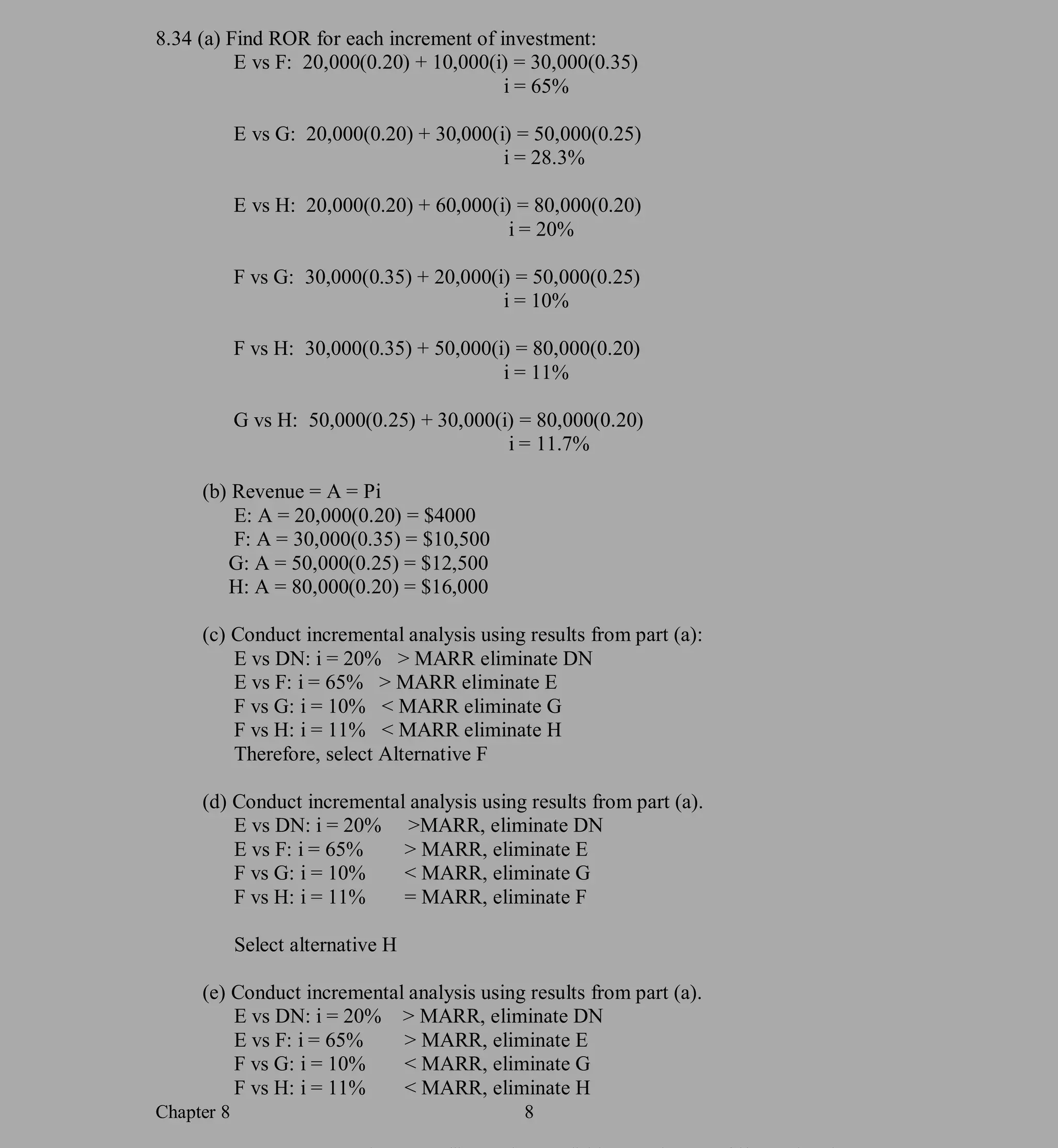
Chapter 8 10
8.41 Answer is (b)
8.42 Answer is (b)
8.43 Answer is (b)
1. PW at 12% is shown in row 29. Select #2 (n = 8) with the largest PW value.
2. #1 (n = 3) is eliminated. It has i* < MARR = 12%. Perform an incremental analysis of
#1 (n = 4) and #2 (n = 5). Column H shows i* = 19.49%. Now perform an
incremental comparison of #2 for n = 5 and n = 8. This is not necessary. No extra
investment is necessary to expand cash flow by three years. The i* is infinity. It is
obvious: select #2 (n = 8).
3. PW at 2000% > $0.05. i* is infinity, as shown in cell K45, where an error for
IRR(K4:K44) is indicated. This analysis is not necessary, but shows how Excel can
be used over the LCM to find a rate of return.
Microsoft Excel - C8 - ext exer soln
®] File Edit View Insert Format Tpols Data Window Help QI Macros
»
B U S % , tog 8 « it _
- H »
iJlFI E
[H « B ffl , Fill Color (Vellow)
1
2
3
4
5
6
7
S
9
10
11
12
13
14
15
IE:
17
18
la
20
21
22
2::;
24
25
A B c E
MARR =
Year
26
0
1
2
3
4
5
E
7
8
9
10
12/t
»1 (n = 3) »1 (n = 4) #2 (n = 5) #2 (n = 8)
Cash flow Cash flow Cash flow Cash tu'.:'
$ (100,000) $ (100,000) $(200,000) $(200,000)
F H
$
|
$
35.000
35.000
35.000
$
$
$
$
35,000
35.000
35.000
35.000
$ 50.000
$ 55.000
$ 80.000
$ 85.000
$ 70.000
$
*
$
$
$
*
$
$
50.000
55.000
80.000
86.000
70.000
70.000
70.000
70.000
11
12
13
14
15
16
17
IS
c
IS
20
au r
Retain or
27 I Eliminate?
28 Incr. i"
29 |pw@12% $
ZASV.
Eliminate
14.96
Retain
14 30%
Retain
25.04%
Retain
(15.336) $ 6.
307 $ 12.224 $ 107.624
#2(6)-to-#l(4)
tt2(n=5) Incremental
20 yr. CP cash flow
$ (100.000) $ (200.000) $
»1
20 yr. CP
J K L M
$
$
$
$
*
$
$
$
*
$
$
$
*
$
$
$
*
$
$
$
35.000 $
35,000 $
35.000 $
(85.000) $
50.000
55.000
80.000
85.000
*
$
$
$
35.000 $ (130.000) $
35.000 » 70.000 $
35.000 $ 70.000 $
(85.000) $ 70.000 $
35.000 $ 70.000 $
35.000 » (130.000) *
35.000 $ 70.000 $
(65.000) $ 70.000 $
35.000 $ 70.000 $
35.000 » 70.000 *
35.000 $ (130.000) $
(65.000) $ 70.000 $
35.000 $ 70.000 $
35.000 » 70.000 *
35.000 $ 70.000 $
35.000 $ 70.000 $
(100.000)
15.000
20.000
25.000
130.000
(165.000)
35.000
35.000
135.000
35.000
(165.000)
35.000
135.000
35.000
35.000
(185.000)
135.000
35.000
35.000
35.000
35.000
1949%
!.<< ! sheetl / Sheet2 / Sheets / Sheet4 / Sheets / Sheet6 / Sheet? / Sheets | 4
»2(8)-to-«2(5)
#2 (n= 5) #2 (n = 8) Incremental
40 gr. CP 40 yr. CP cash flow
$(200,000) $ (200,000) $
s
»
s
$
$ 50.000
$ 55.000
$ 60.000 $
$ 65.000 $
$(130,000)
$ 70.000
$ 70.000 $
$ 70.000 $
$ 70.000
$(130,000)
$ 70.000
$ 70.000
$ 70.000
$ 70.000
s
I
$
$
$
I
$(130,000) $
$ 70.000
$ 70.000
$ 70.000
$ 70.000 $
$(130,000) $
$ 70.000
$ 70.000
$ 70.000 $
$ 70.000 $
$(130,000)
1
$
»
s
I
s
50.000
55.000
80.000
85.000
70.000
70.000
70.000
(130.000)
70.000
70.000
70.000
70,000
70.000
70.000
70.000
(130,000)
70.000
70.000
70.000
70,000
70.000
70.000
70.000
(130.000)
70.000
t
|
$
$
$
|
$
$
$
|
$
$
$
|
$
$
$
|
$
$
$
|
$
$
t
Draw - & | AutoShapes - 0|iil<4l[ll|<9»'i 'A» = 0~
200.000
(200.000)
200.000
200.000
(200.000)
200.000
UUIMJUUI
:i: j ijiji:i
NUM

Chapter 8 11
Case Study 1 Solution
1. Cash flows for each option are summarized at top of the spreadsheet. Rows 9-19 show
annual estimates for options in increasing order of initial investment: 3, 2, 1, 4, 5.
S Miciosoft Excel - ext exei 8.1 soln
® File Edit View Insert Format lools Data Window Help QI Macros
10 - B U
»
A53
A B C D E F G H J K L M
Zi
23
30
31
32
33
34
3!
36
37
38
33
4(1
41
42
il
44
46
Incr. i"
PW@12M $
27
28_
1:)4:)-.
(15.936)
29
3CI
31
32
33
34
t 6.
307 $ 12.224 $ 107,624
35
36
37
38
39
40
Answers
1. Select #2 (n=8)
2. Select #2 (ns 8)
3.
Incrmental i" is infiniti cell K45 giues an error (or IRR(K4:K44)
and PW at large 2000 . is close to jero.)
$ 70.000 $ (130.000) * (200.000)
$(130,000) $ 70.000 $ 200.000
$ 70.000 $ 70.000 $
t Tojoo t nsm $
t Tom t nm $
$ 70.000 t 70.000 $ .
$(130,000) $ 70.000 $ 200.000
$ 70.000 $ 70.000 t
$ 70.000 * (130.000) $ (200.000)
$ 70.000 $ 70.000 $
$ 70.000 $ 70.000 $
$(130,000) $ 70.000 $ 200.000
$ 70.000 t 70.000 $
$ 70.000 t 70.000 $
t 70,000 t nm $
$ 70.000 t 70.000 $
t 70,000 » 7o!oOO $
Incr i1 #DIV(0!
PVat2000X $ 0.05
;gaS'a"| S lfJ F BHP StatusWindow | Mictosott Ence... g|C8-Solulions Mici .| 3 gi.g 11:05AM
C Miciosoft Excel CS Case study 1
Qnlx]
y s a i mm S li 101 ? B U
9
fci - [lil fffi B ffl 5 .
A B L D E F G H
_
T J
1 MAFlFl = 25 ROR. PV. AV analtsis ICa;hr|.:.w;iri:i:1.i:ii:ii])
2 Alternative #2 tti #4 »5
3
4
5
6
7
Initial cost
Est. annual expenses
Est. annual revenues
Sale of business revenue
Lite Year
* *
$-1250.ars1-5
$1150(1-5)
$500(5-8)
10
(400) t (750) t
-
1400(1-5);-2000(6-10) t-800.6x(l|r *
*1400.5x(9r tlOOO K/jr $
(1.000)
(3.000)
3.
500
$
i
(1.500)
(500)
1.
000
10 I 10 10 10
8 Incr. ROR comparisori Actual CF Actual CF Actual CF Actual CF 4-to-3 Actual CF 5-to-4
Incremental investment
Incremental cash flow
0
1
2
3
$0
($100)
($100)
($100)
s
($100)
($400)
to
$70
$144
7
8
3
10
$400
$221
$500
$500
20
21
22
23
24
$.500
$0
$0
$302
($750)
$200
$192
$133
$172
($213)
($124)
($30)
$63
$172
$160
$146
$131
$113
$93
$72
($1,000)
$500
$500
$500
$500
$500
$500
$500
$500
$500
$500
($1,M0)
$600
$600
$600
$600
$100
$0
*0
$0
$500
$500
($1,500)
$500
$500
$500
$500
$500
$500
$500
$500
$500
$500
($500)
$0
to
_
*!_
$o
$o
$0
$0
$0
$0
$0
Qpttofll'
Retain or eliminate?
46.41 :
Retain
10.07X
Eliminate Eliminate
49.08
Retain
31.11M
Retain
Incremental i'
Increment justified?
Alternative selected
49.85K
Yes
#NUMI
Mo
4
25
26
27
28
PW at MARR
AW at MARR
Alternative acceptable?
$215
$60
($152) ($146) $785
Yes
$220
Yes
4
$285
$80
Yes
($500)
T
.ir
MM | | M |ROR, PW, AW analysis f'W calculations / PW vs i / #3 changes / 5heet4 | 4 |
Draw -fed; Auto5hapes »
'
A O |B] SI -s -A SH 0-
Ready ir MUM

Chapter 8 12
3. Do incremental ROR analysis after removing #1 and #2. See row 22. 4-to-3
comparison 4-to-3 yields 59.85%, 5-to-4 has no return because all incremental cash
flows are 0 or negative. PW at 25% is $785.25 for #4, which is the largest PW.
Conclusion: Select option #4 – trade-out with friend.
4. PW vs. i charts for all 5 options are on the spreadsheet.
Options Approximate
compared breakeven____
1 and 2 26%
3 and 5 27
2 and 5 38
1 and 5 42
3 and 4 50
i
i
i;
13
5
-
j
'
i 3=-
5
PW of actual cashflows,
$
9
r -j
1
Tl
o o o o
_
>
0
-
y
-
44:
1 3 9
0 M
El
-
r S
g Q-
5 >N
4
'
-»
n
9-
I
4
:
I ft
44
I -
Tl
5
ITi
4=
i
44-
ft
3
44
mi-
!inr
l>
[a l
< 8

Chapter 8 13
5. Force the breakeven rate of return between options #4 and #3 to be equal to MARR =
25%. Use trial and error or Solver on Excel with a target cell of G22 (to be 25% or
.25 on the Solver window) and changing cell of C6. Make the values in years 5
through 8 of option #3 equal to the value in cell C6, so they reflect the changes. The
answer obtained should be about $1090, which is actually $1,090,000 for each of 4
years.
Required minimum selling price is 4(1090,000) = $4.36 million.
Case Study 2 Solution
1. By inspection only: Select Plan A since its cash flow total at 0% is $300, while Plan B
produces a loss of the same amount ($-300).
2. Calculations for the following are shown on the spreadsheet below.
PW at MARR approach:
PW at 15%: PWA = -$81.38 and PWB = +$81.38. Plan B is selected
PW at 50%: PWA = +$16.05 and PWB = -$16.05. Plan A is selected.
The decisions contradict each other when the MARR is different. It does not seem
logical to accept plan A at a higher interest rate (50%) and at 0%, but reject it at a
mid-point interest rate (15%). The PW at MARR method is not working!
ROR approach:
The cash flow series have two sign changes, so a maximum of two roots may be
found. An ROR analysis using Excel functions for the two plans produce two
identical roots for each plan:
i*1 = 9.51% and i*2 = 48.19%
There are two i* values; it is not clear which value to use for a decision on project
acceptability. Further, when there are multiple i* values, the PW analysis ‘at the
MARR’ does not work, as demonstrated above.

Chapter 8 14
3. Incremental ROR analysis is shown on the spreadsheet below.
Plan B has a larger initial investment than A. The incremental cash flow series (B-
A) has two sign changes. The use of the IRR function finds the same two roots:
9.51% and 48.19%. Incremental ROR analysis offers no definitive resolution.
Miciosofl Excel
to8 >°
8
S I
I Font Color (Red)
-
[m is b m .
A21 = 4
33
C8 - case study 2
A B C D E F
Solution for Case Study 2 - Questions 2 and 3 only
3 n L
1
2. Calculation of FW versus i and determination of I* roots
PLAN A
Year Cashflow Interest. % FW value
5 9.
51%
{300 00
3>1 ,300
-
JS00
SS.OOO
$6,500
5 S111 .60
C»9.36J
C$117.75j
C$119.71)
7 2
'
u i" *1
i« #2
guess -10%
c uess 50%
9.
51%
48.19%
3 20
4 i.4 JU
10 41 r:: Cf65.85) FWat 15% = -3>81 38
1 1 50% t 16 0 5 at 50':::. =
'
j. b 05
1 2
1 ;
1 4
1 5 PLAN B
Interest. %
0%
16 V ear cash flow F'iAi value
1 7 -
f1 ,900
$500
$8,000
.
$6,500
-
$400
C$300.00)
C$111 .80)
$9.36
$117.75
$119.71
$65.85
b 51
1 iE 5.
00%
10.00%
20.00%
30.00%
40.00%
50.00%
guess 10%
IHLIF-: :: 505::
1 H 2 i" #1 9.
51%
48.19%
2L
*
#2
?1
PWat 15% = $81 .38
FWat 50% = -$16.05
2
23 C$16.05)
24
25 Notice that the two plans have identical ROR values.
H N I I FNSheet1 / 5heet2 / Sheets / 5heet4 / Sheets / Sheets / Sheet? / 5 | < |
Draw - & AutoShapes " O O H -41 QS ' 'A-sPMh
15
ir
J L -
Ready NUM
Microsoft Excel
1 Rle Edit
,
A21
A
27
29
20 i ear
L
2
-
4
_
n x
View Insert Format lools Data Window Help QI Macros
10 t B I m M s % , too "o I - a . »
4
il CO - case study 2
B c D E F G H I
3. Incremental ROR analysis
Plan A Plan B Incremental
Cash flow Cash flow cash flow
V ,900
-
J500
-
$3,000
$6,500
$400
-
$1,900
$500
$3,000
-
$6,500
-
$400
-
$3,300
$1,000
$18,000
-
$13,000
-
$800
9.
51%
J K L
i* #1 guess 10% 9.51%
I* #2 guess 50% 48.19%
Twojo°!sL.
LOoJj*ai
FWat 15%= $162.75
FWat 50%= -$32.10
iastaitl g fSP I BHPStat...| @]CaSeSt...| B>ok1 ||[r|C8-C- BjDocum... | gi 9:33AM
-

Chapter 8
4. Composite rate of return approach
Plan A (a) MARR = 15% and c = 15%
F0 = 1900; F1 = 1900(1.15) -500 = 1685; F2 = 1685(1.15) -8000 = -6062.25;
F3 = -6062.25(1+ i') +6500 = 437.75 –6062.25i'
F4 = 0 = F3(1+ i') +400
So i' = 13.06% < MARR = 15%. Reject Plan A.
(b) MARR = 15% and c = 45%
F0 = 1900; F1=1900(1.45) -500 = 2255;
F2 = 2255(1.45) -8000 = -4730.25; F3 = -4730.25(1+ i') +6500 = 1769.75
– 4730.25i' F4 = 0 = F3(1+ i') +400.
So i' = 43.31% > MARR= 15%. Accept Plan A.
(c) MARR = 50% and c = 50%
F0 = 1900; F1 = 1900(1.50) -500 = 2350; F2 = 2350(1.50) -8000 = -4475;
F3 = -4475(1+i') +6500 = -4475i' + 2025
F4 = 0 = F3(1+ i') +400.
So i ' = 51.16% > MARR = 50%. Accept Plan A.
Plan B (a) MARR = 15% and c = 15%
F0 = -1900; F1 = -1900(1+ i') +500; F2 = -1900(1+ i')2
+500(1+ i') +8000;
F3 = (1.15)F2 –6500
F4 = 0 = F3(1.15) -400.
So i' = 17.74% > MARR = 15%. Accept Plan B.
(b) MARR = 15% and c = 45%
F0 = -1900; F1 = -1900(1+i') +500; F2 = -1900(1+ i')2
+500(1+ i') +8000;
F3 = -1900(1.45) (1+ i')2
+500(1.45)(1+ i') +8000(1.45) –6500
F4 = 0 = F3(1.45) - 400.
So i' = 46.14% > MARR = 15%. Accept Plan B
(c) MARR = 50% and c = 50%
F0 = -1900; F1 = -1900(1+ i') +500; F2 = -1900(1+ i')2
+500(1+ i') +8000;
F3 = -1900(1. 5)(1+ i')2
+500(1.5)(1+ i') +8000(1.5) – 6500
F4 = 0 = F3(1.5) - 400.
So i' = 49.30% < MARR = 50%. Reject Plan B.
15
d) Discussion: Plan B is superior to Plan A for c values below i*2, i.e., B’s composite
rate of return is higher. However, for c values above i*2, plan A
gives a higher (composite) rate of return.
Conclusion: The composite rate of return evaluation yields unambiguous results
when a reinvestment rate is specified.

Chapter 9 1
Chapter 9
Benefit/Cost Analysis and Public Sector Economics
9.1 (a) Public sector projects usually require large initial investments while many
private sector investments may be medium to small.
(b) Public sector projects usually have long lives (30-50 years) while private sector
projects are usually in the 2-25 year range.
(c) Public sector projects are usually funded from taxes, government bonds, or user
fees. Private sector projects are usually funded by stocks, corporate bonds, or
bank loans.
(d) Public sector projects use the term discount rate, not MARR. The discount rate
is usually in the 4 – 10% range, thus it is lower than most private sector MARR
values.
9.2 (a) Private (b) Private (c) Public (d) Public (e) Public
(f) Private
9.3 (a) Benefit (b) Cost (c) Cost (d) Disbenefit (e) Benefit (f) Disbenefit
9.4 Some different dimensions are:
1. Contractor is involved in design of highway; contractor is not provided with the
final plans before building the highway.
2. Obtaining project financing may be a partial responsibility in conjunction with
the government unit.
3. Corporation will probably operate the highway (tolls, maintenance,
management) for some years after construction.
4. Corporation will legally own the highway right of way and improvements until
contracted time is over and title transfer occurs.
5. Profit (return on investment) will be stated in the contract.
9.5 (a) Amount of financing for construction is too low, and usage rate is too low to
cover cost of operation and agreed-to profit.
(b) Special government-guaranteed loans and subsidies may be arranged at original
contract time in case these types of financial problems arise later.
9.6 (a) B/C = 600,000 – 100,000 = 1.11
450,000
(b) B-C = 600,000 – 100,000 – 450,000 = $+50,000

Chapter 9 2
9.7 (a) Use Excel and assume an infinite life. Calculate the capitalized costs for all
annual amount estimates.
(b) Change cell D6 to $200,000 to get B/C = 1.023.
File Edit Vie . Insert Formet lools Dete Window Help
-
ft E A SI JJ SB *1 150% -
e# H rf a a * lit B
= -(JF34 tFt5)/(tFt3 i-JFtt,;
_
n x
A B C D G H -
Estimates PW value
20
First cost $
Benefits $
Disbenefits $
Costs $
Discount rate
8,
000,000
550,000
100,
000
800,000
5%
per year
per year
per year
per year
$
$
$
$
8,
000,
000
11,000,000
2,
000,
000
16,000,000
PW = AVWI
= 550.
000/0 05
Note: Since no life is stated, assume it is very long, so the PW
value is the capitalized cost of AW/i.
B/C ratio (B-D)/C 0.
375 |
K < Isheetl/
"
sneet2/
"
Sheets / 1.
| Draw . & | AutoShapes . CD O M -4 IE ' & . -JL . . LlL-.
iiBStart | J% - . > (aj Inbu, - Outl... | feljchoPrub fu... 1 Bjch 9 Solution... | [
"
fMicrosoft E...
E3 Microsoft Excel
Fib Edit View Insert Format Iwls Data Window Help
ft E A Si Si S 150% ,
Aria 10
[ rn
QPriib9.7
.J
b / u * » a a s % , a j?! se « . . a .,
= =(tF(4-JFJ5)/(JFJ3+IFtB)
1
2
3
4
5
6
7
8
9
10
13
A B C D
Estimates PW value
First cost
Benefits
Disbenefits
Costs
Discount rate
$
$
$
8,
000,000
550,000
100,000
$ 200,000
3%
per year
per year
per year
per year
$
$
$
$
8,
000,000
18,333,333
3,
333,333
6,
666,667
B/C ratio . (B-D)/C
14
> W Sheell,;5hsrt2/5heet3/
I
F G
1.
023 I
Note: Since no life is stated, assume it is very long, so the PW
value is the capitalized cost of AW/i.
115Start /] >HH li Inba-.-Oullool'E... | B]Ch 9 Pub for ah ... | B]ch 9 Solulions for ,. Microsoft E«cd iJ-O-i 9''J 300 3'Mm

Chapter 9 3
9.8 1.0 = (12)(value of a life)_
(200)(90,000,000)
Value of a life = $1.5 billion
9.9 Annual cost = 30,000(0.025)
= $750 per year/household
Let x = number of households
Total annual cost, C = (750)(x)
Let y = $ health benefit per household for the 1% of households
Total annual benefits, B = (0.01x)(y)
1.0 = B/C = B/(750)(x)
B = (750)(x)
Substitute B = (0.01x)(y)
(0.01x)(y) = 750x
y = $75,000 per year
9.10 All parts are solved on the spreadsheet once it is formatted using cell references.
E3 Microsoft Excel
File Edit View Insert Format Tools Data Window Help
Cm
Aral .10 . | b / u mmmm s % . a tf ts . «> . a ..
A5 3: = Prob
JPrulj 9.10 .
n x
1
2
3
4
5
6
7
8
9
10
11
12
13
14
15
16
17
18
19
20
21
A B C D E F G H
B/C equation = annual benefit/annual cost J I
For B/C = 1 077
Prob [Median HH income % of HH AW of Cost % affected annual benefit is
9.9 $
9.10a $
9.10b $
30,000 2.50% 750 1% $
18,000 2.0%
30,000 2.5%
360
750
1%
0.
5%
9.10c $ 18,000 2.5% 450 2.50%
$
$
$
75,000
36,000
150,000
18,000
B=$D7/$E7
Answer: Change cell El 3 until $18,000 ishows in F13.
Or, realize the percentage, p, must be 2.5% to obtain 450/p = 18,000.
H < > Isheetl/5heet2/5heet3/
Dra«. (t, I AutoShapes- . Z C 3 4 .
5 $ J, = 11 i'.
J SlartJIl i2l H IB B B 0 |j llnbnic-QutliiokE... | SJch 9 Prob fa 6th ... | B]ch 9 Solutions for ,..|||gMlcrosoft Encel SO'i S S®® 1™™

Chapter 9 4
Note in part (b) how much larger ($150,000) than the median income ($30,000)
the required benefit becomes as fewer households are affected
9.11 (a) Cost = 4,000,000(0.04) + 300,000
= $460,000 per year
B/C = 550,000 – 90,000 = 1.0
460,000
(b) Cost = 4,000,000(0.04)
= $160,000 per year
B - C = (550,000 – 90,000) – (160,000 + 300,000) = 0.0
The project is just economically acceptable using benefit/cost analysis.
9.12 Cost = 150,000(A/P,3%,20) + 12,000
= 150,000(0.06722) + 12,000
= $22,083 per year
Benefits = 24,000(2)(0.50)
= $24,000 per year
B/C = 24,00/22,083 = 1.087
The project is marginally economically justified.
9.13 (a) By-hand solution: First, set up AW value relation of the initial cost, P
capitalized a 7%. Then determine P for B/C = 1.3.
1.3 = 600,000____
P(0.07) + 300,000
P = [(600,000/1.3) – 300,000]/0.07 = $2,307,692
(b) Spreadsheet solution: Set up the spreadsheet to calculate P = $2,307,692.

Chapter 9 5
9.14 Same spreadsheet, except change the discount rate and equations for AW and B/C.
The B/C value is the same at 1.3, so the project is still justified.
0 Microsoft Excel
File Edit View Insert Format lools Data Window Help
a s a u «150% - g.
£ 3 B S % , tig s _
. . A . .
rial r 10 ,
[iKiSryji'd - tEjr.i/tBM
JPn.h 9.13b .
n x
A B C D F G H
2
3 Prob 9.13b
4 Discount rate 7%
5
Annual cost $ 300,000
AW of initial cost (Rate)(P)
Annual benefit $ 600,000
B/C ratio 1.30
6
7
8
9 P = (($B$8/$B$9) - $B$6)/SB$4
10
11 Initial cost, P 2,
307,692
12
13
14
15
16
< < > WNSheetli Sheflz/Sheets/
L .
] Draw- k & «05hape!- O B 4 ffl <2». ;.A
gStart > @ H Intt... -Outloul E,, jjjCh 9 Piob in tth .J lajrh 9 Sulutons in ,.,| Microsoft Excel ' O i .w
'
5:32 PH
-
10 - I B y u .- - - Hi -x. , tiS I « * I B3 - g! - A. - -I
3 =1-
_
:n x
A C D
1
3 Prob 9.13b Prob 9.14
4 Discount rate 7% 5%
$ 300,000
(Rate)(P)
$ 600,000
1.
30
s
Annual cost
AW of initial cost
300,000
AW CI 1*C4
S
7 161,500
8 Annual benefit
B/C ratio
S 600,
000
30
B/C C8/(C6+C7)
10
1 1 Initial cost, P 2,
307,692 S 3,
230,
000
1 2
13
[A 5heet2 / Sheets /
Draw » AutoShapes x > o Ml 41 ii; a - = - s a |_
.
jgastartjlj 3 1 Bjj (B| E IM JInbox-OuHookE...j @]Ch 9 Prob for fith... | Sjch 9 Solutions fo... | || Microsoft Erreel SSvO i t .?i®,S ! 6:27 PM

Chapter 9 6
9.15 1.7 = 150,000 – M&O costs_
1,000,000(A/P,6%,30)
1.7 = 150,000 – M&O costs
1,000,000(0.07265)
M&O costs = $26,495 per year
9.16 Convert all estimates to PW values.
PW disbenefits = 45,000(P/A,6%,15)
= 45,000(9.7122)
= $437,049
PW M&O Cost = 300,000(P/A,6%,15)
= 300,000(9.7122)
= $2,913,660
B/C = 3,800,000 – 437,049__
2,200,000 + 2,913,660
= 3,362,951/5,113,660
= 0.66
9.17 (a) AW of Cost = 30,000,000(0.08) + 100,000
= $2,500,000 per year
B/C = 2,800,000 = 1.12
2,500,000
Construct the dam.
(b) Calculate the CC of the initial cost to obtain AW for denominator.
B/C = 1.12
B/C = (2,800,000)/(100,000+30,000,000*(0.08))

Chapter 9 7
9.18 AW = C = 2,200,000(0.12) + 10,000 + 65,000(A/F,12%,15)
= 264,000 + 10,000 + 65,000(0.02682)
= $275,743
Annual Benefit = B = 90,000 – 10,000 = $80,000
B/C = 80,000/ 275,743 = 0.29
Since B/C < 1.0, the dam should not be constructed.
9.19 Calculate the AW of initial cost, then the 3 B/C measures of worth. The roadway
should not be built.
Microsoft Excel - Prob 9.19
l§j File Edit View Insert Format Tools Data Window Help -
Ifflxll
b / u mmmm s % . td8 8 tf if _
. ». a ..
L
: -
L
B D F G H J
Given:
Initial cost $ 18.
000,
000
Annual upkeep $ 150,
000
2 (a)
3 - C method B/C method
(c)
Mod B/C method
3
4
Annual benefits
5 900,000 $819,322)
Don't build
j 47ft
J e'ft
ft
Discount rate
Useful life, yrs
ftri: Don't build Don't build
8 ft
0 Calculated:
AWof initial cost $1,
569,322
F I5>1, "Build",
"
Don't build"
F E5>0,
"
Build","Don't build"
11
Ift
3
14
I-ft
B-L ;C5)- (C11 + C3) Vied B/C ;C5- C3)/C11
17
I -
Ift
ftll
2
22
_
ft
4
li i l5heeH/5heet2/Sheets / <
D,a». k & AutoShapes- Z C 4 ,
5 .J. A =
Page 4 Sec 1 4/M At 1" [ill Col 19 [REC pT fW |0VR | |y3 I
ii8st''rt I 4] fe O l> B B SI 'l! | Microsoft Emel - Prob... SQch 9 Prob for 6th - Micros... | B]ch 9 Solutions for 6th - Mi...j S&O'-J IWI«H

Chapter 9 8
9.20 (a) AW = C = 1,500,000(A/P,6%,20) + 25,000
= 1,500,000(0.08718) + 25,000
= $155,770
Annual revenue = B = $175,000
B/C = 175,000/155,770 = 1.12
Since B/C > 1.0, the canals should be extended.
(b) For modified B/C ratio,
C = 1,500,000(A/P,6%,20) = $130,770
B = 175,000 – 25,000 = 150,000
Modified B/C = 150,000/130,770
= 1.15
Since modified B/C > 1.0, canals should be extended.
9.21 (a) Determine the AW of the initial cost, annual cost and recurring dredging cost,
then calculate (B – D)/C.
Microsoft Excel - Prob 9.21
Igj File Edit View Insert Format Tools Data Window Help
Anal T 10 T
H9
B / u a @ S % , tsS 8 tF * _
' A . .
=(H5-H3)/E24
A B C D E H I J
1
2 Year
3
4
5
6
_
7
_
_
9
_
10
il
J2
JI3
14
15
ii
17
18
ii
20
21
22
23
24
25
26
Initial cost Annual cost Dredging cost Total cost
0
1
2
3
4
1,
500,000
5
6
7
8
9
10
11
12
13
14
15
16
17
18
19
20
AW value
25,
000
25,000
25,000
25,
000
25,000
25,
000
25,
000
25,000
25,
000
25,000
25,000
25,
000
25,000
25,000
25,
000
25,000
25,
000
25,
000
25,000
25,
000
60,000
60,
000
60,
000
60,
000
60,
000
60,
000
1,
500,000
25,
000
25,000
85,
000
25,
000
25,000
85,
000
25,000
25,000
85,
000
25,000
25,000
85,
000
25,000
25,
000
85,
000
25,
000
25,
000
85,000
25,000
25,
000
Annual disbenefit $ 15.000
Annual revenue $ 175.
000
B/C = 0 922 I
$173,568
AW = -PMT(6%,20,NPV(6%,E4:E23)+E3)
14 < >l5heetl / sheeE >rsheet3 /
Draw . AutoShapK . DOH HBl*- - A . S L -
Page 8 Sec 1 8/22 |At 2.3" in 8 col 2 [rec [trk pxf f5vR flj:
1J Microsoft EHcel - Prob... E]Ch 9 Prob for 6th - Micros... | ®]Ch 9 Solutions for 6th - Mi,, 12142 PM

Chapter 9 9
The disbenefit of $15,000 per year and the dredging cost each third year have
reduced the B/C ratio to below 1.0; the canals should not be extended now.
(b) AW = C = 1,500,000(A/P,6%,20) + 25,000 + 60,000(P/F,6%,3) + (P/F,6%,6)
+ (P/F,6%,9) + (P/F,6%,12) + (P/F,6%,15) + (P/F,6%,18)(A/P,6%,20)
= 1,500,000 (0.08718) + 25,000 + 60,000 0.8396 + 0.7050 + 0.5919 +
0.4970 + 0.4173 + 0.3503(0.08718)
= $173,560
Annual disbenefit = D = $15,000
Annual revenue = B = $175,000
(B – D)/C = (175,000 – 15,000)/173,560 = 0.922
As above, the disbenefit of $15,000 per year and the dredging cost each third
year have reduced the B/C ratio to below 1.0; the canals should not be
extended now.
9.22 Alternative B has a larger total annual cost; it must be incrementally justified. Use
PW values. Benefit is the difference in damage costs. For B incrementally over A:
Incr cost = (800,000 – 600,000) + (70,000 – 50,000)(P/A,8%,20)
= $200,000 + 20,000(9.8181)
= $396,362
Incr benefit = (950,000 – 250,000)(P/F,8%,6)
= 700,000(0.6302)
= 441,140
Incr B/C = 441,140/396,362
= 1.11
Select alternative B.
9.23 Annual cost of long route = 21,000,000(0.06) + 40,000 + 21,000,000(0.10)
(A/F,6%,10)
= 1,260,000 + 40,000 + 2,100,000(0.07587)
= $1,459,327
Annual cost of short route = 45,000,000(0.06) + 15,000 + 45,000,000(0.10)
(A/F,6%,10)
= 2,700,000 + 15,000 + 4,500,000(0.07587)
= $3,056,415

Chapter 9 10
The short route must be incrementally justified.
Extra cost for short route = 3,056,415 – 1,459,327
= $1,597,088
Incremental benefits of short route = 400,000(0.35)(25 – 10) + 900,000
= $3,000,000
Incr B/Cshort = 3,000,000
1,597,088
= 1.88
Build the short route.
9.24 Justify extra cost of downtown (DT) location.
Extra cost for DT site = 11,000,000(0.08)
= $880,000
Extra benefits for DT site = 350,000 + 400,000
= $750,000
Incremental B/CDT = 750,000/880,000
= 0.85
The city should build on the west side site.
9.25 East coast site has the larger total cost (J17). Set up the spreadsheet to calculate
AW values in $1 million. First, perform B/C on west coast site since do-nothing is
an option. It is justified. Then use incremental values to evaluate East versus
West. It is also justified since Δ(B/C) = 2.05. Select east coast site.
]p h di's a y | x to e- l
I Ariai .10 . | b / a m mmm S % . to8 8 » * - <5» - A ..
.
.
x
LI 3 = =Mii/Hg
.
x,
A B : F H J K L
.
'
'
.
'
t
'
i
'
1 _
c n lt Li:e East Coast Site
2 Imt a
cost
Annua
M8.0
I nt a I
: osts
Initial
cost
Annua otal
costs
J Tear J'
-
erlg nil .
'
:u iit
: 3 r 12 20 0 [B-Dl/C of West
1.
51 0 8 B.S
0,
8 0.B
I L 2.
29 Justified
2 i e
5
=astv. West
J 1 5 I : I .
J t
i
=
I 2 1 F 2 r ncremental (B-D)/C
fr 24c
I - L1L =
LI _
'
1.
6 3.
6 J L J I:
4B=/$ D.5D0
2.05/ IJustlfied
I I b I J : .
I:
I 32
12 1 5 I C J :
.
5 I 5
13 J ; J I:
14 J i 5 I G J ; .
I:
6 ! I 5 15 J : J I:
3.
7
4;i 12 -
2 I 5
I 5
I 6
1.
5
I 5
I 5
I 5
1 5
1 5
J : .
I:
I2L-D2LIHI 7-C2 |
17 3 I 5 H 33
3 1 5
14
3 I 3
113 I 5
1 5
3 92
AA
I 5
AW = -Pm«26,12,NPVBL$2B,J5:J16 +J4
31
32 3:1 342
3:1
24 41
AW value
Benefits 5 mil@ 2.50 =
Disbeneflts
25
26
H
28
Draw - 1 Qj Auto5hapes
125
4
$3.72-
AW = -(PMT($L$26,20,NPV($L$26,E5:E24)+E4))|
8 mil® 2 00 = 13 Disc rate 43

Chapter 9 11
9.26 First compare program 1 to do-nothing (DN).
Cost/household/mo = $60(A/P,0.5%,60)
= 60(0.01933)
= $1.16
B/C1 = 1.25/1.16
= 1.08 Eliminate DN
Compare program 2 to program 1.
Δcost = 500(A/P,0.5%,60) – 60(A/P,0.5%,60)
= (500 – 60)(0.01933)
= $8.51
Δbenefits = 8 – 1.25
= $6.75
Incr B/C2 = 6.75/8.51
= 0.79 Eliminate program 2
The utility should undertake program 1.
9.27 Using the capital recovery costs, solar is the more costly alternative.
Δcost = (4,500,000 – 2,000,000)(A/P,0.75%,72)
– (150,000 – 0)(A/F,0.75%,72)
= 2,500,000(0.01803) – 150,000(0.01053)
= $43,496
Δbenefits = 50,000 – 10,000
= $40,000
Incr B/C = 40,000/43,496 = 0.92
Select the conventional system.
9.28 (a) Location E
AW = C = 3,000,000(0.12) + 50,000
= $410,000
Revenue = B = $500,000 per year
Disbenefits = D = $30,000 per year

Chapter 9 12
Location W
AW = C = 7,000,000 (0.12) + 65,000 - 25,000
= $880,000
Revenue = B = $700,000 per year
Disbenefits = D = $40,000 per year
B/C ratio for location E:
(B – D)/C = (500,000 – 30,000)/410,000
= 1.15
Location E is economically justified. Location W is now incrementally
compared to E.
Δcost of W = 880,000 – 410,000
= $470,000
9.28 (cont) Δbenefits of W = 700,000 – 500,000
= $200,000
Incr disbenefits of W = 40,000 – 30,000
= $10,000
Incr B/C = (B – D)/C = (200,000 – 10,000)/470,000
= 0.40
Since incr(B – D)/C < 1, W is not justified. Select location E.
(b) Location E
B = 500,000 – 30,000 – 50,000 = $420,000
C = 3,000,000 (0.12) = $360,000
Modified B/C = 420,000/360,000 = 1.17
Location E is justified.
Location W
ΔB = $200,000
ΔD = $10,000
ΔC = (7 million – 3 million)(0.12)
= $480,000
ΔM&O = (65,000 – 25,000) – 50,000
= $-10,000
Note that M&O is now an incremental cost advantage for W.
Modified ΔB/C = 200,000 – 10,000 + 10,000 = 0.42
480,000 W is not justified; select location E.

Chapter 9 13
9.29 Set up the spreadsheet to find AW of costs, perform the initial B/C analyses using
cell reference format. Changes from part to part needed should be the estimates
and possibly a switching of which options are incrementally justified. All 3
analyses are done on a rolling spreadsheet shown below.
(a) Bob: Compare 1 vs DN, then 2 vs 1. Select option 1.
(b) Judy: Compare 1 vs DN, then 2 vs 1. Select option 2.
(c) Chen: Compare 2 vs DN, then 1 vs 2. Select option 2 without doing the ΔB/C
analysis, since benefits minus disbenefits for 1 are less, but this option has a
larger AW of costs than option 2.
9.29 (cont)
I LiJJ.U.IJJNJ.i
IS] File Edit View Insert Format lools Data Window Help
Aria! - 10 - B U s
125% 13 -
K48
A B C I D T E T F I G H I I J K 1
1 Part (a) Analysis by Engineer Uab
2
3
4
5
6
7
_
8
g
10
12
Discount rate 10%
Option 1 Option 2
Initial cost, $
Cost. $/yr
AW of costs. $/yr
Benefits.
$/yr
Disbenefits. $/yr
Life, yrs
50.000
3.
000
16.
190
20.000
500
5
90.
000
4.
000
27.
742
29.
000
1.
500
5
1 vs DN
Delta C
Delta B
Delta D
Delta B/C
16.190
20.
000
500
1 20 Do 1
2 vs 1
I I ,
552
j.
ijijj
Delta B/C = ($G9-$G10)/$G8
IF($G12>1.,,Do 2"."Do 1")
u 69 Do 1
13 Part (b) Analysis by Engineer Judy
14
15
16
17
18
19
20
21
22
23
24
Discount rate I 0%
Option 1 Option 2
Initial cost.
$
Cost. $/yr
AW of costs. $/yr
Benefits. $/yr
Disbenefits. $/yr
Life, yrs
75.
000
3.
800
23.585
30.000
1.
000
1
90.
000
3.
000
26.742
35.000
0
5
1 vs DN 2 vs 1
Delta C
Delta B
Delta D
Delta B/C
23,585
30.000
1000
1.
23 Do 1
3.
157
5.
000
-
1.
000
1 90 Do 2
! <]< I I WlSheetl / 5heet2 / Sheets /
Draw - Auto5hape5 - O H] *4l LSi
| At 7" Ln 34 CoTl | KL _ | i h:>
= = e g .|
i' i
I-
-
i y<i
Page 6 6/14
igBstai-t I _
J3 .:J > 01] S !|i m) |] i lInbox-QutlookE.-, | Ejch 9 Prob for 6th ... | I MicrosoFt Excel BjCh 9 Solutions for .. .| 0'
.
2)Sl

Chapter 9 14
9.30 Find the AW of costs for each technique, order them, and determine the Incr B/C
values.
AW of costs = installed cost(A/P,15%,10) + AOC
9.30 (cont)
Technique AW of cost calculation__
1 15,000(A/P,15%,10) + 10,000
= 15,000(0.19925) + 10,000
= $12,989
2 19,000(A/P,15%,10) + 12,000
= 19,000(0.19925) + 12,000
= $15,786
3 25,000(A/P,15%,10) + 9,000
= 25,000(0.19925) + 9,000
= $13,981
4 33,000(A/P,15%,10) + 11,000
= 33,000(0.19925) + 11,000
= $17,575
ISJ File Edit View Insert Format lools Data Vtfndow tlelp
J p os h « a & m a f | .o - o- a IiBra 'z5-''- - gi-I
mm m as , taS j * * | _ . «. . .
.10 - n
E37
-
= | =($E34-tE35)/IE33
T
A B C D E F G J K
26 Part (c) Analysis by Engineer Chen. Must switch order of comparison to 1 vs 2
27
28
Discount rate I 0%
Option 1 Option 2
31 Initial cost, $
32 Cost, $/yr
33 AW of costs, $/yr
34 Benefits, $/yr
35 Disbenefits,
$/yr
36 Life, yrs
37
39
4U
4 1
60.
000
6.
000
2 1,
828
30.
000
5.
000
5
70,
000
3,
000
21,466
35,
000
1 ,
000
5
2 vs DN
Delta C
Delta B
Delta D
21 ,466
35,
000
1.
000
Delta B/C | 1.S8 | Do 2
4,
01. Li
-
24 86
| = IF($E38>1 ,"Do 2","Do
Do 2
AW of costs = -(PMT($B27,$B36.
-
PV($B27.
$B36,$B32)+$B31))
Not a meaningful B/C value since option 1
has larger AW of costs, but provides a
lower (B-D) value. Incremental analysis
not needed,
simply select option 2
i e g -I
hi
j JInbox - OutlookE | Ch 9 Prob for 6th ... |[[ Microsoft Ewcet BjCh 9 Solutions for ...| O'
O Kl ©"©.3)
| Page 13 Sec 1 13(23 i At 7.6" Ln 13 Col I
12;45 PM

Chapter 9 15
Order of incremental analysis is: DN, 1, 3, 2, 4.
Technique 1 vs DN (current)
B/C = 15,000/12,989
= 1.15 > 1.0 Eliminate DN, keep technique 1.
Technique 3 vs 1
C = 13,981 – 12,989 = $992
B = 19,000 – 15,000 = $4,000
B/C = 4,000/992
= 4.03 > 1 Eliminate technique 1, keep 3.
Technique 2 vs 3
C = 15,786 - 13,981 = $1,805
B = 20,000 – 19,000 = $1,000
B/C = 1,000/1,805
= 0.55 < 1.0 Eliminate technique 2, keep 3.
Technique 4 vs 3
C = 17,575 - 13,981 = $3,594
B = 22,000 -19,000 = $3,000
B/C = 3,000/3,594
= 0.83 < 1.0 Eliminate technique 4, keep 3
Replace the current method with technique 3.
9.31 Determine the AW of costs for each technique and calculate overall B/C. Select
all four since all have B/C > 1.0.
1 A B C D E
2 Technique 1 2 3 4
3
4 Installed cost 15,000 19,000 25,000 33,000
5 AOC 10,000 12,000 9,000 11,000
6 AW of costs $12,989 $ 15,786 $ 13,981 $ 17,575
7
8 Benefits 15,000 20,000 19,000 22,000
9
10 B/C 1.15 1.27 1.36 1.25
11
12 Select? Yes Yes Yes Yes
AW of costs = E$5 - PMT(15%,10,E$4)

Chapter 9 16
9.32 Combine the investment and installation costs, difference in usage fees define
benefits. Use the procedure in Section 9.3 to solve. Benefits are the incremental
amounts for lowered costs of annual usage for each larger size pipe.
1, 2. Order of incremental analysis: Size 130 150 200 230
Total first cost, $ 9,780 11,310 14,580 17,350
3. Annual benefits, $ -- 200 600 300
4. Not used since the benefits are defined by usage costs.
5-7. Determine incremental B and C and select at each pairwise comparison of
defender vs challenger.
150 vs 130 mm
C = (11,310 – 9,780)(A/P,8%,15)
= 1,530(0.11683)
= $178.75
B = 6,000 – 5,800
= $200
B/C = 200/178.75
= 1.12 > 1.0 Eliminate 130 mm size.
200 vs 150 mm
C = (14,580 – 11,310)(A/P,8%,15)
= 3270(0.11683)
= $382.03
B = 5800 – 5200
= $600
B/C = 600/382.03
= 1.57 > 1.0 Eliminate 150 mm size.
230 vs 200 mm
C = (17,350 – 14,580)(A/P,8%,15)
= 2770(0.11683)
= $323.62
B = 5200 – 4900
= $300
B/C = 0.93 < 1.0 Eliminate 230 mm size.
Select 200 mm size.

Chapter 9 17
9.33 Compare A to DN since it is not necessary to select one of the sites.
A vs DN
AW of Cost = 50(A/P,10%,5) + 3
= 50(0.26380) + 3
= 16.19
AW of Benefits = 20 – 0.5
= 19.5
B/C = 19.5
16.19
= 1.20 > 1.0 Eliminate DN.
B vs A
C = (90 – 50)(A/P,10%,5) + (4 – 3)
= 40(0.26380) + 1
= $11.552
B = (29 – 20) – (1.5 – 0.5) = 8
B/C = 8/11.552
= 0.69 < 1.0 Eliminate B.
C vs A
C = (200 – 50)(A/P,10%,5) + (6 – 3)
= 150(0.26380) + 3
= 42.57
B = (61 – 20) – (2.1 – 0.5) = 39.4
B/C = 39.4/42.57
= 0.93 < 1.0 Eliminate C
Select site A
9.34 (a) Calculate the B/C of each proposal for initial screening (row 6). Four
locations are retained – F, D, E and G. No need to compare F vs DN since
one site must be selected. Site D is the one selected.

Chapter 9 18
(b) For independent projects, use the B/C values in row 6 of the Excel solution
above and select the largest three of the four with B/C > 1.0. Those selected
for are: D, F, and E.
9.35 (a) An incremental B/C analysis is necessary between Y and Z, if these are
mutually exclusive alternatives.
(b) Independent projects. Accept Y and Z, since B/C > 1.0.
9.36 J vs DN
B/C = 1.10 > 1.0 Eliminate DN.
K vs J
B/C = 0.40 < 1.0 Eliminate K.
S] File Edit View Insert Format Tools Data Window Help JBJX]
anal 10
GU 3
b / u mmmm s % , r«8 8 «« . «.. a ..
A B c D E F G H I J K
2
Loan rate, %/year
Location
4%
F B D E G C
3 jFirst cost, $ million
4
_
Cap rec cost. $100.000
5
_
Benefits, $/year
6 Site B/C (initial screening)
7 Retain?
8
9
10
11
12
6 i 8 9 I 12 14 | 18 1 22
240,000 _
32Cl.000
_
360 000 480,000 560,000 | 720.000 880.000v i 1
390,
000 310,
000 800,000 750,
000 400.
000 930,
000 850,000 =H$3'
innnnnn«$B$1
1.
63 0.97 ITzTT iMl OTTl 1291 osTT
Retain No
Comparison
Inc. cap rec cost
Inc benefits
Inc B/C value
Retain Retain
D vs F Evs D
120,
000 120,000
410,000 lower
No
13 Incrementjustified?
14 Site selected
15
16
17
18
li
20
21
22
23
24
25
26
3.
42
Yes
D
No
D
Re:;: n
GvsD
360,000
130,
000
No
0 36
No
=IF(H$6>1,
"
Retain,,,
,,
No")
Draw, | AutoStiapes. DOil4[l dl.i£. . = jsglg1.|
1
H m
E I
Page 17 Sec 1 17/24 « 2.1" | REC |TRi: |EXT |OVR 1 SS
.
jlnbo>-QutlookE...| r|Ch9Probfor6th...||gMlcrosQftE>lcel... BJch9Solutionsfo... | SO N 10:10m
In 7 Col 1

Chapter 9 19
L vs J
B/C = 1.42 > 1.0 Eliminate J.
M to L
B/C = 0.08 < 1.0 Eliminate M.
Select alternative L.
Note: K and M can be eliminated initially because they have B/C < 1.0.
9.37 (a) Projects are listed by increasing PW of cost values. First find benefits for each
alternative and then find incremental B/C ratios:
Benefits for P
1.1 = BP /10
BP = 11
Benefits for Q
2.4 = BQ/40
BQ = 96
Benefits for R
1.4 = BR/50
BR = 70
Benefits for S
1.5 = BS/80
BS = 120
Incremental B/C for Q vs P
B/C = 96 – 11
40 – 10
= 2.83
Incremental B/C for R vs P
B/C = 70 – 11
50 – 10
= 1.48
Incremental B/C for S vs P
B/C = 120 – 11
80 – 10
= 1.56

Chapter 9 20
Incremental B/C for R vs Q
B/C = 70 – 96
50 – 40
= -2.60
Disregard due to less B for more C.
Incremental B/C for S vs Q
B/C = 120 – 96
80 – 40
= 0.60
Incremental B/C for S vs R
B/C = 120 – 70
80 – 50
= 1.67
(b) Compare P to DN; eliminate DN.
Compare Q to P; eliminate P.
Compare R to Q; disregarded.
Compare S to Q; eliminate S.
Select Q.
FE Review Solutions
9.38 Answer is (d)
9.39 Answer is (b)
9.40 Answer is (a)
9.41 Answer is (c)
9.42 Project B/C values are given. Incremental analysis is necessary to select one
alternative. Answer is (d)
9.43 Answer is (c)
9.44 Answer is (a)

Chapter 9 21
Extended Exercise solution
1. The spreadsheet shows the incremental B/C analysis. The truck should be
purchased. The annual worth values for each alternative are determined using the
equations:
AWpay-per-use = 150,000(A/P,6%,5) + 10(3000) + 3(8000) = $89,609 (cell D15)
AWown = 850,000(A/P,6%,15) + 500,000(A/P,6%,50) + 15(2000) + 5(7000)
= $184,240 (cell F15)
2. The annual fee paid for 5 years now would have to be negative (cell D5) in that
Brewster would have to pay Medford a ‘retainer fee’, so to speak, to possibly use the
ladder truck. This is an economically unreasonable approach.
Excel SOLVER is used to find the breakeven value of the initial cost when B/C = 1.0
(cell F21).
S Microsoft Excel
I-|n|x
3
il Em Exer 9 (soln) X
2l
A E c G H I
1
3
4
5
Extended Exercise solution (4 sheets in this workbook)
Discount rate = 6%
Alternative
#1
Pay per use
#2
Own
1) Original scenario
_
i_
j K L M N -
9
JO
Jl
13
H
Initial cost,
%
Life, years
Building cost
Building life, years
AW of initial costs
# dispatches/year
$150,000
5
$ 850,000
15
$ 500,000
Dispatch cost,
$/event
# activations/year
Activation cost, $Jevent
15 AW of costs, S ear
10
$ 3,000
3
$8,000
$89,609
50 +
15
$ 2,000
5
$7,000
$184,240
jejPremium reduction, $/year
jrJPi'operty loss reduction, $/year
13 AW of benefits, tiyear
19 Alternatives compared
lol Incremental costs (delta C)
21 Incremental benefits (delta B)
22
23
24
$1 00,000
$300,000
$400,000
$200,000
$400,000
$600,000
Incremental B/C ratio
2-to-1
$94,631
$200.000
2 11
Yes
i y Hquestion#l/ Question #2 / Question #3 / Question #4 / sheets /sh(|4 I
Draw - AutoShapes - O HMl Si .2»-i 'A. = 5nn;gQ|_
,
Ready MUM

Chapter 9 22
3. The building cost of over $2.2 million could be supported by the Brewster proposal
(in cell F7), again found by using SOLVER. This is also not an economically
reasonable alternative.
Miciosoft Excel
IEx
D & H
I
10 T B / 1 $ % , tjg X J -A .
A23 =
P Ext Exei 9 (soln) HE
2
3
4
A B C D E F G H I J K L
Discount rate = 6% 2) Reduce annual fee (cell D5)
#1 #2
Alternative Pay per use Own
5
6
7
8
9
10
11
12
13
14
Initial cost,
S ($301,1 07)
Life,
years
Building cost
5
J 850,000
15
% 500,000
50+
AW of initial costs
tfdispatches/year
Dispatch cost,
$/event
# activations/year
Activation cost, I/event
AW of costs, Syear
10 15
% 3,000
3
18,000
($17,482)
I 2,000
5
$7,000
$182,518
15
16
17
Premium reduction,
$/vear $1 00,000
Property loss reduction, $iVear $300,000
AW of benefits, JiVear $400,
000
$200,000
$400,000
$600,000
IS
10
20
Alternatives compared
Incremental costs (delta C)
Incremental benefits (delta B)
2-to-1
$200,000
$200,000
21
22
Incrementjustified?
1.
00
No
N lVl H M [ Question #1 Question #2 / Question #3 / Question #4 / Sheets / Shi M
] Draw (t; | AytoShapes O 1 ll ii'A.s Q
Ready
'
InUmT

Chapter 9 23
4. The estimated sum of premium and property loss would need to be $523,714 or less
(cell F17, SOLVER). This is not much of a reduction from the current estimate of
$600,000.
Microsoft Excel
y #a 10 w B / $ % , to?
.0 .00
+ .0
. A , »
A23
ijExtExer9(soln)
A B
1
2
3
Discount rate = 6%
_
c d | e | F
3) Increase building cost
G H I J K L M N -
Alternative
#1
Pay per use
#2
Own
5
E
7
8
9
10
11
12
13
14
Initial cost,
$
Life, years
Building cost
AW of initial costs
# dispatches/year
Dispatch cost,
(f/event
# activations/year
Activation cost,
$/event
AW of costs, $Vear
$150,000
5
$ 850,000
15
10
$2,284,353
50 +
15
'
i 3,
000
3
$8,000
$89,609
$ 2,000
5
$7,000
$289,610
15
16
17
Premium reduction, $/year $100,000 $200,000
Property loss reduction, $/Vear $300,000 $400,000
AWof benefits, $Vear | $400,
000 $600,
000
18
19
20
I
2-to-1
$200,000
$200,000
21
22
r
1.
00
No
| MIX Question*l / Question#2 question #3 / Question*4 /Sheets /Shi | < | I
I Draw ' (t> | AutoShapes " O H 41 ill ' 'A s
Ready
L
NUM
r

Chapter 9 24
Case Study Solution
1. Installation cost = (3,500)87.8/(0.067)(2)
= (3,500)(655)
= $2,292,500
Annual power cost = (655 poles)(2)(0.4)(12)(365)(0.08)
= $183,610
Total annual cost = 2,292,500(A/P,6%,5) + 183,610
= $727,850
If the accident reduction rate is assumed to be the same as that for closer spacing of
lights,
B/C = 1,111,500/727,850
= 1.53
[3 Miciosolt Excel
X
11 - B / , A , »
J
Ml
Q]jExtExei9(soln)
_
i
_
2
3
4
5
6
7
8
Id
II
12
13
14
15
Ji
j?
18
J9
20
A I B I C
Discount rate = 6%
E F G H I J K L
Alternative
4) Reduce: initial fee by 50%,
event cost to
level of'own'.
Increase Ins. benefits
SI #2
Own
Initial cost, $
Life, years
Building cost
AW of Initial costs
# dispatches/year
Dispatch cost, Wevent
# activations/year
Activation cost, $/event
AW of costs, jyear
Pay pet use
I $75.000 I
5
1850,000
15
J500,000
50+
M
J.
_
K-|
10
$ 2,000
15
3
:ii7,ij[iij |
mm
$ 2,000
5
$7,000
$182,518
Premium reduction, $/year $100,000
Properly loss reduction, $/year $300,000
AW of benefits, { year $400,000
$200,000
$400,000
$523,714
2-to-1
$123,714
$123,714
21 Incremental B/C ratio
a|Incrementjustified?
I on
22 [Incrementjustified? | | | No | |
H < |HN Question#1 / Question#2 / Question#3 Question #4/Sheets /Shi 14 2JJ1
-
Draw * k AutoShapes' OH llll - 'A s gljl,
"
'
eddy NUM

Chapter 9 25
2. Night/day deaths, unlighted = 5/3 = 1.6
Night/day deaths, lighted = 7/4 = 1.8
3. Installation cost = 2,500(87.8/0.067)
= $3,276,000
Total annual cost = 3,276,000(A/P, 6%, 5) + 367,219
= $1,144,941
B/C = 1,111,500/1,144,941
= 0.97
4. Ratio of night/day accidents, lighted = 839 = 0.406
2069
If the same ratio is applied to unlighted sections, number of accidents prevented
where property damage was involved would be calculated as follows:
0.406 = no. of accidents
379
no. accidents = 154
no. prevented = 199 –154 = 45
5. For lights to be justified, benefits would have to be at least $1,456,030 (instead of
$1,111,500). Therefore, the difference in the number of accidents would have to be:
1,456,030 = (difference)(4500)
Difference = 324
No. of accidents would have to be = 1086 – 324 = 762
Night/day ratio = 762 = 0.368
2069

Chapter 10 1
educators permitted by McGraw-Hill for their individual course preparation. If you are a student using this Manual, you are using it without
permission.
Chapter 10
Making Choices: the Method, MARR, and Multiple Attributes
10.1 The circumstances are when the lives for all alternatives are: (1) finite and equal, or (2)
considered infinite. It is also correct when (3) the evaluation will take place over a specified
study period.
10.2 Incremental cash flow analysis is mandatory for the ROR method and B/C method. (It is
noteworthy that if unequal-life cash flows are evaluated by ROR using an AW-based
relation that reflects the differences in cash flows between two alternatives, the breakeven i*
will be the same as the incremental i*. (See Table 10.2 and Section 10.1 for comments.)
10.3 Numerically largest means the alternative with the largest PW, AW or FW identifies the
selected alternative. For both revenue and service alternatives, the largest number is chosen.
For example, $-5000 is selected over $-10,000, and $+100 is selected over $-50.
10.4 (a) Hand solution: After consulting Table 10.1, choose the AW or PW method at 8% for
equal lives of 8 years.
Computer solution: either the PMT function or the PV function can give single-cell
solutions for each alternative.
In either case, select the alternative with the numerically largest value of AW or PW.
(b) (1) Hand solution: Find the PW for each cash flow series.
PW8 = -10,000 + 2000(P/F,18%,8) + (6500 – 4000) (P/A,18%,8)
= -10,000 + 2000(0.2660) + 2500(4.0776)
= $726
PW10 = -14,000 + 2500(P/F,18%,8) + (10,000 – 5500) (P/A,18%,8)
= $5014
PW15 = -18,000 + 3000(P/F,18%,8) + (14,000 – 7000) (P/A,18%,8)
= $11,341

Chapter 10 2
PW20 = -24,000 + 3500(P/F,18%,8) + (20,500 – 11,000) (P/A,18%,8)
= $15,668
PW25 = -33,000 + 6000(P/F,18%,8) + (26,500 – 16,000) (P/A,18%,8)
= $11,411
Select the 20 cubic meter size.
Computer solution: Use the PV function to find the PW in a separate spreadsheet cell for
each alternative. Select the 20 cubic meter alternative.
(b) (2) Buy another 20 cubic meter truck, not a smaller size, because it is always correct to
spend the largest amount that is economically justified.
10.5 (a) Hand solution: Choose the AW or PW method at 0.5% for equal lives over 60 months.
Computer solution: Either the PMT function or the PV function can give single-cell
solutions for each alternative.
(b) The B/C method was the evaluation method in chapter 9, so rework it using AW.
Hand solution: Find the AW for each cash flow series on a per household per month
basis.
E3 Microsoft EkccI - Prob 10.4
S 138% . T
Jl ] File Edit View Insert Format Tools Data Window Help
Arial *
n T B 7 U M g $ % , 8 , A T T
F2 =PV(18% ,
8 ,
-
10500 ,
-
G000)-33000
A B C D E F G ~
1
2
Cubic meters
PW value
S 10 15 20
3
4
$ 726 $ 5,014 $11,341 $15,668
25
$11,411
N N I I NlXsheetl / 5heet2 / 5heet3 / 5heet4 Z 5heet5 / 5heet6 / She h

Chapter 10 3
AW1 = 1.25 – 60(A/P,0.5%,60)
= 1.25 – 60(0.01933)
= 1.25 - 1.16
= $0.09
AW2 = 8.00 - 500(A/P,0.5%,60)
= 8.00 – 9.67
= $-1.67
Select program 1.
Computer solution: Develop the AW value using the PMT function in a separate cell for
each program. Select program 1.
10.6 Long to infinite life alternatives. Examples are usually public sector projects such as dams,
highways, buildings, railroads, etc.
10.7 (a) The expected return is 12 - 8 = 4% per year.
(b) Retain MARR = 12% and then estimate the project i*. Take the risk-related return
expectation into account before deciding on the project. If 12% < i* < 17%, John must
decide if the risk is worth less than 5% over MARR = 12%.
10.8 (a) Bonds are debt financing
(b) Stocks are always equity
(c) Equity
(d) Equity loans are debt financing, like house mortgage loan
Microsoft EkcoI - Book3
J © B'6 Insert Format Tools Data Window Help QI Macros
10 - B
I
B2
_
A
=S-PMT(D.
5%,
60,
-
500)
C D E F
1 Program 1 $0.09
Program 2 t$1.G7)li
=:
icros... BjCIOPro... | SjC10-Sol.., 6:10PM
-

Chapter 10 4
distributed in any form or by any means, without the prior written permission of the publisher, or used beyond the limited distribution to teachers and
permission.
10.9 The project that is rejected, say B, and has the next highest ROR measure, i*B, in effect
sets the MARR, because it’s rate of return is a lost opportunity rate of return. Were any
second alternative selected, project B would be it and the effective MARR would be i*B.
10.10 Before-tax opportunity cost is the 16.6% forgone rate. Determine the after-tax percentage
after the effective tax rate (Te ) is calculated.
Te = 0.06 + (0.94)(0.20) = 0.248
After-tax MARR = Before-tax MARR (1- Te ) = 16.6 (1 – 0.248)
= 12.48%
10.11 (a) Select 2. It is the alternative investing the maximum available with incremental
i* > 9%.
(b) Select 3.
(c) Select 3.
(d) MARR = 10% for alternative 4 is opportunity cost at $400,000 level, since 4 is
the first unfunded project due to unavailability of funds.
10.12 Set the MARR at the cost of capital. Determine the rate of return for the cash flow
estimates and select the best alternative. Examine the difference between the return and
MARR to separately determine if it is large enough to cover the other factors for this
selected alternative. (This is different than increasing the MARR before the evaluation to
accommodate the factors.)
10.13 (a) MARR may tend to be set lower, based on the success of the last purchase.
(b) Set the MARR and then treat the risk associated with the purchase separately
from the MARR.
10.14 (a) Calculate the two WACC values.
WACC1 = 0.6(12%) + 0.4 (9%) = 10.8%
WACC2 = 0.2(12%) + 0.8(12.5%) = 12.4%
Use approach 1, with a D-E mix of 40%-60%

Chapter 10 5
10.14 (cont)
(b) Let x1 and x2 be the maximum costs of debt capital.
Alternative 1: 10% = WACC1 = 0.6(12%) + 0.4(x1)
x1 = [10% - 0.6(12%)]/0.4
= 7%
Debt capital cost would have to decrease from 9% to 7%.
Alternative 2: 10% = WACC2 = 0.2(12%) + 0.8(x2)
x2 = [10% - 0.2(12%)]/0.8
= 9.5%
Debt capital cost would, again, have to decrease; now from 12.5% to 9.5%
10.15 The lowest WACC value of 7.9% occurs at the D-E mixes of $10,000 and $25,000 loan.
This translates into funding between $75,000 and $90,000 from their own funds.
Microsoft Excel
CM3 H S # Q i X % g | - . | z /« H a 1 100% , g ,
Arial - 10
G17
B 7 U » . a S $ % , toS « « _
- d> - A -.
l5|Prob 10.15
A B C D E F G H J I-
L
20.0%
18.0%
16 0%
O 14.0%
< 12.0%
10.
0%
Chart Area
8.
0% <n «
o on o jo 0 40 0.60
Debt fraction
0 or 1 uo
.IF
i
A L -
2
3
4
_
5
jL
7
8
9
_
10
11
12
13
14
15
16
17
Draw
Equity rate of earnings = 8%
Equity Debt Estimated loan WACC
fraction fraction interest rate
1.
00
090
0.
75
050
0.
40
0.
25
0.
00
0.
00
0 10
0,
25
0.
50
0.
60
0,
75
1.
00
0.
0%
7.
0%
7,
5%
9.
0%
8.
0%
7,
9%
7,
9%
8.
5%
10.0% 9.2%
12.0% 11.0%
18.0% L- 18.0%
=(A12)
*
CI2 + (B12)*C12
TTT Sheetl / Sheet2 /sheetaT
'
k & AutoShapes . O H 4 ffl & ' ii.

Chapter 10 6
10.16 WACC = cost of debt capital + cost of equity capital
= (0.4)[0.667(8%) + 0.333(10%)] + (0.6)[(0.4)(5%) + (0.6)(9%)]
= 0.4[8.667%] + 0.6 [7.4%]
= 7.907%
10.17 (a) Compute and plot WACC for each D-E mix.
D-E Mix WACC
100-0 14.50%
70-30 11.44
65-35 10.53
50-50 9.70
35-65 9.84
20-80 12.48
0-100 12.50
(b) D-E mix of 50%-50% has the lowest WACC value.
10.18 (a) The spreadsheet shows a 50% - 50% mix to have the lowest WACC at 9.70%.
(b) Change the debt rate column (C to D) to add the 10% and observe the new plot.
Now debt of 35% (D-E of 35-65) has the lowest WACC = 10.18%.
Microsoft Encel
at Data Window
=ip Insert Format Tods H=lr
mm mm s %. &W -
jti.3! . lu .
18
Uprob 10.18a
A ll J F H L
"
I
2 J-E Mix Jebt % Debt rate % Etiuity % Equity rate % VVAl L
14 :Lr:i, 16 0% -
3 100-0
~
T70 - 30
5 65 - 35
100%
70%
65%
50%
35%
J0%
0%
L 45 0%
30%
35%
50%
B5%
80%
100%
]%
01: 3 173 1 44%,
14 0%
II 1J 3 L; 8 10 53%
12 0%
513 513 L ' 15 3 L73 3 13'
s5 10.
0%
7 :I5 - 85 I MM Mrl -
I l '-i,
33 - 88 8 34 3 1J3 3 4I3'', 8 3%
3 0-100 3 133 13 50%,
L
8 .
10
4.
0%
11
3;
(B9*C9) + (D9*E9)
3:
30'3 30%, 30% 3133.
3133.,
5
FhilhiiI-i.
ih jhLi:
17
1
1
Draw- G, O H 41 ill J. -
i=2
L -
AutoShapes

Chapter 10 7
10.19 Solve for the cost of debt capital, x.
WACC = 10.7% = 0.8(6%) + (1-0.8) (x)
x = (10.7 – 4.8)/0.2
= 29.5%
The rate of 29.5% for debt capital (loans, bonds, etc.) seems very high.
10.20 Before-taxes:
WACC = 0.4(9%) + 0.6(12%) = 10.8% per year
After-tax: Insert Equation [10.3] into the before-tax WACC relation.
After-tax WACC = (equity)(equity rate) + (debt)(before-tax debt rate)(1–Te )
= 0.4(9%) + 0.6(12%)(1-0.35)
= 8.28% per year
The tax advantage reduces the WACC from 10.8% to 8.28% per year, or 2.52% per year.
Microsoft EkccI
Arial 10
118 -
b / u » a a: $ % , tsg * * 1 _
. . A ..
l!|Prob 10.
18b .
O x
A c I D E G H J K L M N I T1
1
2
10% Increased Increased
D-E Mix Debt % Debt rate % Debt Rate % Equity % Equity rate % WACC
3 100-0
Fpo - 30
5 65 - 35
6 50 - 50
7
_
35-65
8 20 - SO
I - ii-:,
100%
70%
65%
50%
35%
20%
0%
0.
45 0,
1595
0.
143
0.
132
0.
1266
0,
1089
0 1364
0
a%
30%
35%
50%
65%
80%
100%
0%
0 078
0,
078
0.
079
0.
098
0.
125
0.
125
1: I:15 11:
11: 11%
0.
13 _
J511
I in-:,
IJ 12 11 -11%
0.
115 10.28%
:
; o:o ir is* 1 n 0%
0.
24 i.
/-;% i _
rr:,.
S 3
9J0-100
10
l
'
5 111:
5 0%
; Oi,
LH'l I i o;
;BO [iO) + (EO FOj i'lnt Area
-
rn,
10% dii% 60% 40%
Percentage debt
'
-
:, j%,
Draw & O H 41 Hi b-JL A L -
-. joli-pTi.

Chapter 10 8
10.21 (a) Face value = $2,500,000 = $2,577,320
0.97
(b) Bond interest = 0.042(2,577,320) = $27,062 every 3 months
4
Dividend quarterly net cash flow = $27,062(1 - 0.35) = $17,590
The rate of return equation per 3-months over 20(4) quarters is:
0 = 2,500,000 – 17,590(P/A,i*,80) – 2,577,320(P/F,i*,80)
i* = 0.732% per 3 months (RATE function)
Nominal i* = 2.928% per year
Effective i* = (1.00732)4
– 1 = 2.96% per year
10.22 (a) Annual loan payment is the cost of the $160,000 debt capital. First, determine the
after-tax cost of debt capital.
10.22 (cont)
Debt cost of capital: before-tax (1-Te) = 9%(1-0.22) = 7.02%
Annual interest 160,000(0.0702) = $11,232
Annual principal re-payment = 160,000/15 = $10,667
Total annual payment = $21,899
(b) Equity cost of capital: 6.5% per year on $40,000 is $2600 annually.
Set up the spreadsheet with the three series. Equity rate is 6.5%, loan interest rate is
7.02%, and principle re-payment rate is 6.5% since the annual amount will not earn
interest at the equity rate of 6.5%. The difference in PW values is:
Difference = 200,000 - PW equity lost – PW of loan interest paid
– PW of loan principle re-payment not saved as equity
= $-26, 916
This means the PW of the selling price in the future must be at least $26,916 more than
the current purchase price to make a positive return on the investment, assuming all the
current numbers remain stable.

Chapter 10 9
(c) After-tax WACC = 0.2(6.5%) + 0.8(9%(1-0.22)
= 6.916%
10.23 Equity cost of capital is stated as 6%. Debt cost of capital benefits from tax savings.
Before-tax bond annual interest = 4 million (0.08) = $320,000
Annual bond interest NCF = 320,000(1 – 0.4) = $192,000
Effective quarterly dividend = 192,000/4 = $48,000
Find quarterly i* using a PW relation.
0 = 4,000,000 - 48,000(P/A,i*,40) - 4,000,000(P/F,i*,40)
i* = 1.2% per quarter
= 4.8% per year (nominal)
Debt financing at 4.8% per year is cheaper than equity funds at 6% per year.
-ini xl
Arial -
10 , I n v S S S S « % j td8 -is _
, <2>. , A ,
F24
E| Prob 10.22 -lal-xj
A B C E F G
-
1
2
3 Year
Equity (20%)
Lost interest CF
Debt portion (80%)
Loan interest UF F'nn refjay CF
Difference
in PW
5
6
7
8
9
10
11
12
13
14
15
16
17
13
19
20
21
-23-
Annual i value
PW amount
1
$ 200 ,000
200000
6.
50%
($24.447)
7.
02%
($102,171)
6.
50%
($100 ,298) ($26 ,916)
2
3
4
5
6
7
8
9
10
1 1
12
13
14
15
-
2600
-
2600
-
2600
-
2600
-
2600
-
2600
-
2600
-
2600
-
2600
-
2600
-
2600
-
2600
-
2600
-
2600
-
2600
-
1 1232
-
1 1232
-
11232
-
11232
-
11232
-
11232
-
11232
-
1 1232
-
1 1232
-
1 1232
-
11232
-
11232
-
11232
-
11232
-
1 1232
-
10667
-
10667
-
10667
-
10667
-
10667
-
10667
-
10667
-
10667
-
10667
-
10667
-
10667
-
10667
-
10667
-
10667
-
10667
Draw - I AutoShapes -
.
0[Hl ll5]|<3>,-a - .
-
= S 0

Chapter 10 10
(Note: The correct answer is also obtained if the before-tax debt cost of 8% is used to
estimate the after-tax debt cost of 8%(1 - 0.4) = 4.8% from Equation [10.3].)
10.24 (a) Bank loan:
Annual loan payment = 800,000(A/P,8%,8)
= 800,000(0.17401)
= $139,208
Principal payment = 800,000/8 = $100,000
Annual interest = 139,208 – 100,000 = $39,208
Tax saving = 39,208(0.40) = $15,683
Effective interest payment = 39,208 – 15,683 = $23,525
Effective annual payment = 23,525 + 100,000 = $123,525
The AW-based i* relation is:
0 = 800,000(A/P,i*,8) –123,525
(A/P,i*,8) = 123,525 = 0.15441
800,000
i* = 4.95%
Bond issue:
Annual bond interest = 800,000(0.06) = $48,000
Tax saving = 48,000(0.40) = $19,200
Effective bond interest = 48,000 – 19,200 = $28,800
The AW-based i* relation is:
0 = 800,000(A/P,i*,10) - 28,800 - 800,000(A/F,i*,10)
i* = 3.6% (RATE or IRR function)
Bond financing is cheaper.
(b) Bonds cost 6% per year, which is less than the 8% loan. The answer is the same
before-taxes.

Chapter 10 11
10.25 Face value of bond issue = (10,000,000)/ 0.975 = $10,256,410
Annual bond interest = 0.0975(10,256,410) = $1,000,000
Interest net cash flow = $1,000,000(1 - 0.32) = $680,000
The PW-based rate of return equation is:
0 = 10,000,000 – 680,000(P/A,i*,30) –10,256,410(P/F,i*,30)
i* = 6.83% per year (Excel RATE function)
Bonds are cheaper than the bank loan at 7.5% with no tax advantage.
10.26 Dividend method:
Re = DV1/P + g
= 0.93/18.80 + 0.015
= 6.44%
CAPM: (The return values are in percents.)
Re = Rf + β(Rm - Rf)
= 4.5 + 1.19(4.95 – 4.5)
= 5.04%
CAPM estimate of cost of equity capital is 1.4% lower.
10.27 Debt capital cost: 9.5% for $6 million (60% of total capital)
Equity -- common stock: 100,000(32) = $3.2 million or 32% of total capital
Re = 1.10/ 32 + 0.02
= 5.44%

Chapter 10 12
permission.
Equity -- retained earnings: cost is 5.44% for this 8% of total capital.
WACC = 0.6(9.5%) + 0.32(5.44%) + 0.08(5.44%)
= 7.88%
10.28 Last year CAPM computation: Re = 4.0 + 1.10(5.1 – 4.0)
= 4.0 + 1.21 = 5.21%
This year CAPM computation: Re = 3.9 + 1.18(5.1 – 3.9)
= 3.9 + 1.42 = 5.32%
Equity costs slightly more in part because the company’s stock became more volatile
based on an increase in beta. The safe return rate stayed about the same in the switch from
US to Euro bonds.
10.29 Determine the effective annual interest rate ia for each plan using the effective interest rate
equation in chapter 4. All the dollar values can be neglected.
Plan 1:
ia for debt = (1 + 0.00583)12
-1 = 7.225%
ia for equity = (1 + 0.03)
2
- 1 = 6.09%
WACCA = 0.5(7.225%) + 0.5(6.09%) = 6.66%
Plan 2:
ia for 100% equity = WACCB = (1 + 0.03)2
- 1 = 6.09%
Plan 3:
ia for 100% debt = WACCC = (1 + 0.00583)12
-1 = 7.225%
Plan 2: 100% equity has the lowest before-tax WACC.

Chapter 10 13
10.30 (a) Equity capital: 50% of capital at 15% per year.
Debt capital: 15% in bonds and 35% in loans.
Cost of loans: 10.5% per year
Cost of bonds: 6% from the problem statement, or determine i*.
Bond annual interest per bond = $10,000(0.06) = $600
0 = 10,000 - 600(P/A,i*,15) - 10,000(P/F,i*,15)
i* = 6.0% (RATE function)
Before-tax WACC = 0.5(15%) + 0.15(6%) + 0.35(10.5%)
= 12.075%
(b) Use Te = 35% to calculate after-tax WACC with Equation [10.3] inserted into
Equation [10.1], as mentioned at the end of Section 10.3 in the text.
After-tax WACC = (equity)(equity rate) + (debt)(before-tax debt rate)(1–Te )
= 0.5(15%) + [0.15(6%) + 0.35(10.5)](1-0.35)
= 10.47%
10.31 For the D-E mix of 70%-30%, WACC = 0.7(7.0%) + 0.3(10.34%) = 8.0%
MARR = WACC = 8%
(a) Independent projects: These are revenue projects. Fastest solution is to find PW at 8%
for each project. Select all those with PW > 0.
PW1 = -25,000 + 6,000 (P/A,8%,4) + 4,000 (P/F,8%,4)
PW2 = -30,000 + 9,000 (P/A,8%,4) - 1,000 (P/F,8%,4)
PW3 = -50,000 + 15,000 (P/A,8%,4) + 20,000 (P/F,8%,4)
Spreadsheet solution below shows PW at 8% and overall i*

Chapter 10 14
Independent: Only project 3 has PW > 0. Select it.
(b) Mutually exclusive: Since only PW3 > 0, select it.
10.32 Two independent, revenue projects with different lives. Fastest solution is to find AW at
MARR for each project. Select all those with AW > 0. Find WACC first.
Equity capital is 40% at a cost of 7.5% per year
Debt capital is 5% per year, compounded quarterly. Effective rate after taxes is
After-tax debt i* = [(1 + 0.05/4)4 -
1] (1- 0.3)
= 5.095(0.7) = 3.5665% per year
WACC = 0.4(7.5%) + 0.6(3.5665%) = 5.14% per year
MARR = WACC = 5.14%
Microsoft EkccI
File Edit View Insert Format Tools Data Window Hel;
m »
10 -
B9 = NPV(j8%,B$4:BS7)+Ba3
Prob 10.31
1
2
A B J C D : E
Year
3
4
5
6
7
8
9
10
11
12
13
14
Project 1 Project 2 Project 3
I NCF NCF | NCF
F
1
$(25,000)
% 6,000
$(30,000) $(50,000)
$ 9,000 $ 15,000
2| $ 6,000 | $ 9,000 | $ 15,000
3 $ 6,
000 $ 9,
000 $ 15,
000
4 $ 10,000 $ 8,000 | $ 35,000
PW value | $, (2,
107 $ (92E) $ 14,
362
overall 1*
4.31 % 6.
58% 18.59%
=NPV(B%,B$4:B$7)+B$3
-
.
!
=IRR(D$3:D$7)
+5
Draw - (t; AutoShapes ~ O [fll 'AT =

Chapter 10 15
(a) At MARR = 5.14%, select both independent projects (row 17 cells)
(b) With 2% added for higher risk, only project W is acceptable (row 20 cells)
10.33 One approach is to utilize a ‘cost only’ analysis and incrementally compare alternatives
against each other without the possibility of selecting the do-nothing alternative.
Microsoft EKcel
zi n m ioo% -
I Arial v 10 T B ; m LO - A - A. ' "
C24
E5|j Prob 10.32
A B C J D F G | -
1 MARR 5.
14% 7.
14%
2
3
4 Year
Project W
NCF
Project R
NCF
5
6
7
8
9
10
11
12
13
14
15
16
17
18
19
20
21
0 $ (250,000) $ (125,000)
1
2
3 $
4 $
5 $
43,000
48,
000
48,000
48,000
48,
000
30,000
30,
000
30,000
30,000
6, $ 48,000
_
48,000
48,
000
7 $
8 $
9 $ 48,000
$ 30,000
10 $ 48,000
AW @ MARR
overall i*
$ 15
'
,
'
403
14.04%
-
PMT($C$1 ,5,NPV($C$1 ,C6:C10)+C5)
1 ,016
6.
40%
= IRR(C$5:C$10)
AW @ 2% higher $ 12,175 $ [601:
=
-PMT($D$1 ,
5,NPV($D$1 ,C$6:C$10)+C$5)
Draw - & AutoShapes - I IOlSl iir#1- .J>
'
A = Q in J

Chapter 10 16
10.34 A large D-E mix over time is not healthy financially because this indicates that the
person owns too small of a percentage of his or her own assets (equity ownership) and is
risky for creditors and lenders. When the economy is in a ‘tight money situation’
additional cash and debt capital (loans, credit) will be hard to obtain and very expensive in
terms of the interest rate charged.
10.35 100% equity financing
MARR = 8.5% is known. Determine PW at the MARR.
PW = -250,000 + 30,000(P/A,8.5%,15)
= -250,000 + 30,000(8.3042)
= -250,000 + 249,126
= $-874
Since PW < 0, 100% equity does not meet the MARR requirement.
60%-40% D-E financing
Loan principal = 250,000(0.60) = $150,000
Loan payment = 150,000(A/P,9%,15)
= 150,000(0.12406)
= $18,609 per year
Cost of 60% debt capital is 9% for the loan.
WACC = 0.4(8.5%) + 0.6(9%) = 8.8%
MARR = 8.8%
Annual NCF = project NCF - loan payment
= $30,000 – 18,609 = $11,391
Amount of equity invested = 250,000 - 150,000 = $100,000
Calculate PW at the MARR on the basis of the committed equity capital.
PW = -100,000 + 11,391(P/A,8.8%,15)
= -100,000 + 11,391(8.1567)
= $ -7,087

Chapter 10 17
Conclusion: PW < 0; a 60% debt-40% equity mix does not meet the MARR requirement.
10.36 Determine i* for each plan.
Plan 1: 80% equity means $480,000 funds are invested. Use a PW-based relation.
0 = -480,000 + 90,000 (P/A,i*,7)
i1* = 7.30% (RATE function)
Plan 2: 50% equity means $300,000 invested.
0 = -300,000 + 90000 (P/A,i*,7)
Plan 3: 10% equity means $240,000 invested.
0 = -240,000 + 90,000(P/A,i*,7)
Determine the MARR values. (a) MARR = 7.5% all plans
(b) MARR1 = WACC1 = 0.8(7.5%) + 0.2(10%) = 8.0%
MARR2 = WACC2 = 0.5(7.5%) + 0.5(10%) = 8.75%
MARR3 = WACC3 = 0.4(7.5%) + 0.6(10%) = 9.0%
(c ) MARR1 = (8.00 + 7.5)/2 = 7.75%
MARR2 = (8.75 + 7.5)/2 = 8.125%
MARR3 = (9.00 + 7.5)/2 = 8.25%
Make the decisions using i* values for each plan.
Part (a) Part (b) Part (c )
Plan i* MARR ?+
MARR ?+
MARR ?+
1 7.3% 7.5% N 8.00 % N 7.75% N
2 22.93 7.5 Y 8.75 Y 8.125 Y
3 32.18 7.5 Y 9.00 Y 8.25 Y
(+
Table legend: “?” poses the question “Is the plan justified in that i* > MARR?”)

Chapter 10 18
Same decision for all 3 options; plans 2 and 3 are acceptable.
10.37 (a) Find cost of equity capital using CAPM.
Re = 4% + 1.05(5%) = 9.25%
MARR = 9.25%
Find i* on 50% equity investment.
0 = -5,000,000 + 2,000,000(P/A,i*,6)
The investment is economically acceptable since i* > MARR.
(b) Determine WACC and set MARR = WACC. For 50% debt financing at 8%,
WACC = MARR = 0.5(8%) + 0.5(9.25%) = 8.625%
The investment is acceptable, since 32.66% > 8.625%.
10.38 All points will increase, except the 0% debt value. The new WACC curve is relatively
higher at both the 0% debt and 100% debt points and the minimum WACC point will
move to the right.
Conclusion: The minimum WACC will increase with a higher D-E mix, since debt and
equity cost curves rise relative to those for lower D-E mixes.
10.39 If the debt-equity ratio of the purchaser is too high after the buyout and large interest
payments (debt service) are required, the new company’s credit rating may be degraded.
In the event that additional borrowed funds are needed, it may not be possible to obtain
them. Available equity funds may have to be depleted to stay afloat or grow as
competition challenges the combined companies. Such events may significantly weaken
the economic standing of the company.

Chapter 10 19
10.40 Ratings by attribute with 10 for #1.
Attribute Importance Logic
1 10 Most important (10)
2 2.5 0.5(5) = 2.5
3 5 1/2(10) = 5
4 5 2(2.5) = 5
5 5 2(2.5) = 5
-------
27.5
Wi = Score/27.5
Attribute Wi
1 0.364
2 0.090
3 0.182
4 0.182
5 0.182
1.000
10.41 Ratings by attribute with 10 for #1 and #5.
Attribute Importance _____Logic________
1 100 Most important (100)
2 10 10% of problem
3 50 1/2(100)
4 37.5 0.75(50)
5 100 Same as #1
-------
297.5
Wi = Score/297.5
Attribute Wi____
1 0.336
2 0.034
3 0.168
4 0.126
5 0.336
1.000

Chapter 10 20
permission.
10.42 Lease cost (as an alternative to purchase)
Insurance cost
Resale value
Safety features
Pick-up (acceleration)
Steering response
Quality of ride
Aerodynamic design
Options package
Cargo volume
Warranty
What friends own
10.43 Calculate Wi = importance score/sum and use Eq. [10.11] for Rj
Vice president
Attribute, Importance Vij values
i score Wi 1 2 3
____________________________________________________________
1 20 0.10 5 7 10
2 80 0.40 40 24 12
3 100 0.50 50 20 25
Sum = 200 95 51 47 = Rj values
Select alternative 1 since R1 is largest.
Assistant vice president
i score Wi 1 2 3
1 100 0.50 25 35 50
2 80 0.40 40 24 12
3 20 0.10 10 4 5
Sum = 200 75 63 67 = Rj values
With R1 = 75, select alternative 1
Results are the same, even though the VP and asst.VP rated opposite on factors 1 and 3.
High score on attribute 1 by asst.VP is balanced by the VP’s score on attributes 2 and 3.

Chapter 10 21
distributed in any form or by any means, without the prior written permission of the publisher, or used beyond th
permission.
10.44 (a) Both sets of ratings give the same conclusion, alternative 1, but the consistency
between raters should be improved somewhat. This result simply shows that the
weighted evaluation method is relatively insensitive to attribute weights when an
alternative (1 here) is favored by high (or disfavored by low) weights.
(b) Vice president
Take Wj from problem 10.43. Calculate Rj using Eq. [10.11].
Vij_______
Attribute Wi 1 2 3
_______________________________________
1 0.10 3 4 10
2 0.40 28 40 28
3 0.50 50 40 45
81 84 83
Conclusion: Select alternative 2.
Assistant vice president
Vij for alternatives
Attribute Wi 1 2 3
_______________________________________
1 0.50 15 20 50
2 0.40 28 40 28
3 0.10 10 8 9
53 68 87
Conclusion: Select 3.
(c ) There is now a big difference for the asst. VP’s alternative 3 and the VP has a very
small difference between alternatives. The VP could very easily select alternative 3,
since the Rj values are so close.
Reverse rating of VP and assistant VP makes only a small difference in choice, but it
shows real difference in perspective. Rating differences on alternatives by attribute
can make a significant difference in the alternative selected, based on these results.

Chapter 10 22
distributed in any form or by any means, without the prior written permission of the publisher, or used beyond th
educators permitted by McGraw
permission.
10.45 Calculate Wi = importance score/sum and use Eq. [10.11] for Rj with the new factor
(environmental cleanliness) included.
John as VP
i score Wi 1 2 3
__________________________________________________________
1 100 0.357 17.9 25.0 35.7
2 80 0.286 28.6 17.2 8.6
3 20 0.071 7.1 2.8 3.6
4 80 0.286 22.9 14.3 5.7
280 1.000 76.5 59.3 53.6 = Rj
With R1 = 76.5, select alternative 1
Note: This is the same selection as those of Problem 10.43 for the former VP or Asst. VP.
10.46 Sum the ratings in Table 10.5 over all six attributes.
Vij______
1 2 3__
Total 470 515 345
Select alternative 2; the same choice is made.
10.47 (a) Select A since PW is larger.
(b) Use Eq. [10.11] and manager scores for attributes.
Wi = Importance score
Sum
Alternative ratings
Attribute Importance
Score
1 2 3
1. Economic return > MARR 100 50 70 100
2. High throughput 80 100 60 30
3. Low scrap rate 20 100 40 50
4. Environmental cleanliness 80 80 50 20

Chapter 10 23
10.47 (cont)
Attribute, Importance Rj_____
i (By mgr.) Wi A B
________________________________________________
1 100 0.57 0.57 0.51
2 35 0.20 0.07 0.20
3 20 0.11 0.11 0.10
4 20 0.11 0.03 0.11
175 0.78 0.92
Select B.
(c) Use Eq. [10.11] and trainer scores for attributes.
Attribute Importance Rj_________
i (By trainer) Wi A B__
1 80 0.40 0.40 0.36
2 10 0.05 0.02 0.05
3 100 0.50 0.50 0.45
4 10 0.05 0.01 0.05
200 0.93 0.91
Select A, by a very small margin.
Note: 2 methods indicate A and 1 indicates B.
1. Use scores as recorded to determine weights by Equation [10.10]. Note that the scores are not
rank ordered, so a 1 indicates the most important attribute. Therefore the lowest weight is the
most important attribute. The sum or average can be used to find the weights.

Chapter 10 24
permission.
Committee member
___________________
Attribute 1 2 3 4 5 Sum Avg. Wj
________________________________________________________________
A. Closeness to the citizenry 4 5 3 4 5 21 4.2 0.280
B. Annual cost 3 4 1 2 4 14 2.8 0.186
C. Response time 2 2 5 1 1 11 2.2 0.147
D. Coverage area 1 1 2 3 2 9 1.8 0.120
E. Safety of officers 5 3 4 5 3 20 4.0 0.267
_________________
Totals 75 15.0 1.000
Wj = sum/75 = average/15
For example, W1 = 21/75 = 0.280 or W1 = 4.2/15 = 0.280
W2 = 14/75 = .186 or W2 = 2.8/15 = 0.186
2. Attributes B, C, and D are retained. (The ‘people factor’ attributes have been removed.)
Renumber the remaining attributes in the same order with scores of 1, 2, and 3.
Committee member
___________________
Attribute 1 2 3 4 5 Sum Avg. Wj
________________________________________________________________
B. Annual cost 3 3 1 2 3 12 2.4 0.4
C. Response time 2 2 3 1 1 9 1.8 0.3
D. Coverage area 1 1 2 3 2 9 1.8 0.3
_________________
Totals 30 6.0 1.0
Now, Wj = sum/30 = average/6

Chapter 10 25
permission.
3. Because the most important attribute lowest score of 1, select the two smallest Rj values in
question 1. Therefore, the chief should choose the horse and foot options for the pilot study.
Case Study Solution
1. Set MARR = WACC
WACC = (% equity)(cost of equity) + (% debt)(cost of debt)
Equity Use Eq. [10.6]
Re = 0.50 + 0.05 = 8.33%
15
Debt Interest is tax deductible; use Eqs. [10.4] and [10.5].
Tax savings = Interest(tax rate)
= [Loan payment – principal portion](tax rate)
Loan payment = 750,000(A/P,8%,10) = $111,773 per year
Interest = 111,773 – 75,000 = $36,773
Tax savings = (36,773)(.35) = $12,870
Cost of debt capital is i* from a PW relation:
0 = loan amount – (annual payment after taxes)(P/A,i*,10)
= 750,000 – (111,773 – 12,870)(P/A,i*,10)
(P/A,i*,10) = 750,000 / 98,903 = 7.5832
Plan A(50-50): MARR = WACCA = 0.5(5.37) + 0.5(8.3) = 6.85%
Plan B(0-100%): MARR = WACCB =8.33%

Chapter 10 26
educators permitted by McGraw Hill for their individual course preparation. If you are a student using this Manual, you are using it without
permission.
2. A: 50–50 D–E financing
Use relations in case study statement and the results from Question #1.
TI = 300,000 – 36,773 = $263,227
Taxes = 263,227(0.35) = $92,130
After-tax NCF = 300,000 – 75,000 – 36,773 – 92,130
= $96,097
Find plan iA* from AW relation for $750,000 of equity capital
0 = (committed equity capital)(A/P,iA*,n) + S(A/F, iA*,n) + after tax NCF
0 = -750,000(A/P,iA*,10) + 200,000(A/F,iA*,10) + 96,097
iA* = 7.67% (RATE function)
Since 7.67% > WACCA = 6.85%, plan A is acceptable.
B: 0–100 D–E financing
Use relations is the case study statement
After tax NCF = 300,000(1–0.35) = $195,000
All $1.5 million is committed. Find iB*
0 = -1,500,000(A/P,iB*,10) + 200,000(A/F,iB*,10) + 195,000
iB* = 6.61% (RATE function)
Now 6.61%< WACCB = 8.33%, plan B is rejected.
Recommendation: Select plan A with 50-50 financing.

Chapter 10 27
3. Spreadsheet shows the hard way (develops debt-related cash flows for each year, then obtains
WACC) and the easy way (uses costs of capital from #1) to plot WACC.
E Microsoft Excel C10 - Case-Q»3 (soln)
S] File Edit View Insert Format Tools Data Window Help QI Macros
ITTnTx
M S % to8 8 * *
to- m m
126
1
J
Question #3 (The hard way]
Capital investment
Cost of equity capital
Tax rate
» 1.500.000
8.
33X
35;<
UO-'t ol d -bt c apital
Loan
amount
Tax Loan
cash flow
Cost or
debt WACC
nterii-t
amount
5.
37% £1.33%
11 .
1: J 02 $ 0.01
» 22.063
» 23.418
» 36.772
» 44.127
t 51.481
t 0.00
t 7.722
» 10,296
» 12,870
t 15,444
t 18,018
0.
02
59,
341
79.122
38,
902
i !
1 1 i 451.1.
in. .
.,7.
1.
11..
i 5.
37%
5.
37%
5.
37%
5.
37%
5.
37%
7.
44%
7.
15%
6.
85%
656%
6.
26%
i: l (.jij,
n ij r fiH
,
4ii;
i
13 i 7511 in 111,772 i
i ;
-
ifinrif r>.
'
7T t 118,682
I 138,463
i
t l,iJ5i.i,i.iiiiJ 15-, Ji-il
It
17
18
19
20
21
22
23
24
25
27
28
29
30
31
32
33
34
35
36
0.
00001%
say.
40%
50%
60%
70%
80%
90%
$ 1.200.000 $ 178.835 $ 58.835 $ 20.592 $ 158.243
t 1.350.000 t 201.190 $ 66.190 $ 23.166 $ 178.023
5.
37% 5.97%
5.
37% 5.67%
Question #3 (The easy way)
Cost of debt capital =
Cost of equity capital =
%debt
5.
37%
8.
33-/.
WACC
0%
30%
Iv
i%
50%
60%
70%
80%
90%
8.
33%
7.
44%
7.
15%
6.
85%
6.
55%
6.
26%
5.
96%
5.
67%
9.
00%
8.
00%
N
.
7.00%
8 6.00%
J 5.00%
4.
00%
3.
00%
Percent debt capital. %
MM I I MlsheeH / 5heet2 / Sheets / Sheet4 / Sheets / Sheete / Sheet? / Sheets
Draw' k & AutoShapes - DOilMISl &> ~ -J.
~ A ~ = m
i >r

Chapter 11 1
Chapter 11
Replacement and Retention Decisions
11.1 Specific assumptions about the challenger are:
1. Challenger is best alternative to defender now and it will be the best for all
succeeding life cycles.
2. Cost of challenger will be same in all future life cycles.
11.2 The defender’s value of P is its fair market value. If the asset must be updated or
augmented, this cost is added to the first cost. Obtain market value estimates from
expert appraisers, resellers or others familiar with the asset being evaluated.
11.3 The consultant’s (external or outsider’s) viewpoint is important to provide an
unbiased analysis for both the defender and challenger, without owning or using
either one.
11.4 (a) Defender first cost = blue book value = 10,000 – 3,000 = $7000
(b) Since the trade-in is inflated by $3000 over market value (blue book value)
Challenger first cost = sales price – (trade-in value – market value)
= P – (TIV – MV)
= 28,000 – (10,000 – 7000)
= $25,000
11.5 P = market value = $350,000
AOC = $125,000 per year
n = 2 years
S = $5,000
11.6 (a) Now, k = 2, n = 3 years more. Let MVk = market value k years after purchase
P = MV2 = 400,000 – 50,000(2)1.4
= $268,050
S = MV5 = 400,000 – 50,000(5)1.4
= $-75,913
AOC = 10,000 + 100(k)3
for k = year 3, 4, and 5
k 3 4 5
Study period year, t 1 2 3
AOC $12,700 16,400 22,500

Chapter 11 2
(b) In 2 years, k = 4, n = 1 since it had an expected life of 5 years. more.
P = MV4 = 400,000 –50,000(4)1.4
= $51,780
S = MV5 = 400,000 – 50,000(5)1.4
= $-75,913
AOC = 10,000 + 100(5)3
= $22,500 for year 5 only
11.7 P = MV = 85,000 – 10,000(1) = $75,000
AOC = $36,500 + 1,500k (k = 1 to 5)
n = 5 years
S = 85,000 – 10,000(6) = $25,000
11.8 Set up AW equations for 1 through 5 years and solve by hand.
For n=1: Total AW1 = -70,000(A/P,10%,1) – 20,000 + 10,000(A/F,10%,1)
= -70,000(1.10) – 20,000 + 10,000(1.0)
= $-87,000
For n=2: Total AW2 = -70,000(A/P,10%,2) – 20,000 + 10,000(A/F,10%,2)
= $-55,571
For n=3: Total AW3 = $-45,127
For n=4: Total AW4 = $-39,928
For n=5: Total AW5 = $-36,828
Economic service life is 5 years with Total AW5 = $-36,828
11.9 (a) Set up the spreadsheet using Figure 11-2 as a template and develop the cell
formulas indicated in Figure 11-2 (a). The ESL is 5 years, as in Problem 11.8.
ES Microsoft Excel
File Edit Visw Insert Formal Tools Data Window Help
t e A ii ii & 51.
Arid
L23
10 . | B / U = S S II S % , ti8 .-5 * ii _
. . A . .j
SJProb 11.9a
! J L M I
Cap Recovery AW of AOC Total AW
ESL = 5
years
1
5
Vf.;-
A C D F G H
1 i = 10%
P = J70,
000
m
1
8
9
J
14
JJ
Market
Year value
1 110)110
2 iiojodol
3 iiojodol
_
4 I (10,000
_
5 | (10,000
AOC Cap Recovery AW of AQC Total AW
((20,000)
((20,000)
((20,000)
((20,000)
((20,000)
I
(
(
i
(67,000)
(35,571)
(25,127)
(19,928)
(16,828)
( (20,000) ((87,000)
( (20,000) ((55,671)
( (20,000) ((45,127)
( (20,000) ((39,928)
( (20,000),((36,828)
iRMTiJBd 1(A9,(B(2,-(B9)
D10 -»E10|
Draw * & &
IpOlJOU)
S ((80,000)
5 ((70,000)
(p0,000)
S ((60,000)
| ((40,000)
((20,000)
AutoShapes- O 1 4 jl -. -A.
-
n B .

Chapter 11 3
(b) On the same spreadsheet, decrease salvage by $1000 each year,
and increase AOC by 15% per year. Extend the years to 10. The ESL is
relatively insensitive between years 5 and 7, but the conclusion is:
ESL = 6 years with Total AW6 = $43,497
11.10 (a) Set up AW relations for each year.
For n = 1: AW1 = -250,000(A/P,4%,1) – 25,000 + 225,000(A/F,4%,1)
= $- 60,000
For n = 2: AW2 = -250,000(A/P,4%,2) – 25,000 + 200,000(A/F,4%,2)
= $- 59,510
For n = 3: AW3 = -250,000(A/P,4%,3) – 25,000 + 175,000(A/F,4%,3)
= $- 59,029
For n = 4: AW4 = -250,000(A/P,4%,4) – 25,000 + 150,000(A/F,4%,4)
= $- 58,549
For n = 5: AW5 = -250,000(A/P,4%,5) – 25,000 + 125,000(A/F,4%,5)
= $- 58,079
For n = 6: AW6 = -250,000(A/P,4%,6) – [25,000(P/A,4%,5) +
25,000(1.25)(P/F,4%,6)](A/P,4%,6) + 100,000(A/F,4%,6)
= $- 58,556
E2 Microsoft Excel
100=:.:
Arial
F
gpmb 11.9b
ft
3
Vea-
7 ;
3
r
7
5
in
16
17
IS
ly
.
10 . b / u mm mm « % . td8 j * «j _
. «. A .,
= =D11 +E11
B c D E F J G J K L M
10%
(70,000
Market
walue
-
PMT($B$1 ,SA£INPV($B$1 ,$Cl6:JCB)-rt])
AOC Cap Recover AW ofAOC Total AW
(10,000 ((20,000) $ (67,000)H (20,000) ((87,000)
( 9,000 ((23,000) $ P6,048) ( (21,429) $(57,476)
( 8,000 $(25,450) $ (25,731) ( (22,946) $(48,677)
( 7,000 $(30,418) $ (20,575) ( (24,556) $(45,130)
( 6,000 $(34,980) $ (17,483) ( (26,263) $(43,746)
( 5,000 $(40,227) $ (15,424) ( (28,073)1 $(43/197)]
( 4,000 $(46,261) $ (13,957) ( (29,990) $(43,947)
'
( 3,000 $(53,200) $ (12,859) ( (32,020) $(44,878)
( 2,000 $(61,180) $ (12,008) ( (34,167) $(46,175)
(.1,000 ((70,358),$ (11,329) ( (36,438) $(47,767)
=$814-1000 $C14*(1.15)
-
Cap Recovery AW of AOC -*-Total AW
((90,000)
S ((80,000)
j ((70.000)
5 J(E0.000)
$(50,000)
S ((40,000)
| ((30,000)
< ((20,000)
$(10,000)
ESL = 6yeare
; r 7 IL
Year
-
AuloShapes- O 1 4 |2| j . - A . = ===! g § J

Chapter 11 4
AW values will increase, so ESL = 5 years with AW5 = $-58,079.
No, the ESL is not sensitive since AW values are within a percent or two of each
other for values of n close to the ESL.
(b) For hand solution, set up the AW10 relation equal to AW5 = $-58,079 and an
unknown MV10 value. The solution is MV10 = $110,596.
AW10 = -250,000(A/P,4%,10) – [25,000(P/A,4%,5) + 31,250(P/F,4%,6) + …
+ 76,294(P/F,3%,10)](A/P,4%,10) + MV10 (A/P,4%,10)
= $- 58,079
A fast solution is also to set up a spreadsheet and use SOLVER to find MV10 with
AW10 = AW5 = $-58,079. Currently, AW10 = $-67,290. The spreadsheet below
shows the setup and chart. Target cell is F15 and changing cell is B15. Result is
Market value in year 10 must be at least $110,596 to obtain ESL = 10 years.
11.10 (cont)
m
File Edit Wiew Insert Format lools Data Windo' Help
Aria] - 10 - It / u
F15 :D15 + E15
E lPfob 11.10b
A
1
2
3
4
5
6
7
9
ID
1 1
12
13
14
15
.
IB
17
18
Ei C D E
P =
4%
1250 IJDIJ
J G H I J L M M 1
'
N
Year
Market
value AOC Cap Recovery AW of AOC Total AW
1
2
3
4
5
6
7
8
9
10
$225,000
$200,000
$175,000
$150,000
$125,000
$100,000
$ 75.000
J 50,000
J 25.000
$110,596
I
$
I
$
$
$
$ (39.063) $
$ (48.828) $
$ (61.035) $
$ (76.294) $
i
I
S
I
$
I
(25,000)
(25,000)
(25,000)
(25,000)
(25,000)
(31 ,250)
(35,000)
(34,510)
(34,026)
(33,549)
(33.078)
(32.614)
(32,157)
pi .706)
PI .261)
(21.611)
*
$
$
$
i
I
(
$
$
I
(25.000) $(60,000)
(25.000) $(59,510)
(25.000) $(59,026)
(25.000) $(58,549)
(25,000) $(58,078)
(25.942) $(58,557)
(27.603) $(59,760)
(29.907) $(61,612)
P2.848) $(64.109)
S6.467)r$(58J78)|
l
-
Cap Recovery AW of AOC . -
Total AW
LI.I[ilJJJ,IJ-.I..IJJJH
Set Target Cell; |$F$15
Equal To: C Max Min P Value of;
By Changing Cells:
$(70,000) -[
-
$P5.000)
S, $p0.000)
5 $(55,000)
« $(50,000)
» $(45,000)
o $(40,000)
B $P5,000)
5 $(30,000)
*
$(25,000)
_
?Jjc]b0,000)
|-58078
Solve
Close
J
22
23
Iii$Ti
Subject to the Constraints;
Guess
J
27
2EI
29
31
tadd J
Change |
Delete
Options
Reset All |
Help
ESL - 10
years
2 :
-
lij
4
Year
.
Draw - G> | AytoShapes > [H O U 4 IE [ & . -JL ' - = & * & ~
Enter
"
i r
'
i r
"
i
-
r
J f f JU 33 <6 2) IS H B [2} | Bjch 11 problems for 6th - ... | B]ch 11 Solutions for 6th-... ||B]prob 11.10b 15-Ost Sl«f®a> 3;08PM

Chapter 11 5
11.11 (a) Set up AW equations for years 1 to 6 and solve by hand (or PMT function for
spreadsheet solution) with P = $100,000. Use the A/G factor for the gradient
in the AOC series.
For n = 1: AW1 = -100,000(A/P,18%,1) – 75,000 + 100,000(0.85)1
(A/F,18%,1)
= $ -108,000
For n = 2: AW2 = -100,000(A/P,18%,2) – 75,000 - 10,000(A/G,18%,2)
+ 100,000(0.85)2
(A/F,18%,2)
= $ - 110,316
For n = 3: AW3 = -100,000(A/P,18%,3) – 75,000 - 10,000(A/G,18%,3)
+ 100,000(0.85)3
(A/F,18%,3)
= $ - 112,703
For n = 4: AW4 = $ - 115,112
For n = 5: AW5 = $ - 117,504
For n= 6 AW6 = -100,000(A/P,18%,6) – 75,000 - 10,000(A/G,18%,6)
+ 100,000(0.85)6
(A/F,18%,6)
= $ - 119,849
ESL is 1 year with AW1 = $-108,000.
(b) Set the AW relation for year 6 equal to AW1 = $-108,000 and solve for P, the
required lower first cost.
AW6 = -108,000 = -P(A/P,18%,6) – 75,000 - 10,000(A/G,18%,6)
+ P(0.85)6
(A/F,18%,6)
-108,000 = -P(0.28591) – 75,000 – 10,000(2.0252) + P(0.37715)(0.10591)
0.24597P = -95,252 + 108,000
P = $51,828
The first cost would have to be reduced from $100,000 to $51,828. This is a
quite large reduction.
11.11 (cont) (a) and (b) Spreadsheets are shown below for (a) ESL = 1 year and
AW1 = $-108,000, and (b) using SOLVER to find P = $51,828.

Chapter 11 6
Required
lower P =
$51,828
11.12 (a) Develop the cell relation for AW using the PMT function for the capital
recovery component and AOC component. A general template may be:
E Microsort Excel
View Insert Format
Edit To ilk. Data Window Help
m fm Si si il im% 51,
Aria - 10 . B
Fh 36 + E6
BPrab 11.11
A 3 : D F H J I-
L /I
18% AOC.yrl
1100,000 AOC increase
($75,000)
($10,000) per year
2 P
j
4 Market
value
Cap Recovery AW of AOC Tola AW
5 AiJL Dap Recovery A,W of AOC Total AW
($33,000) |$75,000)1 ($108 IJOOil
V h a i
$85,000
$72,250
$61,413
$52,201
$44,371
($75,000)
($85,000)
($95,000)
($105,000)
(1115,000)
($125,000)
ill 000)
($30,729)
($28,802)
($27,165)
($25,776)
($24,597)
($130,000)
| ($110,000)
:$79,587) ($110,317)
($83,902) ($112,703)
($87,947) ($115,112)
($91,728) ($117,504)
($95,252) ($119,849)
3
4 1
Q 0
L $37,715
($70,000)
ESL = 1
year
($50,000)
m $30,000)
4 5 n
-
1 III
til
Draw - » L_ C -J -41 .
2.
O A,
utoShapes '
Ltl-I!JJ.II.IJJ!!B .
-JSLJ
Fit n:i;lr:. Data Window H-i,
11 ." ' tor mat
F11 C I
OProb 11.11b
A L F
Itl"..
ACn: , yi 1 = is'sijuu:
AOC increase = (IID.QOO)
15 i .tut
i-
1 =
I
Marke'
VH I I H Cap Recovery AW of AOC Total AW
AOC
hhi
(44,053
(37,445
(31 ,829
(27,054
((75,000)
((85,000)
((95,000)
($105,000)
($115,000)
((17,103)
($15,926)
($14,927)
($14,079)
(HZl.jDy)
($75,000)
($79,587)
($83,902)
($87,947)
($91,728)
E
7
=
9
f ($12,74B) ($95,252)| ($108,000)J
$19,547 ($125,000)
b
1111 inn 1 w m
"
5 1 Set Target Cell; |$F$ll|
17 ] Equal To: C Max C
18 By Changing Celis; -
'
2
'
] Subject to the Constraints;
22 I
?| x
nil
r Min (? Value of
Jji! . e
Ilost
%1 laUeSS
1 1 r 1 r .
/tH
J4 i
_
t
"
i.j
-
q-:
Rt'St't Ai
: 1-1-1,-
2E
L-:-
77
79
u I J I k I ki l <rl >.> / cu,"-n / cl 7 I I
oiMi4isi|<3»..£.A. = nm».
jDraw. & j AutoShapes .
Enter
j|t jProb 11.11b
®]ch 11 problems for 6th - S]ch 11 Solutions for 6th - lu:ub ;-[

Chapter 11 7
(b) Insert the MV and AOC series and i = 10% to obtain the answer ESL = 2 years
with AW2 = $-84,667.
For hand solution, the AW relation for n = 2 years is:
AW2 = $-80,000(A/P,10%,2) – 60,000 - 5000(A/G,10%,2) + 50,000(A/F,10%,2)
= $-84,667
r Microsoft Excel
I
-IDI xl
J
Arial - 10 - H / XI
C23
E2]|Prob 11.
12a
A B D
1
2
3
4 Year
Market
Value AOC AW value Excel function
5
7
8
9
LI
1
2
3
10
11
12
13
14
15
16
17
18
19
20
21
22
5
6
7
8
9
10
= PMT($B$1 ,$AB,$B$5,-$B6)+PMT($B$1 ,$AJB ,-NPV($B$1 ,$C$6:$C6))
= PMT($B$1 ,$A7,$B$5,-$B7)+PMT($B$1 ,$A7 ,-NPV($B$1 ,$C$6:$C7))
= PMT(SBS1 ,SA8,$B$5,-SB8)+PMT(SBS1 ,$AB,-NPV(SBS1 ,SCS6;$C8))
= PMT(SBS1 .$A9.IBJ5.-$B9)+PMT($B$1 ,JA9 .-NPV(SB$1 .$CS6:JC9))
= PIVIT($B$1 .$A10,$B$5,-$B10)+PMT($B$1 .$A10 ,-NPV($B$1 ,$C$6:$C10))
= PMT($B$1 ,$A11 .$B$5,-$B11)+PMT($B$1 ,$A11 .-NPV($B$1 ,$C$6:$C11))
= PMT($B$1 ,$A12,$B$5,-$B12)+PMTC$B$1 ,$A12 .-NPV($B$1 ,$C$6:$C12))
= PMTC$B$1 ,$A13.SB$5.-$B13)+PMTC$B$1 ,SA13 ,-NPV($B$1 ,$C$6:SC13))
= PMT($B$1 ,SA14.$B$5,-$B14)+PMT($B$1 ,$A14 .-NPV($B$1 ,SCS6:$C14))
= PMT($B$1 .$A15,$B$5,-$B15)+PMT(SB$1 .$A15 .-NPV($B$1 ,$C$6:$C15))
Capital recovery component AOC component
I I MlN Sheetl /sheet2 / Sheet3_
/ If
Draw - & I AutoShapes - 0[a]-4l[l] ' 'A kP 0
E3 Microsoft EKcel -|n|2<J
BIO = $69-10000
B|Prob ll.lZb -lal xl
1
2
4
A B
I = 10%
c D
Year
Market
Value AOC AW value
5
6
7
_
8
9
10
0 $80,000
1 $60 . 00 ($60.000) ($88.000)
2 $50, ill ($65,000) ($84,667)
3 $40,000 ($70,000) ($84,767)
4 $30.000 ($75.000) ($85,679)
5 I $20 ijnij I ($80.000) ($86,878)
6
1 1
-
f - 1 .
J [S] -41121 i - a = »

Chapter 11 8
11.13 (a) Solution by hand using regular AW computations.
AW1 = -150,000(A/P,15%,1) – 70,000 + 100,000(A/F,15%,1)
= $-142,500
AW2 = -150,000(A/P,15%,2) – 70,000 + 10000(A/G,15%,2)
+ 80,000(A/F,15%,2)
= $-129,709
Year
Salvage
Value, $ AOC, $
1 100,000 70,000
2 80,000 80,000
3 60,000 90,000
4 40,000 100,000
5 20,000 110,000
6 0 120,000
7 0 130,000
AW3 = $-127,489
AW4 = $-127,792
AW5 = $-129,009
AW6 = $-130,608
AW7 = $-130,552
ESL = 3 years with AW3 = $-127,489.
(b) Spreadsheet below utilizes the annual marginal costs to determine that ESL is
3 years with AW = $-127,489.
File Edit View Insert Format Tools Data VVIndow
JD a? B it-ji | .g Qi | », m m,*&
n x
Help
10 -
G11
X Jfi. Si li
-
P tV1T(15 %. $A11 .- N PV(1 5 % . $ F $5: $ F11))
ClProb 11.13b
AT C D E F G
3
4
5
6
Year
Market
value
1
2
Loss in MV Lost interest
for year MV for year AOC
MC for
V e a f
AW of
marginal cost
S 150
$ 1 J 50 $ 22,500 $ 70.000 $ 142,500 $ (142.500)
7 3
8
9
10
11
12
13
14
i
4
5
6
7
$ 80.000
$ 60.000
$ 40.000
$ 20.000
S
s
I
20 .000
20 .
000
20 .000
20 .
000
20 .000
$
=0.
15*SB9
1 5 .000
12 .
000
9,
000
6.
000
3,
000
$ 80.000
$ 90.000
$ 1 00,000
$110,000
J 1 20,000
$ 130,000
Q 29 .709)
(1 27 ,489)1
$ 1 1 5 .000 $
$ 1 22 ,000 [jt
$ 1 29,000 S (1 27 ,792)
$ 1 35,000 $ (129,009)
$143,000 $ (130,607)
130.000 I $ 0 30,553)1
= SUM(C1 1 El 1)
Dram - (L. AutoShapes - » |ZH O1 m ~ - L ~ ~ = & & ?!

Chapter 11
11.14 Set up AW equations for n = 1 through 7 and solve by hand.
For n = 1: AW1 = -100,000(A/P,14%,1) – 28,000 + 75,000(A/F,14%,1)
= $-67,000
For n = 2: AW2 = -100,000(A/P,14%,2) - 28,000(P/F,14%,1) + 31,000
(P/F,14%,2) (A/P,14%,2) + 60,000(A/F,14%,2)
= $-62,093
For n = 3: AW3 = $-59,275
For n = 4: AW4= $-57,594
For n = 5: AW5 = $-57,141
For n = 6 AW6 = $-57,300
For n = 7: AW7 = $-58,120
Economic service life is 5 years with AW = $-57,141.
11.15 Spreadsheet and marginal costs used to find the ESL of 5 years with
AW = $-57,141.
9
S Microsoft Encel
m
Anal
OIB
~
3
~
.
10 . b / u a B $ % , tsS iis «tg . . A . T
-I
CjlProb 11.
15
A I B C D E F G H M N
.
x
0
-
I
i
2
a
4
5
7
_
B
Market Loss in MV Lost interest
Year value for year MV for year AOC MC for year AWofMC
0 (100,
000
1 ( 75,000 ( 25,000 i 14,000 (28,000 ( (67,000) $(67,000)
2 ( 60,000 ( 15,000 ( 10,500 (31,000 ( (56,500) ((62,093)
3 ( 50,
000 ( 10,000 ( 8,400 (34,000 ( (52,400) ((59,275)
4 $ 40,
000 ( 10,000 % 7,000 (34,000 ( (51,000) t (57,594)
9 I 5 I ( 25,
000 ( 15,
000 $ 5,
600 (34,000 ( (54,
600)| t (57,
141)1
10
11
12
13
14
15
16
17
18
6 ( 15,000 ( 10,000 $
7 $ - i isjooo j;
3,
500 (45.000 ( (58,500) ((57,300)
2,
100 (49,000 ( (66,100) ((58,120)
Draw
((70,000)
1 ((65,000)
« * ((60,000)
O
-
n
f I ((55,000)
a § ((50,000)
((45,000)
((40,000)
0
-
k &, AotoShapes-X O i l i > .. A . = " g i |
-
MC for year - -
AWofMC
2 3 4
Year
6 b
-
A
* f
-
1
7
ESL . 5 years _
-
||

Chapter 11 11
11.16 (a) Year 200X: Select defender for 3 year retention at AWD = $-10,000
Year 200X+1: Select defender for 1 year retention at AWD = $-14,000
Year 200X+2: Select challenger 2 for 3 year retention at AWC2 = $-9,000
(b) Changes during year 200X+1: Defender estimates changed to reduce ESL and
increase AWD
Changes during year 200X+2: New challenger C2 has lower AW and shorter
ESL than C1.
11.17 Defender: ESL = 3 years with AWD = $-47,000
Challenger: ESL = 2 years with AWC = $-49,000
Recommendation now is to retain the defender for 3 years, then replace.
11.18 Step 2 is applied (section 11.3, which leads to step 3. Use the estimates to
determine the ESL and AW for the new challenger. If defender estimates
changed, calculate their new ESL and AW values. Select the better of D or C
(step 1).
11.19 AWD = -(50,000 + 200,000) (A/P,12%,3) + 40,000(A/F,12%,3)
= -250,000(0.41635) + 40,000(0.29635)
= $-92,234
AWC = -300,000(A/P,12%,10) + 50,000(A/F,12%,10)
= -300,000(0.17698) + 50,000(0.05698)
= $-50,245
Purchase the challenger and plan to keep then for 10 years, unless a better
challenger is evaluated in the future.
11.20 Set up the spreadsheet and use SOLVER to find the breakeven defender cost of
$149,154. With the appraised market value of $50,000, the upgrade maximum to
select the defender is:
Upgrade first cost to break even = 149,154 – 50,000 = $99,154
This is a maximum; any amount less than $99,154 will indicate selection of the
upgraded current system.

Chapter 11 12
11.21 (a) The n values are set; calculate the AW values directly and select D or C.
AWD = -50,000(A/P,10%,5) – 160,000
= -50,000(0.26380) – 160,000
= $-173,190
AWC = -700,000(A/P,10%,10) – 150,000 + 50,000(A/F,10%,10)
= -700,000(0.16275) – 150,000 + 50,000(0.06275)
= $-260,788
Retain the current bleaching system for 5 more years.
(b) Find the replacement value for the current process.
-RV(A/P,10%,5) – 160,000 = AWC = -260,788
-0.26380 RV = -100,788
RV = $382,060
File Edit
_., File Edit View Insert Format lools Data Window Help
:
Norma
Final Showii
lijjxl
Type a question for help I
r X
]l B / U |B«*S|$ % , to? I # # I 1 ' ' a . T
*4BJ1,3,1817,18110)
Artal 11
B18
= a
2
4
5
7
Hi
12
1/
4
15
16
17
1 '-i
Enter
IProb 11.20
A B c
_
1_
D E
= 12%
F G H I J
Defender Challenger
Year
PandS
estimates
PandS
estimates
Solver Parameters JJxJ
0
1
-
$149,154 -$300,000
5et Target Cell; |tB$18 51
Equal To; C Max r Min lvalue of:
By Changing Cells;
[ii?
Solve
-
50216
Close
3 Guess
2
3 $40,000 Subject to the Constraints; uptirrii;
3
4
5 Ihange
ie;e: All
6
Delete
J
7 HPT
8
9
$50,000
10
$50,246
18 AW value $50,
246
Draw k AutoShapes- X DOi lOlla - -A-s gtjl,
±
0
Draw- AutoShapes- X DOI OIB J. - - A . =
-
g i |
Page 1 Sec 1 1/1 At 1" Ln 1 Col 1 REC TRK EXT OVP QJ
_
i Start| l ©@m gch 11 Solution... | B]ch 11 problem... ||B]Prob 11.20 i]Document2-H... | / iOO%|r-*: .1 ' gj g 1;44AM

Chapter 11 13
This is 85% of the first cost 7 years ago; way too high for a trade-in value now.
11.22 (a) Find the ESL for a current vehicle. Subscripts are D1 and D2.
For n = 1: AWD = -(8000 + 50,000)(A/P,10%,1) – 10,000
= -58,000(1.10) – 10,000
= $-73,800
For n = 2: AWD = -(8000 + 50,000)(A/P,10%,2) – 10,000 - 5000(A/F,10%,2)
= -58,000(0.57619) – 10,000 – 5000(0.47619)
= $-45,800
The defender ESL is 2 years with AWD = $-45,800.
AWC = $-55,540
Spend the $50,000 and keep the current vehicles for 2 more years.
(b) Add a salvage value term to AWC = $-55,540, set equal to AWD and find S.
AWD = -45,800 = -55,540 + S(A/F,10%,7)
S = -9740/0.10541 = $92,401
Any S  $92,401 will indicate replacement now.
11.23 Life-based conclusions with associated AW value (in $1000 units) based on
estimated n value.
Study conducted
this many years ago Defender AW value Challenger AW value
6 Selected $-130
4 Selected $-120
2 Selected $-130
Now Selected $- 80
ESL-based conclusions with associated AW value (in $1000 units) based on ESL

Chapter 11 14
Study conducted
this many years ago Defender AW value Challenger AW value
6 Selected $- 80
4 Selected $- 80
2 Selected $- 80
Now Selected $- 80
The decisions are different in that the defender is selected 4 and 2 years ago. Also,
the AW values are significantly lower for the ESL-based analysis. In conclusion,
the AW values for the ESLs should have been used to perform all the replacement
studies.
11.24 (a) By hand: Find ESL of the defender; compare with AWC over 5 years.
For n = 1: AWD = -8000(A/P,15%,1) – 50,000 + 6000(A/F,15%,1)
= -8000(1.15) – 44,000
= $-53,200
For n = 2: AWD = -8000(A/P,15%,2) – 50,000 + (-3000 + 4000)(A/F,15%,2)
= -8000 (0.61512) – 50,000 + 1000(0.46512)
= $-54,456
For n = 3: AWD = -8000(A/P,15%,3) - 50,000(P/F,15%,1) +
53,000(P/F,15%,2)(A/P,15%,3) + (-60,000 +
1000)(A/F,15%,3)
= -8000 (0.43798) - 50,000(0.8696) + 53,000(0.7561)
(0.43798) -59,000(0.28798)
= -$57,089
The ESL is now 1 year with AWD = $-53,200
AWC = -125,000(A/P,15%,5) – 31,000 + 10,000(A/F,15%,5)
= -125,000(0.29832) – 31,000 + 10,000(0.14832)
= $-66,807
Since the ESL AW value is lower that the challenger AW, Richter should
keep the defender now and replace it after 1 year.

Chapter 11
11.24 (b) By spreadsheet: In order to obtain the defender ESL of 1 year, first enter market
values for each year in column B and AOC estimates in column C. Columns D
determines annual CR using the PMT function, and AW of AOC values are
calculated in column E using the PMT function with an imbedded NPV
function. To make the decision, compare AW values.
AWD = $-53,200
AWC = $-66,806
Select the defender now and replaced after one year.
11.25 The opportunity cost refers to the recognition that the trade in value of the
defender is foregone when this asset is retained in a replacement study.
11.26 The cash flow approach will only yield the proper decision when the defender and
challenger have the same lives. Also, the cash flow approach does not properly
reflect the amount needed to recover the initial investment, because the value used
for the first cost of the challenger, PC = first cost – market value of defender, is
lower than it should be from a capital recovery perspective.
15
E Microsoft Excel JnJxJ
File Edit View Insert Format Tools Data Window Help Type a question for help g
'
Ariel - 10 - B I U
020 =PMT($B$1,5,-(NPV($B$1 .D14:D18)+D13))
E]jProb 11.24b Jnjx
A B C D E F G H I
1
2 P :
3
4
15%
$8,000
5 Year
Market
value
Defender Analysis
6
7
8
9
10
11
12
1
2
3
$ 6,000 $ (50,000) $
$ 4,000 $ (53,000) $
J 1,000 $ (60,000) $
=PMT($B$1,SA6,$BI2,-$B6)
AOC Cap Recovery AW of AOC Total AW yS
-
-
D6 + E6
P and S
Year
(3,200) $ (50,000) (53,200)
(3,060)'
'
It (51,395) $ (54,456)
(3,216) It (53,873X5 (57,089)
Challenger Analysis
7" ESL
value AOC
-
PMT($B$1 .SAS PV B I ,$C$6:$C8)-K])
Cash flow
13
14
15
16
0
1
$(125,000)
2
3
4
18
19
21
5
$
$ (31,000) %
$ (31,000) $
% (31,000) $
$ (31,000) $
20JAW of C
$ 10,000 I (31,000) $
[
1:1251:101:1)
(31,000)
(31,000)
(31,000)
(31,000)
(21,000)
(166,806)
Draw- k AutoShapes- O H 1 O 111 H - - A . = = g » ||
'
,
Ready

Chapter 11
11.27 (a) By hand: Find the replacement value (RV) for the in-place system.
-RV(A/P,12%,7) – 75,000 + 50,000(A/F,12%,7) = -400,000(A/P,12%,12)
– 50,000 + 35,000(A/F,12%,12)
-RV(0.21912) – 75,000 + 50,000(0.09912) = -400,000(0.16144)
– 50,000 + 35,000(0.04144)
-0.21912 RV – 75,000 + 50,000(0.09912) = -113,126
-0.21912 RV = -43,082
RV = $196,612
(b) By hand: Solve the AWD relation for different n values until it equals
AWC = -$113,126
For n = 3: -150,000(A/P,12%,3) – 75,000 + 50,000(A/F,12%,3) = -$-122,635
For n = 4: -150,000(A/P,12%,4) – 75,000 + 50,000(A/F,12%,4) = -$-113,923
For n = 5: -150,000(A/P,12%,5) – 75,000 + 50,000(A/F,12%,5) = -$-108,741
Retain the defender just over 4 years.
By spreadsheet: One approach is to set up the defender cash flows for
increasing n values and use the PMT function to find AW. Just over 4
years will give the same AW values.
IS3 Microsoft Excel
File Edit View Insert Format Xools Data Window Help
j Arial » 10 » »
H5
SProb 11.27 -lal xl
A B C D E F
12%
Challenger
Year
Defender cash flows if retained n years
Cash flow n
ii
12
13
1 4
0
1
2
3
$
$
$
3 years n = 4 years n = 5 years
$
4 $
5
6 $
7
8
9
10
$
1 2
$
$
$
$
(400,000) $(150,000) $(150,000) $
(50.000) $ (75.000) $ (75.000) $
(50,000) $ (75.000) $ (75.000) $
(50.000) $ (25.000) $ (75.000) $
(50.000) $ (25.000) $
(50,000) $
(50,000)
(50,000)
(50,000)
(50,000)
(50,000)
(50,000)
(15,000)
(150.000) $
(75.000) $
(75.000) $
(75.000) $
(75.000) $
(25.000) $
n = 6 years
$
(150.000)
(75.000)
(75.000)
(75.000)
(75.000)
(75.000)
(25.000)
-
PMT($B$1 ,
12,(NPV($B$1 ,SB$8:$B$19)+B7))
=
-PMT($B$1 ,$A1 1 ,(NPV($B$1 ,D$8:D$19)+D7))
iWvalu (113,124) (122,635) (113,923) (108,741) (105.323)
J Draw - <i> | AutoShapes - 0|a|- |[2l|<3>»-a - -=Ki Bir1-

Chapter 11
11.28 Determine ESL of defender and challenger and then decide how long to keep
defender.
Defender ESL analysis for 1, 2 and 3 years:
For n = 1: AWD = -20,000(A/P,15%,1) – 50,000 + 10,000
= -20,000(1.15) – 40,000
= $-63,000
For n = 2: AWD = -20,000(A/P,15%,2) – 50,000 – 10,000(A/G,15%,2)
+ 6000(A/F,15%,2)
= -20,000(0.61512) – 50,000 – 10,000(0.4651) + 6,000(0.46512)
= $-64,163
For n = 3: AWD = -20,000(A/P,15%,3) - 50,000 – 10,000(A/G,15%,3)
+ 2000(A/F,15%,3)
= -20,000(0.43798) - 50,000 - 10,000(0.9071) + 2,000(0.28798)
= $-67,255
Defender ESL is 1 year with AWD = $-63,000
Challenger ESL analysis for 1 through 6 years:
For n = 1: AWC = -150,000(A/P15%,1) – 10,000 + 65,000
= -150,000(1.15) + 55,000
= $-117,500
For n = 2: AWC = -150,000(A/P,15%,2) –10,000 – 4,000(A/G,15%,2)
+ 45,000(A/F,15%,2)
= $-83,198
For n = 3: AWC = -150,000(A/P,15%,3) –10,000 – 4,000(A/G,15%,3)
+ 25,000(A/F,15%,3)
= $-72,126
For n = 4: AWC = -150,000(A/P,15%,4) - 10,000 - 4,000(A/G,15%,4)
+ 5,000(A/F,15%,4)
= $-66,844
For n = 5: AWC = -[150,000 + 10,000(P/A,15%,5) + 4,000(P/G,15%,5)
+ 40,000(P/F,15%,5)](A/P,15%,5)
= $- 67,573
For n = 6: AWC = -[150,000 + 10,000(P/A,15%,6) + 4,000(P/G,15%,6)
+ 40,000[(P/F,15%,5) + (P/F,15%,6]](A/P,15%,6)
= $-67,849
17

Chapter 11
11.28 (cont)
Challenger ESL is 4 years with AWC = $-66,844
Conclusion: Keep the defender 1 more year at AWD = $-63,000, then replace for 4
years at AWC = $-66,844, provided there are no changes in the challenger’s
estimates during the year the defender is retained.
11.29 (a) Set up a spreadsheet (like that in Example 11.2) to find both ESL and their
AW values.
11.29 (cont) (b) Develop separate columns for AOC and rework costs of $40,000 in
years 5 and 6. Use SOLVER to force AWC to equal $-63,000 in year 6
(target cell is H19). Rework cost allowed is $20,259 (changing cell is
D18), which is about half of the projected $40,000 estimate.
Impact: For all values of rework less than $20,259, the replacement
study will indicate selection of the challenger for the next 6 years and
disposal of the defender this year.
Microsoft Excel
ft 2: a it it m a >»»* . ;
Arial 10 B / $ % , tog $ _
. <S). A »
F18 = =D18+E18
{Prob 11.29a .|n:x
A B C D E F G
1 1= 15%
P= l{20,
000
B Year
Market
value
Defender Analysis
AOC Cap Recovery AWofAQC Total AW
1 $ 10,000 $ (50,000) $ (13,000) $
2 It 6.000 I (60.000) t (9.512) %
"
3 It 2,000 $ (70,000) $ (8,184) $
F
Year
$ 150,000
Market
value
(50,000) (63,000)
(54,651) J (64,163)
(59,071) $ (67,255)
ESL
Challenger Analysis
AOC +
Rework
m
1
Cap Recovery AWofAQC Total AW
1
2
3
4
5
I
6 Hi
65,000 $ (10,000) J
45,000 $ (14,000) $
25,000 $ (18,000) $
5,000 J (22,000) $
$ (66,000) $
$ (70,000) $
(107,500) $ (10,000) (117,500)
(71,337) $ (11,860) (83,198)
(58,497) $ (13,629) (72,126)
(51,538) J (15,305) (66.844)
(44,747) $ (22,824)1(67171)1
(39,636) $ (28,213) (67,849)
ESL
J Draw - I AutoShapes - O H 4 S < ' s£ ' A . = 1 |
1.1 1 .

Chapter 11
11.30 (a) If no study period is specified, the three replacement study assumptions in
Section 11.1 hold. So, the services of the defender and challenger can be
obtained (it is assumed) at their AW values. When a study period is specified
these assumptions are not made and repeatability of either D or C alternatives
is not a consideration.
(b) If a study period is specified, all viable options must be evaluated. Without a
study period, the ESL analysis or the AW values at set n values determine the
AW values for D and C. Selection of the best option concludes the study.
11.31 (a) Develop the options first. Challenger can be purchased for up to 6 years. The
defender can be retained for 0 through 3 years only. For 5 years the four
options are:
Options Defender Challenger
A 0 years 5 years
B 1 4
C 2 3
D 3 2
!
i
1
m
m
m
B
5S
n
t
5
f
f
e
cr
i
i
m
'
3
©
111
0
B
l>
III
i
:u
D
4
m an -t CO ro
kj -b, cn
Ol Ul LTl Cn
. , O O O O
o o o o
o o o o
O CJ) M CO o
O 1=1 O 1=1 1=1 1=1
O =i O =i O =i
o o o o o o
fl « *fl « *fi
s a
"
a s a =i
m en
co co cn co o
S B s s s
(D m to O CD
r S i S S
"
s
3 aass §
U) M - »
tf* & &
o o o o
>
o
3
o o o O
1=1 1=1 1=1 ,:- ''
o o o
o o o
T1
D O
o flJ = o HJ
q us
-
s.
i.
ill- I
O
Q &=! <J=>
T1
1.
I
>
o
o
i
f -
j
..
-
1 -i O k
II
II
r-
_
i en
(D
>
CD
O
m
2
-
i
-
-
In Li I
s
11
m
to
+
ti
+
2
xi
to
I
B3
S
H
i
11
e
ii
n
I
<
l>
P.
.
E
ft
&
<l
»c
[ijr
%
5
M
>
>N
m
?
13
is
i
l/l
1
I*
'
I
l.
'
l
Oi
IS
Q.
i
i
L

Chapter 11
Defender and challenger AW values (as taken from Problem 11.28 or 11.29(a)
spreadsheet).
Determine the equivalent cash flows for 5 years for each option and calculate
PW values.
Option
Years in
service Equivalent Cash Flow, AW $ per year
PW, $
D C 1 2 3 4 5
A 0 5 -67,571 -67,571 -67,571 -67,571 -67,571 -226,508
B 1 4 -63,000 -66,844 -66,844 -66,844 -66,844 -220,729
C 2 3 -64,163 -64,163 -72,126 -72,126 -72,126 -228,832
D 3 2 -67,255 -67,255 -67,255 -83,198 -83,198 -242,491
Select option B (smaller PW of costs); retain defender for 1 year then replace with
the challenger for 4 years.
(b) There are four options since the defender can be retained up to three years.
Challenger
Options Defender Contract___
E 0 years 5 years
F 1 4
G 2 3
H 3 2
Years in
service
Defender
AW value
Challenger
AW value
1 $-63,000 $-117,500
2 -64,163 -83,198
3 -67,255 -72,126
4 - -66,844
5 - -67,571
Determine the equivalent cash flows for 5 years for each option and calculate
PW values
Option
Years Equivalent Cash Flow, AW $ per year
PW, $
D C 1 2 3 4 5
A 0 5 -85,000 - 85,000 - 85,000 - 85,000 - 85,000 -284,933
B 1 4 -63,000 - 85,000 - 85,000 - 85,000 - 85,000 -265,803
C 2 3 -64,163 - 64,163 -100,000 -100,000 -100,000 -276,955
D 3 2 -67,255 - 67,255 - 67,255 -100,000 -100,000 -260,451

Chapter 11 23
Select option D (smaller PW of costs); retain defender for 3 years then replace
with the full-service contract for 2 years.
11.32 Study period is 3 years. Three options are viable: defender for 2 more years,
challenger for 1; defender 1 year, challenger for 2 years; and, challenger for 3
years. Find the AW values and select the best option.
1. Defender 2 years, challenger 1 year:
AW = -200,000 – (300,000 – 200,000)(A/F,18%,3)
= -200,000 – 100,000 (0.27992)
= $-227,992
2. Defender 1 year, challenger 2 years
AW = -200,000(P/F,18%,1) + 225,000(P/A,18%,2)(P/F,18%,1)(A/P,18%,3)
=-200,000(0.8475) + 225,000(1.5656)(0.8475)(0.45992)
= $-215,261
3. Challenger for 3 years
AW = $-275,000
Decision: Replace the defender after 1 year.
11.33 (a) Option Defender Challenger
1 0 5
2 0 6
3 0 7
4 0 8
5 3 2
6 3 3
7 3 4
8 3 5
D Microson Excel
-|a|x|
h # a * e, o. . % x a zi si - 51.
j Arid . 10
-I
JjProb 11.33
A B C
Years
J.
Llptiori D
J
4
J
J 7
4 J
0
7 4
J
] Draw - G
B Y U
D E F G H I J K L M
L1
1
Cash flow for different study period lengths. { per year
2 3 4 5 6 7 8 PW AW
-
90,000 -90,000 -90,000 -90,000 -90,000
-
110000 -110000 -110000 -110000 -110000 -110000
-
110000 -110000 -110000 -110000 -110000 -110000 -110000
-
110000 -110000-110000-110000 -110000-110000-110000-110000
-
90.000 -90.
000 -90,
000 -90,
000 -90.000
-
90.
000 -90,
000 -90,
000 -90,
000 -90,
000 -90,
000
-
90,
000 -90,000 -90,000: -90,0001 -90X0 -90X0 -90.
000
-
90.000 -90,000 -90,000 -90,000 -90,000 -90.000 -90.000 -90,000
($341,171) ($90,000)
($479,079) ($110,000)
($535,526) ($110,000)
($586,842) ($110,000)
($341,171) ($90,000)
($391,973) ($90,000)
($438,158) ($90,000)
($480,143) / ($90,000)
=
-PMT($B$1 ,$B11+$C11 ,L11)
Auto5hapeS - O H l 111 & ' -JL ' - = m & Wi 0 * J

Chapter 11
A total of 5 options have AW = $-90,000. Several ways to go; defender can be
replaced now or after 3 years and challenger can be used from 2 to 5 years,
depending on the option chosen.
(b) PW values cannot be used to select best options since the equal-service assumption
is violated due to study periods of different lengths. Must us AW values.
11.34 (a) There are 6 options. Spreadsheet shows the AW of the current system
(defender, D) for its retention period with close-down cost in last year
followed by annual contract cost for years in effect. The most economic is:
Select option 5; retain current system for 4 years; purchase contract for the
5th
year only at $5,500,000, assuming the contract cost remains as quoted
now. Estimated AW = $-3.61 million per year
(b) Percentage change (column L) is negative for increasing years of defender
retention until 5 years, where percentage turns positive (cell L9).
If option 6 is selected over the better option 5, the economic disadvantage is
3,785,000 – 3,610,000 = $175,000 equivalent per year for the 5 years.
11.35 There are only two options: defender for 3, challenger for 2 years; defender for 0,
challenger for 5. Defender has a market value of $40,000 now
Defender For n = 3: AWD = -(70,000 + 40,000)(A/P,20%,3) – 85,000
= -110,000(0.47473) – 85,000
= $-137,220
E3 Microsoft Excel
Ariel » 10 » B I U S $ % , to? * * <2* . A .,
F1
CljProb 11.33
(All monetary values are in $1,000)
±
3
A D E
i = a%
F
alues are i
G H I J K L
Option
Cash flow for different study period lengths, $ per year
D C 0 1 2 3 4 5 PW AW
(b)
% change
in AW
-
3
4
5
_
6
7
a
_
10
11
12
1 j
1
2
3
0
1
2
5
4
-
3,000 -5.000 -5,000 -5,000 -5,000 -5,000 ($22,964) ($5,751)
3
4 3 2
5
6
4 1
5 0
-
4,
800 -5,000 -5,000 -5,000 -5,000
2!300TBB| |5500j -5500 -5500
-
3.
000 [-3,000 -4.000 -5500 I -5500
-
3.
000 -3.000 -3,000 -4,000 -5500
($19,778)
($17,968)
($16,311)
($14,415)
-
3,700 -3,700 -3,700 -3,700 *-4,200 ($15,113)
Includes close-down expense
($4,954)
($4,500)
($4,085)
($3,610)
($3,785)
-
13.9%
-
9.
2%
-
9.
2%
-
11.6%
4.
8%
-3700-500 =
-PMT($B$1,
5,J9)
Draw - (t; | AutoShapes .

Chapter 11
Challenger
For n = 2: AWC = -220,000(A/P,20%,2) – 65,000 + 50,000(A/F,20%,2)
= -220,000(0.65455) – 65,000 + 50,000(0.45455)
= $-186,274
For n = 3: AWC = $-155,703
For n = 4: AWC = $-140,669
For n = 5: AWC = -220,000(A/P,20%,5) – 65,000 + 50,000(A/F,20%,5)
= -220,000(0.33438) – 65,00 + 50,000(0.13438)
= $-131,845
The challenger AW = $-131,845 for 5 years of service is lower than that of the
defender. By inspection, the defender should be replaced now. The AW for each
option can be calculated to confirm this.
Option 1: defender 3 years, challenger 2 years
AW = -137,220(P/A,20%,3) – 186,274(P/A,20%,2)(P/F, 20%, 3)(A/P,20%,5)
= $-151,726
Option 2: defender replaced now, challenger for 5 years
AW = $-131,845
Again, replace the defender with the challenger now.
FE Review Solutions
11.36 Answer is (a) 11.37 Answer is (d) 11.38 Answer is (c)
11.39 Answer is (c) 11.40 Answer is (b)
The three spreadsheets below answer the three questions.
1. The ESL is 13 years.

27
2. Required MV = $1,420,983 found using SOLVER with F12 the target cell and B12
the changing cell.
L- Miciosofl Excel - 1 11 ext exei soln
SJ File Edit View Insert Format look Data Window Help QI Macros
|d i H|aa| 3ae| -| z §igi|a;.ij'° - |b /
-
X
'
[f"
A B c D E F
Ext Exercise Solution - #1 Find the ESL
G H J K
Operating Cumulative
Year hours hours
500
1500
2000
2000
2000
2000
2000
2000
2000
2000
2000
2000
2000
Year
First cost &
rebuild cost AC":
Capital
recovery
AWof AOC
and rebuild
Total
AW
1
2
U
1
$ (800,000)
$ (25,000) $ (880,000) $ (25,000) $(905,000)
$ (25,000) $ (460,952) $ (25,000) $(485,952)
$ (25,000) $ (321,692) $(25,000) $(346,692)
(150,000) $ (25,000) $ (252,377) $ (57,321) $(309,697)
$ (40,000) $ (211,038) $(54,484) $(265,522)
$ (46,000) $ (183,686) $ (53,384) $(237,070)
7 $ (180,000) $ (52,900) $ (164,324) $ (72,305) $(236,630)
8 $ - $ (60,835) $ (149,955) $(71,303) $(221,258)
9 $ - $ (69,960) $ (138,912) $(71,204) $(210,116)
10 $ (216,000) $ (80,454) $ (130,196) $ (85,337) $(215,534)
11 $ - $ (92,522) $ (123,171) $ (85,725) $(208,896)
121 $ - $(106,401)$ (117,411) $ (86,692) $(204,103)
3
2 $
3 $
4 $
5 $
6 $
4
5
6
7
8
21 Answer: ESL Is 13 years with AW = $-200,
769 I
22 I 1 | | | | |
~
H i]t MfVsheetl/Sheet2 / Sheets / Sheet4 / Sheets / Sheets / Sheet? / Sheets | <J
I Draw' (i AutoShapes . VLJOH lii!] <3»-i£-A.= g
9
lot
11
12
13
500
2000
4000
6000 Rebuild
3000
10000
12000 Rebuild
14000
16000
13000 Rebuild
20000
22000
24000 Replace
13 $ $(122,361) $ (112,623) $ (88,147)[$
"
(200769)|ESL
0.
ir MUM
Mn m nil Excel - C11- ext exei soln X
8] File Edit View Insert Format Tools Data Window Help QI Macros
10 B / . A . »
AJ4
-
1 B C D E F G H I J K L
1 Ext Exercise Solution #2, Find required market value at end of year 6 to make ESL be n = 5 years
5
6
7
8
9
10
11
12
13
14
15
16
17
18
19
20
21
22
23
First cost &
Year rebuild cost AOC
C ap ltd
tecuVHty
AW of AOC
and rebuild
Total
Year hours hours
AW
(25,000) $P0,000) J (25,000) $(905,000)
(25,000) $(460,952) $ (25,000) $(485,952)
(25,000) $(321,692) $ (25,000) $(346,692)
(25,000) $(252,377) $ (57,321) $(309,697)
(40,000) $(211,038) $ (54,484) $(285,522)
0 $ (800,000)
1 $ - $
2 t - fT
3 1 TT
4 $ (150,000) $
5 $ - t
6| $ 1,420,983] $ (46,000) $(183,686) $ 130,786 | $ (52,900)|ESL
-
$
1
2
3
4
500
1500
2000
2000
5 2000
5001
2000
4000
6000 Rebuild
RGOO
6 2000 10000
7 2000 12000 Rebuild
7 $
8 $
9 $
10 $
11 $
12 $
13 $
$
$
I
(52,900) $(164,324) $ 111,424 $ (52,900)
(60,835) $(149,955) $ 96,361 $ (53,594)
(69,960) $(138,912) $ 84,113 $ (54,799)
(80,454) $(130,196) $ 73,787 $ (56,409)
(92,522) $(123,171) $ 54,813 $ (58,358)
(106,401) $(117,411) $ 55,806 $ (50,504)
(122,361) $(112,523) $ 49,500 $ (53,123)
8 2000
9 jjjlj
10
II
12
13
jjjij
2000
2000
2000
14000
15000
18000 Rebuild
20000
22000
24000 Replace
Answer: The market value would be extremely high at $1.42 million to make ESL be 6 years.
This is substantially more than the pump cost new at $800,
000,
SOLVER was used.
H < H Sheetl sheet2/ Sheets / Sheet4 / Sheets / Sheete / Sheet? / Sheets | .! |
J Draw - (t; | AutoShapes» DOH llli . -A. g
-
B
JT
0.
Ready ir

Chapter 11
3. SOLVER yields the base AOC = $-201,983 in year 1 with increases of 15% per year.
The rebuild cost in year 4 (after 6000 hours) is $150,000. Also this AOC series is
huge compared to the estimated AOC of $25,000 (years 1 – 4).
Neither suggestion in #2 or #3 are good options.
Case Study Solution
1. Plan 1 – Current system augmented with conveyor
AWcurrent = -15,000(A/P,12%,7) + 5000(A/F,12%,7) – 180,000(2.4)(0.01)
= -15,000(0.21912) + 5000(0.09912) – 4320
- $-7111
AWnew = -70,000(A/P,12%,10) + 8000(A/F,12%,10) – 240,000(2.4)(0.01)
= -70,000(0.17698) + 8000(0.05698) – 5760
= $-17,693
Q Miciosoll Excel - C11- ex) exei soln
BBC
A21 -
1
. A . »
A B C D E F G H
1 |Ext Exercise #3. Find the base AOC to make ESL be n = 6 years; no rebuild done
'
|
AOC, $/year| -$201,
982.83|
First cost & Capital
Year rebuild cost
I J
3
4
5
AW of AOC
Operating Cumulative
hours
Year hours
Total
AOC
6_
7
8
9
10
11
0 $(800,000)
1 $
recovery and rebuild AW
1
2
3
12
2 $
3 $
4 $
5 $
"
el $
13
14
15
16
17
18
19
20
(201,983) $(880,000) $(201,983) $(1,081,983)
(232,280) $(460,952) $(216,410) $ (677,363)
(267,122) $(321,692) $(496,520) $ (818,212)
(307,191) $(252,377) $(247,990) $ (500,367)
(353,269) $(211,038) $(265,235) $ (476,273)
7
$
$
$
$
$
$ (406,260) $(183,686) $(283,513)!
"
$ (467,199)|ESL
$ (467,199) $(164,324) $(302,874) $ (467,199)
4
5
500
1500
2000
2000
2000
2000
500
2000
4000
6000
8000
10000 Sell
Answer: This is also not very reasonable. The AOC base in year 1 would have to be very large
at $201,982 per year to force ESL to be 6 years. I
H < MX Sheetl /SheetZ Xsheet3/SheeM /Sheets /Sheets /Sheet? /Sheets | < |
Draw . & | AutoShapes . nO|l|4i[S|*,'s£' ' = S
J Draw .
Readv
0
i
-
r
-
f*jMi i r

Plan 1 AW = AWcurrent + AWnew
= $-24,804
Plan 2 – Conveyor plus old mover
AWconveyor = -115,000(A/P,12%,15) – 400,000(0.0075)
= -115,000(0.14682) - 3000
= $-19,884
AWold = -15,000(A/P,12%,7) + 5000(A/F,12%,7) – 400,000(0.75)(0.01)
= -15,000(0.21912) + 5000(0.09912) – 3000
= $-5791
Plan 2 AW = AWconveyor + AWold
= $-25,675
Plan 2 – Conveyor plus new mover
AWconveyor = $-19,884
AWnew = -40,000(A/P,12%,12) + 3500(A/F,12%,12) – 400,000(0.75)(0.01)
= -40,000(0.16144) + 3500(0.04144) – 3000
= $-9312
Plan 3 AW = AWconveyor + AWnew
= $-29,196
Conclusion: Select plan 1 (Current system augmented with conveyor) at $-24,804.
2. AWcontractor = -21,000 –380,000(0.01)
= $-24,800
The AW is just about identical to plan 1 ($-24,804), so the decision is up to thre
management of the company.

Chapter 12 1
PROPRIETARY MATERIAL. © The McGraw-Hill Companies, Inc. All rights reserved. No part of this Manual may be displayed,
reproduced or distributed in any form or by any means, without the prior written permission of the publisher, or used beyond the limited
distribution to teachers and educators permitted by McGraw-Hill for their individual course preparation. If you are a student using this Manual,
you are using it without permission.
Chapter 12
Selection from Independent Projects Under Budget Limitation
12.1 The paragraph should mention: independent projects versus mutually exclusive
alternatives; limit placed on total capital invested using the sum of initial investment
amounts; selection of a project in its entirely or to not select it (do-nothing); and to
maximize the return using some measure such as PW of net cash flows at the MARR.
12.2 Any net positive cash flows that occur in any project are reinvested at the MARR from
the time they are realized until the end of the longest-lived project being evaluated. (This
is similar to the assumption made in Section 7.5 when the composite rate of return is
determined, but here the only rate involved is the MARR.) In effect, this makes the lives
equal for all projects, a requirement to correctly apply the PW method.
12.3 There are 24
= 16 possible bundles. Considering the selection restrictions, the 9 viable
bundles are:
DN 4 34
1 13 123
3 23 234
Not acceptable bundles: 2, 12, 14, 24, 124, 134, 1234
12.4 There are 24
= 16 possible bundles. Considering the selection restriction and the $400
limitation, the viable bundles are:
Projects Investment
DN $ 0
2 150
3 75
4 235
2, 3 225
2, 4 385
3, 4 310

Chapter 12 2
12.5 (a) Develop the bundles with less than $325,000 investment, and select the one with the
largest PW value.
Initial
Bundle Projects investment, $ NCF, $/year PW at 10%, $
1 A -100,000 50,000 166,746
2 B -125,000 24,000 3,038
3 C -120,000 75,000 280,118
4 D -220,000 39,000 -11,938
5 E -200,000 82,000 237,464
6 AB -225,000 74,000 169,784
7 AC -220,000 125,000 446,864
8 AD -320,000 89,000 154,807
9 AE -300,000 132,000 404,208
10 BC -245,000 99,000 283,156
11 BE -325,000 106,000 240,500
12 CE -320,000 157,000 517,580
13 DN 0 0 0
PW1 = -100,000 + 50,000(P/A,10%,8)
= -100,000 + 50,000(5.3349)
= $166,746
PW2 = -125,000 + 24,000(P/A,10%,8)
= -125,000 + 24,000(5.3349)
= $3038
PW3 = -120,000 + 75,000(P/A,10%,8)
= -120,000 + 75,000(5.3349)
= $280,118
PW4 = -220,000 + 39,000(P/A,10%,8)
= -220,000 + 39,000(5.3349)
= $-11,939
PW5 = -200,000 + 82,000(P/A,10%,8)
= -200,000 + 82,000(5.3349)
= $237,462
All other PW values are obtained by adding the respective PW for bundles 1 through 5.
Conclusion: Select PW = $517,580, which is bundle 12 (projects C and E) with $320,000
total investment.

Chapter 12 3
(b) For mutually exclusive alternatives, select the single project with the largest PW. This
is C with PW = $280,118.
12.6 Determine PW at 10% for each single project (row 14). Determine the feasible bundles
(from Problem 12.5) and add the respective PW values (column H). Select the largest
PW value, which is for the bundle containing projects C and E.
12.7 (a) PW analysis of the 6 viable bundles is shown below. NPV functions are used to find
PW values. Select project B for a total of $200,000, since it is the only one of the three
single projects with PW > 0 at MARR = 12% per year.
E3 Microsoft EkccI
100% -
m.
1 Arial - 10 - B I tP /o j .00 +.0
G15 CE
jProb 12.6
A B C D E F G H I
1 1 _
L
2 Net cash flows, $ per year ME evaluation
3 Year A B C D E
4
5
6
7
B
9
10
11
12
13
14
15
16
17
18
19
20
0
1
-
100000 -125000
50000 24000
2 50000
-
120000
75000
24000 75000
3 50000 24000 75000
4 50000 24000 75000
5 50000 24000 75000
6 50000 24000 75000
7 50000 24000 75000
8 50000 24000 75000
-
220000
39000
39000
39000
39000
39000
39000
39000
39000
-
200000
82000
82000
82000
82000
82000
82000
82000
82000
PW@ 10% $166,746 $ 3,038 $280,119 S(11,938)
Select: $517,
583
$237,464,
Bundle PW(bundle):
A
B
$ 166,746
$ 3,038
C
D
E
AB
AC
AD
AE
BC
$ 280,119
$ (11,938)
$ 237,464
$ 169,785
$ 446,866
$ 154,308
$ 404,210
$ 283,158
=MAX(H4:H16)
BE $ 240,502
CE K517,583
UN 0
D14+F14
=NPV(10%,F$5:F$12)+ F$4
i
91
Draw & I AytoShapes OPmil| 's£'AT = gQ§lT

Chapter 12 4
(b) Change the NCF for bundle 5 (B and C) such that the PW is equal to PW2 = $92,427.
Use SOLVER with cell F11 as the target cell to find the necessary minimum NCF for
both B and C of $316,279 as shown below in cell F7 (changing cell).
12.8 (Solution description on next page.)
23 Microsoft Excel
File Edit View Insert Format X00'5 Qal:a Window Help
C11 =NPV($B$1 .C7:C10)+Ce
f||Prob 12.7a -InlJli
i
2
3
4
A B C D E F G
MARR
Bundle
Projects
12%
1
A
2
B
3
C
4
AB
5
BC
6
Do nothing
5 Year Net cash flows,
NCF
6
7
8
9
10
0
1
2
3
4
$90,000 $200,000 $210,000 $290,000
$90,000 $200,000 $210,000 $290,000
0
n
-
$400,000 -$200,000 -$700,000 -$600,000 -$900,000
$120,000
$120,000
$120,000 $90,000 $200,000 $210,000 $290,000 0
$160.000 $120.000 $220.000 $280,000 $340,000 0
0
PW Value I -$10.097| $92.4271 -$79.820 $82,
330 $12,
607
11
12
$0
Draw - & AutoShapes - OH [l]l<3»-s ' '= Q L
Rle Edit view VL r 1 r /.i I- P
-
i; Ti h
H i® S ti * - " -
1 -
-
ri
.
.
Tin
H
A c I G J L
'
vlAh-'h'
1
Bundle
Projects
3
j
c : AD Do nothing
ft
Met cash IIjvva r'|i_ h
3 -$400,
000 -$200,
000 -$700,
000 -$600,
000 -$900,
000
1 $120,000 $90,000 $200,000 $210,000 $316,279
2 $120,000 $90,000 $200,000 $210,000 $316,279
3 $120,000 $90,000 $200,000 $210,000 $316,279
4 $160,000 $120,000 $220.000 $280,000 ,,$366,279
_
s| -$10,097 $92,427 -$79,820 $82,330 $92.
4271
J
J
7
J
ID
$0
PW Value
11
I-:
'
= FJ7
13
FJ7 + 50000
14
15
Set Target Cell; |$Fill
Equal To; Max f" Min f1" Value of;
By Changing Cells;
:.ive
17
It
:!--
.
-
9
3-
|»F$7
zubiect tc the Const! aints
A'
- -
i
21
2. tjritlOi 5
3 Aii !
2
|-
i=ir
( '
.
L
-
L-L
-
t Al
27
Hell
2c
in
i<T » ! Sheet 1 XSheetZ Sheet: / Sheer / SheehS / Sheet6 / Sheet? ,
/ Sheets / Sheety / Sheet 10 ,
,< L I <
| Draw - & | AutoShapes > O ffl] # <3* - ' A. - = g .
Enter M i ~i I II I l~
]Ch 12 Proble...| Inbox - Outl... | ]Ch 12solul:i... ||[ ]pt-ob 12.7b Documentl -,..| S Ost 8:1SPM

Chapter 12 5
File Edit View Insert Formet Tools Date Window Help
.
_
LBJ J
J Q
J Ariel * 12 * it
ci
Bh Prob 12.8 - Part 1
El
MARR = 9%
D E
Year
O
1
3
i
HI
4
5
PW Value
Bundle
Two projects
Year
Projects
W X Y Z
($300,000) ($300,000) ($300,000) ($300,000)
$90,000
$90,000
$90,000
$90,000
$90,000
$50,000
$50,000
$50,000
$50,000
$50,000
$130,000
$130.000
$130.000
$130.000
$130.000
$50,000
$50,000
$50,000
$50,000
$50.000
$50,069 ($105,517) $205,655 ($105,517)
1
WX
2
WY
3
WZ
A
XY
NPVfSBSI .EB:E10)+ES
5 6
O
1
2
3
4
5
($600,000) ($600,000) ($600,000) ($600,000) ($600,000) ($600,000)
$140,000
$140,000
$140,000
$140,000
$140.000
$220,000
$220,000
$220,000
$220,000
$220.000
$140,000
$140,000
$140,000
$140,000
$140.000
$1 80.000
$1 80,000
$1 80.000
$1 80.000
$1 80.000
$1 OO.OOO
$1 OO.OOO
$1 OO.OOO
$1 OO.OOO
$1 OO.OOO
$1 80,000
$1 80,000
$180,000
$1 80,000
$1 80.000
PW value ($55,449) $255,723
23
Draw - & | AutoShapes - !! O H) -41 DS.! | <2» - ' A, - = S
($55,449) $100,137 ($211,035) $100,137
I IIJJ.U.IiJJNJJI
Ariel B I
G22
JUjb_ tog | til: | _
L - a» - A . .
= | =NPV(IBIt1 .G17:G21)4-G16
EjProb 12.8 - Part 1
3
4
_
s_
B
7
a
3
10
ii
12
13
14
15
C D
MARR= 9%
Year
0
1
2
3
4
5
Proiects
W X Y Z
($300,000) ($300,000) ($300,000) ($300,000)
Solver Parameters
Set Target Cell; |$G$22 1
Equal To: r" Max Min Value of: 1255723
Solve
$90,000
$90,000
$90,000
$90,000
$90,000
$50,000
$50,000
$50,000
$50,000
$50,000
$130,000
$130,000
$130,000
$130,000
$130,000
$90,000
$90,000
$90,000
$90,000
$90,000
By Changing Cells:
!$E$6|
-
3 Guess
PW Value
Bundle
Two projects
Year
$50,069 ($105,517) $205,655 $50,068
[
Add
Change |
Delete I
Close
Options |
;et All
Help J
1
wx
2
WY
4
: Y
5 6
0
1
IB
17
13
19
20
21
22 I PW value
2
3
4
5
($600,000) ($600,000) ($600,000) ($600,000) ($600,000) ($600,000)
$140,000 $220,000 $180,000 $180,000 $140,000 $220,000
$140,000 $220,000 $180,000 $180,000 $140,000 $220,000
$140,000 $220,000 $180,000 $180,000 $140,000 $220,000
$140,000 $220,000 $180,000 $180,000 $140,000 $220,000
$140,000 $220,000 $180,000 $180,000 $140.000 $220,000
($55,449) $255,723 $100,137 $100,137 i:$55l449:i| $255,723 ,
23
D - & AutoShapes - X V|ZIO|ll m|-»'-i£-A- = P5 Mgl,
Enter IT T r
| Page 5 Sec 1 5/18 jAt 1.5" Ln 4 Cot 1 1REC |TRK |EXT |OVFi Q K
agStart] lajj HlBISEltf I e]Ch IZProbtemsfor Sth- ... | B]Ch 12 solutions for 6th-... |||BlProb 12.8-Part 1

Chapter 12 6
12.8 (cont.) There are 6 2-project bundles. First spreadsheet shows cash flows and PW values at
9% for single projects and bundles. If the NCF for Z is $50,000, Projects WY are selected
with PW2 = $255,723. Minimum NCF for project Z must make PW for either bundle
WZ, XZ, or YZ have a PW of at least that of projects WY. Use SOLVER (second
spreadsheet) to find
Min NCF for Z = $90,000
to obtain min PW6 = $255,723 for projects YZ. This is the minimum NCF for Z to be
selected as part of the twosome.
If Solver is applied 2 more times the minimum NCF for the other bundles are as follows:
Projects Min NCF for Z
XZ $170,000
WZ 130,000
12.9 b = $800,000 i = 10% nj = 4 years 6 viable bundles
Bundle Projects NCFj0 NCFjt S PW at 10%
1 A $-250,000 $ 50,000 $ 45,000 $-60,770
2 B -300,000 90,000 -10,000 -21,539
3 C -550,000 150,000 100,000 - 6,215
4 AB -550,000 140,000 35,000 -82,309*
5 AC -800,000 200,000 145,000 -66,985*
6 Do nothing 0 0 0 0
PWj = NCFj(P/A,10%,4) + S(P/F,10%,4) - NCFj0
*Add single-project PW values for j = 4 and 5. Since PW < 0 for A, B and C, by
inspection, bundles 4 and 5 will have PW < 0. There is no need to determine their
PW values. Since no PW > 0,
Select DO NOTHING project.
12.10 Set up spreadsheet and determine that the Do Nothing bundle is the only acceptable one
with PW = $-6219.
(a) Since the initial investment occurs at time t = 0, maximum initial investment for C at
which PW = 0 is
-550,000 + (-6219) = $-543,781

Chapter 12 7
(b) Use SOLVER with the target cell as D11 for PW = 0. Result is MARR = 9.518% in
cell B1.
12.11 (a) There are 28
= 256 separate bundles possible. Only 1, 2 or 3 projects can be accepted.
With b = $400,000 and selection restrictions, there are only 4 viable bundles.
Initial PW at
Bundle Projects investment, $ 10%, $
1 2 -300,000 35,000
2 5 -195,000 125,000
3 8 -400,000 110,000
4 2,7 -400,000 97,000
Select project 5 with PW = $125,000 and $195,000 invested. This assumes the
remaining $205,000 is invested at the MARR of 10% per year in other investment
opportunities.
1 File Edit View Insert Format lools Data Window Help
-Inl I
y fia | a a 1 jt. % e. | - -1 % s ti li | mfMim% - Si.
Afa' 12 -
D1 1 =1 50D00
nij Prob 12.
10b
A B D F H J L M T
MARR 9.
518%
2 4
Bundle
=l
n
'
ip'
'
tc
-
A B C a.
F; A.
i
. Do nothing
4
I
'
ear Net cash flows,
NCR
5
;$250,000) ($300,000) ($550,000) ($550,000) ($800,000)
$50,000 $90,000 $150,000 $140,000 $200,000
$50,000 $90,000 $150,000 $140,000 $200,000
$50,000 $90,000 $150,000 $140,000 $200,000
$95,000 $80,000 $250,000 $175,000 $345,000
$0
J
5
Si
3
$0
$IJ
4
10
PWValue| ($58,
557) ($18,
659)1 $0)1 ($77,216) ($58,557) $0
11
1J
Set Target Cell: |$D$ll|
Equal To; C Max Min C Value of;
By Changing Cells:
[iiii ]
14
14
5ij!vs
15
16
_
|i.
17
Iti
3 J IF"
"
-
-
la
Subject to tbe Constraints:
Options |
2 J
21
J ad<i
22
Change |
Delete
J;l
Reset ftll |
J4
r
4 < Hsheetl /Sheet2/Shee Help
Li ittl
Draw & AutoShapes - 0|iiMI[2ll<3»':£'A>
Draw - & AytoShapes - O H 41 111 <3» ' - A :: L -
f Page 7 Sec 1 7/19 | At 2.9" Ln 11 Col
'
pc [trk pT |ovp ttf
igastartjlJ SSl t llBlB LlJ I a]Ch 12 Problems for 6th - ... | @]Ch 12 solutions for 6th - ... ||[jr|Prob 12.10b

Chapter 12 8
(b) The second best choice is project 8 with PW = $110,000. This is a good choice, since
it invests the entire $400,000 at a rate of return in excess of the 10% MARR since
PW is significantly above zero.
12.12 (a) For b = $30,000 only 5 bundles are viable of the 32 possibilities.
Initial
Bundle Projects investment, $ PW at 12%, $
1 S -15,000 8,540
2 A -25,000 12,325
3 M -10,000 3,000
4 E -25,000 10
5 SM -25,000 11,540
Select project A with PW = $12,325 and $25,000 invested.
(b) With b = $60,000, 11 more bundles are viable.
Initial
Bundle Projects investment, $ PW at 12%, $
6 H -40,000 15,350
7 SA -40,000 20,865
8 SE -40,000 8,550
9 SH -55,000 23,890
10 AM -35,000 15,325
11 AE -50,000 12,335
12 ME -35,000 3,010
13 MH -50,000 18,350
14 SAM -50,000 23,865
15 SME -50,000 11,550
16 AME -60,000 15,335
Select projects S and H with PW = $23,890 and $55,000 invested.
(A close second are projects S, A and M with PW = $23,865 and $50,000
invested.)
(c) Select all projects since they each have PW > 0 at 12%.
12.13 (a) The bundles and PW values are determined at MARR = 15% per year.

Chapter 12 9
Initial NCF, Life,
Bundle Projects investment, $ $ per year years PW at 15%
1 1 -1.5 mil 360,000 8 $115,428
2 2 -3.0 600,000 10 11,280
3 3 -1.8 520,000 5 - 56,856
4 4 -2.0 820,000 4 341,100
5 1,3 -3.3 880,000 1-5 58,572
360,000 6-8
6 1,4 -3.5 1,180,000 1-4 456,528
360,000 5-8
7 3,4 -3.8 1,340,000 1-4 284,244
520,000 5
Select PW = $456,528 for projects 1 and 4 with $3.5 million invested.
12.13 (cont) (b) Set up a spreadsheet for all 7 bundles. Select projects 1 and 4 with the largest
PW = $456,518 and invest $3.5 million.
E Microsoft Excel
jArial » 12 »
Ell
B / U
15%
aProbl2.13
2
3
4
A B
MARR =15%
C D E F e H
Bundle
Projects
1
1
2
2
3
3
4
4
5
1,
3
6
1,
4
7
3,
4
5 Year Net cash flows, NCF
6
8
0
1
2
3
4
5
Ji_
7
8
-
$1,500,000 -$3,000,000 -$1,800,000 -$2,000,000 -$3,300,000 -$3,500,000 -$3,800,000
I
9
10
$360,000
$360,000
$360,000
$360,000
$360,000
$360,000
$360,000
$360,000
$600,000
$600,000
$600,000
$600,000
$600,000
$600,000
$600,000
$600,000
$600,000
$600,000
$520,000
$520,000
$520,000
$520,000
$520,000
$820,000
$820,000
$820,000
$820,000
.-
--
$880,000 $1,180,000 $1,340,000
$380,000 $1,180,000 $1,340,000
$880,000 $1,180,000 $1,340,000
$880,000 $1,180,000 $1,340,000
$880,000 $360,000 $520,000
$360,000 $360,000
$360,000
$360,000
$360,000
$360,000
W Value $115,436 $11,261 -$56,879 $341,082 $58,
556 $456,518 $284,
203
=NPV($B$1,
B7:B16)+B5
» VlNsheetl / 5heet2 / 5heet3 / 5heet4 / Sheets / 5heet6 / Sheet? /li M
J Draw - k & AytoShapes - O j) 4 H | & ~ ,£ 'A ' S £ M

Chapter 12
12.14 (cont) (b) Use SOLVER with the target cell D17 to equal $753,139. Result is a required
year one NCF for project 3 of $217,763 (cell D7). However, with this increased NCF
and life for project 3, the best selection is now projects 1 and 3 with PW = $822,830
(cell F17).
12.14 (a) Spreadsheet shows the solution. Select projects 1 and 2 for a budget of $3.0
million and PW = $753,139.
Microsoft Excel
& a a a & mm-?
J Aria! - 12 -r b j u m m m M s % , td8 .°8 tfc _
- <2* - a ,
E17 =NPV($B$1 ,E7:E16)+E6
QlProb 12.14a
A B C D E F G
2
MARR = 12.5%
3_
4
Bundle
Projects
1
1
2
2
3
3
4
1.
2
4
1.
3
5
DN
5 Year Net cash flows, NCF
6
7
8
10
11
12
13
4
15
16
0
1
-
$900,000 -$2,100,000 -$1,000,000 -$3,000,000 -$1,900,000
2
$250,000 $485,000 $200,000 $735,000
3
4
5
7
8
$245,000
$240,000
$235,000
$230,000
$225,000
$0
$490,000 $220,000
$495,000 $242,000
9
10
$0
$0
$0
$500,000
$505,000
$510,000
$515,000
$520,000
$525,000
$530,000
$266,200
$292,820
$735,000
$735,000
$735,000
$735.000
$735.000
$515,000
$520,000
$525,000
$530.000
0
0
0
0
$450,000
$465,000
$482,000
$501,200 0
$522,820 0
$225.000
~
cr
0
0
0
0
$69,691 $683,448 -$149.749| $753.1391 -$80,058 $0
17
18
H <
PW Value
| MIXSheet1 / Sheet2 / Sheets / Sheet4 / Sheets / Sheet6 / Sheet? / H |
Draw - <ii AutoShapes - 0[Hl-4l[J2] <2*-i -A- = Q 0 ,

Chapter 12
Projects 1 and 3 are now the best
selection.
12.15 Budget limit, b = $16,000 MARR = 12% per year
E Mien
Arial 10 B / U
D17
-
± =217762.
845850813
-
2) .
J L M NT
rr
Solver Parameters
5et Target Cell; |$D$17| 3
Equal To; T Max Min Value of:
By Changing Cells;
Solve
[753139
56
Suess
Subject to the Constraints: Opt -'r
Md
Change
jeset All |
Delete |
J
*lp
m>r
i3jProb 12.14b
A B C D E F
_
1
_
2
3
4
5
6
x
8
9
10
11
12
13
14
15
ii
18
19
MARR = 12.5%
Bundle
Projects
1
1
2
2 3
Year
4
1,
2
4
1,
3
Net cash flows,
NCF
0
i
2
3
4
5
6
a
-
$900,000
$250,000
$245,000
$240,000
$235,000
$230,000
$225,000
-
$2,100,000 -$1,000,000 -$3,000,000 -$1,900,000 0
$485,000 $217,763 $735,000 $467,763 0
9
10
$490,000
$495,000
$500,000
$505,000
$510,000
$515,000
$520,000
$525,000
$530,000
$239,539
$263,493
$289,842
$318,827
$735,000
$735,000
$735,000
$735,000
$350,709 $735,000
$385,780 $515,000
$424,353 $520,000
$466,794 $525,000
$513,473 $530,000
$484,539 0
$503,493 0
$524,842 0
$546,827 0
$575,709 0
$385,780 0
$424,358 0
$466,794 0
$513,473 0
PWValue| $69,691 $683,4481 $753,139[ $753,139 $822,
830 $0
22
23
24
N i > H sheetl / SheeK / Sheets / 5heet4 / Sheets / Sheets / Sheet? / Sheets / Sheet9 / SheetlO / | < |
Dfaw Efr | AjtoShape [J O U 4 Sl & '-JL* = & * 0 *
Enter T
"
i
-
1 r
"
i
-
r
ii9start||j jfgl l lEH tf |] fjch 12 Problems for 6th-,,. | Bjch 12 solutions for 6th -,., ||g]PrQb 12.14b i O-i ©S 5:36PM

13
NCF for
Bundle Projects Investment years 1 through 5 PW at 12%
1 1 $-5,000 $1000,1700,2400, $3019
3000,3800
2 2 - 8,000 500,500,500, - 523
500,10500
3 3 - 9,000 5000,5000,2000 874
4 4 -10,000 0,0,0,17000 804
5 1,2 -13,000 1500,2200,2900, 2496
3500,14300
6 1,3 -14,000 6000,6700,4400, 3893
3000,3800
7 1,4 -15,000 1000,1700,2400, 3823
20000,3800
Since PW6 = $3893 is largest, select bundle 6, which is projects 1 and 3.
12.16 Spreadsheet solution for Problem 12.15. Projects 1 and 3 are selected with PW = $3893.
E Microsoft Excel
Arial » 12 - B / U B 5 i g $ % , too ;°o * if A * ,
G12 =NPV($B$11G7:G11)+G6
UPmb 12.16
A B C D E F G J H
1
3
4
MARR = 12.0%
Bundle
Projects
1
1
2
2
3
3
4
4
4
1,
2
5
1.
3
6
y DN
5 Year Met cash flows. NCF
6
7
B
_
9
10
11
0
1
2
3
4
5
($5,000) ($8,000)
$1,000 $500
$1,700 $500
$2,400 $500
$3,000 $500
$3,800 $10,500
($9,000)
$5,000
$5,000
$2,000
($10,000)
$0
$0
$0
$17,000
$804 /
en /
($13,000) ($14,000) ($15,000) $0
$0
$0
$0
$0
$0
$1,500 $6,000
$2,200 $6,700
$2,900 $4,400
$1,000
$1,700
$2,400
$3,500 $3,000 $20,000
$14,300 $3,800 $3.800
n
13
14
15
PW Value $3,019 ($523) $874 $2,496 $3.893 $3,823 $0
=$B11+$C11
Draw - (Li I AutoShapes - O H 4 IS i ' i£ ' 4 ' = S P .

Chapter 12
12.17 For the bundle comprised of projects 3 and 4, the net cash flows are:
Year 0 1 2 3 4 5__
NCF $-19,000 5000 5000 2000 17,000 0
Use Equation [12.2] to compute the PW value at 12%. The longest-lived of the four is
project 2 with nL = 5 years.
PW = -19,000 + [5,000(F/A,12%,2)(F/P,12%,3) + 2,000(F/P,12%,2)
+ 17,000(F/P,12%,1)](P/F,12%,5)
= -19,000 + [5,000(2.12)(1.4049) + 2,000(1.2544) + 17,000(1.12)](0.5674)
= $1676
The PW value using the NCF values directly is
PW = -19,000 +5000(P/A,12%,2) + 2000(P/F,12%,3) + 17,000(P/F,12%,4)
= -19,000 + 5000(1.6901) + 2000(0.7118) + 17,000(0.6355)
= $1677
The PW values are the same (allowing for round-off error).
12.18 To develop the 0-1 ILP formulation, first calculate PWE since it was not included
in Table 12-2. All amounts are in $1000.
PWE = -21,000 + 9500(P/A,15%,9)
= -21,000 + 9500(4.7716)
= $24,330
The linear programming formulation is:
Maximize Z = 3694x1 - 1019 x2 + 4788 x3 + 6120 x4 + 24,330 x5
Constraints: 10,000x1 + 15,000 x2 + 8000 x3 + 6000 x4 + 21,000 x5 < 20,000
xk = 0 or 1 for k = 1 to 5
(a) For b = $20,000: The spreadsheet solution uses the general template in Figure 12-5.
MARR is set to 15% and a budget constraint is set to $20,000 in SOLVER. Projects
C and D are selected (row 19) for a $14,000 investment (cell I22) with Z = $10,908
(cell I2), as in Example 12.1.

Chapter 12
(b) b = $13,000: Again, all amounts are in $1000 units. Simply change the budget
constraint to b = $13,000 in SOLVER and obtain a new solution to select only project
D with Z = $6120 and only $6000 of the $13,000 invested.
12.19 (a) Use the capital budgeting template with MARR = 10% and a budget constraint of
$325,000. The solution is to select projects C and E (row 19) with $320,000 invested and
a maximized PW = $517,583 (cell I5).
E Microsoft Excel
-lalxl
% e f* n n m & 75%
Arial » 12 »
i:
B / U
51,
Total
C]jProblZ.18a
A E c D H I J J K L : M N 0
1 MARR = 15%
3_
4
Maximum Z=IU in.90if|
Piojects
5 Year
A B C D E
Net cash flowsJMCF
Solver Parameters
6
7
8
9
10
11
li
13
«
.
15
16
17
IS
0
I
2
3
4
5
6
7
8
9
%
J
I
$
$
J
I
$
$
10
(10,000)
2,
870
2,
870
2,
870
2,
870
2,
870
2,
870
2,
870
2,
870
2,
870
ii
J
$
$
$
$
$
$
$
$
J
(15,000)
2,
930
2,
930
2,
930
2,
930
2,
930
2,
930
2,
930
2,
930
2,
930
$
J
$
$
J
J
$
$
J
J
(3,000)
2,
630
2,
530
2,
630
2,
530
2,
530
2,
530
2,
580
2,
530
2,
530
J
I
$
$
J
J
$
t
J
J
(5,000) $(21,000)
2,
540 $ 9,500
2,
540 $ 9,500
2,
540 $ 9,
500
2,
540 $ 9,500
2,
540 $ 9,500
2,
540 $ 9,500
2,
540 $ 9,500
2,
540 $ 9,
500
2,
540 $ 9,500
Set Target Cell: |$I$2| 3
Equal To; (T Max Min C Value of; [o
"
By Changing Cells;
|$Btl9;$G$19
3] Guess
12
$B$19;$G$19 = binary
$I$22 <= 20000
20
21
22
23
24
25
26
27
28
23
30
31
32
33
Projects selected
PW yalue at MARR
Contribution to Z
Investment
0
$
I
J.
3,
694
$
I
(1,019)
1 1 0
Add
Change
Delete
J?Jx]
Solve
Close
Options |
Reset All |
Help
i
It
4,
78G
4,
788
3,
000
J
$
8,
120 $ 24,
330
6,
120 J
6100 I - Total= |$ 14,
000
iHNsheetl/sheet2 / Sheet3 /Sheet4 / Sheets /
~
Sheet6 / Sheet7 /sheets 75heet9TsheetlO / ! M
Draw, (t> I AutoShapes > O H 4 [f| ' 'A s glg,
Enter T
"
i r
M l lJ IHI m @ 111 £5 # @]ch 12 solutions for 6th-... | B]Ch 12 Problems for 6th -... ||lg]PrQb 12.18a i>0<fc#0®|£ 9;49PM

Chapter 12
(b) Change cell B1 to 12% and the budget constraint to $500,000. Solution is
Select projects A, C and E for Z = $608,301 and a total of $420,000 invested.
12.20 The capital budgeting solution with MARR = 10% and b = $800,000 is to Do Nothing
since all three projects have PW < 0.
E Microsoft Excel
J File Edit View Insert Format Tools Data Window Help
.
X
%, f* %i n m& 82% . $ w
1 Arial i>M2 S B / U ff s a g $ % , to§ if <2» A
G9
QlProb 12.19 -
n
Projects
5 Year
n
1
2
7
10
17 11
IS 12
B C D E F H I J
MARR = 10%
A B C D E
Net cash flows, NCF
L-
Maximum Z:
J (100,000) $ (125,000) $ (120,000) $ (220,000) I (200,000)
J 50,000 $ 24,000 J 75,000 J 39,000 $ 82,000
$ 50,000 $ 24,000 J 75,000 $ 39,000 I 82,000
$ 50,000 $ 24,000 $ 75,000 J 39,000 J 82.000 1 I
$ 50,000 $ 24,000 J 75,000 $ 39,000 $ 82,000
J 50,000 $ 24,000 J 75,000 J 39,000 $ 82,000
$ 50,000 $ 24,000 S 75,000 $ 39,000 $ 82,000
J 50,000 $ 24,000 J 75,000 J 39,000 $ 82,000
$ 50,000 $ 24,000 $ 75,000 $ 39,000 $ 82,000
{517,583
19 Projects selected
20
21
22
PW value at MARR
Contribution to Z
Investment
0
$ 166,746
1 -
0 1 0 1 0
3,
038 $ 280,
119 $ (11,
938) $ 237,464 $-
-
Mi 280.119 I % 237.464 F
"
-
I $ 120.000 $ - I $ 200.000 $-
i.
Draw ' (t> AutoShapes » O H Si | ' j£ - A = v.v g Q [_
Total = {32lJlJi:ii:i
. 1

Chapter 12
12.20 (cont) (a) To determine that the maximum investment in C is $543,781 using SOLVER,
set up the solution with ‘1’ in cell D11 to select project C only, target cell as D12 with a
value of $0, changing cell as D6 and delete the binary constraint. Spreadsheet and
SOLVER template are shown below.
E Microsoft Excel
S2%
Ariel - 12 -
D12
DjjProb 12.20
A
B / U
NPV(l|iB$1,D7:D10)+D6
1 B 1 C D J F G H K L M N 0
1
2
3
4
MARR= 10%
F'
toiei-ts:
5 Year
A B C
Net cash flows, NCF Maximum Z:
6
7
3
9
10
o
1
2
3
4
111 Projects selected
12 IFW value at MARR
13 Contribution to Z
14 Investment
IL
1L
17
$ (250,000) $ P00,000) $ (550,000)
$ 50,000 $ 90,000 $ 150,000
$ 50,000 $ 90,000 $ 150,000
$ 50,000 $ 90,000 $ 150,000
$ 95,000 $ 80,000 t 250,000
DJ 01 0
$ (B0,771) $ (21.54211 t 16 2191$
I - | t - | $
$
Solver Parameters
o 0 0
t-
t-
$-
$-
Total= IT
Jjxj
11
19
20
21
22
23
24
25
26
Set Target Cell: |$D$12| 3
Equal To: C Max T MIq P Value of;
By Changing Cells:
Solve
0
Close
3 Guess
Subject to the Constraints:
$I$14 <= 800000
27
28
29
30
1 Add
Change
Delete
Options
Reset All
Help
i4> MNSheet1 /Sheet2 / Sheets / Sheet4 X Sheets / Sheet6 / Sheet? / Sheets / Sheet9 / Sheet10 / | i
J Draw k 6 | AutoShapes- U O M 4 fill & * JL ' L * = B * k' *
Enter T
"
i
-
r
s
Start @]Ch 12 solutions for 6th -,,. @]ch 12 Problems for 6th-... @]Document2 - Microsoft W...
|l|]Prob 12.20
9:2? PM

(b) To find MARR = 9.518% in cell B1, use SOLVER with target cell D12 value of 0 and
changing cell B1. Be sure the options box on SOLVER for ‘assume linear model’ is not
checked and that the tolerance % is small (see below).
E3 Microsofl Excel
Arial * 12 * B J- U K » g SB % , td8 ."S €P - <3» - A . ,
117
iProb 12.20
A B C D E F H
2
3
4
MARR = 10%
Projects A B c
5 Year Net cash flows. NCF MaKimum Z =
6
7
8
9
10
o
1
2
3
4
11
12
13
14
15
16
Projects selected
PW value at MARR
Contribution to Z
Investment
$ (250,000) $ (300,000) $ (543,781)
$ 50,000 $ 90,000 $ 150,000
50,000 $ 90,000 $ 150,000
50,000 $ 90,000 $ 150.000
95,000 $ 80,000 $ 250.000
0 0 I
(60,771) $ (21,542) $
I
L
S - I -
Total I $ 543
54-i ,
70 I /til
Sheet6 / Sheet ir
< I I MlSheetl / SheetZ / Sheets / 5heet4
Draw -r AutoShapes - 0|H4Si[li|< - 'A =:iS |J1
Solver Parameters
Set Target Cell: |$D$12| 'S.
j
Equal To: f~ Max <~ Min C Value of:
By Changing Cells: - -
l$D$6
i
$I$14 <= 800000
"
3
3
Guess
J
Add
J
Change
Delete
Solve
1
Close
Options
Reset All
Help J
Solver Parameters
Set Target Cell: |$D|12 51
Equal To: r Max MIq f Value of: (o
"
By Changing Cells:
fieii
Solve
Gijei;
Sypject to the Constraints: Options
Md
Change
Reset All |
Delete
-
J Help
Solver Options
Max Time;
Iterations;
Precision;
Tolerance;
Convergence:
seconds OK
110000 Cancel
|o.oooi
|0.0005
|0.05 Help
I Assume Linear Model
I Assume Non-Negat ve
Estimates
(* Tangent
Quadratic
Use Aij:i:inatic Scaling
V 5how Iteration Results
Derivatives
f* Forward
C Central
Search
(* Newton
C Conjugate
J
Load Model... |
% Save Model... |
J

Chapter 12
12.21 SOLVER can be used 4 times. First to get the selection of WY with Z = $255,723, or by
simply observing that these have PW > 0 and the sum is this amount. Now it gets a little harder
for the three 2-project selections of WZ, XZ, and YZ. Set up SOLVER for each selection with
the target cell E20 as the difference 255,723 – NCF of the other project. For example, if W and Z
are the projects, the required PW for Z is 255,723 – 50,069 = $205,654. The SOLVER solution
for WZ is shown here where the minimum NCF for Z is $130,000 in the changing cell E7.
The 3 runs of SOLVER will generate the following results:
Target value
Projects in cell E20 Min NCF for Z
WZ $205,654 $130,000
XZ 361,240 170,000
YZ 50,068 90,000
The minimum NCF for Z is, therefore, $90,000 for the selection of the two projects Y and Z.
Projects W and Z are selected
-Inl x|
J Anal
EJJ
-12 - B I U p
"
« B | $ % . tog fPo | * iF | ' <5» - A . ,
=NPV($Bit1 ,E7:E18)+E6
QJprob 12.21
T
A B C _
E G H I J K L M
1
2
3
4
MARR = 9%
FToj-rc t- w X Y
Maximum Z = % 255.723
z
6 Year
e
7
8
9
10
II
12
13
14
IE
16
17
0
2
3
4
_
5
6
7
8
9
Net cash nowSj
NCF
$ (300,000)] $ (300,000)| I (300,000)1 t (300,0001
Solver Parameters
$ 90,000 $
$ 9o!ooo t
$ 90,000 $
$ 90.000 $
10
11
12
90,
000 J.
60,
000 %
50,000 t
50,
000 J
50,
000 $
50,
000 $
130,
000
130,
000
130,
000
130,
000
130,
000
J
$
J
130,
000
130.
000
130,
000
130.
000
=$E$7
% 130.000
19 Pfo|ecls selected
20 PW value at MARR
21 Conlribution to Z
22 Investment
23
1 0
It 50,069 $ (138,
014) %
$ 50!069 t - I I
% 300,000 %
1 I °
205,
654 I % - r
24
25
28
27
28
29
30
2115,
655
205,
654
300,
000 $.
Set Target Cell: |tE$20 5J
Equel To: r Max C Min Value of: 1205654
By Changing Cells:
fiiir
Jjxl
Close
31
Add
Change
Delete
Options |
Reset All
Help
$-
$-
Total = I $ 600,000
~
l
IW H I » I Sheetl / Sheet2 / Sheet3 / 5heet4 / sheets / 5heet6 / sheet? / Sheets / 5heet9 / SheetlO / | 4 |
| Draw » (t> | AutoShapes. <D M 4 S ®" -JL ~ - = M » J
: r
Enter
"
i r
"
i r
B]ch 12 solutions for 6th-... | B]ch 12 Problems for 6th-... | |lg]Prob 12.21
jDocument2 - Microsoft W.,. |
9:20 PM

Chapter 12
12.22 Use the capital budgeting problem template at 15% and a constraint on cell I22 of
$4,000,000. Select projects 1 and 4 with $3.5 million invested and Z = $456,518.
12.23 Enter the NCF values from Problem 12.14 into the capital budgeting template and b =
$3,000,000 into SOLVER. Select projects 1 and 2 for Z = $753,139 with $3.0 million
invested.
Microsoft Encel
~
Jnjxj
I
%, f* zi U UM7S% T ©
Arial 12
H17
B 7 U + .0 .00
.00 + .0
gProb 12.22
2
A B C D E F G
MARR = 15%
H I
3
Project; 1 2 3 4 5 6
5 Year Net cash flows, NCF Maximum Z= $ 456,
513
7 1
$(1,500,000) $(3,000,000) $(1,800,000) $(2,000,000)
8
9
z
10
3
4
11 5
$ 360,000 $ 600,000 $
$ 360,000 $ 600,000 $
"
$ 360,000 $ 600,000 $
$ 360,000 $ 600,000 $
12 6
$ 360,
000
13 7
$ 360,
000
14
_
J5_
8
_
16
9
$
$ 600,
000
JjpO.OOO
600,
000
600,
000
17
10
$ 360,000 $
$ 360,000 ]
"
$
$ 600,000
600,
000
$
520,000 $
520,000 $
520,000 $
520,000 $
520l
000
__
820,
000
820,
000
820,
000
820,
000
n
is 12
13
20
21
Projects selected
PV value at MARR
Contribution to Z
1 0 0 1 0 0
_
$_
115,436 $ 11,261 $ (56,879) $ 341,032 $. $
22 Investment
$ 115,436 $ $ $ 341,032 | $-
$ 1,500,000 $ $
$-
$ 2,000,00J_
Jj Total = | $3,500,000
Draw - AutoShapes ' I3 G M A- M1 " i L " " =

Chapter 12
12.24 Enter the NCF values on a spreadsheet and b = $16,000 constraint in SOLVER to obtain
the answer: Select projects 1 and 3 with Z = $3893 and $14,000 invested, the same as in
Problem 12.15 where all viable mutually exclusive bundles were evaluated by hand.
E3 Microsoll Excel .JOJ2J
Arial
15
- H B I U
= 1 12.
5%
B $ % , tog * - a> - a
iProb 12.23
A i
MARR = 12.50%
c D F G H M-
5
753.
139 |
Ma irnum Z
4
S
Projects
Year
1 2 3 4
6 0
1
2
3
4
5
6
7
8
Net cash flows,
NCF
-
$900,000
$250,000
$245,000
$240,000
$235,000
$230,000
$225,000
a
10
1 1
12
-
$2,100,000
$485,000
$490,000
$495,000
$500,000
$505,000
$510,000
$515,000
$520,000
$525,000
$530,000
-
$1,000,000
$200,000
$220,000
$242,000
$266,200
$292,020
$010*1.1
Set Target Cell; |$I$5| 51
Equal To; fT Max T Min C Value of;
By Changing Cells;
|tB$19;$G$19
Close
3] Guess
J
$Btl9;$G$19 = binary
$I$22 <= 3000000
-
J Add
Change
Delete
Options
Reset All
Help
19
20
21
22
23
Projects selected
PW value at MARR
Contribution to Z
Investment
1
$ 69,691 $
$ 69,691 $
$ 900,000 $
683,
448
683,448
2,
100,
000
$
$
$
0 0
(149,749) $ -
$ -
$ -
0
$ -
0
$ -
$ -
$ -
$ -
$ - Total = I $ 3,
000,
000
H V WSheet 1 / Sheet2 / Sheets / Sheet4 / Sheets / Sheets / Sheet? / Sheets / Sheet9 / SheetlO / ; M
J Draw ~ (tj I AutoShapes DOIjl illll -A agl l
Enter ir T
'
i
-
r
"
i r
ggstartllj [Utgi l lSi Lll / ' B]Ch 12 solutions for 6th -... | @]Ch 12 Problems for 6th -... 11[g]Prob 12.23 10;02 PM

Chapter 12
E Microsoft EkccI
i *
_
Arial * 12 «
4
n
; :i
21
i2
B24
B / U g
JjProb 12.24
A B J C I D E IF G H i :-
MARR= 12%
Pfojgcts 1 2 3 4 5 6
Year Net cash flows,
NCF Maximum Z
0
I
2
3
4
5
6
7
$(5,000) $ (8,000) $(9,000) $(10,000)
$ 1,000 $ 500 $ 5.ODD $
$ 1,700 $ 500 $ 5,000 $
$ 2,400 $ 500 $ 2,000 | $
$ 3,000 $ 500 $ 17,000
$ 3,800 $ 10,500
8
9
10
11
12
Projects selected
PW value at MARR
Contribution to Z
Investment
1 0 1 0 0 0
$3,019 $ (523) $ 874 $ 804 $- $-
$ 3,019 $ $ 874 $ - |$ |$
r
$ 5,000 $
1
$ 9,000 $
Draw "
$-
$-
$ 3,893
Total $ 14,000
AutoShape X - ' A . = g I
Solver Parameters
Set Target Cell: |$I$5| v
Equal To: Max <~ miq (~ Value of:
Ely Changing Cells: -
u
|$B$19:$G$19
3J Guess
i
$B$19:$G$19 = binary
$I$22 <= 8000
Add
J
J
"
3
Change
| Delete
_
J
Solve
JXJ
1
Close J
Options
Reset All
Help

Chapter 12
12.25 Build a spreadsheet and use SOLVER repeatedly at increasing values of b to find the
best projects and value of Z. Develop an Excel chart for the two series.
Case Study Solution
(1) Rows 5 and 6 of the spreadsheet show the viable bundles for the $3.5 million spending
limit and the project relationship.
(2) Projects B and C with PW = $895,000 are the economic choices. This commits only $2.2
million of the allowed $3.5 million.
Q Microsoft Excel
i-
T - - - -
Arial . 10 B / U mm « % . to? tF - - A .,
l<30
IjProb 12.25
A B J-
C D G H M N
1
1 MARR = 12%
2
3
4 Projects
5 Year
1 2 3 4 S 6
6
7
JO
0
1
2
3
ii
12
13
14
15
5
Projects selected
PW value at MARR
Contribution to Z
Investment
Net cash flows,
NCF Maximum Z: $ 4,697
$(5,000) $ (3,000) $(9,000) $(10,000)
$ 1.000 $ 500 $ 5,000 $ -
$ 1,700 $ 500 $ 5,000 $
$ 2,400 $ 500 $ 2,000 $
$ 3,000 $ 500 $ 17,000
$ 3,800
_
$ 10,500 ; j
1 1 1 0
$ 3,019 $ (523) $ 874 $ 804 $-
$ 3.019 $ - $ 874 $ 803.81 $-
$ 5,000 $ - $ 9,000 $ 10,000 $-
0
$-
$-
$-
Total = | $ 24,
000
16
17
IS
IS
20
21
22
23
24
25
26
27
2S
23
J0_
5000
4500
w 4000
Sf 3500
3000 <
o, 2500
3 2000
S 1500
1000
500
0
(5,000 ti.000 19.000 111,000 $13,000 $15,000 $1T.000 $10,000 $21,000 $23,000 $25,000
Capital Budget,
$
31
H |< ! iHSheetl / sheetZ /Sheets /SheeH /Sheets /Sheets /Sheet? / Sheets
"
/sheetg / SheetlO / : M
1
1
1
Capital Value Project(s)
Budget, $ ofZ, $ Selected
$ 5,000 3019
t 6.000 3019
$ 7.000 SOigt
$ 3,000 3019
$ 9,000 3019
$10,000 3019
$11,000 3019:
$12,000 3019
$13,000 3019
$14,000 3893
$15,000 3893
$15,000 3893
$17,000 3893
$13,000 3893
$19,000 3893
$20,000 3893
$21,000 3893
$22,000 3893
$23,000 3893
$24,000 4697
$25,000 4697
1
1
1,
3
1,
3
1.
3
1,
3
1.
3
1,
3
1,
3
1.
3
1,
3
1,
3
1,
3,
4
1,
3,
4
Draw & AutoShapes- nOlMl[Il>'ii' .
'
= SQL .
I

Chapter 12
(3) Change cash flows, investment amount, life, etc. to obtain a PW and overall i* greater
than the results for BC (column G).
S Miciosoft Excel -
n x
J A
10 * B I
& mas era * »
"JO
Sj CI 2-case study soln .
A D n J
MARR 10% per b-months
Bundle 3 4 0 7 9
I? H I # Qi I * % @ I £ li I a »
Projects
Investment
Period
A C D AC AD BC CD ABC ACD
$(1,Q00) $ (200) $(1,000) $(1,200) $(2,000) $(2,200) $(1,200) $(3,200) $(2,200)
Net cash flows, NCF (X$1000)
0 $ (500) $ $ (300) $ (500) $ (800) $(2,000) $ (300) $(2,500) $ (800)
1 $ - $ (200) $ (300) $ (200) $ (300) $ 300 $ (500) $ 300 $ (500)
$ 550 I $ (50)1 $ 650 I $
$ 700 $ 400 $ 400 $
2 I $ 100 I $ 50 I $ (100)1 $ 150 I $
3 $ (300) $ 100 $ 300 $ (200)|$
4 $ 400 $ 150 $ 300 $ 550 $ 700 I $ 850 I $ 450 I $ 1,250 I $
5 | $ 400 | $ - | $ 300 | $ 400 | $ 700 $ 800 $ 300 $ 1,200 $
$ 300 $ 1,000 $ 300 $ 1,000 $
6 $ $ 300 $
PW value $ (121) $ 37 $ 131 $ (84) $
Overall r/6-mth 3.8% 19.4% 15.5% 6.4%
9
10.2%
$ 895 $ 168 $ 774 $
50
100
850
700
300
46
21.7% 16.1% 18.1% 11.0%
19
ft I ll I
< < H sheetl / SheetZ / Sheets / Sheet4 / Sheets / Sheet6 / Sheet? / Sh | < | .ir
J Draw - AutoShapes " O H [H ' 'A s Bg],

Chapter 13 1
Chapter 13
Breakeven Analysis
13.1 (a) QBE = 1,000,000/(8.50-4.25) = 235,294 units
(b) Profit = R – TC
= 8.50Q – 1,000,000 - 4.25Q
at 200,000 units: Profit = 8.50(200,000) – 1,000,000 - 4.25(200,000)
= $-150,000 (loss)
at 350,000 units: Profit = $487,500
For computer plot: Develop an Excel graph for different Q values using
the relation:
Profit = 4.25Q – 1,000,000
13.2 One is linear and the other is parabolic. Another is two parabolic. The curves
would have the intersecting at real number points to ensure the 2 breakeven
points.
13.3 Set revenue at efficiency E equal to the total cost
12,000(E)(250) = 15,000,000(A/P,1%, 20) + (4,100,000)E1.8
3,000,000(E) = 15,000,000(0.01435) + (4,100,000)E1.8
3,000,000(E) – 4,100,000E1.8
= 215,250
Solve for E by trial and error:
at E = 0.55: 252,227 > 215,250
at E = 0.57: 219,409 > 215,250
at E = 0.58: 202,007 < 215,250
E = 0.572 or 57.2% minimum removal efficiency

Chapter 13 2
13.4 Using Equation [13.2] on a per month basis.
(a) QBE = (4,000,000/12)/(39.95-24.75) = 333,333.3/15.2
= 21,930 units/month
(b) In Equation [13.3] in Example 13.1 divide by Q to get profit (loss) per unit.
Profit (loss) = (r-v) – FC/Q
10% below QBE : Loss = (r-v) – FC/Q
= (39.95 – 24.75) – (333,333.3)/(21,930)(0.9)
= 15.20 – 16.89
= $-1.69 per unit
10% above QBE : Profit = (r-v) – FC/Q
= (39.95 – 24.75) – (333,333.3)/(21,930)(1,1)
= 15.20 – 13.82
= $ 1.38 per unit
(c) To plot the profit or loss per unit, use the equation in part (b).
Profit or loss = (r-v) – FC/Q
Plot of
(r-v) – FC/Q
E Microsoft Encel
J File Edit View Insert Format lools Data Window Help
y rf a a x % is & /- n u m & . o -
] Arlal .10 . B Z U =E = = S S % , t»§ * it . . A . .
iProb 13.
4c
A B I C D I E I F 6 I H I J K L
1
2_
3
4
5
6
7
8
y
10
11
12
13
14
15
16
17
18
19
20
21
22
23
Revenue
Varcost
39,95 per unit
24.75 per unit
FC
BE qty
333333,33 per month
21,930 per month
1
Percentage profit or
ofQBE Quantity in loss per
quantity units | unit
30%
25%
20%
15%
10%
5%
0%
-
5%
-
10%
-
15%
-
20%
-
25%
3 51
3,
04
2 53
1,
98
1,
38
0,
72
28,509 $
27,412 $
26,
316 $
25,219 $
24,123 $
23,
026 $
21.930 Ft
20.
833 $ (0,80)
19.737 $ (1,69)
18.
640 $ (2,68)
17.544 $ (3,80)
16.447 $ (5,07)
46%.
-
Value (V) axis |
n *
«
tr
21.1%
$4 $3 $2 $1 $0 -$1 -$2 -$3 -$4 -$5 -$6
Profit or loss per unit ($)
l<< W5hce(l/Sheet?/Sheets /
"
JjlJ_ i>ir
Draw k <h I *Uto5haPes. U O M 4 Ml & ' -J.
' ' = S O L .

Chapter 13 3
13.5 From Equation [13.4], plot Cu = 160,000/Q + 4. Plot is shown below.
(a) If Cu = $5, from the graph, Q is approximately 160,000. If Q is determined by
Equation [13.4], it is
5 = 160,000/Q + 4
Q = 160,000/1 = 160,000 units
(b) From the plot, or by equation, Q = 100,000 units.
Cu = 6 = 200,000/Q + 4
Q = 200,000/2 = 100,000 units
13.6 (a) QBE = 775,000 = 516,667 calls per year
3.50 - 2
This is 37% of the center’s capacity
H Microsoft Excel
File Edit View Insert Formal I00I5 Data Window Help
Arial .10 . B I U a » * § S % , too iW iW I 'A'A'.
t
K16 -r f*
Fype a question for help *
BjProfalS.S
A B C D E F G H I J 1
~
1
_
2
_
3
4
5
6
Part a
Partb
7
8
_
9
_
12.
11
12
13
14
15
je.
17
18
J19
20
FC $ 160,000 peryear
FC 200,000 peryear
Var cost
Var cost
4 per unit
5 per unit
(a)FC= (b)FC =
Quantity $160,000 $200.000
80.000 $
100.
000 $
120.000 $
140.000 $
160.
000 $
180.000 $
200.000 $
/
6 00 $
5,
60 $
5.
33 |$
5.
14 [ $
5,
00 $
4.89 | $
4.80 | $
6,
50
6,
00
5,
67
5,
43
5,
25
5,
11
5,
00
=$C$4/$B12 + $F$4
s,
+
Q.
1 $4
o
(a) FC = $160,000 (b) FC = $200,000
$6
$5
$3
1
0 50 100 150 200 250
Quantity (1000 units)
Draw '
Ready
Arfoshapes- nOBMlOSlS ' i£ . . = S C

Chapter 13 4
(b) Set QBE = 500,000 and determine r at v = $2 and FC = 0.5(900,000).
500,000 = 450,000
r - 2
r – 2 = 450,000
500,000
r = 0.9 + 2 = $2.90 per call
Average revenue required for the new product only is 60 cents per call lower.
13.7 Calculate QBE = FC/(r-v) for (r-v) increases of 1% through 15% and plot.
The breakeven point decreases linearly from 680,000 currently to 591,304 if a
15% increase in (r-v) is experienced. If r and FC are constant, this means all the
reduction must take place in a lower variable cost per unit.
E3 Microsoft Excel
jn]*l
10 -In y D | K » 9 S | S % , ts8 i?8 | * # | - .S' - A . .
C17
Prob 13.7
3 c D F ;-
H J
A,
K
Current (r-v) $ 1.25 Current FC $ 850.000
3
Percent Possible Estimated
ncrease in value of breakeven
(r-v) (r-v) point (units)
0% .
2500 680,000
673,
267
660,194
647,619
635,
514
623,853
612,613
601,
770
591,304
1.
2625
7
1
8 5% 1.
3125
5 1.3500
7'-
it 1.
3375
9%
11%
13%
15%
1 3625
1.
3875
1.
4125
1 4375
1.
2500
i: nji
580,000 600,000 620,000 640.000 660,000
Breakeven point (units)
380.000 700.000
EH
21:
ii
'
' > >-i
Hsheetl/5heetZ / sheets / i<:
Draw -
-
« O B 41 !5i
"
SQL-
ftutoShapes -

Chapter 13 5
13.8 Rework the spreadsheet above to include an IF statement for the computation of
QBE for the reduced FC of $750,000. The breakeven point falls substantially to
521,739 when the lower FC is in effect.
Note: To guarantee that the cell computations in column C correctly track when
the breakeven point falls below 600,000, the same IF statement is used in all
cells. With this feature, sensitivity analysis on the 600,000 estimate may also be
performed.
13.9 Let x = gradient increase per year. Set revenue = cost.
4000 + x(A/G,12%,3)(33,000 – 21,000) = -200,000,000(A/P,12%,3) +
(0.20)(200,000,000)(A/F,12%,3)
4000 + x (0.9246)(12,000) = -200,000,000(0.41635) + 40,000,000(0.29635)
x = 2110 cars/year increase
E3 Microsoft Excel
] File Edit View Insert Format lools Data Window Help
-
Arial - 10 .
b i u fmmmB % . to8 § * tie _
. di . A .,
C5 j J = =IF((}E}2/tB5)>6000i:i0l
tEt2/»B5ltEt3/»E!5:i
SlProb 13.7
A E C J t F J
Current (r-v) $ Current PC $ 850,
000
_
owerFC $750,
000 if BE <= 600,
000
2 1 25
3
Dercent Possible Estimated
value of breakeven
(r-v) point (units)
1 2500| 680,
000
Breakeven uses
lower FC below
600,
000 units
ncrease in
4 r-v
5
I 45UU
]% 1.
2625
1,
2875
1,
3125
1,
3375
1,
3625
1.
3875
1 4125
1.
4375
673,
267
660,194
647,619
635.514
623,853
612,613
601,
770
521,
739
Value (V) axis |
7 1 4000
E
1 3500
s
I 1 Ji: 3000
12 15cit
2500
13 15%
14
1.
2000
15
500,
000 525,
000 550,
000 575,
000 600,
000 625,
000 650,
000 675,
000
Breakeven point (units)
71 II I II
16
17
U
F(($E$2/$B13)>600000,$E$2/$B13,$E$3/$B13)
J J
21
22
r
23
IlilliMsheetl / 5heet2 / 5heet3 /
Draw C | AutoShapes- O H 4 H . i£ ' 4 ' = S P .

Chapter 13 6
13.10 (a) Profit = R - TC = 25Q - 0.001Q
2
- 3Q - 2
= -0.001Q2
+ 22Q - 2
Q Profit (approximate)
5,000 $ 85,000
10,000 120,000
11,000 121,000
15,000 105,000
20,000 40,000
25,000 -75,000
About 11,000 cases per year is breakeven with profit of $121,000.
(b) Develop the Excel graph for Q vs Profit = -0.001Q2
+ 22Q – 2 that indicates a
max profit of $120,998 at Q = 11,000 units.
E Microsoft Excel
a™i -in -In / u I « a B s % , to§ j« «I _ . «> . A ..
C11 13" Max profit
g|Prob 13.10(b)
5
6
7
I
10
jT 11,000 : 120,998 |Ma7t
1
2
I
11
13
14
15
16
17
Ji
Ji
20
21
22
23
li
25
A B
Profit = -
001Q2 +22Q-2
Q lunits) Profit (t)
5,
000 J 84,
998
6.
000 J 95,998
7.
000 J 104,
998
8.
000 J 111,998
9.
000 J 116,
998
10,
000 J 119,
998
12,
000 J 119,
998
13,
000 J 116,998
14,
000 } 111,
998
15,000 $ 104,998
16,
000 J 95,
998
17,000 J 84,998
18,
000 J 71,
998
19,
000 J 56,
998
20,
000 J 39.
998
21,
000 J 20.
998
22,
000 J t2)
23,000 J (23,002)
24,000 % (48,002)
25,000 J (75,002>
HI I
C D E r J L
'
I
-
0,
001 1
-
2
P ot ofProffl = -.00 Q'>2+22Q-2
1150 00 J
itl 3s
JUL OOJ
X
iSi 000
tr i
r j LLl
J(100,000)
10,
000 15,
000 20,
000 25,
000 30,
000
Units, Q
=tEl2
*
((A25)»2 + JGJ21A25 + JIJ2
Sheet t / Sheet; /5tieet3 / <
am- it <h SutoShapes- Hi O U 4 {E & ' d.
' L -
:: . .

Chapter 13 7
(c) In general, Profit = R - TC = aQ2
+ bQ + c
The a, b and c are constants. Take the first derivative, set equal to 0, and solve.
Qmax = -b/2a
Substitute into the profit relation.
Profitmax = (-b2
/4a) + c
Here, Qmax = 22/2(0.001)
= 11,000 cases per year
Profitmax = [-(22)
2
/4(-0.001)] - 2
= $120,998 per year
13.11 FC = $305,000 v = $5500/unit
(a) Profit = (r – v)Q – FC
0 = (r – 5500)5000 – 305,000
(r – 5500) = 305,000 / 5000
r = 61 + 5500
= $5561 per unit
(b) Profit = (r – v)Q – FC
500,000 = (r – 5500)8000 – 305,000
(r – 5500) = (500,000 + 305,000) / 8000
r = $5601 per unit
13.12 Let x = ads per year
-12,000(A/P,8%,3) – 45,000 + 2000(A/F,8%,3) –8x = -20x
-12,000(0.38803) – 45,000 + 2000(0.30803) = -12x
-49,040 = -12x
x = 4087 ads per year
At 4000 ads per year, select the outsource option at $20 per ad for a total cost of
$80,000 versus the inhouse option cost of $49,040 +8(4000) = $81,040.

Chapter 13 8
13.13 Let n = number of months
-15,000(A/P, 0.5%, n) – 80 = -1000
-15,000(A/P, 0.5%, n) = -920
(A/P, 0.5%, n) = 0.0613
n is approximately 17 months
13.14 Let x = hours per year
-800(A/P,10%,3) - (300/2000)x -1.0x = -1,900(A/P,10%,5) - (700/8000)x - 1.0x
-800(0.40211) - 0.15x - 1.0x = -1,900(0.2638) - 0.0875x - 1.0x
0.0625x = 179.532
x = 2873 hours per year
13.15 Set AW1 = AW2 where P2 = first cost of Proposal 2. The final term in AW2
removes the repainting cost in year 8.
-250,000(A/P,12%,4) - 3,000 = - P2(A/P,12%,8) - 3,000(A/F,12%,2) +
3,000(A/F,12%,8)
-250,000(0.32923) - 3,000 = - P2(0.2013) - 3,000(0.4717) + 3,000(0.0813)
-85,307.50 = - P2(0.2013) – 1171.20
-84,136.30 = - P2(0.2013)
P2 = $417,965
13.16 Let x = production in year 4. Determine variable costs in year 4 and set the cost
relations equal. The 10% interest rate is not needed.
- 400,000 – 86x = - 750,000 – 62x
24x = 350,000
x = 14,584 units
13.17 (a) Let x = breakeven days per year. Use annual worth analysis.
-125,000(A/P,12%,8) + 5,000(A/F,12%,8) - 2,000 - 40x = -45(125 +20x)
-125,000(0.2013) + 5,000(0.0813) - 2,000 - 40x = -5625 –900x
-26,756 – 40x = -5625 – 900x
-21,131 = -860x
x = 24.6 days per year

Chapter 13 9
(b) Since 75 > 24.6 days, select the buy. Annual cost is
-26,756 – 40(75) = $-29,756
13.18 Let FCB = fixed cost for B. Set total cost relations equal at 2000 units per year.
Variable cost for B = 2000/200 = $10/unit
40,000 + 60(2000 units) = FCB + 10(2000 units)
FCB = $140,000 per year
13.19 (a) Let x = days per year to pump the lagoon. Set the AW relations equal.
-800(A/P,10%,8) - 300x = -1600(A/P,10%,10) - 3x -
12(8200)(A/P,10%,10)
-800(0.18744) - 300x = -1600(0.16275) - 3x – 98,400(0.16275)
-149.95 - 300x = -16275 - 3x
297x = 16125.05
x = 54.3 days per year
(b) If the lagoon is pumped 52 times per year and P = cost of pipeline, the
breakeven equation in (a) becomes:
-800(0.18744) - 300(52) = -1600(0.16275) - 3(52) + P (0.16275)
-15,750 = -416.4 + 0.16275P
P = $-94,216
13.20 (a) Excel spreadsheet, SOLVER entries, and solution for P = -$417,964 are
below.

Chapter 13 10
f Mici-osoft EkceI - Prob 13.20(a)
-
J1?]] File Edit View Insert Format lools Data Window Help
m m m tM
.0 .00
*0 + .0
»
110 B St* J ,00
rJ
C11
A B C D E F
1 MARR 12%
2
3 Proposal #1 #2
-
$250,000
-
$3
4 Initial cost SO
Initial cost estimate
is needed
5 Annua cost
6 2-year cost $3,
000
7 Life, years 4 S
8
9 Cash flows
10 Year Prop 1 Prop 2 I
"
1 (250.000)1 $ - -J
11
12 1 (3,000) $
13 2 ra,
mm s (3,000) Changing cell
4 3 (3,000) $
5 4 (3,000) S (3,000)
16 5
17 6 $ (3,000)
8 7
Target cell
9 B
20 AW $85,308.61 $1 ,171.19
21
fHTX Sheet 1 / 5heet2 / 5heet3 7
»
J Draw t- § & Auto5hapeS - * H 1. [1! - t-A 0
Solver Parameters
5et Target Cell; |$C$2Ci 51
Equal To: (~ Max (~ MIq Value of; 185308.61
-
By Changing Cells; -
lion
Solve |
Guess
-
Subject to the Constraints;-
L
Add
J
-
Change
Delete
Close
Options
Reset All
Help J

Chapter 13 11
13.20 (a) (cont)
13.20 (b) Set cell C2 to –$400,000. The changing cells in SOLVER are B12 through B15.
If no constraints are placed on the annual cash flows for proposal 1, the
SOLVER solution has positive annual ‘costs’ in years 2, 3 and 4, which are
not acceptable. The answer is ‘no’.
E Microsoft Excel - Prob 13.20(a) - solution
H (di # Ei vf ,x, % im - e /» 1 iU|
»
®] File Edit View Insert Format Tools Data Window Help
14 B
»
C20 =PMT($C$1 ,$C$7,(NPV($C$1 ,C12:C19)+C11))
A El C D E F
1 MARR = 12%
2
3 Proposal #1 #2
4
5
6
7
Initial cost
Annual cost
2-year cost
Life, years
-
$250,000
-
$3,000
$0
4
Year
0
ii
1
$
2
$
3
$
is 4
5
6
7
8
AW
-
$3,000
8
Cash flows
Prop 1 Prop 2
$(250,000) $(417,964)
$ (3,000) $ -
(3,000) $ (3,000)
(3,000) $ -
(3,000) $ (3,000)
$
$ (3,000)
Solution with
P = $.417,964
$
$
$85,308.61 | $85,308.61 1
N Sheet 1 /
"
5heet2 / 5heet3 / JlJ_ JJJ
Draw - (t, AutoShapes - O H 4 [2J - -A.
»

Chapter 13 12
If constraints are made using SOLVER for cells B12 through B15 to not become
positive, SOLVER finds no solution for break even. The answer, again, is ‘no’.
13.21 Let x = yards per year to breakeven
(a) Solution by hand
-40,000(A/P,8%,10) - 2,000 -(30/2500)x = - [6(14)/2500]x
-40,000(0.14903) - 2,000 - 0.012x = -0.0336x
- 7961.20 = -0.0216x
x = 368,574 yards per year
0 Microsoft EhcoI
.
n x
% £ f- till ii ioo% . @.
h . j b / u mmmm $ % , ts8 8 « * EB - f . A,-.
Ell 3 117914B572B1412
gproh 13.19(a)
A
1
2
3
4
5
6
7
_
B
_
B
_
10
11
12
13
14
15
16
17
18
19
20
21
n
B J C D E I F G H 1 I J i jL
.
n x
MARR= 12%
Proposal #1 #2
Initial cost -$250,000 -$400,000
Annual cost -$3,000
2-year cost -$3,
000
Life, years 4 8
Cash flows
Year Prop 1 Prop 2
0 $(250,000) $(400,000)
1 ($3,000) $
2 $1.179 I $ (3,000)
3 $731 $ -
_
$332 $ (3,000)
$ -
$ (3,000)
$ -
I $ - 1
4
5
6
7
8
AW $81,692.32 $81,692.32
14 < V Hsheetl/5heet2/Sheets/ M >
Draw - & AutoShapes- O 1 4 ffl J" . . A . = . ! . i .
Solver Parameters'
5et Target Cell: |$B$20 53
Equal To; (~ Max (~ Min Value of; |81692.32
By Changing Cells; -
J$B$12:$E$15
ve
Close
if Guess
-
Subject to the Constraints:-
Add
Change
Delete
Options
Help
J
J
Reset All
J

Chapter 13 13
(b) Solution by computer
There are many Excel set-ups to work the problem. One is: Enter the parameters
for each alternative, including some number of yards per year as a guess. Use
SOLVER to force the breakeven equation (target cell D15) to equal 0, with a
constraint in SOLVER that total yardage be the same for both alternatives (cell
B9 = C9).
13.22 Put in new values, use the Same SOLVER screen and obtain BE = 268,113
yards/year.
O Microsoft Excel - Prob 13.21 -|n|2<
10 - -
»
I ] File Edit View Insert Format lools Data Window Help
J10 - [ b | m m m m & % , td8
D15 = $B$13-$C$13
A B C D
1
2
3
MARR
Alternatives
8% Human: rate/hr
4
_
5
6
7
8
9
10
11
12
13
14
15
16
1 T
Cost. J
Life, years
AOC, $/yr
Cut rate/hr
Cost/hr. $
Yards/yr
Machine (M)
-
40,
000
10
-
2000
2500
30
Human (H)
36S573
AW of machine
Yardage cost,
$
Total cost/yr
2500
B4
3GE!573|
$
7,
961
4,
423 $
12,384 %
12,
384
12,384
To break even, TC(M) - TC(H) = 0
N N I I iKsheetl / SheetZ / 5heet3 /
14
I T
Solver Parameters
Set Target Cell:
Equal To: C Max
By Changing Cells:
|$B$9:$C$9
ubject to the Constraints:
I
$B$9 = $C$9
z. in I v e
[3
f Value of:
f Min
I n e
Guess
Optio
Ajdd
Change
Reset All
Delete
_
J Heb

Chapter 13 14
Since now the annual yardage rate of 300,000 > 268,113, the lower variable cost
alternative of the machine should be selected.
13.23 (a) Let n = number of years. Develop the relation
AWown + AWlease + AWsell = 0
-(100,000 +12,000)(A/P,8%,n) -3800 - 2500 – [1000(P/F,8%,k)](A/P,8%,n)
+ 12,000 + (60 + 1.5n)(2,500)(A/F,8%,n) = 0
where k = 6, 12, 18, ..., and k < n.
Use trial and error to determine the breakeven n value.
n = 14: -112,000(0.12130) + 5700 –[1000(0.6302 + 0.3971)] (0.12130) + [60 +
1.5(14)](2,500) (0.04130) = 0
-13,586 + 5700 - 125 + 8363 = $+352 > 0
E3 Microsoft Encel - Prob 13.22
l j File Edit View Insert Format Tools Data Window Help
'
b m g $ % , m - a* - a . »
Arial - 10
15 IB$13-$C$13
A B C E F
1 MARR 6% Human: rate/hr 25
2
3 Alternatives Machine (M) Human (H)
4 Cost,
$
Life, years
-
80,
000
New data
5 0
b AOC, yyr -
2000
7 Cut rate/hr
Cost/tir,
$
Yards/yr
2500 2500
New Initial cost of
180,000
30 150
9 268,
113 268,
113
0
11 AW of machine 12,
869
12 Yardage cost,
% 3.
217 16,
087
3 Total cost/yr 16,
087 16,
087
4
15 To break even, TC(M) - TC(H) = 0 $0
16
7
.ir
I | HKSheet1 / 5heet2 / 5heet3 /

Chapter 13 15
13.23 (cont)
n = 16: -112,000 (0.11298) + 5700 – [1000(0.6302 + 0.3971)](0.11298) + [60 +
1.5(16)] (2,500) (0.03298) = 0
-12,654 + 5700 - 116 + 6926 = $-144 < 0
By interpolation, n = 15.42 years
Selling price = [60 + 1.5(15.42)] (2,500)
= $207,825
(b) Enter the cash flows and carefully develop the PW relations for each column.
Breakeven is between 15 and 16 years. Selling price is estimated to be
between $206,250 and $210,000. Linear interpolation can be used as in the
manual trial and error method above.
Breakeven
occurs here
E3 Microsoft Excel - Prob 13.23(b)
s /, li a 100% . g,
8] File Edit View Insert Format lools Data Window Help
Arial - 10 *
A21
B 7 U
16
A c D G i J T
2
3
4 Year Own
MARR
Lease
8%
5
6
7
8
9
10
11
12
13
14
15
Ji
17
Jl
19
20
21
22
23
24
25
26
27
28
29
3 J
0
2
~
3|
4
6
-
112000
-
6300
-
6300
-
6300
-
6300
-
6300
-
7300
PW own + lease Total PW Estimated Total
onl own + lease sellinci price PW sell PW
7
8
9
ID
11
-
6300
-
6300
-
6300
12000 $
12000 $
12000 I
12000 $
12000 $
12000 $
-
6300
-
6300
12000 $
12000 $
12000 %
1201:10 $
12 -
7300
13
IT
15
l6l
-
6300
-
6300
17J
18
19
20
-
6300
-
6300
-
6300
-
7300
-
6300
-
6300
12000 %
12000 $
12000 $
12000 $
12000 I
12000 $
12000 $
12000 $
12000 $
12000 $
= NPV($D$1,$BJ6:$B25)
+ NPV($D$1,$C$6:$C25)
5,
278
10,
165
14,689
18,879
22,758
25,720
29,
046
32,126
34,977
37,
617
40,
062
41,
928
44,024
45,
965
47,762
49,426
50,966
52,
142
53,463
54,
686
% (106,722) $ 153,750
$ (101,835) $ 157,500
$ (97,311) $ 161,250
(93,121) $ 165,000
(89,242) $ 168,750
(86,280) $ 172,500
(82,954) $ 176,250
(79,874) $ 180,000
(77,023) $ 183,750
(74,383) $ 187,500
(71,938) $ 191,250
(70,072) $ 195,000
(67,976) $ 198,750
(66,035) % 202,500
(64,238)
$
$
I
%
%
$
J
J
%
%
%
I
$142,361
$135,031
$128,005
$121,280
$114,848
$108,704
$102,840
$97,248
$91,921
$86,849
$82,024
$77,437
I
$
t
I
$
$
$
$
t
$
I
I
$ 206,250
(62,574)| $ 210,000
(61,034) $ 213,750
(59,858) $ 217,500
(58,537) $ 221,250
(57,314) $x225,000
$73,080 $
$68,943 $
$65,019
$61,297
$57,770 $
$54,429 $
$51,266 $
$48,273 $
35,639
33,195
30,695
28,159
25,
607
22,425
19,
886
17,374
14,
898
12,466
10,
086
7,
366
5,
104
2,
903
(3,264)
(5,429)
(7,271)
(9,041)
780
14 O >l sheet 1 / Sheet2 / Sheets /
JD25 + J.B$5
2500*(60+1.5*$A25) PV($DI1,
$A25,,IF251
hi

Chapter 13 16
13.24 Let x = number of samples per year. Set AW values for complete and partial labs
equal to the complete outsource cost.
(a) Complete lab option
-50,000(A/P,10%,6) - 26,000 - 10x = -120x
-50,000(0.22961) - 26,000 = -110x
x = 341 samples per year
(b) Partial lab option
-35,000(A/P,10%,6) - 10,000 - 3x - 40x = -120x
-35,000(0.22961) - 10,000 = -77x
(c) Equate AW of complete and partial labs
-50,000(A/P,10%,6)-26,000 -10x = -35,000(A/P,10%,6) -10,000 -3x - 40x
-50,000(0.22961) - 26,000 - 10x = -35,000(0.22961) - 10,000 – 43x
33x = 19,444
Ranges for the lowest total cost are:
0 < x  234 select outsource
234 < x  589 select partial lab
589 < x select complete lab
(d) At 300 samples per year, the partial lab option is the best economically at
TC = $30,936.
13.25 Let P = initial cost of plastic lining. Use AW analysis.
(a) by hand: -8,000(A/P,4 %,6) - 1000(P/F,4 %,3)(A/P,4 %,6) = -P(A/P,4 %,15)
-8,000(0.19076) - 1000(0.8890)(0.19076) = -P(0.08994)
-1695.66 = -P(0.08994)
P = $18,853
(b) by computer: Enter cash flows and set SOLVER to find the initial cost of
plastic liner alternative (Cell C4 here).

Chapter 13 17
Changing cell to make the
AW values equal
13.26 (a) By hand: Let P = first cost of sandblasting. Equate the PW of painting each 4
years to PW of sandblasting each 10 years, up to a total of 38 years for each
option. PW of painting
PWp = -2,800 - 3,360(P/F,10%,4) - 4,032(P/F,10%,8) - 4,838(P/F,10%12) –
5,806(P/F,10%,16) - 6,967(P/F,10%,20) -8,361(P/F,10%,24) –
10,033(P/F,10%,28) - 12,039(P/F,10%,32) -14,447(P/F,10%,36)
= -2,800 - 3,360(0.6830) - 4,032(0.4665) - 4,838(0.3186)
-5,806(0.2176) - 6,967(0.1486) - 8,361(0.1015) - 10,033(0.0693)
-12,039(0.0474) - 14,447(0.0323)
= $-13,397
Micmsoft EkceI - Pmb 13.25
m
»
If] File Edit View Insert Format lools Data
Window Help l Jj J
* So .00 +.0
C4
1
2
3
A
Year
5
6
7
2
3
8 4
9
10
11
5
6
7
12 8
13
14
15
16
17
18
9
10
11
12
13
14
19 15
20
21
22
23
PW
AW
»
B
-
18856.7851
C
Cash flow
Bituminous Plastic
0 -$8,000
1 $0
-
$18 57
$0
$0 $0
-
$1,000 $0
$0 $0
$0 $0
$0 $0
$0
$0
$0
$0
$0
$0
$0
$0
$0
-
$8,
889 -$18,
857
-
$1,696 -$1,696
N N ! iHKsheetl / Sheeth I
Solver Parameters J?Jx|
5et Target Cell; |tCt22| 51
Equal To; C Max T Min <> Value of; Fl696
-
By Changing Cells;
f$C$4
Solve ]
Close
-
Subject to the Constraints: -
Guess
Add
Change
Delete
Options
Reset All
Help

Chapter 13 18
PW of sandblasting
PWs = -P - 1.4P(P/F,10%,10) - 1.96P(P/F,10%,20) - 2.74P(P/F,10%,30)
-P[1 + 1.4(0.3855) + 1.96(0.1486) + 2.74(0.0573)]
= -1.988P
Equate the PW relations.
-13,397 = -1.988P
P = $6,739
(b) By computer: Enter the periodic costs. Enter 0 for the P of the
sandblasting option. Use SOLVER to find breakeven at P = -$6739 (cell C6).
(Note that many of the year entries are hidden in the Excel image below.)
13.26 (b) (cont)
(c) Change cell C2 to 30% and then 20% and re-SOLVER to get:
30%: P = -$7133 20%: P = -$7546
IwllJ.ILU.IIIIJM.IJ
File Edit View Insert Format Tools Data Windoi
i|Arial IK II B S V
Help Type a question for help
m S 94 , to8 I 0 ffl . jS)
C5
QlProb 13.26
1
2
3
4
5
6
14
15
16
J7
34
35
3B
37
4J
43
44
45
413
47
4 El
A B C
Percent growth
TP.5 I
PW over 38 yrs
0
1
MARR = 10%
20%| 40%
Cash flows
Paint Sandblast
-
113.3991 -$13.399)
D E F G H I J K L
9
12
20
21
28
29
38
-
12,800
to
-
14,032
10
'
to
10
-
14,838
-
16/39
°
$0
pu
so
JJxJ
10
-
19,434
5et Target Cell: |$C$5 5J
Equal To: C Max C Min Value oF:
By Changing Cells:
licls
1-13399
Solve
Close
(0
JO
-
16,967 -$13,208
W IQl
tu jcrr
-
J10,033
to
$0
$0
J
53 Guess
J
1 Add
Change |
Delete
Options
Reset All
Help
tO -t18,491
-
$14,447
to
to
(0
to
$0
Draw- k AutoShapes- O B 41 O [511 SS «. - - A -
Enter
--
-
--
S
13
a m 3 4
Draw- | AutoShapes- VgOBI iOlllEI a.- -A.j
18/19 At 1.7" Ln 5 Col 1
t3 Q ,
Page IS Sec 1 REC EXT OVR yj:
_
Start] ] l J © @ |H j ]Chl3 5olution... | ] Ch 13 Problem... | ] Ch 13 Prob For ... 11 [g] Prob 13.26 / IQO -f9= * & ® .'
gjSE 4:53 AM

Chapter 13
Case Study Solution
1. Savings = 40 hp * 0.75 kw/hp * 0.06 $/kwh * 24 hr/day * 30.5 days/mo ÷ 0.90
= $1464/month
2. A decrease in the efficiency of the aerator motor renders the selected alternative of
“sludge recirculation only” more attractive, because the cost of aeration would be
higher, and, therefore the net savings from its discontinuation would be greater.
3. If the cost of lime increased by 50%, the lime costs for “sludge recirculation only” and
“neither aeration nor sludge recirculation” would increase by 50% to $393 and $2070,
respectively. Therefore, the cost difference would increase.
4. If the efficiency of the sludge recirculation pump decreased from 90% to 70%, the net
savings between alternatives 3 and 4 would decrease. This is because the $262 saved
by not recirculating with a 90% efficient pump would increase to a monthly savings of
$336 by not recirculating with a 70% efficient pump.
5. If hardness removal were discontinued, the extra cost for its removal (column 4 in
Table 13-1) would be zero for all alternatives. The favored alternative under this
scenario would be alternative 4 (neither aeration nor sludge recirculation) with a total
savings of $2,471 – 469 = $2002 per month.
6. If the cost of electricity decreased to 4¢/kwh, the aeration and sludge recirculation
monthly costs would be $976 and $122, respectively. The net savings for alternative 2
would then be $-1727, for alternative 3 would be $-131, and for alternative four -
$751---all losses. Therefore, the best alternative would be number 1, continuation of
the normal operating condition.
7. (a) For alternatives 1 and 2 to breakeven, the total savings would have to be equal to
the total extra cost of $1,849. Thus,
1,849/ 30.5 = (5)(0.75)(x)(24) / 0.90
x = 60.6 cents per kwh
(b) 1107/ 30.5 = (40)(0.75)(x)(24) / 0.90
(c) 1,849/ 30.5 = (5)(0.75)(x)(24) / 0.90 + (40)(0.75)(x)(24) / 0.90

Chapter 14 1
Chapter 14
Effects of Inflation
14.1 Inflated dollars are converted into constant value dollars by dividing by one plus
the inflation rate per period for however many periods are involved.
14.2 Something will double in cost in 10 years when the value of the money has
decreased by exactly one half. Thus:
(1 + f)10
= 2
(1 + f) = 2 0.1
= 1.0718
f = 7.2% per year
14.3 (a) Cost in then-current dollars = 106,000(1 + 0.03)2
= $112,455
(b) Cost in today’s dollars = $106,000
14.4 Then-current dollars = 10,000(1 + 0.07)10
= $19,672
14.5 Let CV = current value
CV0 = 10,000/(1 + 0.07)10
= $5083.49
14.6 Find inflation rate and then convert dollars to CV dollars:
0.03 + f + 0.03(f) = 0.12
1.03f = 0.09
f = 8.74%
CV0 = 10,000/(1 + 0.0874)10
= $4326.20
14.7 CV0 for amt in yr 1 = 13,000/(1 + 0.06)1
= $12,264
CV0 for amt in yr 2 = 13,000/(1 + 0.06)2
= $11,570
CV0 for amt in yr 3 = 13,000/(1 + 0.06)3
= $10,915

Chapter 14 2
14.8 Number of future dollars = 2000(1 + 0.05)5
= $2552.56
14.9 Cost = 21,000(1 + 0.028)2
= $22,192
14.10 (a) At a 56% increase, $1 would increase to $1.56. Let x = annual increase.
1.56 = (1 + x)5
1.560.2
= 1 + x
1.093 = 1 + x
x = 9.3% per year
(b) Amount greater than inflation rate: 9.3 – 2.5 = 6.8% per year
14.11 55,000 = 45,000(1 + f)4
(1 + f) = 1.2220.25
f = 5.1% per year
14.12 (a) The market interest rate is higher than the real rate during periods of inflation
(b) The market interest rate is lower than the real rate during periods of deflation
(c) The market interest rate is the same as the real rate when inflation is zero
14.13 if = 0.04 + 0.27 + (0.04)(0.27)
= 32.08% per year
14.14 0.15 = 0.04 + f +(0.04)(f)
1.04f = 0.11
f = 10.58% per year
14.15 if per quarter = 0.02 + 0.05 + (0.02)(0.05)
= 7.1% per quarter
14.16 For this problem, if = 4% per month and i = 0.5% per month
0.04 = 0.005 + f + (0.005)(f)
1.005f = 0.035
f = 3.48% per month
14.17 0.25 = i + 0.10 + (i)(0.10)
1.10i = 0.15
i = 13.6% per year
14.18 Market rate per 6 months = 0.22/2 = 11%
0.11 = i + 0.07 + (i)(0.07)
1.07i = 0.04
i = 3.74% per six months

Chapter 14 3
14.19 Buying power = 1,000,000/(1 + 0.03)27
= $450,189
14.20 (a) Use i = 10%
F = 68,000(F/P,10%,2)
= 68,000(1.21)
= $ 82,280
Purchase later for $81,000
(b) Use if = 0.10 + 0.05 (0.10)(0.05)
F = 68,000(F/P,15.5%,2)
= 68,000(1 + 0.155)2
= 68,000(1.334)
= $90,712
Purchase later for $81,000
14.21 Find present worth of all three plans:
Method 1: PW1 = $400,000
Method 2: if = 0.10 + 0.06 + (0.10)(0.06) = 16.6%
PW2 = 1,100,000(P/F,16.6%,5)
= 1,100,000(0.46399)
= $510,389
Method 3: PW3 = 750,000(P/F,10%,5)
= $750,000(0.6209)
= $465,675
Select payment method 2
14.22 (a) PWA = -31,000 – 28,000(P/A,10%,5) + 5000(P/F,10%,5)
= -31,000 – 28,000(3.7908) + 5000(0.6209)
= $-134,038
PWB = -48,000 – 19,000(P/A,10%,5) + 7000(P/F,10%,5)
= -48,000 – 19,000(3.7908) + 7000(0.6209)
= $-115,679
Select Machine B
(b) if = 0.10 + 0.03 + (0.10)(0.03) = 13.3%
PWA = -31,000 – 28,000(P/A,13.3%,5) + 5000(P/F,13.3%,5)
= -31,000 – 28,000(3.4916) + 5000(0.5356)
= $-126,087

Chapter 14 4
PWB = -48,000 – 19,000(P/A,13.3%,5) + 7000(P/F,13.3%,5)
= -48,000 – 19,000(3.4916) + 7000(0.5356)
= $-110,591
Select machine B
14.23 if = 0.12 + 0.03 + (0.12)(0.03) = 15.36%
CCX = -18,500,000 – 25,000/0.1536
= $-18,662,760
For alternative Y, first find AW and then divide by if
AWY = -9,000,000(A/P,15.36%,10) – 10,000 + 82,000(A/F,15.36%,10)
= -9,000,000(0.20199) – 10,000 + 82,000(0.0484)
= $-1,823,971
CCY = 1,823,971/0.1536
= $-11,874,811
Select alternative Y
14.24 Use the inflated rate of return for Salesman A and real rate of return for B
if = 0.15 + 0.05 + (0.15)(0.05) = 20.75%
PWA = -60,000 – 55,000(P/A,20.75%,10)
= -60,000 – 55,000(4.0880)
= $-284,840
PWB = -95,000 – 35,000(P/A,15%,10)
= -95,000 – 35,000(5.0188)
= $-270,658
Recommend purchase from salesman B
14.25 (a) New yield = 2.16 + 3.02
= 5.18% per year
(b) Interest received = 25,000(0.0518/12)
= $107.92

Chapter 14 5
14.26 (a) F = 10,000(F/P,10%,5)
= 10,000(1.6105)
= $16,105
(b) Buying Power = 16,105/(1 + 0.05)5
= $12,619
(c) if = i + 0.05 + (i)(0.05)
0.10 = i + 0.05 + (i)(0.05)
1.05i = 0.05
i = 4.76%
or use Equation [14.9]
i= (0.10 – 0.05)/(1 + 0.05)
= 4.76%
14.27 (a) Cost = 45,000(F/P,3.7%,3)
= 45,000(1.1152)
= $50,184
(b) P = 50,184(P/F,8%,3)
= 50,184(0.7938)
= $39,836
14.28 740,000 = 625,000(F/P,f,7)
(F/P,f,7) = 1.184
(1 + f)7
= 1.184
f = 2.44% per year
14.29 Buying power = 1,500,000/(1 + 0.038)25
= $590,415
14.30 if = 0.15 + 0.04 + (0.15)(0.04) = 19.6%
PW of buying now is $80,000
PW of buying later = 128,000(P/F,19.6%,3)
= 128,000(0.5845)
= $74,816
Buy 3-years from now
14.31 In constant-value dollars, cost will be $40,000.

Chapter 14 6
14.32 In constant-value dollars
Cost = 40,000(F/P,5%,3)
= 40,000(1.1576)
= $46,304
14.33 In then-current dollars for f = - 1.5%
F = 100,000(1 – 0.015)10
= 100,000(0.85973)
= $85,973
14.34 Future amount is equal to a return of if on its investment
if = (0.10 + 0.04) + 0.03 + (0.1 + 0.04)(0.03) = 17.42%
Required future amt = 1,000,000(F/P,17.42%,4)
= 1,000,000(1.9009)
= $1,900,900
Company will get more; make the investment
14.35 (a) 653,000 = 150,000(F/P,f,95)
4.3533 = (1 + f)95
f = 1.56% per year
(b) Total of 14 years will pass.
F = 653,000(1 + 0.035)14
= 653,000(1.6187)
= $1,057,011
14.36 F = P[(1 + i)(1 + f)(1 + g)]n
= 250,000[(1 + 0.05)(1 + 0.03)(1 + 0.02)]5
= 250,000(1.6336)
= $408,400
14.37 if = 0.15 + 0.06 + (0.15)(0.06) = 21.9%
AW = 183,000(A/P,21.9%,5)
= 183,000(0.34846)
= $63,768

Chapter 14 7
14.38 (a) In constant value dollars, use i = 12% to recover the investment
AW = 40,000,000(A/P,12%,10)
= 40,000,000(0.17698)
= $7,079,200
(b) In future dollars, use if to recover the investment
if = 0.12 + 0.07 + (0.12)(0.07) = 19.84%
AW = 40,000,000(A/P,19.84%,10)
= 40,000,000(0.23723)
= $9,489,200
14.39 Use market interest rate (if) to calculate AW in then-current dollars
AW = 750,000(A/P,10%,5)
= 750,000(0.26380)
= $197,850
14.40 Find amount needed at 2% inflation rate and then find A using market rate.
F = 15,000(1 + 0.02)3
= 15,000(1.06121)
= $15,918
A = 15,918(A/F,8%,3)
= 15,918(0.30803)
= $4903
14.41 (a) Use f rate to maintain purchasing power, then find A using market rate.
F = 5,000,000(F/P,5%,4)
= 5,000,000(1.2155)
= $6,077,500
(b) A = 6,077,500(A/F,10%,4)
= 6,077,500(0.21547)
= $1,309,519
14.42 (a) Use if (market interest rate) to find AW.
AW = 50,000(0.08) + 5000 = $9000
(b) For CV dollars, first find P using i (real interest rate); then find A using if

Chapter 14 8
14.43 (a) For CV dollars, use i= 12% per year
AWA = -150,000(A/P,12%,5) – 70,000 + 40,000(A/F,12%,5)
= -150,000(0.27741) – 70,000 + 40,000(0.15741)
= $-105,315
AWB = -1,025,000(0.12) – 5,000
= $-128,000
Select Machine A
(b) For then-current dollars, use if
if = 0.12 + 0.07 + (0.12)(0.07) = 19.84%
AWA = -150,000(A/P,19.84%,5) – 70,000 + 40,000(A/F,19.84%,5)
= -150,000(0.3332) – 70,000 + 40,000(0.1348)
= $-114,588
AWB = -1,025,000(0.1984) – 5,000
= $-208,360
Select Machine A
FE Review Solutions
14.44 if = 0.12 + 0.07 + (0.12)(0.07) = 19.84%
Answer is (d)
14.45 Answer is (c)
14.46 Answer is (d)
14.47 Answer is (b)
14.48 Answer is (c)
14.49 Answer is (a)

Chapter 14 9
1. Find overall i* = 5.90%.
2. if = 11.28%
F = 25,000(F/P,11.28%,3) – 1475(F/A,11.28%,3)
3. F = 25,000(F/P,4%,3)
4. Subtract the future value of each payment from the bond face value 3 years from now.
Both amounts take purchasing power into account.
F = 25,000(F/P,4%,3) – 1475[(1.04)2
+ (1.04) + 1] = $23,517
In Excel, this can be written as:
FV(4%,3,1475,–25000) = $23,517
S Microsoft Excel - CI4 - ext exer soln
S] File Edit View Insert Format Tools Data Window Help QI Macros
-
x
jagH|#a| e| s zi ii
I -
e' fcA-m « b ffl
B20
>> 10 A ,
oy .0 .00
/o .00 +.0
B
9 ,
A B C D E F G H
1
2
Extended Exercise Solution to questions itH through #4
3
_
4
5
6
Inflation
Return required
Infl-adj return
4% per year
7% per year
11.28% per year
Bond rate
Face value
Dividend $
5.9% annually
25,000
1,475 per year
Year Cash flow
7
B
9
10
11
12
13
0 ($25,000)
1 $ 1,475 #1. Overall ROR
2 $ 1,475
"
3 $ 1,475 #2. Sell with 7%+4% inflation
4 $ 1,475
$ 1,475 #3. Sell with purchasing power
1,475 only after 3 yrs.
5.
90%
$29,507
5
6 $
7 $ 1,
475
$28,122
14
16
17
18
8 $
9 $
10 $
11 $
1,
475
1,
475
1,
475
1,
475
#4. Sell with purchasing power -
then-current value of dividends $23,
517
Ready
12 $ 26,475
i : 1
Sheet1X Sheet2 / Sheets / Sheet4 / Sheets / Sheet6 / Sheet? / Sheets | <J
AutoShapes - O UMI ffij & ' -JL ' ' = O (_
,
"
i
-
r NUM

Chapter 14 10
5. Use SOLVER to find the purchase price (B7) at 11.28% (E8).
SJ File Edit View Insert Format lools Data Window Help QI Macros
£3 Microsoft Excel - CI4 - ext exer soln X
10 . B U $ % to8 _
- & - - "
'
if lA' Ulia EBB
A21
_
1
2
A B C D
Extended Exercise Solution for question #5
E F G H
3
4
5
6
Inflation
Return required
Infl-adj return
4% per year
7% per year
11.28% per year
Bond rate
Face value
Dividend
$
$
5.
9% annually
25,000
1,475 per year
Year Cash flow
7
8
g
10
ii
j2
13
14
15
0 ($16,383) |
1 $ 1,
475 #1 Overall ROR
2 $ 1.475 F
3 $ 1,475
4 $ 1,475
5 $ 1,475 F
6 $ 1,475
7 $ 1,475
11.28%
8 $ 1,
475
16
17
18
9 $
10 $
11 $
19
20
1,
475
1,
475
1,
475 #5. Purchase price to make
12 $ 26,475 return + inflation
$ 16,383 (by Solver)
ISheetl Sheet2 / Sheets / Sheet4 / Sheets / Sheets / Sheet? / Sheets I < I _
l
J Draw - & | AiJtoShapes ' WD <D U -4 I3l & * JL'= & * 0
Solver Parameters
5et Target Cell;
IE
51 Solve
Equal To: r Max Min Value oF; |0.1128
rBy Changing Cells: -
1$B$7 Guess |
-
Subject to the Constraints:-
r Add
Change
Delete
Options |
Reset All
Help

Chapter 15 1
distribution to teachers and educators permitted by McGraw-Hill for their individual course preparation. If you are a student using this
Manual, you are using it without permission.
Chapter 15
Cost Estimation and Indirect Cost Allocation
15.1 (a) Equipment cost, delivery charges, installation cost, insurance, and training.
(b) Labor, materials, maintenance, power.
15.2 The main difference is what is considered an input variable and an output variable. The
bottom-up approach uses price as output and cost estimates as inputs. The design-to-
cost approach is just the opposite.
15.3 (a) Direct; (b) Indirect, since it is usually an option to choose a non-toll route; (c)
Direct; (d) Indirect; (e) Direct, since it is a part of the direct cost of gas; (f) Direct, but
could be considered indirect it is assumed that the owner can drive for a while without
paying the monthly loan bill, prior to repossession.
15.4 Property cost: (100 X 150)(2.50) = $37,500
House cost: (50 X 46)(.75)(125) = $215,625
Furnishings: (6)(3,000) = $18,000
Total cost: $271,125
15.5 A: $120(130,000) = $15.60 million
B: __Type Area Unit cost Estimated cost__
Classroom 39,000 $125 $4.8750 million
Lab 52,000 185 9.6200 million
Office 39,000 110 4.2900 million
Furnishings-labs 32,500 150 4.8750 million
Furnishings-other 97,500 25 2.4375 million
$26.0975 million
Average unit cost estimate from A is $15,600,000, which is only about half using the
more detailed breakout cost by function of $26,097,500 estimate from B.
15.6 Cost = 1200_ (78,000)
1027.5
= $91,095

Chapter 15 2
15.7 (Note: This answer uses a mid-year 2004 ENR index value of 7064. The current value
must be obtained from the web to get the current estimate at the time the problem is
assigned.
Cost = (7064/5471)(2.3 million) = $2.970 million
15.8 From the website, it can be determined that they differ primarily in the basis of the
labor component of the standard cost. The CCI uses a total of 200 hours of common
labor multiplied by the 20-city average rate for wages and fringe benefits. The BCI uses
a total of 66.38 hours of skilled labor, multiplied by the 20-city average rate for wages
and fringes for three trade areas –bricklayers, carpenters and structural ironworkers.
The two indexes apply to general construction costs. The CCI can be used where labor
costs are a high proportion of total costs. The BCI is more applicable for structures.
15.9 30,000 = x (20,000)
915.1
x = 1372.7
15.10 (a) First find the percentage increase (p%) between 1990 and 2000.
6221 = 4732 (F/P,p,10)
1.31467 = (1+p)10
p% increase = 2.773 %/year
Predicted index value in 2002 = 6221(F/P,2.773%,2)
= 6221(1+0.02773)2
= 6571
(b) Difference = 6571 – 6538
= 33 (too high)
15.11 1,600,000 = 1315 (x)
720
x = $876,046
15.12 Cost in mid-2004 = 325,000 (7064/4732)
= $485,165
15.13 Find the percentage increase (p%) between 1994 and 2002 of the index. The other
numbers are not needed.
395.6 = 368.1(F/P,p,8)
1.0747 = (1+p)1/8

Chapter 15 3
(1+p) = 1.009046
p % increase = 0.905 % per year
15.14 (a) Divide 2002 value by the 1990 base value of 357.6 and multiply by 100.
2002 value = (395.6/357.6)(100)
= 110.6
(b) For example, in mid-2004, www.che.com/pindex provides the
index value of 434.6. The month’s index estimate is:
2004 estimate = (434.6/357.6)(100)
= 121.5
15.15 395.6 = 357.6(F/P,p%,12)
1.10626 = (1+p%)12
(1+p) = 1.00845
p% increase = 0.845 % per year
15.16 Index in 2005 = 1068.3(F/P,2%,6)
= 1068.3(1+0.02)6
= 1203.1
15.17 (a) Cost = 60,000 (1+0.02)3
(1+0.05)7
= $89,594
(b) 89,594 = 60,000(I10/1203)
I10 = 1796.36
15.18 The cost index bases the estimate on cost differences over time for a specified value of
variables, while a CER estimates costs between different values of design variables.
15.19 From Table 15-3, the cost-capacity exponent is 0.32.
C2 = 13,000(450/250)0.32
= 13,000(1.207)
= $15,690
15.20 Correlating exponent is 0.69 for all pump ratings.
(a) Use Equation [15.2] for 200 hp
C2 = 20,000(200/100)0.69
= 20,000(1.613) = $32,260

Chapter 15 4
For 75 hp
C2 = 20,000(75/100)0.69
= 20,000(0.82) = $16,400
A 200-hp pump is estimated to cost about twice as much as a 75-hp one.
(b) Use Equation [15.3] with a cost index ratio of 1.2.
C2 = 20,000(200/100) 0.69
(1.20)
= 20,000(1.613)(1.2) = $38,712
15.21 3,000,000 = 550,000 (100,000/6000)x
5.4545 = (16.6667)x
log 5.4545 = x log 16.667
0.7367 = 1.2218 x
x = 0.60
15.22 (a) 450,000 = 200,000(60,000/35,000)x
2.25 = 1.7143x
log 2.25 = 0.3522 = x log 1.7143 = 0.2341
x = 1.504
(b) Since x > 1.0, there is diseconomy of scale and the larger CFM capacity is more
expensive than a linear relation would be.
15.23 250 = 55(600/Q1)0.67
4.5454 = (600/Q1)0.67
Q1 = 63 MW
15.24 1.5 million = 0.2 million (Q2/1)0.80
Q2 =12.4 MGD
15.25 (a) Estimate made in 2002 using Equation [15.3]
C2 = (1 million)(3)0.2
(1.1)
= (1 million)(1.246)(1.1) = $1.37 million
Estimate was $630,000 low
(b) Again, use Equation [15.3] to find x.
2 million = (1 million)(3)x
(1.25)
1.6 = (3)x

Chapter 15 5
log 1.6 = x log 3
0.2041 = x (0.4771)
x = 0.428
15.26 Use Equation [15.3] and Table 15-2.
C2 = 50,000 (2/1) 0.24
(395.6/389.5)
= 50,000 (1.181)(1.0157)
= $59,974
15.27 C2 in 1995 = 160,000 (1000/200)0.35
= $281,034
C2 in 2002 = 281,034 (1.35)
= $379,396
15.28 ENR construction cost index ratio is (6538/4732).
Cost -capacity exponent is 0.60.
Let C1 = cost of 5,000 sq. m. structure in 1990
C2 in 1990 = $220,000 = C1 (10,000/5,000)0.60
C1 = $145,145
Update C1 with cost index. To update to 2002
C2002 = C1 (6538/4732)
= 145,145 (1.382)
= $200,540
15.29 CT = 2.97 (16)
= $47.5 million
15.30 (a) h = 1 + 1.52 + 0.31 = 2.83
CT = 2.83 (1,600,000)
= $4,528,000
(b) h = 1 + 1.52 = 2.52
CT= [1,600,000(2.52)](1.31)
= $5,281,920

Chapter 15 6
15.31 h = 1 + 0.2 + 0.5 + 0.25 = 1.95
Apply Equation [15.5]
CT in 1994: 1.75 (1.95) = $3.41 million
Update with the cost index to now.
CT now: 3.41 (3713/2509) = 3.41(1.48) = $5.05 million
15.32 (a) h = 1 + 0.30 + 0.30 = 1.60
Let x be the indirect cost factor.
CT = 450,000 = [250,000 (1.60)] (1 + x)
(1+ x) = 450,000/[250,000 (1.60)]
= 1.125
x = 0.125
The indirect cost factor used is much lower than 0.40.
(b) CT = 250,000[1.60](1.40)
= $560,000
15.33 (a) Humboldt plant: Apply Equation [15.7] for each machining type and quarter
for 4 different rates. A total of $225,000 is allocated to each type of machinery.
Calculations are performed in $1,000/1,000 DL hour.
Q1 rate Q2 rate
Heavy Light Heavy Light
225/2 = 225/0.8 = 225/1.5 = 225/1.5 =
$112.50/hr $281.25/hr $150/hr $150/hr
(b) Humboldt plant: Blanket rate equation to use is
total indirect costs for Q1
Indirect cost rate =
total direct labor hours for Q1
Blanket rate for Q1 = 450/2.8 = $160.71/DL hour
Actual charge in Q1 for light using blanket rate: (160.71)(800) = $128,568

Chapter 15 7
Actual charge in Q1 for light using light rate: (281.25)(800) = $225,000
Blanket rate under-charges light machining by the difference or $96,432
(c) Concourse plant: Use the blanket rate equation above for each quarter.
Q1 rate Q2 rate
450/1.8 = $250/hr 450/2.8 = $160.71/hr
15.34 Indirect cost rate for 1 = 50,000 = $ 83.33 per hour
600
Indirect cost rate for 2 = 100,000 = $500.00 per hour
200
800
1,200
15.35 (a) From Eq. [15.7]
Basis level = (indirect costs allocated)/(indirect cost rate)
Month Basis Level Basis
June 20,000/1.50 = 13,333 DL hours
July 34,000/1.33 = 25,564 DL costs
August 35,000/1.37 = 25,547 DL costs
September 36,000/1.25 = 28,800 Space
October 36,250/1.25 = 29,000 Space
(b) The indirect cost rate has decreased and is constant due to the switching of the
allocation basis from one month to the next. If a single allocation basis is used
throughout, the monthly rate are significantly different than those indicated. For
example, if space is consistently used as the basis, monthly rates are:
June 20,000 = $1.00 per ft2
20,000
July 34,000 = $1.70 per ft2
20,000
August 35,000 = $1.21 per ft2
29,000
September 36,000 = $1.24 per ft2
29,000
October 36,250 = $1.25 per ft2
29,000

Chapter 15 8
15.36 (a) Space: Use Equation [15.7] for the rate, then allocate the $34,000.
Total space in 3 depts = 38,000 ft2
Rate = 34,000/38,000 = $0.89 per ft2
(b) Direct labor hours:
Total hours = 2,080
Rate = 34,000/2,080 = $16.35 per hour
(c ) Direct labor cost:
Total costs = $147,390
Rate = 34,000/147,390 = $0.23 per $
15.37 Housing: DLH is basis; rate is $16.35
Actual charge = 16.35(480) = $7,848
Subassemblies: DLH is basis; rate is $16.35
Actual charge = 16.35(1,000) = $16,350
Final assembly: DLC is basis; rate is $0.23
Actual charge = 0.23 (12,460) = $2,866
15.38 (a) Actual charge = (rate)(actual machine hours) where the rate value is from 15.34.
Cost Actual Actual Allocation
center Rate hours charge Allocation variance___
1 $83.33 700 $58,331 $ 50,000 $8,331 under
2 500.00 350 175,000 100,000 75,000 under
3 187.50 650 121,875 150,000 28,125 over
4 166.67 1,400 233,338 200,000 33,338 under
$588,544 $500,000
(b) Total variance = allocation – actual charges
= 500,000 – 588,544
= $– 88,544 (under-allocation)
15.39 (a) Indirect cost charge = (allocation rate) (basis level)
Department 1: 2.50(5,000) = $ 12,500
Department 2: 0.95(25,000) = 23,750
Department 3: 1.25(44,100) = 55,125
Department 4: 5.75(84,000) = 483,000
Department 5: 3.45(54,700) = 188,715
Department 6: 0.75(19,000) = 14,250
Total actual charges = $777,340

Chapter 15 9
(b) Variance = allocation – actual charges
= 800,000 – 777,340
= $ +22,660 (over-allocation)
15.40 DLC average rate = (1.25 + 5.75 + 3.45) /3 = $3.483 per DLC $
Department 1: 3.483(20,000) = $ 69,660
Department 2: 3.483(35,000) = 121,905
Department 3: 3.483(44,100) = 153,600
Department 4: 3.483(84,000) = 292,572
Department 5: 3.483(54,700) = 190,520
Department 6: 3.483(69,000) = 240,327
Total actual charges $1,068,584
Allocation variance = allocation – actual charges
= 800,000 – 1,068,584
= $ -268,584 (under-allocation)
15.41 (a) Alternatives are Make and Buy. Determine the total monthly costs, TC.
TCmake = –DLC – materials cost – indirect costs for Housing
– indirect costs from Testing and Engineering
= –31,680 – 41,000 – 20,000 – 3500
= $–96,180 per month
TCbuy = $–87,500 per month
Buy the components.
(b) Three alternatives are Make/old, Buy, and Make/new, meaning with new
equipment.
TCmake/old = $–96,180 per month
TCbuy = $–87,500 per month
TCmake/new = –AW of equipment – DLC – materials cost
– total indirect costs for Housing and redistribution
from Testing and Engineering
The new indirect costs and direct labor hours for all departments are:

Chapter 15 10
Direct labor
Department Indirect cost hours
Housing $20,000 200
Subassemblies 45,000 1,000
Final assembly 10,000 600
Testing 13,000 ---
Engineering 16,000 ---
Total 1,800
Redistribution rate for Testing and Engineering indirect costs is based on
direct labor hours:
Redistribution rate = Testing + Engineering indirect costs
Total direct labor hours
= 13,000 + 16,000 = $16.11 per hour
1,800
The Housing indirect cost = 200(16.11) + 20,000 = $23,222
AW of new equipment = 375,000(A/P,1%,60) + 5000
= $13,340 per month
TCmake/new = –13,340 – 20,000 – 41,000 – 23,222
= $–97,562
Select the buy alternative.
15.42 (a) Charge = (rate)(DLH) = 4.762 (DLH)
Plant A: 4.762 (200,000) = $952,400
Plant B: $476,200
Plant C: $8,571,600
(b) Total capacity = 125,000 + 62,500 + 1,125,000 = 1,312,500
Rate = $10 million = $7.619 per unit
1.3125 million units
Plant A: 7.619 (125,000) = $952,375
Plant B: $476,188
Plant C: $8,571,375
These are the same as the DLH basis.

Chapter 15 11
(c) Plant ___Actual/Capacity____
A 100,000/125,000 = 0.80
B 60,000/62,500 = 0.96
C 900,000/1,125,000 = 0.80
Plant A: 7.619(125,000)/0.80 = $1,190,470
Plant B: 7.619(62,500)/0.96 = $496,029
Plant C: 7.619(1,125,000)/0.80 = $10,714,219
Total allocated is $12,400,718
The first methods always allocate the exact amount of the indirect cost budget. They are
based on plant parameters, not performance. The numbers in part (c) will be more
(ratio > 1) or less (ratio < 1) than the allocations in (a) and (b).
15.43 As the DL hours component decreases, the denominator in Eq. [15.7], basis level, will
decrease. Thus, the rate for a department using automation to replace direct labor hours
will increase in the computation
Rate = ind
irect costs
basis level
The increased use of indirect labor for automation requires that these costs be tracked
directly when possible and the remainder allocated with bases other than DLH.
15.44 The ABC method is useful in control of the cost of production, rather than just
estimating where the costs are incurred. From this viewpoint, ABC is considered more
of a control tool of management as compared to an accounting technique.
15.45 (a) Rate = $1 million
16,500 guests
= $60.61 per guest
Charge= (# guests) (rate)
Site A B C D
Guests 3,500 4,000 8,000 1,000
Charge $212,135 242,440 484,880 60,610
(b) Guest-nights = (guests) (length of stay)
Total guest-nights = 35,250
Rate = $1 million / 35,250 = $28.37 per guest-night

Chapter 15 12
Site A B C D___
Guest-night 10,500 10,000 10,000 4,750
Charge $297,885 283,700 283,700 134,757
(c ) The actual indirect cost charge to sites C and D are significantly different using
the two methods. Another basis could be guest-dollars, that is, total amount of
money a guest (or group) spends, if this could be tracked.
(d) There is no difference at all in the actual indirect cost amounts charged since the
actual distribution of the $1 million to each hotel is not used in any of the
computations in (a) or (b). However, the allocation variances of over- and
under-allocation will change appreciably. Using part (b) actual charges,
allocation variances change as follows.
Site A B C D
Actual charge, part (b), $ 297,885 283,700 283,700 134,757
10% of budget method:
Allocated, $ 200,000 300,000 400,000 100,000
Variance, $ –97,885 +16,300 +116,300 –34,757
30%/20% of budget method:
Allocated, $ 200,000 300,000 300,000 200,000
Variance, $ –97,885 +16,300 +16,300 +65,243
Variance = allocated amount – actual charge
(Note: + is over-allocation; – is under-allocation)
15.46 Rates are determined first.
DLH rate = $400,000 = $7.80 per hour
51,300
Old cycle time rate = $400,000 = $4,111 per second
97.3
New cycle time rate = $400,000 = $8,752.74 per second
45.7
Actual charges = (rate)(basis level)
Line 10 11 12___
DLH basis $156,000 99,060 145,080
Old cycle time 53,443 229,394 117,164
New cycle time 34,136 148,797 217,068
The actual charge patterns are significantly different for all 3 bases.

Chapter 15 13
15.47 (a) Workforce basis rate = $200,200/1,400
= $143 per employee
CA: 143(900) = $128,700 AZ: 143(500) = $ 71,500
(b) Accident basis rate = $200,200/560
= $357.50 per accident
CA: 357.50(425) = $151,938 AZ: 357.50(135) = $ 48,262
This basis lowers the Arizona charge since it has fewer accidents per employee
relative to California site.
CA: 425/900 = 0.472 AZ: 135/500 = 0.270
(c ) ABC: 80% of $200,200 is $160,160
Generation-area accident basis:
Rate: $160,160/530 = $302.19 per accident
CA: 302.19(405) = $122,387
AZ: 302.19(125) = $ 37,774
Classic: 20% of $200,200 is $40,040
Employee rate = $40,040/900 = $44.49 per employee
CA: 44.49(600) = $26,693
AZ: 44.49(300) = $13,346
Total actual charges:
CA: 122,387 + 26,693 = $149,080
AZ: 37,774 + 13,346 = $ 51,120
Comparison for (a), (b) and (c ):
80% - 20%
Basis Employees Accidents Split___
CA $128,700 $151,938 $149,080
AZ $ 71,500 $ 48,262 $ 51,120
The difference is not great for the accident basis compared to the split-basis approach.

Chapter 15 14
FE Review Solutions
15.48 C2 = 400,000(6950/6059)
= $458,822
Answer is (c)
15.49 89,750 = 75,000(I2 /1027)
I2 = 1229
Answer is (a)
15.50 C2 = 2100 (200/50)0.76
= $6023
Answer is (b)
15.51 Costnow = 15,000 (1164/1092) (2)0.65
= $25,089
Answer is (b)

Chapter 15 15
Case Study #1 Solution
1. An increase in the chemical cost moves the optimum dosage to the left, or decreases the
optimum dosage in Figure 15-3. For example, at a cost of $0.25 per kilogram, the optimum
dosage is about 4.7 mg/L (by trial and error using spreadsheet and total cost equation of CT
= -0.0024F3
+ 0.0749F2
– 0.548F + 3.791).
2. An increase in backwash water cost raises the backwash water cost line and moves the
optimum dosage to the right in Figure 15-3. For example, doubling the cost of water from
$0.0608/m3
to $0.1216/m3
moves the optimum dosage to 7.2 mg/L (by trial and error).
3. The chemical cost at 10 mg/L is $1.83/1000 m3
of water produced
4. The backwash water cost at 14 mg/L is $0.71/1000 m3
of water produced by using 14 mg/L
in Eq. [15.10].
5. For CC = 0.21 in Eq. [15.11], CT in Eq. [15.12] is:
CT = –0.0024F3
+ 0.0749F2
– 0.588F + 3.791.
At 6 mg/L, total cost is: CT = $2.44.
6. The minimum dosage would be 8 mg/L at a chemical cost of $0.06/kg. Determined by trial
and error using CT = –0.0024F3
+ 0.0749F2
– 0.738F + 3.791.
Case Study #2 Solution
1. DLH basis
Standard: rate = $1.67 million = $8.91/DLH
187,500 hrs
Premium: rate = $3.33 million = $26.64/DLH
125,000 hrs
Price,
IDC DL IDC Direct Direct Total ~1.10 x
Model rate hours allocation material Labor cost cost
Std $8.91 0.25 $2.23/un 2.50/m $5/un $9.73 10.75
Prm 26.64 0.50 13.32 3.75 10 27.07 29.75

Chapter 15 16
2. Cost Cost Volume Total Cost
pool driver of driver cost/year per activity
Quality inspections 20,000 $800,000 $40/inspection
Purchasing orders 40,000 1,200,000 30/order
Scheduling orders 1,000 800,000 800/order
Prod. Set-ups set-ups 5,000 1,000,000 200/set-up
Machine Ops. hours 10,000 1,200,000 120/hour
ABC allocation
_____Standard__________ ________Premium_________
Driver Activity IDC allocation Activity IDC allocation
Quality 8,000@$40 $320,000 12,000@$40 $480,000
Purchasing 30,000@30 900,000 10,000@30 300,000
Scheduling 400@800 320,000 600@800 480,000
Prod. Set-ups 1,500@200 300,000 3,500@200 700,000
Machine Ops. 7,000@120 840,000 3,000@120 360,000
Total $2,680,000 $2,320,000
Sales volume 750,000 250,000
IDC/unit $3.57 $9.28
Direct Direct IDC Total
Model material labor allocation cost
Standard 2.50 5.00 3.57 $11.07
Premium 3.75 10.00 9.28 $23.03
3. Traditional
Model Profit/unit Volume Profit
Standard 10.75 – 9.73 = $1.02 750,000 $765,000
Premium 29.75 – 27.07 = $2.68 250,000 670,000
Profit $1,435,000
ABC
Standard 10.75 – 11.07 = $–0.32 750,000 $ –240,000
Premium 29.75 – 23.03 = $6.72 250,000 1,680.000
Profit $1,440,000

Chapter 15 17
4. Price at Cost + 10%
Model Cost Price Profit/unit Volume Profit___
Standard $11.07 $12.18 $1.11 750,000 $832,500
Premium 23.03 25.33 2.30 250,000 575,000
Profit $1,407,000
Profit goes down ~$33,000
5. a) They were right on IDC allocation under ABC, but they were wrong on traditional
where the cost is ~ 1/3 and IDC is ~1/6.
_______Allocation__________
Model Traditional ABC___
Standard $2.23/unit $3.57/unit
Premium 13.32 9.28
b) Cost versus Profit comment – Wrong if old prices are retained.
Under ABC standard model loses $0.32/unit. Price for standard should go up.
Price for standard should go up. Premium makes good profit at current price under
ABC ($7.72/unit).
c) Premium require more activities and operations
Wrong : Premium is lower in cost drivers of purchase orders and machine operations
hours, but is higher on set ups and inspections. However, number of set-ups is low
(5000 total) and (quality) inspections have a low cost at $40/inspection.
Overall – Not a correct impression when costs are examined.

Chapter 16 1
Chapter 16
Depreciation Methods
16.1 Other terms are: recovery rate, realizable value or market value; depreciable life; and
personal property
16.2 Book depreciation is used on internal financial records to reflect current capital investment
in the asset. Tax depreciation is used to determine the annual tax-deductible amount. They
are not necessarily the same amount.
16.3 MACRS has set n values for depreciation by property class. These are commonly
different – usually shorter – than the actual, anticipated useful life of an asset.
16.4 Asset depreciation is a deductible amount in computing income taxes for a corporation, so
the taxes will be reduced. Thus PW or AW may become positive when the taxes due are lower.
16.5 (a) Quoting Publication 946, 2003 version: “Depreciation is an annual income tax
deduction that allows you to recover the cost and other basis of certain property over
the time you use the property. It is an allowance for the wear and tear, deterioration,
or obsolescence of the property.”
(b) ”An estimated value of property at the end of its useful life. Not used under MACRS.”
(c) General Depreciation System (GDS) and Alternative Depreciation System (ADS). The
recovery period and method of depreciation are the primary differences.
(d) The following cannot be MACRS depreciated: intangible property; films and video
tapes and recordings; certain property acquired in a nontaxable transfer; and property
placed into service before 1987.
16.6 (a) Quoting the glossary under the taxes-businesses section of the website: “A decrease in
the value of an asset through age, use, and deterioration. In accounting terminology,
depreciation is a deduction or expense claimed for this decrease in value.”
(b) “A yearly deduction or depreciation on the cost of certain assets. You can claim CCA
for tax purposes on the assets of a business such as buildings or equipment, as well as
on additions or improvements, if these assets are expected to last for some years.” It is
the equivalent of tax depreciation in the USA.

Chapter 16 2
(c) “Real property includes:
 a mobile home or floating home and any leasehold or proprietary interest therein.
 in Quebec, immovable property and every lease thereof; and
 in any other place in Canada, all land, buildings of a permanent nature, and any
interest in real property.“
16.7 (a) B = $350,000 + 40,000 = $390,000
n = 7 years
S = 0.1(350,000) = $35,000
(b) Remaining life = 4 years
Market value = $45,000
Book Value = $390,000(1 – 0.65)
= $136,500
16.8 Part (a) Part (b)
Book Annual Depreciation
Year Value Depreciation Rate____
0 $100,000 0 -----
1 90,000 $10,000 10 %
2 81,000 9000 9
3 72,900 8100 8.1
4 65,610 7290 7.3
5 59,049 6561 6.56
(c) Book value = $59,049 and market value = $24,000.
(d) Plot year versus book value in dollars for the table above
Q Microsoft Excel
j File Edit View Insert Format Tools Data Window Help
Arral -10 * I B I U
K16
CjProb 16.8
A B C D E F G H I J
_
K
-
1
2
3
4
5
6
71
8
9
10
11
12
13
14
Year Book value Depreciation
0 $
1 J
2 $
3 J
4 t
5 i
100,
000
90,
000 %
81,000 $
72,
900 $
65,610 $
59,
049 $
10.
000
9,
000
8,
100
7.
290
6.
561
$100,000
$90,000
I $80,000
.§ $70,
000
o
m $60,000
$50,000
u 4 j
Year
11 I l_
j Draw - & | AutoShapes . O B 1 [ffl -J. - A - = B gl .

Chapter 16 3
16.9 Write the cell equations to determine depreciation of $10,000 per year for book purpose
and $5000 per year for tax purposes and use Excel x-y scatter graph to plot the bookvalues.
=$E$3/$A$13
=$C$3/$A$8
16.10 (a) By hand: B = $400,000 S = 0.1(300,000) = $30,000
Dt = (400,000-30,000)/8 = $46,250 per year t ( t = 1,…,8)
BV4 = 400,000 – 4(46,250) = $215,000
(b) Using Excel: Set up cell equations for depreciation and book value to obtain the same
answers as in (a). Spreadsheet shown below.
(c) Change the cell values to B= $350,000 (C3) and n = 5 (C6). Use the same relations.
S = $35,000 Dt = $83,000 BV4 = $118,000
One spreadsheet is used here to indicate answers to both parts.
E Microsoft EkccI
Arial 10
/ u j s a g $ % , to8 * * I . <2» . A ..
L11
JI'iolJ 16.9 -
iaij<i
F H I I-
Tax Purposes
.45
4U
1 ;ir
tl5
flu
15
3 IL
Year
Book Purposes
A B I C D E
I Book purposes
2 Year Depreciation Book value
3
4
5
0
1
2
3
Tax purposes
Depreciation Book value
7
8
l
4
5
6
$ 50,000
$ 10,000 $ 40,000 $
~
$ 10,000 $ 30,000 $
$ 10,000 $ 20,000 $
$ 10.000 $ 10,000 $
_
$ 10,000 $ - $
I $
12
1
7
8
9
10
$
$ 50,000
5,
000 $ 45,000
5,
000 $ 40,000
5,
000 $ 35,000
5,
000 $ 30,000
5,
000 $ 25,000
5,
000 $ 20,000
5,
000 $ 15,000
$ 5,000 $ 10,000
$ 5,000 $ 5,000
$ 5,000 | $
jD.aw k t|-«oShaP O B * ffl | & - = =i g g .

Chapter 16 4
16.11 (a) Dt = 12,000 – 2000 = $1250
8
(b) BV3 = 12,000 – 3(1250) = $8250 (c) d =1/n = 1/8 = 0.125
16.12 BV5 = 200,000 – 5 * SLN(200000,10000,7) Answer is $64,285.71
16.13 Use the spreadsheet below.
(a) BV4 = $450,000
(b) Loss = BV4 - selling price = 450,000 – 75,000 = $375,000
(c) Two more years when book value is $300,000
Microsoft Excel
O - C /« zi SI il n 100% . ,
Aria! - 10 »
D2
B / U
J Prob 16.10
A El C Q E F J3_ I
1
1
2
_
3
4
5
6
7
8
9
Purchase
Installation
Basis, B
Life, years
Depr rate,
d
Part (b) Part (c) 1
I 300,000 $350,000
$ 100,000 $100,000
$ 400,000 $450,000
8 5
0.
125 0.20
Part(b) | Part(c)
Salvage = 10% of purchase = $ 30,
000 $ 35,000
in
SL depreciation = (B-S)*d
BV after 4 years = B - 4*depr
$ 46,250 $ 83,000
Draw - (t, AutoShapes . Ci O M 4 Si & ' i£ * L ' = * *
$ 215,000 $118,000
S
J 10 - I " I » S
mtr
-
3 - C - 2: £1 IMS
to8 ;°
S _ -
GS
Igj Prob ie.13
I B I C I D I E
Year
2
3
4
5
B
7
a
9
io
11
1 2
13
1
Draw -
2
3
4
B
7
i
IO
Year Sl_ Depr
2004
2005 S 75 .OOO
2006 S 75 .OOO
2007 $ 75 .
OOO
200S S 75 .OOO
2009 $ 75 .OOO
2010 S 75 .OOO
2011 97sjoaa
'
2012 S 75,OOO
2013 S 75 .OOO
2014 S 75 .
OOO
Book value
S 750.000
S 675 .OOO
S BOO .OOO
S 525,000
J 450.000
$ 375 .OOO
S 300.000
S 225 .OOO
S 1 SO .OOO
S 75 .OOO

Chapter 16 5
16.14 (a) B = $50,000, n = 4, S = 0, d = 0.25
Accumulated
Yeart Dt Dt BVt
0 --------- ---------
$50,000
1 $12,500 $12,500 37,500
2 12,500 25,000 25,000
3 12,500 37,500 12,500
4 12,500 50,000 0
(b) S = $16,000, d = 0.25, B - S = $34,000
Accumulated
Year Dt Dt BVt
0 ------- ------- $50,000
1 $8,500 $8,500 41,500
2 8,500 17,000 33,000
3 8,500 25,500 24,500
4 8,500 34,000 16,000
Plot year versus Dt, accumulated Dt and BVt on one graph for each salvage value.
(c) Spreadsheets for S = 0 and S = $16,000 provide the same answers as above.
16.15 Use a difference relation (US minus EU) for depreciation and BV in year 5 with the SLN function.
Microsoft Excel
Arial
E14 =
ClPmb 16.15
A B C D 1 F G H L
J_
2
_
3
A
5
6
7
8
9
10
11
12
13
14
15
IF,
Depreciation, year 5
Book value, year 5
US - EU difference
$120,000
($600,000)
SLN(20Q0000,
0.
2*2000000,5) - SLN(2000000,0 2*2000000,8)
US depreciation allowance is larger by this amount
US book value to lower by this amount
1
5*
(2000000-SLMf2000000,0 2*2000000,5)
-
(2000000 - SLN(2000000,0,2*2000000,8)))
Draw . te AutoShapes . O IMI Iffl b - -J,
A . = ,.
; t i .

Chapter 16
3 3,704 48,151 1,851
16.17 (cont)
(b) Use the function DDB(50000,0,3,t,2) for annual DDB depreciation in column B. The
plot is developed using Excel’s xy scatter chart function
=DDB(50000,0,3,3,2)
16.16 d is amount of BV removed each year.
dmax is maximum legal rate of depreciation for each year; 2/n for DDB.
dt is actual depreciation rate charged using a particular depreciation model; for DB model
it is d(1-d)t-1
.
16.17 (a) B = $50,000, n = 3, d = 2/n = 2/3 = 0.6667 for DDB
Annual depreciation = 0.6667(BV of previous year)
Depreciation, Accumulated Book
Year Eq. [16.5] depreciation value
0 - - $50,000
1 $33,335 $33,335 16,667
2 11,112 44,447 5,555
Microsoft Excel
-iDlxl
Arial
JIB
CJProb 16.17 JOjxJ
A B C D E F G H I J K
1
2
l It
3
_
Accumulated
4 Year Depreciation depreciation
Book
value
e
_
a
_
9
_
; r J i.
0
1 $ 33,333 $
2 $ 11,111 $
3 $ 3,704 $
$0 $50,000
33,333 $16,667
44,444 $ 5,556
48,148 $ 1,852
-
Accumulated depreciation -
Book value
tbLIUJIj
l,CL L JL
MLILIIJIJ
luL L JL
[.JL L JL
J1IJ IJIJIJ
llj
J
Draw- fe | Autoshapes . nOHl4lL2:i » .J,
A . = ;Wt ,

Chapter 16
16.18 Set up spreadsheet; use SL and DDB functions; then plot the annual depreciation.
16.19 B = $800,000; n = 30; S = 0
(a) Straight line depreciation:
Dt = 800,000 = $26,667 t = 5, 10, 25, and all other years
30
(b) Double declining balance method: d = 2/n = 2/30 = 0.06667
D5 = 0.06667(800,000)(1–0.06667)5-1
= $40,472
D10 = 0.06667(800,000)(1–0.06667)10-1
= $28,664
D25 = 0.06667(800,000)(1–0.06667)25–1
= $10,183
The annual depreciation values are significantly different for SL and DDB.
(c) D30 = 800,000(1–0.06667)30
= $100,959
Microsoft Excel
a a a x % e <? - - % f- zi n u: - o
Aria!
E9
> 12 B 7 U » a g S % , to§ * tp _ . * . A .
= =tB$3-D9
[ Prob 16.18
1
2
3
4
5
7
_
6
_
10
11
12
13
14
15
16
17
18
19
20
21
A B C [ D
_
J F ± G H
Use SLN and DDB functions for annual deprecdiation
Basis I $ 12,000 F
Salvage I $ 2,000 I I
Prob. Part (a)
Year SL SL
(a)
Depreciation Bookvalue
DDB DDB
0
1 $
2 $
3 $
4 $
5 $
6 $
7| $
8[ $
$ 12,000
1,
250 $ 10,750
1,
250 $
1,
250 $
1,
250 $
1,
250 $
1,
250 $
1,
250 $
1,250| $
1
9,
500
8,
250
7,
000
5,
750
4,
500
3,
250
2,
000
$
$
$
$
$
$
$
$
3,000 |_
$_
2,
250 $
1,
688 $
1,
266 $
949 $
712 $
$ 12,000
9,
000
136
=SLN(12DQ0,2QQ0,8)
$
$
6,
750
5,
063
3.
797
2,
848
2,
136
2,
000
2,
000
(b)
DDB
depr. rate
02500
0 1875
0 1406
0 1055
00791
0.
0593
0.
0113
=DDB(12000,
2000.
8.tA15)
_
!_
Jr I M
-
SL -
DDB
>
LD
$15,000 -,
$10,000 -
$5,000 -
$-
u 7 8
-
'
I
'
ear
Chart Area
= D14/tB$3
Draw - & | AutoShapes - DOH Iill -i -A.; i3M g.|
-

Chapter 16
16.20 SL: dt = 0.20 of B = $25,000
BVt = 25,000 - t(5,000)
Fixed rate: DB with d = 0.25
BVt = 25,000(0.75)t
DDB: d = 2/5 = 0.40
BVt = 25,000(0.60)t
Declining balance methods
Year, t SL 125% SL 200% SL
d 0.20 0.25 0.40_
0 $25,000 $25,000 $25,000
1 20,000 18,750 15,000
2 15,000 14,062 9,000
3 10,000 10,547 5,400
4 5,000 7,910 3,240
5 0 5,933 1,944
16.21 (a) For DDB, use d = 2/18 = 0.11111
D2 = 0.11111(182,000)(1 – 0.11111)2–1
= $17,975
D18 = 0.11111(182,000)(1 – 0.11111)18–1
= $2730
Compare BV17 with S = $50,000. By Eq. [16.8]
BV17 = 182,000(1 – 0.11111)17
= $24,575
It is not okay to use D18 = $2730 because the BV has already reached the
estimated S of $50,000.
For DB, calculate d via Eq. [16.11].
d = 1 – (50,000/182,000)1/18
= 0.06926
D2 = 0.06926(182,000)(0.93074)1
= $11,732
D18 = 0.06926(182,000)(1 – 0.06926)18–1
= $3721
(b) For DDB: same values are obtained, with D18 = $0 in cell B22 here.
For DB: DB function uses an implied 3-decimal value of d = 0.069, so the
depreciation amounts are slightly different than above: D2 = $11,691
(cell D6) and D18 = $3724 by Excel.

16.22 The implied d is 0.06926. The factor for the DDB function is
factor = implied DB rate / SL rate
= 0.06926 / (1/18)
= 1.24668
The DDB function is DDB(182000,50000,18,18,1.24668)
D18 = 0.06926(182,000)(0.93074)17
= $3721
The D18 value must be acceptable since d was calculated using estimated values.
16.23 (a) d = 1.5/12 = 0.125
D1 = 0.125(175,000)(0.875)1–1
= $21,875 BV1 = 175,000(0.875)1
= $153,125
D12 = 0.125(175,000)(0.875)12–1
= $5,035 BV12 = 175,000(0.875)12
= $35,248
E3 Microsoft Excel
Arlal » 10 -
B5
b / u m m m s%, too+'iS - - a -
=D D B (182000,
50000,18, $AS ,2)
CjProb 16.21 _lnjx
A B C D E F G
_
H T
1
2
3
DDB Depreciation
Year | Depreciation
Book
value
DEI
Deprecialiun
5
B
7
T
10
ii
12
il
14
15
IE,
JZ
is
19
20
21
22
0
_
| $ 20 222TX
182,
000
161,778
2 $ 17,975 $ 143,802
3 $
4 J
5 J
E. $
7 J
El $
9 t
10 $
11 $
12 $
13 $
14 $
15 $
16 $
17 %
15,978 J
14,
203 $
12,625 $
11 ,
222 $
9,
975 $
8,
867 $
7,
881 $
7,
006 $
6,
046 $
$
$
$
$
$
$
127,824
113,622
100,997
89,775
79,800
70,
933
63,052
56,046
50,000
50,
000
50,000
50,000
50,000
50,000
50,000
18 $ 50,000
J12,558'
$11.691 |
J 10,885
110,134
$9,435
$8,784
$8,177
$7,613
$7,088
$6,599
$6,144
$5,720
$5,325
$4,958
$4,615
$4,297
$4,001
$3.724 |
DB(182000.50000,18 ,$A5)
i . i
Draw - (iy 1 AutoShapes - OH ISI <3»'i -- - =

Chapter 16
16.24 One version of a MACRS depreciation template is shown. Cut and paste the appropriate
rate series into column B, enter the basis in cell C1 and the results are presented.
16.25 Personal property: manufacturing equipment, construction equipment, company car
Real property: warehouse building; rental house (not land of any kind)
(b) The 150% DB salvage value of $35,248 is larger than S = $32,000.
(c) = DDB(175000,32000,12,t,1.5) for t = 1, 2, …, 12
0 Microsoft Excel
Arial » 10 » B / U
C29
I Prob 16.24(a) - MACRS template
A El
_
c E F G H I J K
1
T
_
4
_
T
1_
_
9
_
10
11
12
11
14
15
16
J7
J8
19
20
21
2.
23
24
25
26
27
28.
Basis i
ENTER BASIS HERE
'
ifdi Rate Cipprei-iatiun
0 - i
1 (Paste from WALUE!
2 MACRS WALUE!
3 rates) WALUE!
5
6
*
7
El
0
TT
0
0
0
MOVE
APPROPRIATE
COLUMN OF
RATES J
FROM HERE'
-
TO HERE
.
1 = 3 n :5
MACRS deprecialion rales
n 7 n 10 n 15 n
0.
3333
0.
4445
0.
1481
0.
0741
0 2000
0.
3200
0.
1920
0.
1152
0.
1152
0.
0576
9 0
0.
1429
0.
2449
0.
1749
0.
1249
0.
0893
0.
0892
0.
0893
0.
0446
10
11
12
0
0.
1000
0.
1800
0.
1440
0.
1152
0.
0922
0.
0737
0.
0555
0.
0555
0.
0656
0.
0555
0.
0328
13
14
J5
16
Irt
18
20
21
0
0
n
o
0 0500
0.
0950
0.
0855
0.
0770
0.
0693
0.
0623
0.
0590
0.
0590
0.
0591
0.
0590
0.
0591
0.
0590
0.
0591
0.
0590
0.
0591
0.
0295
0
0
Total WALUE! 1.
0000 1.0000 1.0000 1.0000 1.0000
= 20
0.
0375
0.
0722
0.
0668
0.
0618
0.
0571
0.
0529
0.
0489
0.
0452
0.
0446
0.
0446
0.
0446
0.
0446
0.
0446
0.
0446
0.
0446
0.
0446
0.
0446
0.
0446
0.
0446
0.
0446
0.
0223
I] 9999
M | < I IM [Sheetl / 5heet2 / 5heet3 A
Draw- k & AutoShapes- X
-
XmOHMiai ' 'A glgll

16.26 B = $500,000 S = $100,000 n = 10 years
SL: d = 1/n = 1/10 D1 = (B-S)/n = (500,000 – 100,000)/10 = $40,000
DDB: d = 2/10 = 0.20 D1 = dB = 0.20(500,000) = $100,000
150% DB: d = 1.5/10 = 0.15 D1 = dB = 0.15(500,000) = $75,000
MACRS: d = 0.1 D1 = 0.1(500,000) = $50,000
The first-year tax depreciation amounts vary considerably from $40,000 to $100,000.
16.27 (a) SL Depreciation each year = (30,000 – 2000)/7 = $4000
Straight line method MACRS method
Year Depr Book value d rate Depr Book value_
0 - $30,000 - - $30,000
1 $4,000 26,000 0.1429 $4,287 25,713
2 4,000 22,000 0.2449 7,347 18,366
3 4,000 18,000 0.1749 5,247 13,119
4 4,000 14,000 0.1249 3,747 9,372
5 4,000 10,000 0.0893 2,679 6,693
6 4,000 6,000 0.0892 2,676 4,017
7 4,000 2,000 0.0893 2,679 1,338
8 0 2,000 0.0446 1,338 0
(b) Calculate the BV values and plot using the xy scatter chart.
E2 Microsoft Excel
J Arial - 10 »
K4
b u S S S S * , td8 ifc _
<3>. A ,
EjlProb 16.27
1
A B C D E F G H I J
2
3
4
5
6
7
8
9
10
11
B = J 30.000
Depreciation
Year SL
1 *
2 S
3 {
4 $
5 $
S $
7 t
8 $
S= S2.
GG0
Book value MACRS Depreciation Book value
SL rate MACRS MACRS
li
4,
000
4.
000
4,
000
4,
000
4,
000
4,
000
4,
000
*
$
30,000
26,000
22,000
18,
000
14,
000
10,000
6,
000
2,
000
2,
000
0.
1429
0.
2449
0.
1749
0.
1249
0.
0893
0.
0892
0.
0893
0.
0446
($B$2-$DJ2)/7
*
$
$
I
1
4,
287
7,
347
5,
247
3,
747
2,
679
2,
676
2,
679
1 ,338
4
$
$
$
$
$
$
*
30,000
25,
713
18,
366
13.119
9,
372
6,
693
4,
017
1 ,338
0
4»
4f
CD
-
L
MACRS |
1 Chart Area
t Al, uu u
i .
f.
i Ih UU
i in uo:
uu:
5 -
.
'
esr
=JD13
*
$BS2
Draw " (J> AutoShapes O F] 41 :M &~ -j? - =

16.28 (a) and (b) For MACRS use Table 16.2 rates for n = 5. For DDB, with d = 0.2857, stop
depreciating at S = $10,000.
(a) (b)
MACRS
DDB________ Year d rate Depr BV Depr
BV__
0 - - $50,000 - $50,000
1 0.20 $10,000 40,000 $14,285 35,715
2 0.32 16,000 24,000 10,204 25,511
3 0.192 9,600 14,400 7,288 18,222
4 0.1152 5,760 8,640 5,206 13,016
5 0.1152 5,760 2,880 3,016* 10,000
6 0.0576 2,880 0 - 10,000
7 - 0 - 10,000
*D5 = 0.2857(13,016) = $3,719 is too large since BV < $10,000
MACRS depreciates to BV = 0 while DDB stops at S = $10,000.
(c) Plot the depreciation and BV columns on x–y scatter charts.
Microsoft Excel
Di H laQiy|x%ei | ''
Arlal
E5 = I =DDB(50000,
10000 / ,!tA5)
[!j|Pmb 16.28
A B C D E J F G H I J K L
2
3
MACRS method DDB method d = 2/7 0.
285714286
MACRS MACRS
Year d rate Depreciation BV
DDB DDB
L'HprHqatiijn BV
4_
5
6
7
8
?
ID
11
12
0
1
J_
3
4
5
6
7
0.
2000 $
0.
3200 j $
0.
1920 $
0.
1152 $
01152 $
0.
0576 $
I $
$50,000
10,
000 $40,
000
16,
000 $24,
000
9,
600 $ 14,
400
5.
760 $ 8!640
5,
760 $ 2,
880
2,
880 $
-
I $ -
$50,000
$ 14,286 j $35,714
i_
$
$
$
$
$
10,
204 $25,
510
7,
289 $18,
222
5,
206 $13,
015
3,
015 $10,000
$10,000
-
I $10,000
13
14
15
16
17
18
19
20
21
22
23
24
26
f2R
-
MACRS -
DDB
I
a
c
$20,000
$15,000
$10,000
$5,000
$-
0 1 2 3 4
Year
5 6 7
-
MACRSBV . -
DDB BV
160,00 [I
1150,000
» $40,
000
> $30,000
I $20,000
03
$10,000
X-
Value (Y) axis
j
Year
Draw . k d/ Auto5hapes * nO|ll<4lL2.
i "S'- -A.s igBp,

Chapter 16 16
16.29 For classical SL, n = 5 and
D t = 450,000/5 = $90,000
BV3 = 450,000 – 3(90,000) = $180,000
For MACRS, after 3 years for n = 5 sum the rates in Table 16.2.
ΣDt = 450,000(0.712) = $320,400
BV3 = $450,000-320,400 = $129,600
The difference is $50,400, which has not been removed by classical SL depreciation.
16.30 Use n = 39 with d = 1/39 = 0.02564 in all 38 years except years 1 and 40 as specified by
MACRS.
Year d rate Depreciation___
1 0.01391 $25,038
2-39 0.02564 46,152
40 0.01177 21,186
16.31 (a) For MACRS, use n = 5 and the Table 16.2 rates with B = $100,000.
For SL, use n = 10 with d = 0.05 in years 1 and 11 and d = 0.1 in all others
_______MACRS SL _____________
Year d Depr BV d Depr BV____
0 - - $100,000 - -
$100,000
1 0.2000 $20,000 80,000 0.05 $ 5,000 95,000
2 0.3200 32,000 48,000 0.10 10,000 85,000
3 0.1920 19,200 28,800 0.10 10,000 75,000
4 0.1152 11,520 17,280 0.10 10,000 65,000
5 0.1152 11,520 5760 0.10 10,000 55,000
6 0.0576 5760 0 0.10 10,000 45,000
7 -------- ------ 0 0.10 10,000 35,000
8 -------- ------ 0 0.10 10,000 25,000
9 -------- ------ 0 0.10 10,000 15,000
10 -------- ------ 0 0.10 10,000
5000
11 -------- ------ 0 0.05 5000
0
Plot the two BV columns on one graph manually and by Excel chart.

(b) MACRS: sum d values for 3 years: 0.20 + 0.32 + 0.192 = 0.712 (71.2%)
SL: sum the d values for 3 years: 0.05 + 0.1 + 0.1 = 0.25 (25%)
SL depreciates much slower early in the recovery period.
16.32 ADS recovery rates are d = ¼ = 0.25 except for years 1 and 5, which are 50% of this.
d values (%)______________________
Year SL MACRS ADS MACRS
1 33.3 33.33 12.5
2 33.3 44.45 25.0
3 33.3 14.81 25.0
4 0 7.41 25.0
5 12.5
16.33 There is a larger depreciation allowance that is tax deductible, so more revenue is retained
as net profit after taxes.
16.34 (a) Use Equation [16.15] for cost depletion factor.
pt = 1,100,000/350,000 = $3.143 per ounce
Cost depletion, 3 years = 3.143(175,000) = $550,025
S Microsoft Excel
-
-ln|x|
100%
Arial - 10 T B
M7
I ffl | g b 3 g | $ % , ;°8|tttg|_ .A |
JProb 16.32
A B C D E F G H J K L J
1
2
_
3
5
6
Year SL MACRS ADS
T
_
J_
10
11
12
1 33.3 33.33 12.5
2 33.3 44.45 25.0
~
3 33.3 14.81 25.0
4 7.41 25F
5 12.5
-
SL MACRS -
ADS
50
40
30
of
£
S 20
o
I 10
I
-
II-
Plot Area
0 1 2
I I I I
] Draw, & AutoShapes O H 1 H A.si lgl,!
3
Year
4 5 6
- - -

Chapter 16
beyond the limited distribution to teachers and educators permitted by McGraw Hill for their individual course preparation. If you are
(b) Remaining investment = 1,100,000 – 550,025 = $549,975
New pt = 549,975/100,000 = $5.50 per ounce
(c) Cost depletion: $Depl = 35,000(5.50) = $192,500
Percentage depletion: %Depl = 15% of gross income
= 0.15(35,000)(5.50) = $28,875
From Equation [16.17], %Depl < $Depl; depletion for the year is
$Depl = $192,500
16.35 Percentage depletion for copper is 15% of gross income, not to exceed 50% of taxable
income.
Gross* % Depl 50% Allowed
Year income @ 15% of TI depletion
1 $3,200,000 $480,000 $750,000 $480,000
2 7,020,000 1,053,000 1,000,000 1,000,000
3 2,990,000 448,500 500,000 448,500
*GI = (tons)($/pound)(2000 pounds/ton)
16.36 (a) pt = $3.2/2.5 million = $1.28 per ton
Percentage depletion is 5% of gross income each year
Tonnage Per-ton Gross income
for cost gross for percentage
Year depletion income depletion___
1 60,000 $30 $ 1,800,000
2 50,000 25 1,250,000
3 58,000 35 2,030,000
4 60,000 35 2,100,000
5 65,000 40 2,600,000

Chapter 16
16.36 (cont) $Depl,
$1.28 x tonnage %Depl,
Year per year 5% of GI Selected
1 $76,800 $90,000 %Depl
2 64,000 62,500 $Depl
3 74,240 101,500 %Depl
4 76,800 105,000 %Depl
5 83,200 130,000 %Depl
(b) Total depletion is $490,500
% written off = 490,500/3.2 million = 15.33%
(c) Set up the spreadsheet with all needed data.
(d) The undepleted investment after 3 years:
3.2 million – (90,000 + 64,000 + 101,500) = $2,944,500
New cost depletion factor is: pt = $2.9445 million/1.5 million tons
= $1.963 per ton
Cost depletion for years 4 and 5: year 4: 60,000(1.963) = $117,780 (> %Depl)
year 5: 65,000(1.983) = $127,595 (< %Depl)
Percentage depletion amounts are the same.
Conclusion: Select $Depl for year 4 and %Depl in year 5.
% written off = $503,280/3.2 million = 15.73%
Z- Microsort Excel
E3
s % , td8 . 8 « * _ . .a. - a ..
=tB3
*
IJI4
iProb 16.36(c)
1
2
4
5
6
7
6
9
A El c D I F G H I J
Income Gross
Year Tonnage per ton income
1
2
3
4
5
60,000
50,000
58,000
60,000
65,000
Which
depl? Initial cost
30 18000001 $76,800 I $ 90,000 $ 90,000 % Est amt,
tons
$ depl % depl
Depl
for year
25 1250000 $64,000
*
$ 62,500 $ 64,000 $
35 2030000 $74,240 $101,500 $101,500 %
35 2100000 $76,800 $105,000 $105,000 %
40 2600000 $83,200 $130,000 $130,000 %
| 1 I $490,500
$ 3,200,000
2,
500,000
Cost depl rate/ton $ 1.280
Depl rate, %
% written off
5%
15.33%
Draw - AutoShapes - nOB S] 2» . - A . = .. B .

FE Review Solutions
16.37 D = 20,000 – 2000 = $3600 per year
5
Answer is (a)
16.38 From table, depreciation factor is 17.49%.
D = 35,000(0.1749) = $6122
Answer is (d)
16.39 D = 50,000 – 10,000 = $8000 per year
5
BV3 = 50,000 – 3(8,000) = $26,000
Answer is (b)
16.40 The MACRS depreciation rates are 0.2 and 0.32.
D1 = 50,000(0.20) = $10,000
D2 = 50,000(0.32) = $16,000
BV2 = 50,000 – 10,000 – 16,000 = $24,000
Answer is (c)
16.41 By the straight line method, book value at end of asset’s life MUST equal salvage value
($10,000 in this case).
Answer is (c)
16.42 Total depreciation = first cost – BV after 3 years
= 50,000 – 21,850 = $28,150
Answer is (d)
16.43 Straight line rate is always used as the reference.
Answer is (a)

Chapter 16
Chapter 16 Appendix
16A.1 The depreciation rate is from Eq. [16A.4] using SUM = 36.
t dt Dt, euro BVt, euro
1 8/36 2,222.22 9777.78
2 7/36 1,944.44 7833.33
3 6/36 1,666.67 6166.67
4 5/36 1,388.89 4777.78
5 4/36 1,111.11 3666.67
6 3/36 833.33 2833.33
7 2/36 555.56 2277.78
8 1/36 277.78 2000.00
BV1 = 12,000 – [ 1(8 – 0.5 + 0.5) ] (12,000 – 2000) = 9777.78 euro
36
BV2 = 12,000 – [ 2(8 – 1 + 0.5) ] (10,000) = 7833.33 euro
36
16A.2 (a) Use B = $150,000; n = 10; S = $15,000 and SUM = 55.
D2 = 10 – 2 + 1 (150,000 – 15,000) = $22,091
55
BV2 = 150,000 – [ 2(10 – 1 + 0.5) ] (150,000 – 15,000) = $103,364
55
D7 = 10 – 7 + 1 (150,000 – 15,000) = $9818
55
BV7 = 150,000 – [ 7(10 – 3.5 + 0.5) ] (150,000 – 15,000) = $29,727
55

Chapter 16
(b)
16A.3 B = $12,000; n = 6 and S = 0.15(12,000) = $1,800
(a) Use Equation. [16A.3] and S = 21.
BV3 = 12,000 – [ 3(6 – 1.5 + 0.5) ](12,000 – 1800) = $4714
21
(b) By Eq. [16A.4] and t = 4:
d4 = 6 – 4 + 1 = 3/21 = 1/7
21
D4 = d4(B – S)
= (3/21)(12,000 – 1800)
= $1457
E3 Microsoft Excel
-ln| x|
n | « « « % , tag 1 « | - <3>» - a
Arial - 12 - B
A1 Basis
IProb 16.A2 -inl xl
3iS = I
B C D E F G
1
2
3
Basis $150,000 Salvage at 10%= $15,000
4
5
G
7
B
9
10
11
12
13
14
Year Depreciation
0
1
2
3
4
5
6
7
8
9
1 0
$24,545
$22,091
Book value
$19,636
$17,182
$14,727
$12,273
$150,000
$125.455
$103.364
"
!
= SYD(15Q000.
15000.
10,$A5)
$9,818
$7,364
$4,909
$2,455
$83,727
$66,545
$51 ,818
$39.545
$29,727 j
$22,364
$17,455
$15,000
JjLl.
.< I IThKSheet 1 /Sheet2 / Sheets /
Draw - AutoShapes - O H -41 [1] j <2» - - - = :===

16A.4 B = $45,000 n = 5 S = $3000 i = 18%
Compute the Dt for each method and select the larger value to maximize PWD.
For DDB, d = 2/5 = 0.4. By Equation [16A.6], BV5 = 45,000(1 – 0.4)5
= 3499 > 3000
Switching is advisable. Remember to consider S = $3000 in Equation [16A.8].
Switching to
DDB Method SL method Larger
t Eq. [16A.7] BV Eq. [16A.8] Depr________
0 - $45,000 - -
1 $18,000 27,000 $8,400 $18,000 (DDB)
2 10,800 16,200 6,000 10,800 (DDB)
3 6,480 9,720 4,400 6,480 (DDB)
4 3,888 5,832 3,360 3,888 (DDB)
5 2,333 3,499* 2,832 2,832 (SL)
*BV5 will be $3000 exactlywhen SL depreciation of $2832 is applied in year 5.
BV5 = 5832 – 2832 = $3000
The switch to SL occurs in year 5 and the PW of depreciation is:
PWD = 18,000(P/F,18%,1) +. . . + 2,832(P/F,18%,5) = $30,198
16A.5 Develop a spreadsheet for the DDB-to-SL switch using the VDB function (column B) and
MACRS values plus the PWD for both methods.
E3 Microsoft Excel
Arial » 10 - B
B5 =VDB(( C$4,
3000,
5 ,$A4 ,2,FALSE)
S Prob 16A.S
A B J L D E F G H I I I J K
1
2
3 Year
Switching DDB-lo-SL MACRS
Depr. BV with switch d rate | Depr MACRS BV
4
5
_
6
7
8
10
U
12
13
14
0
1
2
3
4
5
6
PW of Depr.
t
i
%
18,000 I %
10,
800
*
$
6,
480 $
3,
888 $
2,832$
45,
000
27,
000
16,
200
9,
720
5,
832
3,
000
0.
2
0.
32
0.
192
0.
1152
0.
1152
0.
0576
1.30,
193
$ 9,000
$ 14,400
$ 8,640
$ 5,184
$ 5,184
$ 2,592
$29,128
$
I
I
I
1
$
J
45.000
36.
000
21.600
12.960
7.
776
2.
592
if;
Draw
|=NPV(18%,B5:B9)
k & I AutoShapes - O IMl 11
VDB($C$4.3000,5 .$A8 ,$A9,2 .FALSE) |
MACRS BV BV with switch
til
(411,111111
w
jol
iJU IJUU
110,000
I-
IJ 4 5
rear

Chapter 16
Were switching allowed in the USA, it would give only a slightly higher PWD = $30,198
compared to the value for MACRS of PWD = $29,128.
16A.6 175% DB: d = 1.75 = 0.175 for t = 1 to 5
10
BVt = 110,000(0.825)t
SL: Dt = BV5 – 10,000 = (42,040 – 10,000)/5 = $6408 for t = 6 to 10
5
BV = BV5 – t(6408)
PWD = $64,210 from Column D using the NPV function.
=NPV(12%,B5:B9)+NPV(12%,C5:C14)
16A.7 (a) Use Equation [16A.6] for DDB with d = 2/25 = 0.08.
BV25 = 155,000(1 – 0.08)25
= $19,276.46 < $50,000
No, the switch should not be made.
(b) 155,000(1-d)25
> 50,000 1 – d > [ 50,000/155,000]1/25
1 - d > (0.3226)0.04
= 0.95575
d < 1 - 0.95575 = 0.04425
If d < 0.04425 the switch is advantageous. This is approximately 50% of the
current DDB rate of 0.08. The SL rate would be d = 1/25 = 0.04.
_
n x
[3 Microsoft Excel
u m m m m s % , to8 -;°8
* si m
»
I 12 -
I
B
Die -
J
-
»
E||Prob 16A.6
=NPV(12% ,B5: B9)h-NPV(1 2% ,C5: CI 4)
2
3
A B C D
Year
4
5
6
7
8
9
10
11
12
1 3
14
15
16
175% DB
Depreciation
SL
0
J_
2
3
_
4_
5
8
$19,250
$15,881
$13,102
$10,809
$8,918
9
10
0
$6,408
$6,408
$6,408
$6,408
$6,408
$110,000
0 $90,750
0 $74,869
0 $61,767
0 $50,958
$42,040
$35,632
$29,224
$22,816
$16,408
$10,000
PW value of depreciation = I $64.210
"
)
J Draw - * [a] |l|<3»- .' = ifl
-
I
»

Chapter 16
16A.8 Verify that the rates are the following with d = 0.40:
t 1 2 3 4 5 6
dt 0.20 0.32 0.192 0.1152 0.1152 0.0576
d1: dDB, 1 = 0.5d = 0.20
d2: By Eq. [16A.14] for DDB:
dDB, 2 = 0.4(1 – 0.2) = 0.32 (Selected)
By Eq. [16A.15] for SL:
dSL, 2 = 0.8/4.5 = 0.178
d3: For DDB
dDB, 3 = 0.4(1 – 0.2 – 0.32)
= 0.192 (Selected)
For SL
dSL, 2 = 0.48/3.5=0.137
d4: dDB, 4 = 0.4(1 – 0.2 – 0.32 – 0.192)
= 0.1152
dSL, 4 = 0.288/2.5 = 0.1152 (Select either)
Switch to SL occurs in year 4.
d5: Use the SL rate n = 5.
dSL, 5 = 0.1728/1.5 = 0.1152
d6: dSL, 6 is the remainder or 1/2 the d5 rate.
5
dSL, 6 = 1 – Σdt = 1 – (0.2 + 0.32 + 0.192 + 0.1152 + 0.1152)
t = 1
=0.0576

Chapter 16
16A.9 B = $30,000 n = 5 years d = 0.40
Find BV3 using dt rates derived from Equations [16A.10] through [16A.12].
t = 1: d1 = 1/2(0.4) = 0.2
D1 = 30,000(0.2) = $6000
BV1=$24,000
t = 2: For DDB depreciation, use Eq. [16A.11]
d = 0.4
DDB = 0.4(24,000)
= $9600
BV2 = 24,000 – 9600 = $14,400
For SL, if switch is better, in year 2, by Eq. [16A.12].
DSL = 24,000 = $5333
5–2+1.5
Select DDB; it is larger.
t = 3: For DDB, apply Eq. [16A.11] again.
DDB = 14,400(0.4) = $5760
BV3 = 14,400 – 5760 = $8640
For SL, Eq. [16A.12]
DS = 14,400 = $4114
5–3+1.5
Select DDB.
Conclusion: When sold for $5000, BV3 = $8640. Therefore, there is a loss of $3640
relative to the MACRS book value.

Chapter 16
NOTE: If Table 16.2 rates are used, cumulative depreciation in % for 3 years is:
20 + 32 + 19.2 = 71.2%
30,000(0.712) = $21,360
BV3 = 30,000 – 21,360 = $8640
16A.10 Determine MACRS depreciation for n = 7 using Equations [16A.10] through [16A.12].
and apply them to B = $50,000. (S) indicates the selected method and amount.
DDB SL___________
t = 1: d = 1/7 = 0.143 DSL = 0.5(1/7)(50,000)
DDB = $7150 (S) = $3571
BV1 = $42,850
t = 2: d = 2/7 = 0.286 DSL = 42,850 = $6592
DDB = $12,255 (S) 7–2+1.5
BV2 = $30,595
t = 3: d = 0.286 DSL = 30,595 = $5563
DDB = $8750 (S) 7–3+1.5
BV3 = $21,845
t = 4: d = 0.286 DSL = 21,845 = $4854
DDB =$6248 (S) 7–4+1.5
BV4 =15,597
t = 5: d = 0.286 DSL = 15,597 = $4456
DDB = $4461 (S) 7–5+1.5
BV5 = $11,136
t = 6: d = 0.286 DSL = 11,136 = $4454 (S)
DDB = $3185 7–6+1.5
(Use SL hereafter) BV6 = $6682
t = 7: DSL = 6682 = $4454
7–7+1.5
BV7 = $2228
t = 8: DSL = $2228
BV8 = 0

Chapter 16
The depreciation amounts sum to $50,000.
Year Depr Year Depr__
1 $ 7150 5 $4461
2 12,255 6 4454
3 8750 7 4454
4 6248 8 2228
16A.11 (a) The SL rates with the half-year convention for n = 3 are:
Year d rate Formula
1 0.167 1/2n
2 0.333 1/n
3 0.333 1/n
4 0.167 1/2n
(b)
t 1 2 3 4 PWD
MACRS $26,664 35,560 11,848 5928 $61,253
SL Alternative $13,360 26,640 26,640 13,360 $56,915
The MACRS PWD is larger by $4338.

Chapter 17 1
Chapter 17
After-Tax Economic Analysis
17.1 TI = GI – E – D
NPAT = (GI – E – D)(1 – T)
17.2 Income tax for an individual is based on the amount of money received from a salary for
a job, contract for services rendered, and the like. Property tax is based on the appraised
worth of things owned, such as house, car, and personal possessions like jewelry, art, etc.
17.3 (a) Net profit after taxes
(b) Taxable income
(c) Depreciation
(d) Operating expense
(e) Taxable income
17.4 (a) Company 1
TI = Gross income - Expenses - Depreciation
= (1,500,000 + 31,000) – 754,000 – 148,000
= $629,000
Taxes = 113,900 + 0.34(629,000 – 335,000)
= $213,860
Company 2
TI = (820,000 + 25,000) – 591,000 – 18,000
= $236,000
Taxes = 22,250 + 0.39(236,000 – 100,000)
= $75,290
(b) Co. 1: 213,860/1.5 million = 14.26%
Co. 2: 75,290/820,000 = 9.2%
(c) Company 1
Taxes = (TI)(Te) = 629,000(0.34) = $213,860
% error with graduated tax = 0%

Chapter 17 2
Company 2
Taxes = 236,000(0.34) = $80,240
% error = 80,240 – 75,290 (100%) = + 6.6%
75,290
17.5 Taxes using graduated rates:
Taxes on $300,000: 22,250 + 0.39(200,000)
= $100,250
(a) Average tax rate = 100,250/300,000 = 34.0%
(b) 34% from Table 17.1
(c) Taxes = 113,900 + 0.34(165,000) = $170,000
Average tax rate = 170,000/500,000 = 34.0%
(d) Marginal rate is 39% for $35,000 and 34% for $165,000. Use Eq. [17.3].
NPAT = 200,000 – 0.39(35,000) – 0.34(165,000) = $130,250
17.6 Te = 0.076 + (1 – 0.076)(0.34) = 0.390
TI = 6.5 million – 4.1 million = $2.4 million
Taxes =2,400,000(0.390) = $936,000
17.7 (a) Te = 0.06 + (1 – 0.6)(0.23) = 0.2762
(b) Reduced Te = 0.9(0.2762) = 0.2486
Set x = required state rate
0.2486 = x + (1-x)(0.23)
x = 0.0186/0.77 = 0.0242 (2.42%)
(c) Since Te = 22% is lower than the current federal rate of 23%, no state tax could be
levied and an interest free grant of 1% of TI, or $70,000, would have to be made
available.
17.8 (a) Federal taxes = 13,750 + 0.34(5000) = $15,450 (using Table 17-1 rates)
Average federal rate = (15,450/80,000)(100%)
= 19.3%

Chapter 17 3
(b) Effective tax rate = 0.06 + (1 – 0.06)(0.193)
= 0.2414
(c) Total taxes using effective rate = 80,000(0.2414) = $19,314
(d) State: 80,000(0.06) = $4800
Federal: 80,000[0.193(1 – 0.06)] = 80,000(0.1814) = $14,514
17.9 (a) GI = 98,000 + 7500 = $105,500
TI = 105,500 – 10,500 = $95,000
Using the rates in Table 17-2:
Taxes = 0.10(7000) + 0.15(28,400-7000)
+ 0.25(68,800 – 28,400) + 0.28(95,000 – 68,800)
= 0.10(7000) + 0.15(21,400) + 0.25(40,400) + 0.28(26,200)
= $21,346
(b) 21,346/98,000 = 21.8%
(c) Reduced taxes = 0.9(21,346) = $19,211
From part (b), taxes are determined from the relation below where x = new TI.
Taxes = 19,211 = 0.10(7000) + 0.15(21,400) + 0.25(40,400) + 0.28(TI – 26,200)
= 700 + 3210 + 10,100 + 0.28(x – 68,800)
= 14,010 + 0.28(x – 68,800)
0.28x = 24,465
x = $87,375
From part (a),set TI = $87,375 and let y = new total of exemptions and deductions
TI = 87,375 = 105,500 – y
y = $18,125
Total would have to increase from $10,500 to $18,125, which is a 73% increase. This is
not likely to be possible.

Chapter 17 4
17.10 NPAT = GI – E – D – taxes
CFAT = GI – E – P + S – taxes
Consideration of depreciation is a fundamental difference. The NPAT expression deducts
depreciation outside the TI and tax computation. The CFAT expression removes the
capital investment (or adds the salvage) but does not consider depreciation, since it is a
noncash flow.
17.11 D = P = S = 0. From Equation [17.9] with tax rate = T
CFAT = GI – E – (GI – E)(T)
= (GI – E)(1 – T)
17.12 Depreciation is only used to find TI. Depreciation is not a true cash flow, and as such is
not a direct reduction when determining either CFBT or CFAT for an alternative.
17.13 All values are times $10,000
(a) CFAT = GI – E – P + S – taxes
(b) NPAT = TI – taxes
P or (a) (b)
Year GI E S D TI Taxes CFAT NPAT
0 – – 30 – – – $-30.0
1 8 2 6 0 0.0 6.0 0.0
2 15 4 6 5 1.6 9.4 3.4
3 12 3 6 3 0.96 8.04 2.04
4 10 5 6 6 -1 -0.32 11.32 -0.68
(c) Calculate CFAT and NI and plot them on one chart. Note the significant difference in
the yearly values of CFAT and NI.

Chapter 17 5
17.13 (cont)
17.14 MACRS rates with n = 3 are from Table 16-2. All numbers are times $10,000.
P or (a) (b)
Year GI S E D TI Taxes CFAT CFAT
0 – -20 – – – – -20.000 -20.000
1 8 2 6.666 -.666 -.266 6.266 6.266
2 15 4 8.890 2.110 .844 10.156 10.156
3 12 3 2.962 6.038 2.415 6.585 6.585
(a) 4 10 0 5 1.482 3.518 1.407 3.593 –
- - - - - - - - - - - - - - - - - - - - - - - - - - - - - - - - - - - - - - - - - - - - - - - - - - - - - - - - - - - - -
(b) 4 10 2 5 1.482 3.518 1.407 – 5.593
The S = $20,000 in year 4 is $20,000 of positive cash flow. CFAT for years 0 through 3
are the same as for S = 0.
E Microsoft Excel
.
.
X
D H # a * % e - . i t 2 jr. ?i,
U 100% . .
Arial .r 10 B
i v mm mm $ % , * * ffl'4'4*T
JE =
,
=(GB-tHE
gprobl7.13
El c D E G H L M N 0 P
1
D
i
i
m
Interest
32% = Tax rate
Grass Investment
income Expenses or salvage
Year Gl E PorS
(All values are $10,000)
CFBT
Taxable
Depr income (a)
D TI Taxes CFAT
(b)
0
1
2
3
8
15
12
10
P)
(4J
P)
(5)
(30)
6
(30)
6
11
9
"
tit
I
r
I 171
Draw ' (i> AutoShapes *
B
6
6
6
5 1.60
3 0,96
(1) (0.32)
P0.00)|
6.
00 1 -
9,
40 3,40
8,
04 2,04
11.32 (0,68)
1
CFAT -B-NI |
Chart Area
20
n
10
4IJ
J 1 4
Year of ownership
I
v o 14 ffl . . a . = - e i if.

Chapter 17 6
17.15 No capital purchase (P) or salvage (S) is involved.
CFBT = CFAT + taxes
= CFAT + TI(Te)
= CFAT + (GI –E – D)Te
= CFAT + (CFBT – D)Te
CFBT = [CFAT – D(Te)]/(1 – Te)
Te = 0.045 + 0.955(0.35) = 0.37925
CFBT = [2,000,000 – (1,000,000)(0.37925)]/(1 – 0.37925)
= 1,620,750/0.62075
= $2,610,955
17.16 (a) Te = 0.065 + (1 - 0.065)(0.35) = 0.39225
CFAT = GI – E – TI(Te ) = 48 – 28 – (48-28-8.2)(0.39225)
= 20 – 11.8(0.39225)
= $15.37 million
(b) Taxes = (48 – 28 – 8.2)(0.39225) = $4.628 million
% of revenue = 4.628/48 = 9.64%
(c) NI = TI(1 - Te ) = (48-28-8.2)(1 - 0.39225)
= $7.17 million
17.17 CFBT = GI – Expenses – Investment + Salvage
TI = CFBT – Depreciation
Taxes = 0.4(TI)
CFAT = CFBT – taxes
NPAT = TI – taxes

Chapter 17 7
17.18 (a) Find BV2 after 2 years of MACRS depreciation.
BV2 = 80,000 – 16,000 – 25,600 = $38,400
(b) Sell asset for BV2 = S = $38,400 and use CFAT = GI – E – P + S – Taxes
P or
Year (GI – E) S D TI Taxes CFAT
0 - –80,000 - - - -$80,000
1 50,000 16,000 34,000 12,920 37,080
2 50,000 38,400 25,600 24,400 9,272 79,128
17.19 (a) For SL depreciation with n = 3 years, Dt = $50,000 per year, Taxes = TI(0.35)
Year CFBT Depr TI Taxes
1-3 $80,000 $50,000 $30,000 $10,500
PWtax = 10,500(P/A,15%,3) = 10,500(2.2832) = $23,974
_
1
E Microsoft Excel
JJ3JxJ
trs . r- .
I Arial - 10 - B Z U
K9
PiProb 17.17
A B C D E F G H I J
1
2
_
3
4
5
= Interest
40% = Tax rate
Gross
income
Year Gl
(All values are $)
Expenses
E
Investment
or salvage
P or S CFBT
Depreciation
D
Taxable
income
Tl Taxes NPAT CFAT
6
7
8
9
10
11
13
0 (250,000)
1
2
3
4
5
6
90,000
100,000
60,000
60,000
60,000
40,000
(20,000)
(20,000)
(22,000)
(24,000)
(26,000)
(28,000) 0
(250,000)
70,000
80,000
38,000
36,000
34,000
12,000
50,000 20,000 8,000
80,000 0 0 I 0
48,000 (10,000) (4.000) (6,000)
28,800 7,200 2,880 4,320
28,800 5,200 2,080 3.
120
14,400 (2.400) (960) (1,440)
_
0J (250,000)
12,000 62,000
250,000
i
H1 < ! I !Nsheetl / SheetZ / Sheets / 5heet4 / Sheets / Sheets / Sheet? / Sheets / Sheet9 / SheetlQ / ! M
Draw - & AutoShapes ~ OB4l[Hl[
-
s£'A.= :
= Q[_j
,
80,000
42,000 I
33,120
31.920 I
12,960

Chapter 17 8
For MACRS depreciation, use Table 16.2 rates.
Year CFBT d Depr TI Taxes__
1 $80,000 33.33% $49,995 $30,005 $10,502
2 80,000 44.45 66,675 13,325 4,664
3 80,000 14.81 22,215 57,785 20,225
4 0 7.41 11,115 -11,115 -3,890
PWtax = 10,502(P/F,15%,1) + ... - 3890(P/F,15%,4) = $23,733
MACRS has only a slightly lower PWtax value.
(b) Total taxes: SL is 3(10,500) = $31,500
MACRS is 10,502 + … - 3890 = $31,501 (rounding error)
17.20 MACRS has only a slightly lower PWtax value.
17.21 Here Taxes = (CFBT – depr)(tax rate). Use NPV function for PW of taxes.
Select the SL method with n = 5 years since it has the lower PW of tax.
E Microsoft Excel
h a a & mm <y
Aria! -
10 . b u mm mm & % , fS> <W<W _
- - a .,
*-
© [D tS O Favorites ' Go -
L-l
-
JJ Pr ol) 17.20
A -
I
1 P
SL n
3
4 Year
Bool<2
15%
JflJ Xj
C D E F
$150,000 Tax rate =
3 MACRS n
35%
4
Int rate :
G
15%
H I
CFBT
STRAIGHT LINE
Ti Taxes Rate
MACRS DEPRECIATION
Depr TI Taxes
5
6
7
3
9
0
1
2
3
4
80,
000
80,
000
80,
000
Totals
PW of taxes
50,
000
50,
000
50,
000
30,
000
30,
000
30,
000
10,
500
10,
500
10,
500
0.
3333
0.
4445
0.
1481
0.
0741
49,
995
66,
675
22,
215
11,
115
30,
005
13,
325
57,
785
(11,115)
10,
502
4,
664
20,
225
P.890)
10
11
12
13
14
150,000 31,500
J3i
g74
150,000 31,500
23,732
=NPV($G$1,E6:E9)
= B9-G9
Draw - & I AutoShapes - OHmffll -i£-A = :=; »glJ

Chapter 17 9
17.22 (a) U.S. Asset - MACRS
For each year, use D for MACRS with n = 5
TI = CFBT – D = 65,000 – D
Taxes = TI(0.4)
Year d Depr TI Taxes
1 0.20 $50,000 $15,000 $6000
2 0.32 80,000 -15,000 -6000
3 0.192 48,000 17,000 6800
4 0.1152 28,800 36,200 14,480
5 0.1152 28,800 36,200 14,480
6 0.0576 14,400 50,600 20,240
$56,000
PWtax = 6000(P/F,12%,1) - ... + 20,240(P/F,12%,6)
= $33,086
13 Microsoft Excel JnjJll
-
J Arial - 10 - B 7 U
O El (2 Q Favorites .
B2
Go . n C;Documents and SettingslblankDesktop6th editionCh 17Prob
= 100000
jProb 17.21
3
A B C D E F G H I J
P =|$100.000]Tax rata = 40%
SL n = 5
'
DDB n = 8
Int rate = 8%
4
_
5
6
Year CFBT
D
8
_
9
_
10
11
12
1
2
3
4
5
6
I Draw .
1
1 7
7
i3_
Ul 8
15 Totals
16 PW of taxes
40,000
40,
000
40,
000
40,
000
40,000
40,
000
40,
000
40,
000
STRAIGHT LINE
Depr T] Taxes
$ 20,000 $20,000 $ 8,000
J 20,000 $20,000 $ 8,000
J 20,000 $20,000 $ 8,000
$ 20,000 $20,000 $ 8,000
$ 20,000 $20,000 $ 8,000
t - $4ojQ0O tlBJOOO
t - MDJDOO 116.000
$ - $40,000 $16,000
Depr
DDB
Tl Taxes
=DDB(100000,
0,8 ,A7)
$100,000 $88,000
$60,005
$25,000~TT5,000 $ 6,000
$18,750 $21,250 $ 8,500
$14,063 $25,938 $10,375
$10,547 $29,453 $11,781
$ 7,910 $32,090 $12,836
$ 5,933 $34,067 $13,627
j 4,449 135,551 $14,220
$ 3,337 $36,663 $14,665
$89,989 $92,005
$63,282'
=NPV($G$2,H7:H14)
'
I
k & I AutoShapes - nOH4ill!t 's£'A. = 0

Chapter 17 10
Italian Asset - Classical SL
Calculate SL depreciation with n = 5 and find TI for all 6 years.
D = (250,000 – 25,000)/5 = $45,000
TI = 65,000 – 45,000 = $20,000
Year D TI Taxes
1 $45,000 20,000 $8000
2 45,000 20,000 8000
3 45,000 20,000 8000
4 45,000 20,000 8000
5 45,000 20,000 8000
6 0 65,000 26,000
$66,000
PWtax = 8000(P/A,12%,5) + 26,000(P/F,12%,6) = $42,010
As expected, MACRS has a smaller PWtax
(b) Total taxes are $56,000 for MACRS and $66,000 for classical SL. The SL
depreciation has S = $25,000, so a total of (25,000)(0.4) more in taxes is paid. This
generates the $10,000 difference in total taxes. (Also, there are no taxes included on
the depreciation recapture of $25,000 in year 6.)
17.23 Find the difference between PW of CFBT and CFAT.
Year CFBT d Depr TI Taxes CFAT
1 $10,000 0.20 $1,800 $8,200 $3,280 $6,720
2 10,000 0.32 2,880 7,120 2,848 7,152
3 10,000 0.192 1,728 8,272 3,309 6,691
4 10,000 0.1152 1,037 8,963 3,585 6,415
5 5,000 0.1152 1,037 3,963 1,585 3,415
6 5,000 0.0576 518 4,482 1,793 3,207
PWCFBT = 10,000(P/A,10%,4) + 5000(P/A,10%,2)(P/F,10%,4) = $37,626
PWCFAT = 6720(P/F,10%,1) + … + 3207(P/F,10%,6) = $25,359
Cash flow lost to taxes is $12,267 in PW dollars.

Chapter 17 11
17.24 (a) t=n
PWTS =  (tax savings in year t)(P/F,i,t)
t=1
Select the method that maximizes PWTS. This is the opposite of minimizing the PWtax
value, but the decision will be identical.
(b) TSt = Dt(0.42)
Year,t d Depr TS____
1 0.3333 $26,664 $11,199
2 0.4445 35,560 14,935
3 0.1481 11,848 4,976
4 0.0741 5,928 2,490
PWTS = 11,199(P/F,10%,1) + ...+ 2,490(P/F,10%,4) = $27,963
17.25
E Microsoft Excel
J Arial .12 » j B I H [ S « g | $ % , toS 'S | * * | ' & ' A
J © [?] fS O Favorites" Go C;Documents and SettingslblankDesktop6th editionCh 17Prob
= =NPV(SAJ11N7:N17)
ClProb 17.25
F H L
-
lu-. Ini<?r st
*2% = Tax rale
Taxable MACRS MACRS Taxable
P and Depreciation Depreciation, income,
CFBT rate 11
Pand Depreciation Depreciation, income,
rate D Tl
CFBT CFAT CFAT
0 ijo,:,,:«:,,,
0 1 (200,
0001
1 60,000
2 60,000
200,
0001 (200,0001
8,
400 51,600
|t,680| 61,680
8,
072 50,928
I
D.
05
0.
10
in,:,,:,,;, III,,？:, 21,000
16,800
16,800
16,800
16,800
16,81)0
16,800
16,800
16,800
16,800
mm
_
a mo 60.000 0.
2000
0.
3200
0.
1920
0.
1152
0.
1152
0.
0576
0
0,000 20,000
64,000 (4,0001
38,400 21,600
23,040 36,960
23,040 36,960
11,520 48,480
0 60,000
0 60,000
0 60,000
0 60,000
0 0
JMIJUU 4,,,,,,,, 4.
: JJU 60,000
5 -
.0.
000 r, 1,1 j, ,:？:？:, 40.
000 4:,:,:,,:, :,
,:,,:？:？:,
4 60,000
5 60,000
6 60,000
7 60,
000
0.
10
010
0,
10
0 10
,
- -
,,:？:？:, 40.
000 41,
.
-
no 4 :, ,:？:？:, 15,523
15,523
20,362
25,200
25,200
25,200
25,200
0
44,477
44,477
39,638
34,800
34,800
34,800
34,800
0
jji. ,,,, (LI, n. 4.
: JJU r
jo,:,,:,,:, 4 ,:,,:？:？:, 4:,:,:,,:, 6 60,000
,
-
:？:, 4,:, ,:？-？: 4],
JUO 7 f 3.
000
-
LIIJUL,
60,000
60,000
0
,.
1, j,,.
,j,？j 41,1 j, 4 J.
JUL, hiiinju J
J 1, 4 J.
j no 9 60,000 J
JJ,
4,.,
c ic jn,:？:？:, 40.000 4 J.
J,JO ic m j'j j
.
i .
IE 1,:,.
,jon 4
.
.
nn 11 o j
. ,j, j ,
.
, ？., It JJ. .
？.
1 jj,j.
nun ltJ: j, .
,
Rate o( return 27 3v 16 8-. Flats, of return j7.:;-. 10 7-.
I.!t89 889]
P/q>my. t:10E1
57E pv @ io;<
NPV(SAJ1,N7:N17)
IRR(B6:B17)
o HMUIi - -i; - a . =
Autobhapes
['rd'/j

Chapter 17 12
(a and b) ___________________SL_______MACRS
i* of CFBT 27.3% 27.3%
i* of CFAT 16.8% 19.7%
MACRS raises the after tax i* because of accelerated depreciation.
(c) Select MACRS with PWtax = $89,889 versus $105,575 for SL.
17.26 1. Since land does not depreciate,
CG = TI = 0.15(2.6 million) = $390,000
Taxes = 390,000(0.30) = $117,000
2. SP = $10,000
BV5 = 155,000(0.0576) = $8928
DR = SP – BV5 = $1072
Taxes = DR(Te) = 1072(0.30) = $322
3. SP = 0.2(150,000) = $30,000
BV7 = $0
DR = SP – BV7 = $30,000
Taxes = 30,000(0.3) = $9000
17.27 1. CL = 5000 – 500 = $4500
TI = $–4500
Tax savings = 0.40(–4500) = $–1800
2. CG = $10,000
DR = 0.2(100,000) = $20,000
TI = CG + DR = $30,000
Taxes = 30,000(0.4) = $12,000
17.28 (a) The relations used in year 6 for DR and CFAT are taken from Equations [17.12] and
[17.9] respectively.
DR = SP – BV6 = 500 – (10,000 – sum depr. or 6 years)
CFAT = (GI-E) + SP – taxes
(b) Conclusion is that the total CFAT of $12,710 is the same for both; only the timing is
different.

Chapter 17 13
17.28 (cont)
17.29 (a) Use MACRS rates for n = 5
BV2 = 40,000 - 0.52(40,000) = $19,200
There is depreciation recapture (DR)
DR = 21,000 – 19,200 = $1800
TI = GI – E – D + DR
= 20,000 – 3000 – 0.32(40,000) + 1800 = $6,000
Taxes = 6,000(0.35) = $2100
(b) CFAT = GI – E + SP – taxes
= 20,000 – 3000 + 21,000 – 2100
= $35,900
I Microsoft Excel
File Edit View Insert Format loots Data Window Help
Q# H idi iS Qi !?- [ * *i f- h si: m & 100%
Arial - 10 »
L31
E3]jProb 17.28
B J U
A | B C D E F G H I J K L M N
1
2
_
3_
4
5_
6
n= 5 P = $10,000 S= $500 Tax rate= 38%
Year Gl - E P or S Depr
Straight line with half-year convention
DR Tl Taxes SL CFAT Depr rate Depr
MACRS Depreciation
DR Tl Taxes MACRS CFAT
7
B
9
10
11
12
J3
jh
15
16
J!Z
18
19
20
21
22
23
24
25
26
27
28
29
0 t -
1 $5.000 I
2 $5,000
3 $5,
000
4 $5,
000
s tsjootrr
6 $5,
000 $
Total
$(10,000)
500
$ 950
$ 1,900
$ 1,900
$ 1,900
$ 1,900
,$ 950 $
t - I - t (10,000)
$4,050 $1,539 $ 3,461
$3,100 $1,178 $ 3,822
$3,100 $1,178 $ 3,822
$3,100 $1,178 $ 3,822
$3,100 $1,178 $ 3,822
$4,050 $1,539 | 3,961
I - t - » (10.000)
0 2000 $ 2,000 $ 3,000 $ 1.140 $ 3,860
0 3200 $ 3,200 $ 1,800 $ 684 $ 4,316
0.
1920 $ 1,920 $ 3,080 $ 1,170 $ 3,830
0.
1152 $ 1,152 1$ 3.848 i $ 1.462 t 3,538
0.1152 $ 1,152 $ 3.848 | $ 1.462 $ 3,538
0.0576 $ 576 $500 $ 4,924v$ 1.
871 $ 3,
629
$10,000 K I $ 12,710
* 9,500 I 12,710
SL CFAT -* MACRS CFAT
SLN(10000,
500,5)/2
15,000
$B13+$C13-G13 {4,500
g M,000 p--+-？
13,500 «
13,000 I
3 4 5 b
Year
L
=$B13-J13+K13
=$C$13 - ($D$3-
SUM(J$a:J$13))
Draw & AutoShapes - OH-4l02:i ' -A. g

Chapter 17 14
17.30 Land: CG = $45,000
Building: CL = $45,000
Cleaner: DR = 18,500 – 15,500 = $3000
Circulator: DR = 10,000 - 5,000 = $5,000
CG = 10,500 - 10,000 = $500
17.31 In year 4, DR = $20,000 as additional TI.
In $10,000 units, at the time of sale in year 4:
Year GI E SP D TI Taxes CFAT
4 $10 $5 $2 $1.482 $5.518 2.2072 $4.7928
CFAT = GI – E + SP – taxes
= 10 – 5 + 2 – 2.2072
= $4.7928 ($47,928)
CFAT decreased from $55,930 as calculated in Prob.17.14(b).
17.32 Straight line depreciation
Dt = 45,000 – 3000 = $8400
5
TI = 15,000 – 8400 = $6600
Taxes = 6600(0.5) = $3300
No depreciation recapture is involved.
PWtax = 3300(P/A,18%,5) = $10,320
DDB-to-SL switch
TI = 15,000 – Dt
Taxes = TI(0.50)
The depreciation schedule was determined in Problem 16A.4.
t CFBT Depr Method TI Taxes
1 $15,000 18,000 DDB $–3000 $–1500
2 15,000 10,800 DDB 4200 2100
3 15,000 6480 DDB 8520 4260
4 15,000 3888 DDB 11,112 5556
5 15,000 2832 SL 12,168 6084

Chapter 17 15
PWtax = –1500(P/F,18%,1) + ... + 6084(P/F,18%,5)
= $8355
Switching gives a $1965 lower PWtax value.
17.33 Chapter 4 includes a description of the method used to determine each of the following:
Net short-term capital gain or loss
Net long-term capital gain or loss
Net gain
Net loss
In brief, net all short term, then all long term gains and losses. Finally, net the gains and
losses to determine what is reported on the return and how it is taxed.
17.34 Effective tax rate = 0.06 + (1 – 0.06) (0.35)
= 0.389
Before-tax ROR = 0.09__
1 - 0.389
= 0.147
A 14.7 % before-tax rate is equivalent to 9% after taxes.
17.35 Calculate taxes using Table 17-1 rates, use Equations [17.4] for the average tax rate and
[17.5] for Te, followed by Equation [17.17] solved for after-tax ROR.
Income taxes = 113,900 + 0.34(8,950.000-335,000)
= 113,900 + 2,929,100
= $3,043,000
Average tax rate = taxes /TI = 3,043,000/8,950,000
= 0.34
Te = 0.05 + (1-0.05)(0.34) = 0.373
After-tax ROR = (before-tax ROR)(1-Te)
= 0.22(1 – 0.373)
= 0.138
A before-tax ROR of 22% is equivalent to an after-tax ROR of 13.8%

Chapter 17
17.37
(a) CFAT is in column K.
(b) Before-tax ROR = 12.1% (cell E15)
After-tax ROR = 9.0% (cell K15)
17.38 Cell Before-tax Cell After-tax
PW: B12 =-PV(14%,5,75000,15000)-200000 C12 =NPV(9%,C6:C10)+C5
AW: B13 =PMT(14%,5,-B12) C13 =PMT(9%,5,-C12)
ROR: B14 =IRR(B5:B10) C14 =IRR(C5:C10)
17.36 0.08 = 0.12 (1-tax rate)
1-tax rate = 0.667
Tax rate = 0.333 (33.3%)
E Microsoft Excel
ft z a ii n m 101%
Arial * 10 - B 7 U
K15 =IRR(KE:K14)
EjjProb 17.37
A B C D E F G H I J K L M
1
2
A
5
30%
Interest
:
Tax rate
Gross
income,
Year Gl
Expenses,
E
Investment
& salvage,
P and S CFBT
Depr.
rate
Depr.,
Bookvalue,
D BV
Taxable
income,
T|0) Taxes CFAT '
7
_
8
9
_
10
11
12
13
14
15
16
17
18
19
0
1
2
3
4
5
6
7
8
480,
000
480,
000
480,
000
480,000
480,
000
480,
000
480,000
480,
000
(100.000)
(100.000)
(100.000)
(100.000)
(100.000)
(100.000)
(100.000)
(100.000)
(3,500.000)
0
'
0
"
0
0
0
0
_
4,
050.000
Rate of teturn =
(3,500,000)
380.
000 0.05
380.000 0.05
380.
000 0.05
380.000 0.05
380.
000 0.05
380.000 0.05
380,000 0.05
4,
430.
000 0.05
175,
000
175,
000
175,
000
175,000
175,
000
175,
000
175,
000
175,
000
3,
500,000
3,
325,
000
3,
150.
000
2,
975,
000
2,
800.000
2.
625.
000
2,
450,
000
2.
275.
000
2,
100,
000
205,
000
205,000
205,
000
205,000
205,
000
205,000
205,000
2.
155,
000
61.
500
61.500
61.
500
61.500
61,500
61.500
61,500
646.500
(3,500.000)
318.
500
318.500
318.
500
318.500
318.
500
318.500
318,500
3,
783.
501
12.1% Rate of return =
(1) In year 3, Tl = Gl +E - D + (SP-P) + (P-BV)
(2) In year8. CFAT = Gl + E + S - taxes
M NI I Sheetl / SheeK / Sheets / SheeM / Sheets / Sheet6 / Sheet? / Sheets / Sheets / Sh I <
Draw - (t> AutoShapes ~ O HMl [S 3>« . . A . = .... fc
"
.
:l Lr-t
$EI14+JL 14+$D14-$.II4
r

Chapter 17 18
17.39 NE has an investment requirement now, so the incremental ROR is based on
(NE-TSE) analysis. The original purchase prices four years ago do not enter into this
after-tax analysis. The last 4 years of the MACRS rates are used to determine annual
depreciation. Also, income taxes must be zero if the tax amount is negative. Solution uses
the Excel IF statement for this logic.
Since MARR = 25% exceeds delta i* = 17.26%, the incremental investment is not
justified. So, sell NE now, retain TSE for the 4 years and then dispose of it. The NPV
function at varying i values verifies this. For example, at MARR = 25%, TSE has a larger
PW value.
isuiQZimiiasi
q£ h rifi |« a & m>m<f
Arial .r 10 » B
B8
J
-
U m m m M & % , td§ *°§ iW im - <5» - A . ,
jProb 17.39
A L B J C D E F G H I 1 J
-
1
2
Tax rate : 35%
North Enterprises (NE)
3 Cafintal cost $ 10.0001
Year Investment Revenue Expenses MACRS rate Depr Tl Taxes CFAT
5_
6
7
9_
10
now
1
-
5GG
_
2
_
3
4
c 1
0
2000
2500
3000
3500
0
500
800
1100
1400
0.
0893
0.
0892
0.
0893
0.
0446
893
892
893
446
0
607
808
1007
1654
0
212
283
352
579
-
500
1288
1417
1548
1521
11
12
13 1 Capital cost
14 Year
The Southern Exchange (TSE)
Investment Revenue Expenses MACRS rate Depr
$ 20.000 |
Tl Taxes CFAT
Incr CFAT
(NE-TSE)
16
17
18
19
20
21
22
23
24
25
now
1
2
3
4
Breakeven IRR
0 0
4000
3000
2000
1000
0
800
1200
1500
2000
0.
0893
0.
0892
0.
0893
0.
0446
1786
1784
1786
892
PW values
NE TSE
26
27
28
29
30
10%
15%
17.26%
20%
25%
30%
35%
$4,043
$3,578
$3,393
$3,186
$2,852
$2,566
$2,318
14 i Wsheetl/Sheet2/Sheets /
L LI 0 -
500
1414 J 7 US -
1418
lb b 1794 -
377
-
1286 0 500 10413
LI -
1LILHJ 25::
17.26%
SI9-$I19
IFff$G19*$J$1)>0,$G19*$J$1,01
IRRfJ15:J19
$3,635
$3,466
$3,393
$3,307
$3,159
$3,020
$2,891
J Draw - & I AutoShapes ' OH [a[<S»'i>'A = H!S agU

Chapter 17 19
17.40 (a) Solution by Computer -- Use the spreadsheet format of Figure 17-3b plus a column
for BV.
Conclusion: PWA = $3345 and PWB = $9221. Select machine B.
(b) Solution by hand – Develop two tables similar to the spreadsheet.
J Arial r 10 »
AJ8
B 7 U g $ % , too "o <2>. A ,
s3|Prob 17.40
A B C D E F G H I J
1 40% = Tax rate Machine A
3
4 Year CFBT
Investment
& salvage,
P and S
8% = Interest
Depreciation Depreciation,
Book value,
rate D BV
Taxable
income,
Tl Taxes CFAT
5
6
7
0
1
2
3
4
5
12
13
14
6
7
15
16
17
Year
0
20 1
21 2
22 3
25
26
27
4
5
B
7
8,
000
(35,500)
0.
2000
8,
000 0.
3200
7,
100
8,
000 0.
1920
11,360
8,
000
8,
000
8,
000
8,
000
0.
1152
6,
816
0.
1152
4,
000
0.
0576
0
4,
090
4,
090
2,
045
0
35,500
28,400 900 360
17,040 (3.360) (1,344)
10,224
6,
134
2,
045
0
0
1
Investment
35,500
Machine B
1,
184
3,
910
3,
910
5,
955
8,
000
474
1,
564
1,
564
2,
382
3,
200
(35,500)
7,
640
9,
344
7,
526
6,
436
6,
436
5,
618
8,
800
PW(A) $3,345
Taxable
CFBT
& salvage. Depreciation Depreciation, Book value, income,
P and S rate BV Tl Taxes CFAT
(19,000)
6,
500
6,
500
6,
500
6,
500
6,
500
6,
500
6,
500
28
H i
1
0.
2000
0.
3200
0.
1920
0.
1152
3,
000
0.
1152
0.
0576
0
3,
800
6,
080
3,
648
2,
189
2,
189
1,
094
0
1 19,
000
19,
000
15,200 2.7G0 1,080
9,
120 420 168
5,
472 2,
852 1,141
3,
283 4,
31 1 1,
724
1,
094 4,311 1,724
0 5.406 2,162
0 I 6.500 | 2,600
(19,000)
5,
420
H sheetl / Sheet2 / Sheets / Sheet4 / Sheets / Sheetb / Sheet? / Sheets / : | < |
| PW(B)
6,
332
5,
359
4,
776
4,
776
6,
900
$ 9,221| 5
J Dtaw - & | AtfoShapes - O H # [1 St -ssssgBif.

Chapter 17 20
17.41 Both solutions are on the spreadsheet below.
(a) The before-tax MARR equivalent is 7%/(1- 0.50) = 14% per year. The incremental
ROR analysis uses (Y – X) since Y has a larger first cost.
Conclusion: Select X. Increment for Y not justified at MARR = 14% since
incremental i* = 4.72%
(b) SL depreciation is
SLX = (12,000 – 3,000)/10 = $ 900 per year
SLY = (25,000 – 5,000)/10 = $2000 per year
-IUI M
y I s a | x % e - . f* hh b 100% .
Arial .r 10 »
A32
G|Prob 17.41
B / U m
-
zmm
A B C D E F G H J
1
2
T
4
_
8_
9
10
H
12
13
It
16
18 Year
(a)
Yiear
0
Before taxes
X Y Y-X
3
4
5
6
7
3
9
10
IncrIRR
PW
-
12000
.3000
3000
3000
3000
3000
3000
3000
3000
3000
-
25000
-
1500
-
1500
-
1500
-
1500
-
1500
-
1500
-
1500
-
1500
-
1500
3500
-
13000
1500
1500
1500
1500
1500
1500
1500
1500
1500
3500
4.
727.
(bi After taxes
$(26,839) $(31,475) ($0,00>
=NPV($H$14,H4:H13)+H3
Alternative X
CFBT Depr Tl Taxes CFAT
Alternative Y
CFBT Depr Tl Taxes CFAT
Incr CFAT
_
1Y_X)
-
13000
1300
1300
1300
1300
1300
1300
1300
1300
1300
2300
19
20
21
22
23
21
25
26.
27
26
29
30
31
0
1
2
3
4
5
6
7
8
9
10
IncrIRR
-
12000
-
3000
-
3000
-
3000
-
3000
-
3000
-
3000
-
3000
-
3000
-
3000
-
12000 -25000
900
900
900
900
900
900
900
900
900
900
PW@7%
3900
-
3900
-
3900
-
3900
-
3900
-
3900
-
3900
-
3900
-
3900
-
900
-
1950
-
1950
-
1950
-
1950
-
1950
-
1950
-
1950
-
1950
-
1950
-
450
-
1050
-
1050
-
1050
-
1050
-
1050
-
1050
-
1050
-
1050
-
1050
450
-
1500
-
1500
-
1500
-
1500
-
1500
-
1500
-
1500
-
1500
-
1500
2,
000
2,
000
2,
000
2,
000
2,
000
2,
000
2,
000
2,
000
2,
000
2,
000
-
3500
-
3500
-
3500
-
3500
-
3500
-
3500
-
3500
-
3500
-
3500
1500
-
1750
-
1750
-
1750
-
1750
-
1750
-
1750
-
1750
-
1750
-
1750
750
-
25000
250
250
250
250
250
250
250
250
250
2750
$(13,612) =NPV(7%,K20;K29)+K19 .
$(21,973)
1.29%I
Jll r
Draw . k 6 AutoShapes VDOH llli ' A. gQL .

Chapter 17 21
Conclusion: Select X. Increment for Y not justified at after-tax MARR = 7%
Since incremental i* = 1.29%.
17.42 (a) PWA = -15,000 – 3000(P/A,14%,10) + 3000(P/F,14%,10)
= -15,000 – 3000(5.2161) + 3000(0.2697)
= $-29,839
PWB = -22,000 – 1500(P/A,14%,10) + 5000(P/F,14%,10)
= -22,000 – 1500(5.2161) + 5000(0.2697)
= $-28,476
Select B with a slightly smaller PW value.
(b) All costs generate tax savings.
Machine A
Annual depreciation = (15,000 – 3,000)/10 = $1200
Tax savings = (AOC + D)0.5 = 4200(0.5) = $2100
CFAT = –3000 + 2100 = $–900
PWA = –15,000 – 900(P/A,7%,10) + 3000(P/F,7%,10)
= –15,000 – 900(7.0236) + 3000(0.5083)
= $–19,796
Machine B
Annual depreciation = 22,000 – 5000 = $1700
10
Tax savings = (1500 + 1700) (0.50) = $1600
CFAT = –1500 + 1600 = $100
PWB = –22,000 + 100(P/A,7%,10) + 5000(P/F,7%,10)
= –22,000 + 100(7.0236) + 5000(0.5083)
= $–18,756
Select machine B.
(c) MACRS with n = 5 and a DR in year 10, which is a tax, not a tax savings.
Tax savings = (AOC + D)(0.5), years 1-6
CFAT = -AOC + tax savings, years 1-10.

Chapter 17 22
17.42 (cont) Machine A
Year 10 has a DR tax of 3,000(0.5) = $1500
Year P or S AOC Depr Tax savings CFAT
0 $–15,000 - - - $–15,000
1 $3000 $3000 $3000 0
2 3000 4800 3900 900
3 3000 2880 2940 -60
4 3000 1728 2364 -636
5 3000 1728 2364 -636
6 3000 864 1932 -1068
7 3000 0 1500 -1500
8 3000 0 1500 -1500
9 3000 0 1500 -1500
10 3000 0 1500 -1500
10 3000 - - –1500 1500
PWA = –15,000 + 0 + 900(P/F,7%,2) + ... – 1,500(P/F,7%,9)
= $–18,536
Machine B
Year 10 has a DR tax of 5,000(0.5) = $2,500
Year P or S AOC Depr Tax savings CFAT
0 $–22,000 - - - $–22,000
1 $1500 $4400 $2950 1450
2 1500 7040 4270 2770
3 1500 4224 2862 1362
4 1500 2534 2017 517
5 1500 2534 2017 517
6 1500 1268 1384 –116
7 1500 0 750 –750
8 1500 0 750 –750
9 1500 0 750 –750
10 1500 0 750 –750
10 5000 - - –2500 2500
PWB = –22,000 + 1450(P/F,7%,1) + ... + 2500(P/F,7%,10)
= $–16,850
Select machine B, as above.

Chapter 17 23
17.43 (a) incremental i = 3.6% (b) P = $12,689
E Microsort Excel
jp a;hrii|#ay| x §tm<t
I Arlal » 10 - B / U I mB % , tig «°.8 iwwm' & -
R38
QjjProb 17.43
A B E G H J K L M 0 P Q _
2 I AO'S. = Tax rate Alternative A
3
4
7
'
.V.E.I Gl-E
Investment
6: salvage Depreciation
P and S rate
Depreciation
Taxable
Book value income
BV Tl
±
:
12
0
i t.mo
il 4,500
3 4.500
4 0
(10.000)
13
M
15
16
17
18
IS
20
21
22
23
24
25
26
Ci
0.
3333
0,
4445
0.
1481
6 6741
1.
0000
3.
333
4.
445
1.
481
741
10.000
8.
887
2.
222
741
0
Taxes CFAT
Ygar Gl E
0
i sum
2 5,000
3 5,000
4 0
investment
& salvage Depreciation
PandS rate
(1 ;,oyi:i
10,000
Alternative B
Depreciation
D
1.
167 487
55 I 22T
3.019 1.208
17411 12961
(10,000)
4,
033
4,
473
3.
292
298
Year
Incr
CFAT
0
1
pw = 405
2
3
Taxable
Book value income
BV I Tl
4
8% PWon incr
(3,000)
700
IRR on incr
833
478
1,
239
3.6 .|
2.
000
0,
3333
0.
4445
0.
1481
0.
0741
4,
333
5.
779
1.
925
963
13,000
8.
887
2.
889
363
0
Ta»es CFAT
667 267
(779) (311)
3.
075 1.230
1.
037 415
1,
0000 13,000
113,000)
4733
5.
311
3770
1,
585
PW =
(a) PW vs. i plot
30
31
32
33
34
55
36
37
I PWofA PW ofB
-
5%
0%
3%
4%
6%
7%
3,
411
2,
100
1,
413
1,
199
789
594
(b) Breakeven for first cost using SOLVER
Target cell is J22 to equal 1405; changing cell is J17.
4,
211
2,
400
1,
461
1,
169
614
350
3.
660
2,
500
0
Breakeven value
at 3.6%
-
1 -hi
V 1,500
J .11.1
- .
11.
1
OX IV. 2X 3/4
Rate of etuin, 5fi
4X sy. ey. 7;.
[Result is P = $12.689 1
I I HKsheetl / Sheet2 / Sheets / SheeM / Sheets / Sheets / Sheet? / StieetS / Sheel:9 / SheetlO , | 4 j
n
Draw - (V AutoShapes . 0[114IUl<3»-i 'A. m
I r
"
r r
"
i
-
,
I irs-
Solver Parameters
Set Target Cell: | HE I H i
Equal To: (~ Max <~ Min f1" Value of: 1405
By Changing Cells: -
1*317 3J
JLI2U
i
_
|r,5e
Options
Add
Change
Reset All
Help
"
J
| Delete

Chapter 17 24
17.44 System A
Depreciation = 150,000/3 = $50,000
For years 1 to 3:
TI = 60,000 – 50,000 = $10,000
Taxes = 10,000(0.35) = $3500
CFAT = 60,000 – 3500 = $56,500
AWA = –150,000(A/P,6%,3) + 56,500
= –150,000(0.37411) + 56,500
= $384
System B
Depreciation = 85,000/5 = $17,000
For years 1 to 5:
TI = 20,000 – 17,000 = $3,000
Taxes = 3,000(0.35) = $1050
CFAT = 20,000 – 1050 = $18,950
For year 5 only, when B is sold for 10% of first cost:
DR = 85,000(0.10) = $8500
DR taxes = 8500(0.35) = $2975
AWB = –85,000(A/P,6%,5) + 18,950 + (8500–2975)(A/F,6%,5)
= –85,000(0.23740) + 18,950 + 5525(0.17740)
= -$249
Select system A
17.45 (a - 1) Classical SL with n = 5 year recovery period.
Annual depreciation = (2,500 – 0)/5 = $500
Year 1
Taxes = (1,500 - 500) (0.30) = $300
CFAT = 1,500 - 300
= $1,200

Chapter 17 25
Years 2-5
Taxes = (300 - 500) (0.30) = $–60
17.45 (cont) CFAT = 300 - (-60)
= $360
The rate of return relation over 5 years is
0 = –2,500 + 1,200(P/F,i*,1) + 360 (P/A,i*,4)(P/F,i*,1)
i* = 2.36 % (trail and error between 2% and 3%)
(b - 1) Use MACRS with n = 5 year recovery period.
Year P GI - E Depr TI Taxes CFAT
0 $–2,500 - - - - -$2,500
1 $1,500 $500 $1,000 $300 1,200
2
300 800 -500 -150 450
3 300 480 -180 -54 354
4 300 288 12 4 296
5 300 288 12 4 296
The ROR relation over 6 years is
0 = –2500 + 1200(P/F,i*,1) + ... + 296(P/F,i*,5)
i* = 1.71% (trial and error between 1% and 2%)
Note that the 5-year after-tax ROR for MACRS is less than that for SL depreciation,
since not all of the first cost is written off in 5 years using MACRS.

Chapter 17 26
(b – 1 and 2) Spreadsheet solutions
17.46 For a 12% after-tax return, find n by trial and error in a PW relation.
–78,000 + 18,000(P/A,12%,n) –1000(P/G,12%,n) = 0
For n = 8 years: –78,000 + 18,000(4.9676) –1000(14.4714) = -$3055
For n = 9 years: –78,000 + 18,000(5.3282) –1000(17.3563) = $551
n = 8.85 years
Keep the equipment for 3.85 (or 4 rounded off) more years.
Microsoft Excel
.
x
f* bill Bl W° ' 51
Arial B / U
All] 5-yr ROR
[5]|Prob 17.45
A B C D E F G H J K
1
2
3
Tax rate = 30% SL depr = $500
Year P Gl-E
Straight Line Depreciation
Depr Tl Taxes CFAT
MACRS Depreciation
Rate Depr Tl Taxes CFAT
4
5
7
3
i_
10
_
0_
1
2
3
4
5
-
2500
11
12
13
14
15
16
N
5-vr ROR I
0
1500
300
300
300
300
$(2,500)
500 1000 300 $ 1,200
500 -200
500 -200
500 -200
500 -200
-
60 $
-
60 $
-
60 $
-
60 $
360
360
360
360
2 36%
0
0.
2 500 1000 300
0.
32
0.
192
0.
1152
0.
1152
800 -500
480 -180
288 12
288 12
-
150
-
54
A
~
4
Ml5heetl / 5heet2 / 5heet3 /
5-year ROR is
=IRR(L4:IJ9)
$(2,500)
$ 1,200
$ 450
$ 354
$ 296
$ 296
1.
72%
Draw - & AutoShapes |Z10|114ai & * i£ ' L * = B Q L -

Chapter 17 27
17.47 Repeatedly set up the NPV relation until the PW value becomes positive, then interpolate
to estimate n.
Keep the equipment for 8.85 – 5 = 3.85 more years.
E Microsoft EkccI
jnjxj
Arlal 12 B / U + .0 .00
.00 + .0
»
C7 =NPV(12%,B$7:B7)+$B$6
SProb 17.47
1
2
3
4
A B C D
5 Year CFAT NPV.
E F G H
6
7
8
9
10
11
12
13
0 $ (78,000)
1 $ 18,
000
2 $ 17,000
$ (61.929)
3 $
4 $
5 $
6 $
1J
14
15
16,
000
15,
000
14,
000
13,
000
12,
000
$ (48,376)
$ (36,988)
$ (27,455)
$ (19,511)
$ (12,925)
8 $ 11,
000 $
91 $ io.
oooT
$ (7,497)
(3,054)
552
16
17
18
19
20
21
22
10
11
$ 9,000
$ 8,000
$ 3,450
$ 5,750
12 $ 7,000 $ 7,546
| | ! |5heeH /5heet2 / 5heet3 7
interpolate to obtain n =
8.
85 years
J Draw ' Auto5hapes ' O H -41 !l!
~
1A
A T = L

Chapter 17 28
17.48 (a) Get the CFAT values from Problem 17.42(b) for years 1 through 10.
CFATA = $–900 CFATB = $+100
Use a spreadsheet to find the incremental ROR (column D) and to determine the PW of
incremental CFAT versus incremental i values (columns E and F) for the chart.
The incremental i* = 9.75% can also be found using the PW relation:
0 = –7000 + 1000(P/A,i*,9) + 3000(P/F,i*,10)
If MARR < 9.75%, select B, otherwise select A.
(b) Use the PW vs. incremental i plot to select between A and B at each MARR value.
MARR Select
5% B
9 B
10 A
12 A
E Microsoft Excel
File Edit View Insert Format [ods Data Window Help
I Arial . 10 r B / H | S 11 BI S % , a I # iF . <S» . A .
J21
0|Prob 17.48
A B C D E F G H j L N I T
1
2
3
4
_
5
6
7
8
9
10
11
ji
Jl
14
15
16
JZ
1B
Incremental
Year CFAT for A CFAT for B CFAT
0 (15,000) (22,000) (7,000)
2
3
4
5
6
7
8
9
10
(900)
(900)
(900)
(900)
(900)
(900)
(900)
(900)
100
100
100
100
100
100
100
100
100
PWof
Incr I,
% incr CFAT,
}
5% ,
950
1,
000
1,
000
1,
000
1,
000
1,
000
1,
000
1,
000
1,
000
1,
000
3,
000
6% 1,
477
7% 1,040
8% 636
9% 262
10% (84)
11% (406)
2,
100 5,
100
(a) Incremental i*= 9.75%
2,
500
Draw k b AutoShapes- VDOi lSl I-L'= Z Q L
2,
000
1,
51111
<
u
ULIU
u
5 JO
J
5=
1 (500)
i [no:
7% B% 9% 10% 11% 12%
Incremental I, %
-
r 1 i r

Chapter 17 29
17.49 (a) The equation to determine the required first cost P is
0 = -P + (CFBT – taxes)(P/A,20%,5)
= -P + [20,000 – (20,000 – P/5)(0.40)](P/A,20,%5)
= -P + [12,000 + 0.08P](2.9906)
= -P + 35,887 + 0.23925P
P = $47,173
(b) Let CFBT = C. The equation to find the required CFBT is
0 = -50,000 + {C – [C – 10,000](0.40)}(P/A,20%,5)
= -50,000 + {0.6C(2.9906) + 4,000(2.9906)
= -50,000 + 1.79436C + 11,962
= - 38,038 + 1.79436C
CFBT = $21,198
17.50 (a) Set up spreadsheet and find ROR = 18.03%.
0 Microsoft Excel
J Arial » 10 » b i u mm mm $ % , to§ 8 iwiw _
- <2» - a
D5 s[ =SLN(-$B$4,
0,5)
ClProb 17.50 1 x
A B C D E F G H J T
1 After tax i = 20%
2
3
CFBT: $20,000
Year P CFBT
_
4_
5
_
6
7_
9
_
10
11
12
13
14
Depr Tl Taxes CFAT
0 $(50,000)
z
:
4
5
/
$20,000 | $10,000 I $10,000
$10,000
"
'
$20,000
$20,000
$20,000
$20,000
ROR
/
$10,000
$10,000
$10,000
$10,000
$10,000
$10,000
$10,000
$(50,000)
$4,000 $ 16,000
$4,000 $ 16,000
$4,000 $ 16,000
$4,000 $ 16,000
$4,000 $ 16,000
18.03%
SLN(-$B$4,0,5)
J Draw ' 6i | AutoShapes - O HMl [1 A i B l

Chapter 17 30
17.50 (cont) For a 20% return, use SOLVER with B4 (first cost, P) as the changing cell and G10
as the target cell to obtain a new P = $47,174. Many of the other values change
accordingly, as shown here on the resulting spreadsheet once SOLVER is complete.
To use SOLVER to find CFBT, make D1 the changing cell. The following answers are
obtained for P and CFBT at 20% and 10%:
After-tax Return First cost CFBT
(a) 20% $47,174(display above) $21,198
(b) 10% $65,289 $15,316 (display below)
r-licrosoFt i xt < l
ip
it » » 3 % , td8 -tF _
- <2>. - A - »
G 1 U
Bl Prob 17.50
A e;
i Atter tax I
J F1
Y e a t
4 U S (47.174)
:;
2
-
I
4
J 5
ID ROR
1 1
12 * 1
1 3
| =IRR(G4:G9)
C D E F G J
CFBT =
CFBT
$20 ,000
Depr Tl Taxes CFAT
Draw - C?>
$20 .QQO
S20
$20 .000
$20 ,000
S20
/
S9 ,435
$9 .435
$9 .435
S9 ,435
$9 ,435
$1 ,565
$1 0,565
S10,565
$1 ,565
SI ,565
$4 .226
S4 ,226
$4 ,226
$4 .226
S4 ,226
= SI_N(-SB$4 . ,5)
[
$ (47,174)
S 15.774
$ 15.774
$ 15,774
S 15.774
~
r
S 15.774
20.0LI%.I
AutiIi .h|.3pir=-5 '
E Microsoft EkceI
»
10 b u m m m m s % , t38 +°8 v
D1 15316.447695396
@|PrDb 17.50 -Inl xl
T
A B C D E F
1 AftertaK 20%
2
3
CFBT $15,316
Year P CFBT Depr Tl Taxes CFAT
4
5
$(50,000)
1
6 2
$ (50 , )
$15,316 aiO.OOO $5,316 $2.127 $13,190
7 3
G 4
9
10
5
ROR
$15,316
$15,316
$15,316
$15,316
$10,000
_
$ip,DDD
_
$ip,ooo
$10,000
$5,316
$5,316
$5,316
$5,316
"
$2,127 $ 13,190
$2,127 $ 13,190
$2,127 $ 13,190
$2.127 $ 13,190
10.00%
i -i
J Draw t I AutoShapes - * LJ <' H 41 II] - - - = 0

Chapter 17 31
Since 20% >18.03%, either a lower first cost is required or a larger CFBT is required to
make the 20%. Similarly, since 10% < 18.03%, the first cost investment can be higher or
less CFBT is required to make the 10%.
17.51 Defender
Original life estimate was 12 years.
Annual SL depreciation = 450,000 /12 = $37,500
Annual tax savings = (37,500 + 160,000)(0.32) = $63,200
AWD = -50,000(A/P,10%,5) – 160,000 + 63,200
= -50,000(0.2638) – 96,800
= $–109,990
Challenger
Book value of D = 450,000 – 7(37,500) = $187,500
CL from sale of D = BV7 – Market value
= 187,500 – 50,000 = $137,500
Tax savings from CL, year 0 = 137,500(0.32) = $44,000
Challenger annual SL depreciation = 700,000 – 50,000 = $65,000
10
Annual tax saving = (65,000 +150,000)(0.32) = $68,800
Challenger DR when sold in year 8 = $0
AWC =(–700,000 + 44,000)(A/P,10%,10) + 50,000(A/F,10%,10) – 150,000 + 68,800
= –656,000(0.16275) + 50,000(0.06275) – 81,200
= $-184,827
Select the defender. Decision was incorrect since D has a lower AW value of costs.

Chapter 17 32
17.52 (a) Lives are set at 5 (remaining) for the defender and 8 years for the challenger.
Defender
Annual depreciation = 28,000 – 2000 = $2600
10
Annual tax savings = (2600 + 1200)(0.06) = $228
AWD = -15,000(A/P,6%,5) + 2000(A/F,6%,5) – 1200 + 228
= -15,000(0.2374) + 2000(0.1774) – 1200 + 228
= $– 4178
Challenger
DR from sale of D = Market value – BV5
= 15,000 – [28,000 – 5(2600)] = 0
Challenger annual depreciation = 15,000 – 3000 = $1500
8
Annual tax saving = (1,500 + 1,500)(0.06) = $180
Challenger DR, year 8 = 3000 – 3000 = 0
AWC = –15,000(A/P,6%,8) + 3000(A/F,6%,8) – 1500 + 180
= –15,000(0.16104) + 3000(0.10104) – 1320
= $–3432
Select the challenger
(b) AWD = –15,000(A/P,12%,5) + 2000(A/F,12%,5) – 1200
= –15,000(0.27741) + 2000(0.15741) – 1200
= $–5046
AWC = –15,000(A/P,12%,8) + 3000(A/F,12%,8) – 1500
= –15,000(0.2013) + 3000(0.0813) – 1500
= $–4276
Select the challenger. The before-tax and after-tax decisions are the same.

Chapter 17 33
17.53 Challenger (in $1,000 units)
Challenger annual depreciation = (15,000 – 300)/8 = $1500
Challenger DR from sale = Market value – BV5
= 10,000 – [15,000 – 5(1500)] = $2500
Taxes from DR, year 5 = 2500(0.06) = $150
Annual tax saving = (1,500 + 1,500)(0.06) = $180
Now, calculate AWC over the 5 years that C was actually in service.
AWC = –15,000(A/P,6%,5) + 10,000(A/F,6%,5) – 1500 + 180 – 150(A/F,6%,5)
= –15,000(0.2374) + 10,000(0.1774) – 1320 – 150(0.1774)
= $–3134
From Problem 17.52(a), AWD = $–4178
Challenger was the correct decision 5 years ago.
17.54 Study period is fixed at 3 years. Follow the analysis logic in Section 11.5.
1. Succession options
Option Defender Challenger
1 2 years 1 year
2 1 2
3 0 3
2. Find AW for defender and challenger for 1, 2 and 3 years of retention.
Defender
AWD1 = $300,000 AWD2 = $240,000

Chapter 17
17.54 (cont)
Challenger
No tax effect if (defender) contract is cancelled. Calculate CFAT for 1, 2, and 3 years
of ownership. Tax rate is 35%.
Tax
Yr Exp d Depr BV SP DR or CL TI savings CFAT
0 - - - $800,000 - - - - $–800,000
1 $120,000 0.3333 $266,640 533,360 $600,000 $ 66,640DR
$–320,000 $–112,000 592,000
2 120,000 0.4445 355,600 177,760 400,000 222,240DR
–253,360 – 88,676 368,676
3 120,000 0.1481 118,480 59,280 200,000 140,720DR
– 97,760 – 34,216 114,216
TI = –Exp – Depr + DR – CL
Year 1: TI = –120,000 – 266,640 + 66,640 = $–320,000
Year 2: TI = –120,000 – 355,600 + 222,240 = $–253,360
Year 3: TI = –120,000 – 118,480 + 140,720 = $–97,760
CFAT = –E + SP – taxes where negative taxes are a tax savings
Year 1: –120,000 + 600,000 – (–112,000) = $592,000
Year 2: -120,000 + 400,000 – (-88,676) = $368,676
Year 3: -120,000 + 200,000 – (-34,216) = $114,216
AWC1 = –800,000(A/P,10%,1) + 592,000
= –800,000 (1.10) + 592,000
= $– 288,000
AWC2 = –800,000(A/P,10%,2)+[592,000(P/F,10%,1) + 368,676(P/F,10%,2)](A/P,10%,2)
= –800,000(0.57619) + [592,000(0.9091) + 368,676(0.8264)](0.57619)
= $+24,696
AWC3 = –800,000(A/P,10%,3) + [592,000(P/F,10%,1) + 368,676(P/F,10%,2)
+ 114,216(P/F,10%,3)](A/P,10%,3)
= –800,000(0.40211) + [592,000(0.9091) + 368,676(0.8264)
+ 114,216(0.7513)](0.40211)
= $+51,740
Selection of best option – Determine AW for each option first.

Chapter 17 35
Summary of cost/year and project AW
Year
Option 1 2 3 AW___
1 $–240,000 $–240,000 $–288,000 $–254,493
2 –300,000 24,696 24,696 – 94,000
3 51,740 51,740 51,740 + 51,740
Conclusion: Replace now with the challenger. Engineering VP has the better economic
strategy.
17.55 (a) Study period is set at 5 years. The only option is the defender for 5 years and the
challenger for 5 years.
Defender
First cost = Sale + Upgrade
= 15,000 + 9000
= $24,000
Upgrade SL depreciation = $3000 year (years 1-3 only)
AOC, years 1-5: = $6000
Tax saving, years 1-3: = (6000 + 3000)(0.4)
= $3600
Tax savings, year 4-5: = 6000(0.4) = $2,400
Actual cost, years 1-3: = 6000 – 3600 = $2400
Actual cost, years 4-5: = 6000 – 2400 = $3600
AWD = –24,000(A/P,12%,5) – 2400 – 1200(F/A,12%,2)(A/F,12%,5)
= –24,000(0.27741) – 2400 – 1200(2.12)(0.15741)
= $–9458
Challenger
DR on defender = $15,000
DR tax = $6000
First cost + DR tax = $46,000
Depreciation = 40,000/5 = $8,000
Expenses = $7,000 (years 1-5)
Tax saving = (8000 + 7000)(0.4) = $6,000
Actual AOC = 7000 – 6000 = $1000 (years 1-5)

17.55 (cont) AWC = –46,000(A/P,12%,5) – 1000
= –46,000(0.27741) – 1000
= $–13,761
Retain the defender since the AW of cost is smaller.
(b) AWC will become less costly, but the revenue from the challenger’s sale between
$2000 to $4000 will be reduced by the 40% tax on DR in year.
17.56
Still select the defender but with a larger AW advantage.
E Microsoft Excel
J Arial * 12 *
112
b i u wmmm $ % , tdg 8 tF _
<2* A .
=
-PMT($B$1,
5,NPV($B$1,16:I10)+I5)
EjProb 17.56
A B C D E F G H _
I J
=3
1
2
MARR
Purchase
3
4
7%
bUU IJUU Defender after-tax MACKS analysis
Asset
age Year
First cost & (Expenses)
salvage value(:''> CFBT
MACRS
rates Depr
Tax savinqs
34% ofTI CFAT
5
6
7
8
JL
10
11
12
14
3
4
5
0
1
($275,000)
B
2
7
3
4
8 5 $0
($100,000)
($100,000)
($100,000)
($100,000)
($100,000)
0.
1249
0.
0893
0.
0892
0.
0893
0.
0446
$74,940
$53,580
$53,520
$53,580
$26.760
($174,940)
($153,580)
($153,520)
($153,580)
($126,760)
($59,480)
($52,217)
($52,197)
($52,217)
($43,098)
($275,000)
($40,520)
($47,783)
($47,803)
($47,783)
($56,902)
$262,380
'.
'.
'
Defender assumed to be sold in year 5 (year 8 of its life) for exactly BV = 0.
All of oriqinal P=$600,000 depreciated over the 8 years. No tax effect.
AW at 7% it 114.
787)1
15
16
17
Purchase $ 1,000,000
~
| Challenger after-tax MACRS analysis
Asset
_
aae_
First cost & (Expenses)
Year salvage value1-1-1 CFBT
MACRS
rates Depr Tl W
Tax savinqs
34% ofTI
1
CFAT
1,
004,291)
$58,100
If:
19
20
21
22
2:3
24
25
2f:
27
28
23
30
31
0
1
2
3
4
0
1
2
($1,000,000)
3
5 5 $100,000
($15,000)
($15,000)
($15,000)
($15,000)
($15,000)
0.
2000 $200,000
0.
3200 $320,000
0.
1920 $192,
000
0.
1152 $115,200
0.
1152 $115.200
Challenqer sold in year 5 for $100,000. The DR is;
DR = SP-BV = 100,000-(1,
000,
000-942,400) = $42,
400.
DR has a tax effect on Tl in year 5.
$942,400
$12,620 $4,291
($215,000) ($73,100)
($335,000) ($113,900)
($207,000) ($70,380)
($130,200) ($44,268)
($87,800) ($29,852)
($1,004,291)
$58,100
$98,900
$55,380
$29,268
$114,852
AW at 7% ($174,183)
Tl of $12,
620 in yearO is DR from trade of defender. DR = P - current BV = 275,000 - 262,380.
M N I I MlXsheetl /5heet2 / Sheet3 / 5heet47 Sheets / Sheet6 / Sheet? 711 < I
Draw - & AutoShapes - OH IS! & - -JL - - =. i1 -

Chapter 17
17.57 (a) Before taxes: Spreadsheet is similar to Figure 17-8 with RV a separate cell (D1) from
defender first cost. Let RV = 0 to start and establish CFAT column and AW of CFAT
series. If tax rate (F1) is set to 0%, and SOLVER is used, RV = $415,668 is determined.
Spreadsheet is below with SOLVER parameters. Note that the equality between AW of
CFAT values is guaranteed by using the constraint I12 = I 29 and establishing a
minimum (or maximum) value so a solution can be found by SOLVER.
File Edit Vie™ Ir
Insert Format Tools Data Window Help
H I I M J
$B$1-3*E5
Ta es l FaT
(415,668)
(27,000)
;V7,
UULI)
(27,000)
(27,000)
(27,000)
(27,000)
3MT(12%,
7,
NPV(12%,
I5:I11)+I4)
7
....V.
J
dLN(55UUUU,5UUUU,1U)
CFAT
a es
rionm $D1-$F$4
jArial Z - B / U
112
E)Prob 17.57
= =-PMT(12%,12,NPV(12%,l17:l28)+l16)
A B C D F
1 Firattost i.'.': MlS.
bbS |Ta:: late = 0%
2 Defender
3 Asset age Year PorSV Expenses SLdepr Current BV
3
Tl
FI
D
4
6
2
7
3
5
6
T
0 (415,
668) 400,000
1 (27,000)! Wfo ! (77,
000)
(27,000) 50,000 300,000 (77,000)
(27,000) 50,000 250,000 (77,000)
(27,000) 50,000 200,000 (77,000)
(27,000) 50,000 150,000 (77,000)
(27,000) 50,000 100,000 (77,000)
50,000 (27,000) 50,000 50,000 (77,
000)
4
10
AW of CFAT® 12%
Challenger
P= (1400,
000)
Year PorSV Expenses SLdepr BV Tl
0 (k
2
400,000 15,668
(50,000) 30,417 369,583 (80,417)
(50,000), 30,417 339.167 (80,417)
(50,000) 30,417 308,750 (80,417)
0
0
Kit
jf:
4
5
5
7
8
3
10
11
12
_
29_
AWofCAFT§12%
35,000
(50,000)
(50,000)
(50,000)
(50,000)
(50,000)
(50,000)
(50,000)
(50,000) 30,417
(50,000) 30,417
30,417 278,333 (80,417)
30.417 247.917 (80,4<7)
30,417 217,500 (80,
417)
30,417 187,083 (80,417)
30,417 156,667 (80,417)
30,417 126,250 (80,417)
30,417 95,833 (80,417)
65,417 (80,417)
35,000 (80,417)
0
0
0
0
0
0
0
0
0
0
(50,000)
(50,000)
(50,000)
(50,000)
(50,000)
(50,000)
(50,000)
(50,000)
(50,000)
(50,000)
(50,000)
(15,000)
Solver Parameters
Set Target Cell; [$i$i2 53
Equal To; C Max Min T Value of;
By Changing Cells;
-
Iffljnnri
m 3] Guess
I»I MNsheetl / SheetZ / SheetJT
J
ti$i; = $i$29 yd
($113,124)
Ihar]e
J
<
Dra & | AutoShape DOi4[ii }£ A. = glg|T
Point
rage jcl j m.
i.i cim-an |IWs |LAI |U)P, |
Jgartllj (g lUBI Li] | §]chl7Probfor6th-Wcro.,.| i]Ch 17Solutions for6th-.., [i]Probl7.57 3;49 PM

Chapter 17
17.57 (b) After taxes: If the tax rate of 30% is set (cell F1 in the spreadsheet below), RV =
$414,109 is obtained in D1. So, after-tax consideration has, in the end, made a very
small impact on the required RV value; only a $1559 reduction.
E3 Microsoft EkceI
_n x
Arial
| G1G
75%
12 -
3
B J U m g $ % , + .0 .00
.00 +.0
=$D1-$FM
0|Prob 17.57
A B C E F G H I
"
3
i First cost= !($550,000) RV: $ 414,109 Tax rate = 30%
2
3 Asset age Year PorSV
Defender
Expenses SLdepr Current BV Tl Taxes CFAT
4
5
6
7
8
9
10
11
12
13
14
15
16
17
18
18
20
21
22
23
24
25
26
27
2S
29
3
4
5
0 (414,109)
J__
(27,000) 50,
000
2
8 3
7 4
(27,000) 50,000 300,000 (77,000) (23,100
(27,000)1 50,000 | 25
"
o!oOO (77,
000)1 (23,
100)
8 5
9
10
6
(27,000)
(27,000)
50,000
7
(27,000)
50,
000
AW of CFAT @ 12%
50,
000 (27,000)
P = ($400,000)
50,000
400,000 (414,109)
350,000 (77,000)1 (23,100) (3,900)
200,000 (77,000) (23,100)
150,000 (77,000)1 (23,100)
50,
000 1 00,
000 (77l000)i (23,100)
50.000 i ( ,000) (23J00i
Challenger
3,
900)
(3,900)
(3,900)
(3,900)
(3,900)
46,
100
($89,683)
Year PorSV Expenses SLdepr BV Tl Taxes CFAT
0 (400,
000)
1
2
3
4
5
6
7
8
9
10
11
400.000 1 1 4.1 09 1 4,
233
(50,000) 30,41 7 369,583
"
(80,417) (24,125)
(50,000)| 30,417 | 339,167
308,
750
278,333
247,91 7
217,500
(50,000)
(50,000)1
(50,000)
(50.000)T
(50,0d0)f
(50,000)
(50,000)1
(50,000)|
(5d,ooo)r
30,
417
30,417
30,417
30,417
30,417
30,417
30,417
30,41 7T
30,417
(80,417)
(80,417)
(80,417)
JSOJITX
(80,41 7)
(24,125)
(24,125)
(24,125)
(24,125)
(24,125)
187,083 (80,417) (24,125)
1 56,667 (80T417) (24,125)1
126,250 (80,417)1 (24,125)
95,
s
'
jrnSO IT)! (24,12"5)|
65,417 (8
"
q!417)| (24,125)
35,000 (80,417) (24,125)
(404,233)
(25,875)
(25,875)
(25,875)
(25,875)
(25,875)
'
_
(2_5,875)
(25,875)
(25,875)
(25,875)
(2
"
5,
875)
'
(25,875)
12 35.000 [50,000) 30,
417 9,
125
AWofCAFT@12% ($89,683)
30
31
3:'
3?
1
I HlXsheetl / 5heet2 / 5heet3 /
i i
Draw " Auto5hapes t
IMi

Chapter 17
17.58 (a) The EVA shows the monetary worth added to a corporation by an alternative.
(b) The EVA estimates can be used directly in public reports (e.g., to stockholders).
EVA shows worth contribution, not just CFAT.
17.59 (a) This solution uses a spreadsheet. Both PW values are the same (cells G9 and K9 ).
(b) Calculate the equivalent AW of P = -12,000 over 3 years that is charged against the
annual CFAT = $4500, then find the PW value of the difference.
-12,000(A/P,10%,3) = -12,000(0.40211) = $-4825
CFAT – 325 = 4500 – 4825 = $-325
PW = -325(P/A,10%,3) = -325(2.4869) = $-809 = PW of EVA
Microsoft Excel
a -
Ariel » 10 » B / U
KB = =16-J6
iProb 17.59
A B C D E F G H J JLJ_T
li
3
4 Year P CFBT Depr Tl Taxes CFAT BV NPAT iBV EVA
_
5
_
b
_
]_
8
9
11
12
13
14
15
16
17
01
1
2
3
PW value
-
12000
5000
5000
5000
4000
4000
4000
1000
1000
1000
500
500
500
-
12000
4500
4500
4500
12000
8000
4000
0
.
($809)
Column G: CFAT = CFBT - Taxes - First cost
Column I: NPAT = Tl - Taxes
0
500
50G
500
1200
800
400
JJ
-
700
-
300
100
[gag)
=
NPV($B$1,G6:G8)+G5
Column K: EVA = NPAT - i(By)
-
I I t&mm i I
Draw- & I AutoShapes- DOl iai . - A . = 5£ g|l §1 ,

Chapter 17
17.60 (a) Take TI, taxes and D from Example 17.3. Use i = 0.10 and Te = 0.35.
NPAT = TI(1 – 0.35)
EVA = NPAT – interest of invested capital
(b) The spreadsheet shows that the two AW values are equal. Solution by hand is as
follows:
AWEVA = [–55,000(P/F,10%,1) + … + 47,740(P/F,10%,6)](A/P,10%,6)
= [–55,000(0.9091) + … + 47,740(0.5645)](0.22961)
= –89,746(0.22961)
= $–20,606
AWCFAT = [–550,000 + 110,000(P/F,10%,1) + … + 82,588(P/F,10%,6)](A/P,10%,6)
= [–550,000 + 110,000(0.9091) + … + 82,588(0.5645)](0.22961)
= –89,746(0.22961)
= $–20,606
E Microsoft Excel
%T fi. il li SQl 4 95% , 3 ,
Arial -
io » b / y
A20
IjProb 17.60
A B C D E F G H I __
J K L M
1
2
3
4
5
10% = Interest # years = 6
35% = Tax rate
Gross Investment
income Expenses & salvage Depr. Depr.
Year Gl E P and S rate D
Taxable
Book value income
BV Tl Ta::es
Interest on
invested
NPAT capital EVA CFAT
6
7_
8
9
10
11
12
op
1 200,000
"
2 200,000
3 200,
000
4 200,000
5 200,000
6 200,000
(90,000)
(90,000)
(90,000)
(90,000)
(90,000)
(90,000)
(550,000)
D
110,
000
176,000
105,
600
63,360
63,360
31,
680
550,000 I I
440,
000 0 0 0
264,000 (66,000) (23,100) (42,900)
158,400 4,400 1,540 2,860
95,040 46,640 16,324 30,316
31,680 46,640 16,324 30,316
0 78,320
'
27,412 50,908
55,
000
44,000
26,
400
15,
840
9,
504
3,
168
(55,000)
(86,900)
(23,540)
14,476
20,812
47,
740
(550,000)
110,
000
133,100
108,
460
93,676
93,676
82,
588
0
0
13 7 0 LI 0 : o
14 : U u U U u
0 0
15 0 0
LI U U
0
16 10 0 0 0 0 0
i
17
($89,746)
($20,606)
PW at i
In ($89,746)
($20,606)
AWati
19
20
/I.I
L
DC- I. A toShapes. OH lili A

Chapter 17
17.61 (a) Column L shows the EVA each year. Use Eq. [17.18} to calculate EVA.
(b) The AWEVA = $338,000 is calculated on the spreadsheet.
Note: The CFAT and AWCFAT values are also shown on the spreadsheet.
0 Microsoft Encel
D H # a X % S s y j 85% . T
Arial 10 T
M15
B / U S S S $ % , too +°o iW m - - a T T
=
-PMT($A$1,$D$1,$M14)
EjPmb 17.61
A B C D E F G H I J K L M
1
2
12% = Interest # years = 6
_
35% = Tax rate
(in 11000)
3 Gross Investment Taxable Interest on
4 income Expenses & salvage Depr. Depr. Book value income invested
5 Year Gl E P and S rate D BV Tl Taxes NPAT Capital EVA CFAT
6 0 (3,000) 3,
000 (3,000)
7 1 2,700 (1,000) 0.
10 300 2,
700 1,
400 490 910 360 550 1,210
8
9
2
3
2,600 (1,050) 0.
20 600
2,500 (1,100) 0.
20 600
2,
100
1,
500
1 i
950
800
333 618 324
280 520 252
294
268
1,
218
1,
120
10 4 2,400 (1,150) 0.
20 600 900 650 228 423 180 243 1,023
I
11 5 2,300 (1,200) 0.
20 600 300 500 175 325 108 217 925
12 6 2,200 (1 ,
250) 0.
10 300 0 650 228
/
/ 3 /
/
36 387 723
13
14
16
3,
000
=$H12-$I12 V
yPWati
/ AWati
J1,389 $1.389
1338 I $338
17
18
19
20
=$G11*
$A$1 =$J12-$K12
2i
J I J. 1 J I k, I k. I h. i-l Li / -I L-, / -I L-, T / -I LI" / -I L " / -I L-7 / "I Li~i I J I
J Draw ' & | Auto5hapes - O M A E w s£ w w

Chapter 17
17.62 The spreadsheet shows EVA for both analyzers. Select analyzer 2 with the larger AW of
EVA. This is the same decision reached using AW of CFAT in Example 17.11 when the
time value of money was considered. (Note: Be sure to read both Examples 17.6 and
17.11 before working this problem.)
E Microsoft Encel
D a£ H | # Qi | & % | - -1 % s fx $ |a 75% [?),
I U M $ % , j;;H ' ' A T
Aria - in B
l_
29
Name Box
PMT($A$1 ,
$D$1 ,$l_28
A B C E F G H I J K L M
1
2
3
4
5
VrA - interest
'
SavX- Tax rate
Gross
Year
# years = 6
Investment
EVA anal|sis of Analyzer 1
income EKpenses 6c salvage Depr. Depr. Bool; value income
TaKable Interest on
invested
Gl E PandS rate BV Tl Janes NPAT capital EVA CFAT
6
7
8
9
10
11
12
13
14
0
1
2
100,000 (30,000)
(150,000) 150,000
0.
2000 30,000 120,000 40.000 14,000 26,000 15,000
3
100,000 (30,000) 0.
3200 48,000 72,000 22.000 7,
700 14,300 12,000
4
100.000 (30.000) 0.
1920 28.800 43.200 41.200 14.420 28.780 7.
200
5
100.000 (30.000) 0.
1152 17.280 25.920 52.720 1S.452 34.268 4.
320
11.000
2.
300
19.580
29.948
(150,000)
56,000
62,300
55.580
51.548
6
100,000 (30,000) 0.
1152
100,000 (30,000) 0 0.0576
17,280
8,
640
8,
640 52.720
0
150,000
61.360
18,452 34,268
21,476 39,884
2,
592
864
31.676 51,548
39.020 48,524
PW ati $88,761 $88,761
15
16
17
18
19
AW ati
Gross Investment
EVA analjsis of Analyzer 2
Year
income Ewpenses 6c salvage Depr. Depr. Book value income
*20.380 $20,380
TaKable Interest on
invested
Gl E P and S rate BV Tl Tawes NPAT capital EVA CFAT
20
21
22
23
24
25
26
27
28
29
30
0
1
2
100,000 (10,000)
(225.000)
0.
2000
3
100,000 (10,000) 0.
3200
45,000
225.000
72,000
180,000 45.000
108,000 18.000
15,750
6,
300
29,250
11,700
22,500
(225.000)
6.
750 74,250
4
100,000 (10,000)
5
100,000 (10,000)
0.
1920 43,200 64,800 46.800 16,380 30,420
18,000 I (6.300) 83,700
10,800
0.
1152 25,920 38.
880 64.080 22,428 41,652 6,
480
19.620
35,172
73,620
67,572
6
100,000 (10,000) 0.
1152 25,920 12,960 64.080 22,428 41,652 3,
888 37.764 67,572
100,000 (10,000) 0 0.0576 12,360 0 77.040 26,964 50,076 1,
296 48.730 63,036
225,000
Decision: Select analyser 2
N N I I MlXsheetl / 5heet2 / 5heet3 / 5heet4 / Sheets / 5heet6 / 5heet7 | 4
PW at
AW at
$90.677
*20.820 T
$90,677
$20,820
Draw - AutoShapes - Q ffll :| ] "5 " - = 0

Chapter 17 44
Case Study Solution
1. Set up on the next two spreadsheets. The 90% debt option has the largest PW at 10%. As
mentioned in the chapter, the largest D-E financing option will always offer the largest return
on the invested equity capital. But, too high D-E mixes are risky.
Microsoft Excel - C17 - Case Stucfy soln
J Ble Edit View Insert Format Tools Data Window Help QI Macros
mm
-
& x
.00 +.0 =:
1:1:1 . <> A .
»
l j=] ffl E T
Z
12 Taxes
A B F H J K L M N 0
Z
BK debt and 100K equilp financing Capital = $ 1,500,000
Debt financing [loan) Equitii MACRS Taxes
Gl-E Interest11 Principal investment rate
Year epr. Tl CFAT
0 [$1,500,000) ($1,500,000)
$600,000 so $0 0.2000 $300,000 $300,000 $105,000 $495,000
2 $600,000 to $0 0.3200 $+80,000 $120,000 $+2,000 $653,000
3 $600,000 $0 $0 0.1920 $238,000 $312,000 $109,200 $490,800
4 $600,000 $0 $0 0.1152 $172,800 $427,200 $149,520 $450,430
9 5 $600,000 $0 $0 0.1152 $172,800 $427,200 $149,520 $450,430
10 6 $600,000
Totals
$0 0.0576 $86,400 $513,600 $179,760 $420,240
11 1.0000 $1,500,000 $735,000 $1,365,000
lj PVat m $604,513
13 (1) Interest plus principal = $ debUS * ($ debt)(0.06)
4
5 50X debt and SOX equil) hnancmg
6 Debt financing [loan) Equitti MACRS Taxes
Gl-E Interest11 Principal investment
17 Year epr. Tl ffi)35K CFAT
rate
is u [$760,000) [$760,000)
$315,750
$373,750
9 $600,000 ($+5,000) ($160,000) 0.2000 $300,000 $255,000 $88,250
0.3200 $+80,000 $75,000 $26,250
$600,000 ($+5,000) ($160,000)
$600,000 ($+5,000) ($150,000)
$600,000 ($+5,000) ($150,000)
2 0.1920 $238,000 $267,000
0.1152 $172,800 $382,200
$83,+50 $311,550
4 $133,770 $271,230
23 5 $600,000 ($+5,000)
$600,000
[$150,000) 0.
1152 $172,800 $382,200 $133,770 $271,230
6 $0 0.
0576 $86,400 $513,600 $179,760 $420,240
i
Totals 1.0000 $1,600,000 $656,250 $1,218,750
$675,015
PVat WA
23 There are three uorksheets for this case stud] solution
29
i 4 I I HlXsheetl /5heet2 / 5heet3 / 5heet4 / Sheets / 5heet6 / Sheet? / Sheets . | r
Draw & AutoShapes O 1 4 il ;£ A T =
Ready
'
INUM r

Chapter 17
2. Subtract 2 different equity CFAT totals.
For 30% and 10%:
(1,160,250 – 1,101,750) = $58,500
Divide by 2 to get the change per 10% equity.
58,500/2 = $29,250
Conclusion: Total CFAT increases by $29,250 for each 10% increase in equity financing.
3. This happens because less of the Young Brothers own funds are committed to the
Portland branch the larger the loan principal.
E Microsoft Excel - C17 - Case Study soln
@] File Edit View Insert Format lools Data Window Help QI Macros
-T l
»
b u » « S J .00
I
A29
B
fci- [fi ffl B ffl <%5 .
A C E F G 1 H I J K L M N
2
3 Year Gl-E
70X debt and 3054 equitj financing
Debt financing (loan) Equity MACRS
Interest Principal investment rate Dept. Tl
Taxes
@35K
Capital =
C FAT
$ 1.500,000
4
5
6
7
8
9
10
11
J2
13
14
15
16
17
0
1
2
3
4
5
6
Totals
PWat WA
$600,000 ($63,000) ($210,000)
$600,000 ($63,000) ($210,000)
$600,000 ($63,000) ($210,000)
$600,000 ($63,000) ($210,000)
$600,000 ($63,000) ($210,000)
$600,000
($450,000) ($450,000)
$244,050
$307,050
$239,650
0.1152 $172,800 $364,200 $127,470 $199,530
0.1152 $172,800 $364,200 $127,470 $199,530
$0 0.0576 $86.400 $513,600 $179.760 $420.240
0.2000 $300,000 $237,000 $82,950
0.3200 $480,000 $57,000 $19,950
0.1920 $288,000 $249,000 $87,150
1.0000 $1,500,000 $624,750 $1,160,250
$703,215
Year I - E
J8.
211
21
22
23
24
25
26
27
26
29
90 debt and 111% equitf financing
Debt financing (loan) Equity MACRS
Interest Principal investment rate Depr.
Taxes
Tl @ :j5:-. C FAT
0
1
2
3
4
5
6
Totals
PV atlOX
$600,000 ($81,000) ($270,000)
$600,000 ($81,000) ($270,000)
$600,000 ($81,000) ($270,000)
$600,000 ($81,000) ($270,000)
$600,000 ($31,000) ($270,000)
$600,000
($150,000) - ($150,000)
0.2000 $300,000 $219,000 $76,650 $172,350
0.3200 $480,000 $39,000 $13,650 $235,350
0.1920 $288,000 $231,000 $80,850 $168,150
0.1152 $172,800 $346,200 $121,170 $127,830
0.1152 $172,800 $346,200 $121,170 $127,830
0.0576 $86.400 $513,600 $179.760 $420.240
$0
1.
0000 $1,500,000
ni
=::
$593,250 $1,101,750
$7:;; 1,416
H I < I I MIX Sheetl 5heet2 / Sheets / 5heet4 / Sheets / Sheets / Sheet? / Sheets , | 4 |
J Draw - & | AutoShapes - 3OM'4Bil&'l£'&'= &*0*
I NUM

Chapter 17
4. The best estimates of annual EVA are shown in column M.
The equivalent AW = $113,342.
Equations used to determine the EVA:
EVA = NPAT – interest on invested capital
NPAT = TI – taxes
(Interest on invested capital)t = i(BV in the previous year)
= 0.10(BVt–1)
Note: BV on the entire $1.5 million in depreciable assets is used to determine the interest on
invested capital.
S Microsoft Excel - CI7 - Case Sludy soln
J If] File Edit View Insert Format Tools Data Window Help QI Macros
h # a *> Bte e. - s ?i a
»
_
n *
B U S S 3 g $ % , too +-°o iW _
'
2
J
4
13
15
It
N i
A29
A B c D E F G H I J K L M
Exercise #4) EVA For 50y.-50y. financing
| SOX debt and 50% equitg financing
Debr Mnancing (loanl Equity MACRS
Year Gl-E Interest1" Principal investinent rate Depr.
I Capitals $ 1.500.000
Book value
BV Tl
Taxes
NPAT
Interest on
invested
EVA
J
1 »600.000 ($45,000) ($150,000)
2 | $600.000 ($45.000) [$150.000)
$600,000 ($45,000) ($150,000)
4 $600,000 ($45,000) ($150,000)
5 $600,000 ($45,000) ($150,000)
$600,000
($750,000)
3
8
Totals
PWat 10%
AW@10y.
$0
$ 1.
500.000
0.2000 $300,000 $ 1.200.000 $255,000
0.3200 $480,000 $ 720.000 $75,000
0.1920 $288,000 $ 432.000 $267,000
0.1152 $172,800 $ 258.200 $382,200
0.1152 $172,800 $ 86.400 $382,200
iiiis? mAoo i $513,
600
$89,250
$26,250
$93,450
$165,750 $150,000
$48,750 $120,000
$173,550
1.0000 $1,500,000
$133,770 $248,430
$133,770 $248,430
1:179,760 $333,840
$656,250
$72,000
$43,200
$25,920
$8,640
(1) Interest at 10 is calculated on the basis of $ 1.5 million, not the smaller amount of equity capital committed.
! | Sheetl / 5heet2Asheet3 / SheeM / Sheets / Sheets / Sheet? / Sheets I * I
Draw' £i AutoShapes - O UMl [g 'j 'A si
I
$15,750
($71,250;
$101,550
$205,230
$222,510
$325.200
$493,633
$113,342
0
1
Ready |
-
i m -- ,

Chapter 18 1
PROPRIETARY MATERIAL. © The McGraw-Hill Companies, Inc. All rights reserved. No part of this Manual may be displayed, reproduced or
permission.
Chapter 18
Formalized Sensitivity Analysis and Expected Value Decisions
18.1 10 tons/day
PW = –62,000 + 1500P/F,10%,8) – 0.50(10)(200)(P/A,10%,8) – 4(8)(200)(P/A,10%,8)
= –62,000 + 1500(0.4665) – 7400(5.3349)
= $–100,779
20 tons/day
PW = –62,000 + 1500(P/F,10%,8) – 0.50(20)(200)(P/A,10%,8)
– 8(8)(200)(P/A,10%,8)
= –62,000 + 1500(0.4665) – 14,800(5.3349)
= $–140,257
30 tons/day
Overtime hours required = (30/20)8 – 8 = 4.0 hours
PW = –62,000 + 1500(P/F,10%,8) – 0.50(30)(200)(P/A,10%,8)
– [8(8)(200) + 4.0(16)(200)](P/A,10%,8)
= –62,000 + 1500(0.4665) – 28,600(5.3349)
= $–213,878
18.2 Joe: PW = –77,000 + 10,000(P/F,8%,6) + 10,000(P/A,8%,6)
= –77,000 + 10,000(0.6302) + 10,000(4.6229)
= $–24,469
Jane: PW = –77,000 + 10,000(P/F,8%,6) + 14,000(P/A,8%,6)
= –77,000 + 10,000(0.6302) + 14,000(4.6229)
= $–5977
Carlos: PW = –77,000 + 10,000(P/F,8%,6) + 18,000(P/A,8%,6)
= –77,000 + 10,000(0.6302) + 18,000(4.6229)
= $12,514
Only the $18,000 revenue estimate of Carlos favors the investment.
18.3 Set up the spreadsheets for income estimates of $10,000, 14,000 and 18,000 and calculate
the PW at 8(1-0.35) = 5.2%. The $18,000 revenue estimate is the only one with PW > 0.

Chapter 18 2
18.4
PWBuild = –80,000 – 70(1000) + 120,000(P/F,20%,3)
= –150,000 + 120,000(0.5787)
= $-80,556
PWLease = –(2.5)(12)(1000) – (2.50)(12)(1000)(P/A,20%,2)
= –18,000 – 18,000(1.5278)
= $–75,834
The company should lease the space. New construction cost = 70(0.90) = $63 and lease at $2.75
PWBuild = –80,000 – 63(1000) + 120,000(P/F,20%,3)
= –143,000 + 120,000(0.5787)
= $–73,556
PWLease = –2.75(12)(1000)[1 + (P/A,20%,2)]
= –15,000(2.5278)
= $–83,417
Select build, the decision is sensitive.
J13 z] =
A | B | C | D I E F I G I H I J K L M N
1
2
Joe: $10,000 = Revenue estimate
Year Revenue Expenses P and S
0
MACRS
Depreciation
Taxable
income Taxes CFAT
3
5
6
7
8
9
10
11
12
13
10000
1
2 10000
3 10000
4
5
2000
2000
2000
10000 2000
10000 2000
10000 2000
-
77000
$
$
$
*
10000 $
15.400 i
I
24.$40
14,784 $
8.
870 i
8.
870 $
4.
435 $
(7.400)
(16.840)
(6.784)
(870)
(870)
(6.435)
$
$
t
*
*
$ (77.000)
(2.590) $ 10.590
(5.824) $ 13.824
(2,374) $ 10,374
(305) $ 8.305
(305) $ 8.305
(2.252) $ 20,252
TI=B-C-D
CFAT=B-C»D-G |
Depr. Fiecapture in near 6 ig $in.ni"iQ
PWolCFAT = t (17.365)
14
15
16
Jane: $14,000 = Revenue estimate
Year Revenue Expenses PandS
MACRS
eprecialion
Taxable
income Taxes CFAT
17
18
19
20
21
22
23
24
25
0
1
2
14000
3
14000
14000
2000
.77000
2000
2000
$ 15.400
4 14000 2000
5 14000 2000
"
d 14000 2000
i
$
$
10000 $
24.640
14.784
8.
870
8.
870
4.
435
t
t
$
$
PWo(CFAT= $
(3.400) $
(12,640) $
(2.784) $
3.
130 $
3,
130 $
(2,435) $
(4,252)
$ (77.000)
(1.190) $ 13,190
(4.424) $ 16,424
(974) $ 12,974
1.
095 $ 10,905
1,095 $ 10,905
(852) $ 22,852
6
27
28
Carlos: $18,000 = Revenue estimate MACRS
Year Revenue Expenses PandS Depreciarion
Taxable
income Tsiie; CFAT
28
30
31
32
J!3
34
35
36
37
1
2
3
18000 2000
77000
18000 2000
18000 2000
4 18000 2000
5 18000 2000
6 18000 2000
t
i
$
$
$
10000 $
15.400
24.640
14.784
8.
870
8.
870
t
t
$
$
4.
435 $
PWo(CFAT =
600
(8.640)
1,
216
7,
130
7,
130
1.
565
8,
881
i
i
$
$
t
t
$ (77.000)
210 $ 15,780
(3.024) $ 19.024
426 $ 15,574
2,
485 $ 13,505
2,
495 $ 13 05
548 $ 25.452
J!8
33
1
i i H sheetl / Sheet2 / 5heet3 / Sheet4 / Sheets / 5heet6 / Sheet? / Sheets J 4 |
Ready

Chapter 18
18.5 Calculate i* for G = $1500, 2000 and 2500. Other gradient values can be used. All $ values are in $1000.
(a and b) Solution by Hand and Computer provide the same answers.
For MARR = 18%, the decision does change from YES for G = $1500 and $2000, to NO for G = $2500.
18.6 (a) The AW relations are: AW1 = –10,000(A/P,i,8) – 600 –100(A/F,i,8) – 1750(P/F,i,4)(A/P,i,8)
AW2 = –17,000(A/P,i,12) – 150 – 300(A/F,i,12) – 3000(P/F,i,6)(A/P,i,12)
Calculate AW for each MARR value. The decision is sensitive; it changes at 6%.
MARR AW1 AW2 Select
4% $–2318 $–2234 2
6 –2444 –2448 1
8 –2573 –2673 1
(b) Spreadsheet analysis: Use the PMT function to find AW over the life of each system.
S]File
icrosorl Luce
Edit View Insert Format Tools Data Window Help QI Macros
S % , tag iw * _
T 4.
-
"
A2D
A B C D E F G H
]0) I
1
2
3 Year
First
cost
Gradient = $ (1,500) Gradient = $ (2.000) Gradient = $ (2,500)
Expenses Revenue CFBT Revenue CFBT Revenue CFBT
4
_
5
6
2_
8
9
10
11
12
13
14
0 $ (74.000)
1
2
3
4
5
B
7
3
_
9
10
$ (30.000)
$ (33.000)
$ (36.000)
$ (39.000)
$ (42.000)
$ (45.000)
$ (48.000)
$ (51.000)
$ (54.000)
$ (57.000)
$ (74,000)
$ 63,000 $ 33,000
$ 61,500 $ 28,500
$ 60,000 $ 24,000
$ 58,500 $ 19,500
$ 57,000 $ 15,000
$ 55,500 $ 10,500
$ 54,000 $ 6,000
$ 52,500 $ 1,500
$ 51,000 $
~
(3,000)
$ 49,500 $ (7,500)
$
$
$
$
$
$
$
$
$
$
$ (74,000)
63,
000 $ 33,
000
61,000 $ 28,000
59,000 $ 23,000
57,000 $ 18,000
55.000 $ 13.000
53,000 $ 8,000
51,000 $ 3,000
49,000 $ (2,000)
47,000 $ (7,000)
45,000 $ (12,000)
$ (74,000)
$ 63,000 $ 33,000
$ 60,500 $ 27,500
$ 58,000 $ 22,000
$ 55,500 $ 16,500
$ 53.000 $ 11.000
$ 50,500 $ 5,500
$ 48,000 $
$ 45,500 $ (5,500)
$ 43,000 $ (11,000)
$ 40,500 $ (16,500)
15
16
17
Overall ROR 24.20% 19.93% 13.14%
J
16
19
< < sheeU / Sheet2 / Sheets / Sheet4 / Sheets / Sheets / Sheet? / Sheets | i |
J DraiA (ti | AutoShapes- O H 41 CS | <3» - A . = = g « g]

Chapter 18
18.7 (a) Breakeven number of vacation days per year is x.
AWcabin = –130,000(A/P,10%,10) + 145,000(A/F,10%,10) – 1500
+ 150x – (50/30) (1.20)x
AWtrailer = –75,000(A/P,10%,10) + 20,000(A/F,10%,10) – 1,750
+ 125x – [300/30(0.6)](1.20)x
AWcabin = AWtrailer
–130,000(0.16275) + 145,000(0.06275) – 1500 + 148x
= –75,000(0.16275) + 20,000(0.06275) – 1750 + 105x
–13,558.75 + 148x = –12,701.25 + 105x
43x = 857.5 x = 19.94 days (Use x = 20 days per year)
(b) AW sensitivity analysis is performed for 12, 16, 20, 24, and 28 days.
AWcabin = –13,558.75 + 148x
AWtrailer= –12,701.25 + 105x
E Microsoft Excel
in » oi »
Arial 10
117
b / u |ff 5 a 1 $ % , to8 I * * I E - <5» - -.
IProb 18.6b
A B C D E F H J M N
;$2,700)
;$21600)
J
"
($2,
51:10:1
I ($2,400) Select this
AW value
;ili21
300)
;$2,200)
-
,1 J-IP,!
6% 10%
4
MARR,
%
if
3
4
_
5_
6
7
8
9
J.
11
12
Ji
14
15
16
Year System 1 System 2 I I
0 -10,000 -17.000 MARR AWofl AW of 2
1 -600
t
4
5
6
7
8
-
600
-
600
-
2350
-
600
-
600
-
600
150
150
9
10
11
12
-
700
150
150
150
-
3150
-
150
150
150
4% ($2,318) ($2,234)
6% ($2,444) ($2,448)
8% ($2,573)/($2,672)
=
-PMT(JD7,
12,NRV($D7,C$5;CJ16)+C$4)
150
150
450
Draw - (t, I AytoShapes - O H 4 SI A

permission.
Days, x AWcabin AWtrailer Selected
12 $-11,783 $-11,441 Trailer
16 -11,191 -11,021 Trailer
20 -10,599 -10,601 Cabin
24 -10,007 -10,181 Cabin
28 - 9415 - 9761 Cabin
Each pair of AW values are close to each other, especially for x = 20, which is the
breakeven point.
(c) The trailer alternative. Select the alternative with the lower variable cost, since the
variable term is positive, not a cost.
18.8 (a and b) Bond interest = b(50,000)/4 = $12,500(b), where b = 5%, 7%, and 9%.
Use trial and error (a) or the IRR function (b) to find i* in the PW relation:
0 = -42,000 + (12,500b)(P/A,i*,60) – 50,000(P/F,i*,60)
Rate,
b
Interest per
quarter
i*/quarter
Nominal i*
per year
5% $625 1.67% 6.68%
7% 875 2.24 8.96
9% 1125 2.80 11.20
18.9 6 years
PW = –30,000 + 3500(P/A,8%,6) + 25,000(P/F,8%,6)
= –30,000 + 3500(4.6229) + 25,000(0.6302)
= $1935
10 years
PW = –30,000 + 3500(P/A,8%,10) + 15,000(P/F,8%,10)
= –30,000 + 3500(6.7101) + 15,000)0.4632)
= $433
12 years
PW = –30,000 + 3500(P/A,8%,12) + 8000(P/F,8%,12)
= $–447
The decision is sensitive to the life of the investment.
18.10 At i = 5%, find the AW value for n from 1 to 15. AW = –8000(A/P,5%,n) – 500 – G(G/A,5%,n)
For spreadsheet analysis, use the PMT functions to obtain the AW for each n value for
each G amount. The table below includes the analysis for G = $60, $100 and $140. As an
example, the cell entries for G = $-60 are:

Chapter 18
For n = 1 year
A5: 1
B5: $–500
C5: = -PMT(5%,1,NPV(5%,B5:B5)+B1)
For n = 12 years
A16: 12
B16: B15 – 60
C16: = -PMT(5%,12,NPV(5%,B5:B16)+B1)
Results from columns C, E, and G are:
G n* AW___
$60 15 $1637
100 14 1880
140 12 2092
The AW curves are quite flat; there are only a few dollars difference for the various n
values around the n* value for each gradient value. The plot clearly shows this.
18.11 The PW relations are
PWA = –PA + (RA – AOCA)(P/A,20%,5) + 50,000(P/F,20%,5)
PWB = –PB + (RB – AOCB)(P/A,20%,5) + 37,000(P/F,20%,5)
E3 Microsoft Excel - Prob 18.10
|-|n|x|
A2l
A
P= ($8,000)
G= S 60
Year ACil
-
500
560
3 -
620
4 680
740
5
6 800
860
920
B
3 yijL
1040
111
1100
1160
1220
11
12
13
14 1280
1340|
15
22
23
10 - B U
»
c D E F G H I J K L
i% = 5%
_
J_
100
AW for
G= $60
$ 140
AW for
G= $100
AW for
G = $140
($8,900)
($4,832)
($3,496)
($2,842)
($2,462)
($2,218)
($2,051)
($1,932)
($1,846)
($1,782)
($1,734)
($1,698)
($1,671)
($1,651)
($1,637)
-
500 ($8,900)
-
600 ($4,851)
-
700 ($3,534)
-
800 ($2,900)
-
900 ($2,538)
-
1000 ($2,312)
-
1100 ($2,163)
-
1200 ($2,062)
-
1300 ($1,993)
-
1400 ($1,946)
-
1500 ($1,915)
-
1600 ($1,895)
-
1700 ($1.884)
-
18001 1 880)]
-
1900 ($1,880)
-
500 ($8,900)
-
640 ($4,871)
-
780 ($3,573)
-
920 ($2,958)
-
1060 ($2,614)
-
1200 ($2,406)
-
1340 ($2,275)
-
1480 ($2,192)
-
1620 ($2,140)
-
1760 ($2,110)
-
1900 ($2,095)
-
2D40| ($2 11192)]
-
2180 ($2,097)
-
2320 ($2,108)
-
2460 ($2,124)
-
G= $60 Q= tlOO -
Q=$140
.JjJijO
U HJi i
jj ::i J
» (»2.7(I0)
4, i.-rt,ivvj
| (»2.500) |
I ($2,300) .
($2,100) Nso lT*
jl.Sfnj
(1,71111
11 14
Year
L
4 4 k W Sheetl / SheetZ / Sheets / Sheet4 / Sheets / Sheet6 / Sheet? / Sheets | <
Draw (t; AutoShapes - O ED -41 K <5>' 'A.rS = j3
Ready i r

Chapter 18
permission.
Tabular results are presented below.
(a) First cost
______A_______________________B____________
Variation Value PWA Value PWB ___
–50% $250,000 $–5610 $187,500 $–23,100
0.00 500,000 –255,610 375,000 –210,600
100% 1,000,000 –755,610 750,000 –585,600
(b) AOC
______A_______________________B____________
–50% $37,500 $–143,463 $40,000 $–90,976
0.00 75,000 –255,610 80,000 –210,600
100% 150,000 –479,905 160,000 –449,848
(c) Revenue
______A_______________________B____________
–50% $75,000 $–479,905 $65,000 $–404,989
0.00 150,000 –255,610 130,000 –210,600
100% 300,000 +192,980 260,000 +178,178
18.12 (a) Purchase price
Variation Value, P ROR_______
–25% $18,750 10.53%
0.00 25,000 1.91% (IRR function)
+25% 31,250 –4.47%
0 = P – 5500(P/F,i,1) – 1500(P/F,i,2) – 1300(P/F,i,3) + 35,000(P/F,i,3)
Year 0 1 2 3___
Cash flow, $ –P –5500 –1500 33,700

(b) Selling price
Variation Salvage, S ROR_______
–25% $26,250 –8.74%
0.00 35,000 1.91% (IRR function)
+25% 43,750 10.83%
0 = –25,000 –5500(P/F,i,1) – 1500(P/F,i,2) – 1300(P/F,i,3) + S(P/F,i,3)
Year 0 1 2 3___
Cash flow, $ –25,000 –5500 –1500 S–1300
18.13 (a) First cost AW = –P(A/P,18%,10) + 10,000(A/F,18%,10) + 24,000
= –P(0.22251) + 24,425
(b) AOC AW = –80,000(A/P,18%,10) + 10,000(A/F,18%,10) - AOC + 39,000
= –AOC + 21,624
(c) Revenue AW = –80,000(A/P,18%,10) + 10,000(A/F,18%,10) – 15,000 + Revenue
= –32,376 + Revenue
l«mg5gjHI3333BBililLS£M
|-Ialxl
y # a * im ii 5i iui
AJ4
% change
30%
0%
30%
50%
»
10 - B U
B C D E F G H I J K L
Estimates and changes values
First cost AOC Revenue
-
$56,000
-
$80,000
-
$104,000
-
$120,000
-
$10,500 $27,300
-
$15,000 $39,000
-
$19,500 $50,700
-
$22,500 $58,500
Annual worth analysis''
% change
AW for
First cost
AW for
AOC
AW for
Revenue
-
30%
0%
30%
50%
$ 11,964 $11,124 $(5,076)
$ 6,624 $ 6,624 $ 6,624
$ 1.284 $ 2.124 $13,324
$ (2,277) $ (876) $26,124
-
First cost -
AOC -
Revenue
30,000
25,
000
20,000
oj
"
15,000
1 10,000
a
: 5,000
*
0
(5,000)
(10,000)
30x -20% -iox oy. iox zox 30x toy. my.
Percent change
PMT function used. For example,
n CI 4: =-PMT(1 8%,1 0,-80000,1 0000)+39000-1 0500
n D1 7: =-PMT(1 8%,1 0,
-
80000,
1 0000) + 58500-1 5000
3 M Sheetl / Sheet2 / Sheets / SheeM / Sheets / Sheetc, / Sheet? / Sheets: | < |
J Draw | AutoShapes - V O H Si <3» - - A - = s?s
I HI
L .

18.14 PW calculates the amount you should be willing to pay now. Plot PW versus + 30%
changes in (a), (b) and (c) on one graph.
(a) Face value, P PW = P(P/F,4%,20) + 450(P/A,4%,20)
= P(0.4564) + 6116
(b) Dividend rate, b PW = 10,000(P/F,4%,20) + (10,000/2)(b)(P/A,4%,20)
= 10,000(0.4564) + b(5000)(13.5903)
= 4564 + b(67,952)
(c) Nominal rate, r PW = 10,000(P/F,r,20) + 450(P/A,r,20)
18.15 (a) 50 days Plan 1 - Purchase
Opt: $0.40 per ton (AOC = $2000)
AW = –6000(A/P,12%,5) – 0.40(100)(50)
= –6000(0.27741) – 2000
= $–3664
ML: $0.50 per ton (AOC = $2500)
AW = –6000(A/P,12%,5) – 0.50(100)(50)
= –6000(0.27741) – 2,500
= $–4164
18.15 (cont)
iciosoft Exce
A . »
J
jp & a ma l* m "J10 - B u
7
Ei
16
17
HEl
19
i
23
2A
35
27
28
A28
A
% change
B C D E
Face value [iivid end ROR
-
30%
-
15%
0%
15%
G H
7,
000
8,
500
10,
000
11,500
%
%
i
30% $ 13,
000 $
315.00
382.50
450.00
517.50
585.00
2.
8%
3.
4%
4.
0%
4.
6%
5.
2%
Present worth analysis*
% change
PWfor
Face value
PWfor
Dividend
PWfor
ROR
-
30%
-
15%
0%
15%
I
%
$
9,
310 $
9,
995 $
10,680 $
30%
11,
364
$ 12,049
8,
845 $ 12,577
9,
762 S 11,578
10,680 $ 10,680
11£97 t 9,871
12,514 t 9,142
PV function used. For example:
in B17: =-PV(4%,20,450,7000)
in D21: =-PV(5.2%,20,450,10000)
Face value Dividend * ROR
It 14,
000
$12,000
'I'
I $10,000
$3,000
-
30% -20% -10% 0% 10% 20% 30%
Percent change
1
HNIHM|Sheetl; rr
Draw ' G AutoShapes - O M 4 IS! & ~ -JL ~ ' = L

Chapter 18
permission.
Pess: $0.75 per ton (AOC = $3750)
AW = –6000(A/P,12%,5) – 0.75(100)(50)
= –6000(0.27741) – 3750
= $–5414
Plan 2 - Lease
Opt: $1800 lease
AW = –1800 – 50(8)(5.00) = $–3800
ML: $2500 lease
AW = –2500 – 50(8)(5.00) = $–4500
Pess: $3200 lease
AW = –3200 – 50(8)(5.00) = $–5200
Plan 1 is better for the most likely estimates ($0.50 and $2500).
(b) 100 days Plan 1 - Purchase
Opt: $0.40 per ton (AOC = $4000)
AW = –6000(A/P,12%,5) – 0.40(100)(100)
= –6000(0.27741) – 4000
= $–5664
ML: $0.50 per ton (AOC = $5000)
AW = –6000(A/P,12%,5) – 0.50(100)(100)
= –6000(0.27741) – 5000
= $–6664
Pess: 0.75 per ton (AOC = $7500)
AW = –6000(A/P,12%,5) – 0.75(100)(100)
= –6000(0.27741) – 7500
= $–9164
Plan 2 - Lease
Opt: $1800 lease
AW = –1800 – 100(8)(5.00) = $–5800
ML: $2,500 lease

Chapter 18
AW = –2500 – 100(8)(5.00) = $–6500
Pess: $3,200 lease
AW = –3200 – 100(8)(5.00) = $–7200
Plan 2 is better on the basis of the most likely estimates.
18.16 Water/wastewater cost = (0.12 + 0.04) per 1000 liters
= 0.16 per 1000 liters
Spray Method
Pessimistic - 100 liters
Water required = 10,000,000(100) = 1.0 billion
AW = –(0.16/1000)(1.00 X 109
) = $–160,000
Most Likely - 80 liters
Water required = 10,000,000(80) = 800 million
AW = –(0.16/1000)(800,000,000) = $–128,000
Optimistic - 40 liters
Water required = 10,000,000(40) = 400 million
AW = –(0.16/1000)(400,000,000) = $–64,000
Immersion Method
AW = –10,000,000(40)(0.16/1000) – 2000(A/P,15%,10) – 100
= –64,000 – 2000(0.19925) – 100
= $–64,499
The immersion method is cheaper than the spray method, unless the optimistic estimate of
40 L is actually correct.

Chapter 18 15
18.17 (a) MARR = 8% (Pessimistic)
PWM = –100,000 + 15,000(P/A,8%,20)
= –100,000 + 15,000(9.8181)
= $47,272
PWQ = –110,000 + 19,000(P/A,8%,20)
= –110,000 + 19,000(9.8181)
= $76,544
MARR = 10% (Most Likely)
PWM = –100,000 + 15,000(P/A,10%,20)
= –100,000 + 15,000(8.5136)
= $27,704
PWQ = –110,000 + 19,000(P/A,10%,20)
= –110,000 + 19,000(8.5136)
= $51,758
MARR = 15% (Optimistic)
PWM = –100,000 + 15,000(P/A,15%,20)
= –100,000 + 15,000(6.2593)
= $–6111
PWQ = –110,000 + 19,000(P/A,15%,20)
= –110,000 + 19,000(6.2593)
= $8927
(b) n = 16; Expanding economy (Optimistic)
n = 20(0.80) = 16 years
PWM = –100,000 + 15,000(P/A,10%,16)
= –100,000 + 15,000(7.8237)
= $17,356
PWQ = –110,000 + 19,000(P/A,10%,16)
= –110,000 + 19,000(7.8237)
= $38,650

Chapter 18
permission.
n = 20; Expected economy (Most likely)
PWM = $27,704 (From part (a))
PWQ = $51,758 (From part (a))
n = 22; Receding economy (Pessimistic)
n = 20(1.10) = 22 years
PWM = –100,000 + 15,000(P/A,10%,22)
= –100,000 + 15,000(8.7715)
= $31,573
PWQ = –110,000 + 19,000(P/A,10%,22)
= –110,000 + 19,000(8.7715)
= $56,659
(c) Plot the PW values for each value of MARR and life. Plan M always has a lower
PW value, so it is not accepted and plan Q is.
18.18 E(flowN) = 0.15(100) + 0.75(200) + 0.10(300)
= 195 barrels/day
E(flowE) = 0.35(100) + 0.15(200) + 0.45(300) + 0.05(400)
= 220 barrels/day
18.19 (a) E(time) = (1/4)(10 + 20 + 30 + 70) = 32.5 seconds
(b) E(time) = (1/3)(10 + 20 + 30) = 20 seconds
Yes, the 70 second estimate does increase the mean significantly.
18.20 n 1 2 3 4
Y 3 9 27 81
E(Y) = 3(0.4) + 9(0.3) + 27(0.233) + 81(0.067)
= 15.618

Chapter 18
permission.
18.21 Solve for the low AOC from E(AOC)
E(AOC) = 4575 = 2800(0.25) + (high AOC) (0.75)
High AOC = $5167
18.22 E(i) = 1/20[(-8)(1) + (-5)(1) + 0(5) + ... + 15(3)]
= 103/20 = 5.15%
18.23 E(AW) = 0.15(300,000 – 25,000) + 0.7(50,000) = $76,250
18.24 (a) The subscripts identify the series by probability.
PW0.5 = –5000 + 1000(P/A,20%,3)
= –5000 + 1000(2.1065)
= $–2894
PW0.2 = –6000 + 500(P/F,20%,1) + 1500(P/F,20%,2) + 2000(P/F,20%,3)
= –6000 + 500(0.8333) + 1500(0.6944) + 2000(0.5787)
= $–3384
PW0.3 = –4000 + 3000(P/F,20%,1) + 1200(P/F,20%,2) – 800(P/F,20%,3)
= –4000 + 3000(0.8333) + 1200(0.6944) – 800(0.5787)
= $–1130
E(PW) = (PW0.5)(0.5) + (PW0.2)(0.2) + (PW0.3)(0.3)
= –2894(0.5) – 3384(0.2) – 1130(0.3)
= $–2463
(b) E(AW)= E(PW)(A/P,20%,3)
= –2463(0.47473)
= $–1169
18.25 Determine E(AW) after calculating E(revenue).
E(revenue) = [no. days)(no. climbers)(income/climbers)](probability)
= [(120)(350)(5)](0.3) + [(120)(350)(5) + 30(100)(5)](0.5)
+ [(120 )(350)(5) + (45)(100)(5)](0.2)
= 63,000 + 112,500 + 46,500
= $222,000

Chapter 18
permission.
E(AW)= –375,000(A/P,12%,10) – 25,000[(P/F,12%,4) + (P/F,12%,8)]
(A/P,12%,10) – 56,000 + 222,000
= –375,000(0.17698) – 25,000[(0.6355) + (0.4039)](0.17698) + 166,000
= $95,034
The mock mountain should be constructed.
18.26 Determine E(PW) after calculating the PW of E(revenue).
E(revenue) = P(slump)(revenue over 3-year periods)
PW(E(revenue)) = PW [P(slump)(revenue 1st
3 years)
+P(slump) (revenue 2nd
3 years)
+ P(expansion)(revenue 1st
3 years)
+ P(expansion)(revenue 2nd
3 years)]
= 0.5[20,000(P/A,8%,3)] + 0.2[20,000(P/A,8%,3)
(P/F,8%,3)] + 0.5[35,000(P/A,8%,3)]
+ 0.8[35,000(P/A,8%,3)(P/F,8%,3)]
= 0.5[51,542] + 0.2 [40,914] + 0.5 [90,198] + 0.8 [71,600]
= $136,333
E(PW) = –200,000 + 200,000(0.12) (P/F,8%,6) + PW(E(revenue))
= –200,000 + 15,125 + 136,333
= $–48,542
No, less than an 8% return is expected.
18.27 Certificate of Deposit
Rate of return = 6.35% (from problem statement)
Stocks
Stock 1: – 5000 + 250(P/A,i%,4) + 6800(P/F,i%,5) = 0
is the i* relation.

permission.
Stock 2: –5000 + 600(P/A,i%,4) + 4000(P/F,i%,5) = 0
E(i) = 10.07(0.5) + 6.36(0.5) = 8.22%
Real Estate
Rate of return with Prob = 0.3
–5,000 – 425(P/A,i%,4) + 9500(P/F,i%,5) = 0
i* = 8.22%
Rate of return with Prob. 0.5
–5000 + 7200(P/F,i%,5) = 0
(P/F,i%,5) = 0.6944
i* = 7.57%
Rate of return with Prob. 0.2
–5000 + 500(P/A,i%,4) + 100(P/G,i%,4) + 5200(P/F,i%,5) = 0
i* = 11.34%
E(i) = 8.22(0.3) + 7.57(0.5) + 11.34(0.2)
= 8.52%
Invest in real estate for the highest E(rate of return) of 8.52%.
18.28 (a) Calculate fraction in equity times i on equity from graph.
E(i) = 0.3(i on 20-80) + 0.5(i on 50-50) + 0.2(i on 80-20)
= 0.3(7%) + 0.5(9%) + 0.2(11.5)
= 8.9%
(b) (Fraction of pool)($1 million)(fraction of D-E in equity)
Amount = 0.3($1 mil)(0.8) + 0.5($1 mil)(0.5) + 0.2($1 mil)(0.2)
= 0.3 (800,000) + 0.5(500,000) + 0.2(200,000)
= 240,000 + 250,000 + 40,000
= $530,000
The FW is calculated using the correct i rate for each equity amount.
FW = 240,000(F/P,7%,10) + 250,000(F/P,9%,10) + 40,000(F/P,11.5%,10)
= 240,000(1.9672) + 250,000(2.3674) + 40,000(2.9699)
= $1,182,755

(c) Use Eq. [14.9] to determine the real i. The graph rates are actually if values.
at if = 7%: i = (if – f)/(1 + f)
= (0.07 – 0.045)/(1 + 0.045)
= 0.0239 (2.39%)
at if = 9%: i = (0.09 – 0.045)/1.045 = 0.043 (4.3%)
at if = 11.5%: i = (0.115 - 0.045)/1.045 = 0.067 (6.7%)
This is case 2 in Sec. 14.3. Use Eq. [14.8].
FW = 1,182,755/(1.045)10
= 1,182,755/1.55297
= $761,608
Alternatively, find FW at the real i for each equity amount.
FW = 240,000(F/P,2.39%,10) + 250,000(F/P,4.3%,10)
+40,000(F/P,6.7%,10)
= 240,000(1.26641) + 250,000(1.5238) + 40,000(1.9127)
= $303,939 + 380,876 + 76,508
+ $761,323 (Rounding of i makes the difference)
18.29 AW = annual loan payment + (damage) x P(rainfall amount or greater)
The subscript on AW indicates the rainfall amount.
AW2.0 = –200,000(A/P,6%,10) + (–50,000)(0.3)
= –200,000(0.13587) –50,000(0.3)
= $–42,174
AW2.25 = –225,000(A/P,6%,10) + (–50,000)(0.1)
= –300,000(0.13587) –50,000(0.1)
= $–35,571
AW2.5 = –300,000(A/P,6%,10) + (–50,000)(0.05)
= –350,000(0.13587) –50,000(0.05)
= $–43,261
AW3.0 = –400,000(A/P,6%,10) + (–50,000)(0.01)
= –400,000(0.13587) –50,000(0.01)
= $–54,848

permission.
AW3.25 = –450,000(A/P,6%,10) + (–50,000)(0.005)
= –450,000(0.13587) –50,000(0.005)
= $–61,392
Build a wall to protect against a rainfall of 2.25 inches with an expected AW of $–35,571.
18.30 Compute the expected value for each outcome and select the minimum for D3.
Top node: 0.2(55) + 0.35(–30) + 0.45(10) = 5.0
Bottom node: 0.4(–17) + 0.6(0) = –6.8
Indicate 5.0 and –6.8 in ovals and select the top branch with E(value) = 5.0.
18.31 Maximize the value at each decision node.
D3: Top: E(value) = $30
Bottom: E(value) = 0.4(100) + 0.6(–50) = $10
Select top at D3 for $30
D1: Top: 0.9(D3 value) + 0.1(final value)
0.9(30) + 0.1(500) = $77
Value at D1 = 77-50 = $27
Bottom: 90 – 80 = $10
D2: Top: E(value) = 0.3(150 – 30) + 0.4(75) = $66
Middle: E(value) = 0.5(200 – 100) = $50
Bottom: E(value) = $50
At D2, value = E(value) – investment
Top: 66 – 25 = $41 (maximum)
Middle: 50 – 30 = $20
Bottom: 50 – 20 = $30
Conclusion: Select D2 path and choose top branch ($25 investment)

18.32 Calculate the E(PW) in year 3 and select the largest expected value. In $1000 terms:
E(PW of D4,x) = –200 + 0.7[50(P/A,15%,3)] + 0.3[40(P/F,15%,1)
+30(P/F,15%,2) + 20(P/F,15%,3)]
= –98.903 ($–98,903)
E(PW of D4,y) = –75 + 0.45[30(P/A,15%,3) + 10(P/G,15%,3)]
+0.55[30(P/A,15%,3)]
= 2.816 ($2816)
E(PW of D4,z) = –350 + 0.7[190(P/A,15%,3) – 20(P/G,15%,3)]
+ 0.3[–30(P/A,15%,3)]
= –95.880 ($–95,880)
Select decision branch y; it has the largest E(PW).
18.33 Select the minimum E(cost) alternative. (All dollar values are times $-1000).
Annual Cost Qut'cowie-
$312.5
550
S250
C!?4PA /0.3
/" a B 0.5
400
C
0.
2
350
Make
<5000
CHE)
.
2
E Buy 000 250
0.
1
ontract
>5000
Timely
IZ5
0.
5
0.5
Plant
Quantity
Late
290
175
450
Delivery

Make: E(cost of plant) = 0.3(250) + 0.5(400) + 0.2(350)
= $345 ($345,000)
Buy: E(cost of quantity) = 0.2(550) + 0.7(250) + 0.1(290)
= $314 ($314,000)
Contract: E(cost of delivery) = 0.5(175 + 450)
= $312.5 ($312,500)
Select the contract alternative since the E(cost of delivery) is the lowest at $-312,500.
18.34 (a) Construct the decision tree.
(b) At D2 compute PW of cash flows and E(PW) using probability values.
Expansion option
(PW for D2, $120,000) = –100,000 + 120,000(P/F,15%,1)
= $4352
(PW for D2, $140,000) = –100,000 + 140,000(P/F,15%,1)
= $21,744
(PW for D2, $175,000) = $52,180
E(PW) = 0.3(4352 + 21,744) + 0.4(52,180) = $28,700
Cash flows,
Years 1-3
$75,000
90,OOO
. 5
.
4
Produce
$-250,
00
. 1
150,000
Dl
3
IOO, Q00
$100,000
Cyr.1-21
expand
$-450,
000
Buy
D2
Sales
up
.
55
.
45
Sales
Down
Cash flows,
Year 3
$120,000
140,000
17 5,000
no expansion
100,000
$+25,000 (year 1)
200,000 (sell, year 1)

Chapter 18
18.34 (cont) No expansion option
(PW for D2, $100,000 = $100,000(P/F,15%,1) = $86,960
E(PW) = $86,960
Conclusion at D2: Select no expansion option
(c) Complete foldback to D1 considering 3 year cash flow estimates.
Produce option, D1
E(PW of cash flows) = [0.5(75,000) + 0.4(90,000) + 0.1(150,000](P/A,15%,3)
= $202,063
E(PW for produce) = cost + E(PW of cash flows)
= –250,000 + 202,063
= $–47,937
Buy option, D1
At D2, E(PW) = $86,960
E(PW for buy)= cost + E(PW of sales cash flows)
= –450,000 + 0.55(PW sales up) + 0.45(PW sales down)
PW Sales up = 100,000(P/A,15%,2) + 86,960(P/F,15%,2)
= $228,320
PW sales down = (25,000 + 200,000)(P/F,15%,1)
= $195,660
E(PW for buy)= –450,000 + 0.55 (228,320) + 0.45(195,660)
= $–236,377
Conclusion: E(PW for produce) is larger than E(PW for buy); select
produce option.
Note: The returns are both less than 15%, but the return is larger for
produce option than buy.
(d) The return would increase on the initial investment, but would increase faster for
the produce option.

Chapter 18
1. Relations are developed here for hand solution.
MARR = 8%
PWA = –10,000 + 1000(P/F,8%,40) – 500(P/A,8%,40)
= –10,000 + 1000(0.0460) – 500(11.9246)
= $–15,916
PWB = –30,000 + 5000(P/F,8%,40) – 100(P/A,8%,40) – 5000
– 200(P/F,8%,20) – 5000(P/F,8%,20) – 200(P/F,8%,40) –
200(P/A,8%,40)
= –35,000 + 4800(P/F,8%,40) – 300(P/A,8%,40) – 5200(P/F,8%,20)
= –35,000 + 4800(0.0460) – 300(11.9246) – 5200(0.2145)
= $–39,472
MARR = 10%
PWA = –10,000 + 1000(P/F,10%,40) – 500(P/A,10%,40)
= –10,000 + 1000(0.0221) – 500(9.7791)
= $-14,867
PWB = –30,000 + 5000(P/F,10%,40) – 100(P/A,10%,40) – 5000
– 200(P/F,10%,20) – 5000(P/F,10%,20) – 200(P/F,10%,40)
– 200(P/A,10%,40)
= –35,000 + 4800(P/F,10%,40) – 300(P/A,10%,40) – 5200(P/F,10%,20)
= –35,000 + 4800(0.0221) – 300(9.7791) – 5200(0.1486)
= $–38,600
MARR = 15%
PWA = –10,000 + 1000(P/F,15%,40) – 500(P/A,15%,40)
= –10,000 + 1000(0.0037) – 500(6.6418)
= $–13,317
PWB = –30,000 + 5000(P/F,15%,40) – 100(P/A,15%,40) – 5000
–200(P/F,15%,20) – 5000(P/F,15%,20) – 200(P/F,15%,40)
–200(P/A,15%,40)
= –35,000 + 4800(P/F,15%,40) – 300(P/A,15%,40) – 5200(P/F,15%,20)
= –35,000 + 4800(0.0037) – 300(6.6418) – 5200(0.0611)
= $–37,293
Not very sensitive.

Chapter 18
permission.
2. Expanding economy
nA = 40(0.80) = 32 years
n1 = 40(0.80) = 32 years
n2 = 20(0.80) = 16 years
PWA = –10,000 + 1000(P/F,10%,32) – 500(P/A,10%,32)
= –10,000 + 1,000(0.0474) – 500(9.5264)
= $–14,716
PWB = –30,000 + 5000(P/F,10%,32) – 100(P/A,10%,32) – 5000
–200(P/F,10%,16) – 5000(P/F,10%,16) – 200(P/F,10%,32)
–200(P/A,10%,32)
= –35,000 + 4800(P/F,10%,32) – 300(P/A,10%,32) – 5200(P/F,10%,16)
= –35,000 + 4800(0.0474) – 300(9.5264) – 5200(0.2176)
= $–38,762
Expected economy
PWA = $–14,876 (from #1)
PWB = $–38,600 (from #1)
Receding economy
nA = 40(1.10) = 44 years
n1 = 40(1.10) = 44 years
n2 = 20(1.10) = 22 years
PWA = –10,000 + 1000(P/F,10%,44) – 500(P/A,10%,44)
= –10,000 + 1000(0.0154) – 500(9.8461)
= $–14,908
PWB = –30,000 + 5000(P/F,10%,44) – 100(P/A,10%,44) – 5000
– 200(P/F,10%,22) – 5000(P/F,10%,22) – 200(P/F,10%,44)
– 200(P/F,10%,44)
= –35,000 + 4800(P/F,10%,44) – 300(P/A,10%,44) – 5200(P/F,10%,22)
= –35,000 + 4800(0.0154) – 300(9.8461) – 5200(0.1228)
= $–38,519
Not very sensitive.

Chapter 18
3. In all cases, plan A has the best PW.
4. Use SOLVER to find the breakeven values of PA for the three MARR values of 8%,
10%, and 15% per year.
For MARR = 8%, the SOLVER screen is below.
Breakeven values are:
MARR Breakeven PA_
8% $–33,556
10 –33,734
15 –33,975
The PA breakeven value is not sensitive, but all three outcomes are over 3X the $10,000
estimated first cost for plan A.
File Edit View insert Format lools Data Window Help
E3 Microsoft
'
in - |b j- u|l|EitJij|ffi% , | tie J=: | - » - A . .[
A44 =NPV(B%,A3:AJ2)+A2
- -
HI:H-1ltl-1l'Ji-Mlil
A B C D E F G H J K L M N
1
2
3
4
5
22
23
24
40
41
42
Plan A
-
33556|
Plan B
-
500
-
500
-
500
-
500
-
500
-
500
-
500
500
500
43 PWjfA
-
35000
-
300
-
300
-
300
-
5500
300
-
303
-
300
-
300
4500
PWofB MARR
JLJ-SJ
Set Target Cell: |$A$44| 3J
Equal To; r Max MIq & Value of; |-39472
By Changing Cells;
I Solve 1
44 | } (39 472)1 t (39472) 8%
45 * np. a-j--.)
'
* i,3R Ro n lO'V,
31 Guess
J
45 t (38 423) t (38,601)
4E ((36,873) ((37,292)
47
48
49
50
10%
15%
Change |
Del.
late
Close
Options
Reset All
Help
51
52
53
54
55
56
57
58
as
60
l i
1
OIWl5heeti/5heet2 /Sheets /'
5heet4 Sheet? / Sheets / Sheet? / Sheet 10 / : | 4 1 6
Dtaw - & | AutoShape. -X U O M -4 M & ~ -A . ~ = * V .
Enter i r
"
i i r
jgstartjj aa iSi hi a ® i2j *j gch 13 solutions For 6th - Ch 18 Prob for 6th - Micro, C18 - ewt ewer soin 10:07 PM

Chapter 18
permission.
Case Study Solution
1. Let x = weighting per factor
Since there are 6 factors and one (environmental considerations) is to have a weighting that is
double the others, its weighting is 2x. Thus,
2x + x + x + x + x + x = 100
7x = 100
x = 14.3%
Therefore, the environmental weighting is 2(14.3), or 28.6%
2.
Ability to Relative Engineering Institutional Environmental Lead-Time
Alt ID Supply Area Cost Feasibility Issues Considerations Requirement Total
1A 5(0.2) 4(0.2) 3(0.15) 4(0.15) 5(0.15) 3(0.15) 4.1
3 5(0.2) 4(0.2) 4(0.15) 3(0.15) 4(0.15) 3(0.15) 3.9
4 4(0.2) 4(0.2) 3(0.15) 3(0.15) 4(0.15) 3(0.15) 3.6
8 1(0.2) 2(0.2) 1(0.15) 1(0.15) 3(0.15) 4(0.15) 2.0
12 5(0.2) 5(0.2) 4(0.15) 1(0.15) 3(0.15) 1(0.15) 3.4
Therefore, the top three are the same as before: 1A, 3, and 4
3. For alternative 4 to be as economically attractive as alternative 3, its total annual cost would
have to be the same as that of alternative 3, which is $3,881,879. Thus, if P4 is the capital
investment,
3,881,879 = P4(A/P, 8%, 20) + 1,063,449
3,881,879 = P4(0.10185) + 1,063,449
P4 = $27,672,361
Decrease = 29,000,000 – 27,672,361
= $1,327,639 or 4.58%
4. Household cost at 100% = 3,952,959(1/12)(1/4980)(1/1)
= $66.15
Decrease = 69.63 – 66.15
= $3.48 or 5%

5. (a) Sensitivity analysis of M&O and number of households.
Alternative Estimate
M&O,
$/year
Number of
households
Total
annual
cost, $/year
Household
cost,
$/month
1A
Pessimistic
Most likely
Optimistic
1,071,023
1,060,419
1,049,815
4980
5080
5230
3,963,563
3,952,959
3,942,355
69.82
68.25
66.12
3
Pessimistic
Most likely
Optimistic
910,475
867,119
867,119
4980
5080
5230
3,925,235
3,881,879
3,881,879
69.40
67.03
65.10
4
Pessimistic
Most likely
Optimistic
1,084,718
1,063,449
957,104
4980
5080
5230
4,038,368
4,017,099
3,910,754
71.13
69.37
65.59
Conclusion: Alternative 3 – optimistic is the best.
(b) Let x be the number of households. Set alternative 4 – optimistic cost equal to $65.10.
(3,910,754)/12(0.95)(x) = $65.10
x = 5270
This is an increase of only 40 households.

Chapter 19
permission.
1
Chapter 19
More on Variation and Decision Making Under Risk
19.1 (a) Continuous (assumed) and uncertain – no chance statements made.
(b) Discrete and risk – plot units vs. chance as a continuous straight line between 50 and
55 units.
(c) 2 variables: first is discrete and certain at $400; second is continuous for  $400, but
uncertain (at this point). More data needed to assign any probabilities.
(d) Discrete variable with risk; rain at 20%, snow at 30%, other at 50%.
19.2 Needed or assumed information to be able to calculate an expected value:
1. Treat output as discrete or continuous variable .
2. If discrete, center points on cells, e.g., 800, 1500, and 2200 units per week.
3. Probability estimates for < 1000 and /or > 2000 units per week.
19.3 (a) N is discrete since only specific values are mentioned; i is continuous from 0 to 12.
(b) The P(N), F(N), P(i) and F(i) are calculated below.
N 0 1 2 3 4
P(N) .12 .56 .26 .03 .03
F(N) .12 .68 .94 .97 1.00
i 0-2 2-4 4-6 6-8 8-10 10-12
P(i) .22 .10 .12 .42 .08 .06
F(i) .22 .32 .44 .86 .94 1.00
(c) P(N = 1 or 2) = P(N = 1) + P(N = 2)
= 0.56 + 0.26 = 0.82
or
F(N  2) – F(N  0) = 0.94 – 0.12 = 0.82
P(N  3) = P(N = 3) + P(N  4) = 0.06

Chapter 19
permission.
2
(d) P(7%  i  11%) = P(6.01  i  12)
= 0.42 + 0.08 + 0.06 = 0.56
or
F(i  12%) – F(i  6%) = 1.00 – 0.44
= 0.56
19.4 (a) $ 0 2 5 10 100
F($) .91 .955 .98 .993 1.000
The variable $ is discrete, so plot $ versus F($).
(b) E($) = $P($) = 0.91(0) + ... + 0.007(100)
= 0 + 0.09 + 0.125 + 0.13 + 0.7
= $1.045
(c) 2.000 – 1.045 = 0.955
Long-term income is 95.5cents per ticket
19.5 (a) P(N) = (0.5)N
N = 1,2,3,...
N 1 2 3 4 5 etc.
P(N) 0.5 0.25 0.125 0.0625 0.03125
F(N) 0.5 0.75 0.875 0.9375 0.96875
Plot P(N) and F(N); N is discrete.
P(L) is triangular like the distribution in Figure 19-5 with the mode at 5.
f(mode) = f(M) = 2 = 2
5-2 3
F(mode) = F(M) = 5-2 = 1
5-2
(b) P(N = 1, 2 or 3) = F(N  3) = 0.875

Chapter 19
permission.
3
19.6 First cost, P
PP = first cost to purchase
PL = first cost to lease
Use the uniform distribution relations in Equation [19.3] and plot.
f(PP) = 1/(25,000–20,000) = 0.0002
f(PL) = 1/(2000–1800) = 0.005
Salvage value, S
SP is triangular with mode at $2500.
The f(SP) is symmetric around $2500.
f(M) = f(2500) = 2/(1000) = 0.002 is the probability at $2500.
There is no SL distribution
AOC
f(AOCP) = 1/(9000–5000) = 0.00025
f(AOCL) is triangular with:
f(7000) = 2/(9000–5000) = 0.0005
f(AOCL)
f(AOCP)
f(AOC)
$5000 7000 9000
0.0005
0.00025

Chapter 19 4
Life, L
f(LP) is triangular with mode at 6.
f(6) = 2/(8-4) = 0.5
The value LL is certain at 2 years.
19.7 (a) Determine several values of DM and DY and plot.
DM or DY f(DM) f(DY)
0.0 3.00 0.0
0.2 1.92 0.4
0.4 1.08 0.8
0.6 0.48 1.2
0.8 0.12 1.6
1.0 0.00 2.0
f(DM) is a decreasing power curve and f(DY) is linear.
0.5
1.0
f(LL)
f(LP)
f(L)
2 4 6 8 Life
f(D)
f(DM) f(DY)
0 .2 .4 .6 .8 1.0 DM or DY
3.0
2.0
1.0
20 50 80 Debt, %

Chapter 19 5
(b) Probability is larger that M (mature) companies have a lower debt percentage and that
Y (young) companies have a higher debt percentage.
19.8 (a) Xi 1 2 3 6 9 10
F(Xi) 0.2 0.4 0.6 0.7 0.9 1.0
(b) P(6  X  10) = F(10) – F(3) = 1.0 – 0.6 = 0.4
or
P(X = 6, 9 or 10) = 0.1 + 0.2 + 0.1 = 0.4
P(X = 4, 5 or 6) = F(6) – F(3) = 0.7 – 0.6 = 0.1
(c) P(X = 7 or 8) = F(8) – F(6) = 0.7 – 0.7 = 0.0
No sample values in the 50 have X = 7 or 8. A larger sample is needed to observe all
values of X.
19.9 Plot the F(Xi) from Problem 19.8 (a), assign the RN values, use Table 19.2 to obtain 25
sample X values; calculate the sample P(Xi) values and compare them to the stated
probabilities in 19.8.
(Instructor note: Point out to students that it is not correct to develop the sample F(Xi)
from another sample where some discrete variable values are omitted).
19.10 (a) X 0 .2 .4 .6 .8 1.0
F(X) 0 .04 .16 .36 .64 1.00
Take X and p values from the graph. Some samples are:
RN X p
18 .42 7.10%
59 .76 8.80
31 .57 7.85
29 .52 7.60
(b) Use the sample mean for the average p value. Our sample of 30 had p = 6.3375%;
yours will vary depending on the RNs from Table 19.2.

Chapter 19 6
19.11 Use the steps in Section 19.3. As an illustration, assume the probabilities that are assigned
by a student are:
0.30 G=A
0.40 G=B
P(G = g) = 0.20 G=C
0.10 G=D
0.00 G=F
0.00 G=I
Steps 1 and 2: The F(G) and RN assignment are:
RNs
0.30 G=A 00-29
0.70 G=B 30-69
F(G = g) = 0.90 G=C 70-89
1.00 G=D 90-99
1.00 G=F --
1.00 G=I --
Steps 3 and 4: Develop a scheme for selecting the RNs from Table 19-2. Assume you
want 25 values. For example, if RN1 = 39, the value of G is B. Repeat for sample of 25
grades.
Step 5: Count the number of grades A through D, calculate the probability of each as
count/25, and plot the probability distribution for grades A through I. Compare these
probabilities with P(G = g) above.
19.12 (a) When RAND( ) was used for 100 values in column A of an Excel spreadsheet, the
function AVERAGE(A1:A100) resulted in 0.50750658; very close to 0.5.
RANDBETWEEN(0,1) generates only integer values of 0 or 1. For one sample of
100, the average was 0.48; in another it was exactly 0.50.
(b) For the RAND results, count the number of values in each cell to determine how close
it is to 10.

Chapter 19 7
19.13 (a) Use Equations [19.9] and [19.12] or the spreadsheet functions AVERAGE and STDEV.
Cell,
Xi fi Xi
2
fiXi fiXi
2
600 6 360,000 3,600 2,160,000
800 10 640,000 8,000 6,400,000
1000 9 1,000,000 9,000 9,000,000
1200 15 1,440,000 18,000 21,600,000
1400 28 1,960,000 39,200 54,880,000
1600 15 2,560,000 24,000 38,400,000
1800 7 3,240,000 12,600 22,680,000
2000 10 4,000,000 20,000 40,000,000
100 134,400 195,120,000
AVERAGE: Xbar = 134,400/100 = 1344.00
STDEV: s2
= 195,120,000 – 100 (1344)
2 
99 99
= (146,327.27)

= 382.53
(b) Xbar ± 2s is 1344.00 ± 2(382.53) = 578.94 and 2109.06
All values are in the ±2s range.
(c) Plot X versus f. Indicate Xbar and the range Xbar ± 2s on it.
19.14 (a) Convert P(X) data to frequency values to determine s.
X P(X) XP(X) f X2
fX2
1 .2 .2 10 1 10
2 .2 .4 10 4 40
3 .2 .6 10 9 90
6 .1 .6 5 36 180
9 .2 1.8 10 81 810
10 .1 1.0 5 100 500
4.6 1630

Chapter 19 8
Sample average: Xbar = 4.6
Sample variance: s
2
= 1630 – 50 (4.6)
2
= 11.67
49 49
s = 3.42
(b) Xbar ± 1s is 4.6 ± 3.42 = 1.18 and 8.02
25 values, or 50%, are in this range.
Xbar ± 2s is 4.6 ± 6.84 = –2.24 and 11.44
All 50 values, or 100%, are in this range.
19.15 (a) Use Equations [19.15] and [19.16]. Substitute Y for DY.
f(Y) = 2Y
1
E(Y) =  (Y)2Ydy
0
1
= 2Y3
3 0
= 2/3 – 0 = 2/3
1
Var(Y) =  (Y2
)2Ydy – [E(Y)]2
0
1
= 2Y4
– (2/3)2
4 0
Var(Y) = 2 – 0 – 4_
4 9
= 1/18 = 0.05556
σ = (0.05556)0.5
= 0.236
(b) E(Y) ± 2σ is 0.667 ± 0.472 = 0.195 and 1.139
Take the integral from 0.195 to 1.0 only since the variable’s upper limit is 1.0.

Chapter 19 8
1
P(0.195  Y  1.0) =  2Ydy
0.195
1
= Y2
0.195
= 1 – 0.038 = 0.962 (96.2%)
19.16 (a) Use Equations [19.15] and [19.16]. Substitute M for DM.
1
E(M) =  (M) 3 (1 – M)2
dm
0
1
= 3  (M – 2M2
+ M3
)dm
0
1
= 3 M2
– 2M3
+ M4
2 3 4 0
= 3 – 2 + 3 = 6 – 8 + 3 = 1 = 0.25
2 4 4 4
1
Var(M) =  (M2
) 3 (1 – M)2
dm – [E(M)]2
0
1
= 3  (M2
– 2M3
+ M4
)dm – (1/4)2
0
1
= 3 M3
– M4
+ M5
– 1/16
3 2 5 0
= 1 – 3/2 + 3/5 – 1/16
= (80 – 120 + 48 – 5)/80
= 3/80= 0.0375
σ = (0.0375)0.5
= 0.1936
(b) E(M) ± 2σ is 0.25 ± 2(0.1936) = –0.1372 and 0.6372
Use the relation defined in Problem 19.15 to take the integral from 0 to 0.6372.

0.6372
P(0  M  0.6372) =  3(1 – M)2
dm
0
0.6372
= 3  (1 – 2M + M2
)dm
0
= 3 [ M – M2
+ 1/3 M3
]0.6372
0
= 3 [ 0.6372 – (0.6372)2
+ 1/3 (0.6372)3
]
= 0.952 (95.2%)
19.17 Use Eq. [19.8] where P(N) = (0.5)N
E(N) = 1(.5) + 2(.25) + 3(.125) + 4(0.625) + 5(.03125) + 6(.015625) + 7(.0078125)
+ 8(.003906) + 9(.001953) + 10(.0009766) + ..
= 1.99+
E(N) can be calculated for as many N values as you wish. The limit to the series N(0.5)N
is 2.0, the correct answer.
19.18 E(Y) = 3(1/3) + 7(1/4) + 10(1/3) + 12(1/12)
= 1 + 1.75 + 3.333 + 1
= 7.083
Var (Y) =  Y2
P(Y) - [E(Y)]2
= 32
(1/3) + 72
(1/4) + 102
(1/3) + 122
(1/12) - (7.083)2
= 60.583 - 50.169
= 10.414
σ = 3.227
E(Y) ± 1σ is 7.083 ± 3.227 = 3.856 and 10.310
19.19 Using a spreadsheet, the steps in Sec. 19.5 are applied.
1. CFAT given for years 0 through 6.
2. i varies between 6% and 10%.
CFAT for years 7-10 varies between $1600 and $2400.
3. Uniform for both i and CFAT values.

19.19 (cont) 4. Set up a spreadsheet. The example below has the following relations:
Col A: =RAND ( )* 100 to generate random numbers from 0-100.
Col B, cell B4: =INT((.04*A4+6) *100)/10000 converts the RN to i from 0.06 to
0.10. The % designation changes it to an interest rate between 6% and 10%.
Col C: = RAND( )* 100
Col D, cell D4: =INT (8*C4+1600) to convert to a CFAT between $1600 and
$2400.
Ten samples of i and CFAT for years 7-10 are shown below in columns B and D
of the spreadsheet.
5. Columns F and G give two of the CFAT sequences, for example only, using rows 4 and
5 random number generations. The entry for cells F11 through F13 is =D4 and cell F14
is =D4+2800, where S = $2800. The PW values are obtained using the spreadsheet
NPV function. The value PW = $-866 results from the i value in B4 (i = 9.88%) and
PW = $3680 results from applying the MARR in B5 (i = 6.02%).
6. Plot the PW values for as large a sample as desired. Or, following the logic of
=NPV($B$4,F5:F14)+F4
=INT((0.04*A13+6)*100)/10000
Figure 19-13, a spreadsheet relation can count the + and – PW values, with Xbar and s
calculated for the sample.
7. Conclusion: For certainty, accept the plan since PW = $2966 exceeds zero at an MARR of 7% per year.
For risk, the result depends on the preponderance of positive PW values from the
simulation, and the distribution of PW obtained in step 6.
E3 Microsoft Excel - Piob 19.19
a] File Edit View Insert Format lools Data Window Help QI Macros
dl B U
J
A17
A B C D E F G
1
3
RN for i i RN for
CFAT
CFAT,
years 7-10
Year
Annual CFAT Annual CFAT
using D4 for CFATusing D5 for CFAT
and B4 for MARR and B5 for MARR
4
5
6
7
8
9
10
11
12
13
14
15
97.0043
0.
58075
42.9306
42.4314
39.5707
44.7825
29.6074
97.9149
95.4244
84.159
9.
88%
6.
02%
7.
71%
7.
69%
7.
58%
7.
79%
7.
18%
9.
91%
9.
81%
9.
36%
24.4147 $
24.6312 $
22.558 $
62.8228 $
4.09544 $
42.4287 $
13.6669 $
46.9506 $
44.0617 $
51.482 $
1,
795
1,
797
1,
780
2,
102
1,
632
1,
939
1,
709
1,
975
1,
952
2,
011
0
1
2
$
$
3
4
5
6
$
$
$
$
16
17
7 $
8
9
10
$
$
$
($28,800)
5.
400
5,
400
5,
400
5,
400
5.
400
5,
400
1.
795
1.
795
1.
795
4,
595
$
$
$
$
$
$
$
$
$
$
($28,800)
5.
400
5,
400
5,
400
5,
400
5,
400
5,
400
1,
797
1,
797
1,
797
4,
597
PW of CFAT
H N I I Mlsheen
"
/
'"
sheet2 / 5heet3 / 5heet4 / Sheets / 5heet6 / Sheet? / Sheets .
1*1
($866) $3,680
Draw - | AutoShapes - . C3 O M -4 E & ~ ~ & ~ = ? & M & ~
P eadv NUivi

19.20 Use the spreadsheet Random Number Generator (RNG) on the tools toolbar to generate
CFAT values in column D from a normal distribution with  = $2040 and σ = $500. The
RNG screen image is shown below. (This tool may not be available on all spreadsheets.)
19.20 (cont)
Random Number Generation
Number oF Variables:
Number of Random Numbers;
| Normal
TJx]
OK
]
[ Cancel
Distribution:
Parameters
Mean =
Standard Deviation =
3] Help
12040
500
Output options
f*" Output Range:
<
~
New Worksheet Ply:
<
~
New Workbook
Random Seed:
|$D$4;$D$l:3 3
E Microsoft Excel Prob 19.20
y # a a | -1 2 zi | b b u
A17
A
1
m ffl b ffl ,
B C D E F G
RN for i RNfor
CFAT
CFAT,
years 7-10
Year
Annual CFAT
using D4 for CFAT
and B4 for MARR
Annual CFAT
using D5 for CFAT
and B5 for MARR
4 68.67539 8.74% 23.82629
5
6
7
8
9
10
11
12
82.13034
3.
610742
82.22524
55.16774
23.5219
29.72799
19.07978
79.72004
13 51.65328
9.
28%
6.
14%
9.
28%
8.
20%
6.
94%
7.
18%
6.
76%
9.
18%
8.
06%
23.18529
33.13977
86.80954
77.58184
52.37264
72.8421
8.
014663
3.
419809
7.
080597
2348 0
1284 1 $
2422
2454
2603
2939
1477
2181
2393
1983
2
3
4
5
6
7
8
9
10
PW of CFAT
$
$
$
$
$
$
$
$
$
($28,800)
5,
400
5,
400
5,
400
5,
400
5,
400
5,
400
2,
348
2,
348
2,
348
5,
148
$
$
$
$
$
$
$
$
$
$
($28,800)
5,
400
5,
400
5,
400
5,
400
5,
400
5,
400
1,
284
1,
284
1,284 f"
4,
084
$1,452
M N I I Sheet 1 / SheetZ / Sheets / 5heet4 / Sheets / 5heet6 / Sheet? / Sheets | < |
J Draw' & AutoShapes - 0|a]4[[l|<>- -A = siS Bgl
Ready
($1,197)
Mm

Chapter 19 12
The spreadsheet above is the same as that in Problem 19.19, except that CFAT values in
column D for years 7 through 10 are generated using the RNG for the normal distribution
described above. The decision to accept the plan uses the same logic as that described in
Problem 19.19.
This simulation is left to the student and the instructor. The same 7-step procedure from
Section 19.5 applied in Problems 19.19 and 19.20 is used to set up the RNG for the cash
flow values AOC and S, and the alternative life n for each alternative. The distributions
given in the statement of the exercise are defined using the RNG.
For each of the 50-sample cash flow series, calculate the AW value for each
alternative. To obtain a final answer of which alternative is the best to accept, it is
recommended that the number of positive and negative AW values be counted as they are
generated. Then the alternative with the most positive AW values indicates which one to
accept. Of course, due to the RNG generation of AOC, S and n values, this decision may
vary from one simulation run to the next.

Blank L, Tarquin A (2006) Solucionario Engineering Economy (6th ed).pdf

More Related Content

Similar to Blank L, Tarquin A (2006) Solucionario Engineering Economy (6th ed).pdf

Recently uploaded

Blank L, Tarquin A (2006) Solucionario Engineering Economy (6th ed).pdf