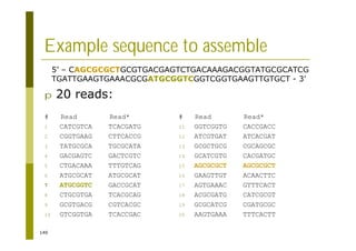
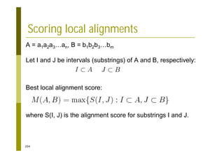
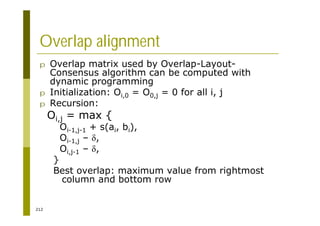
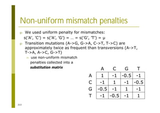
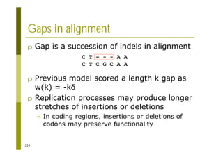
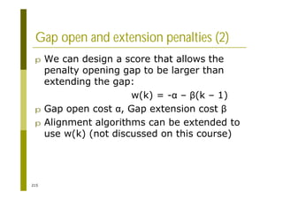
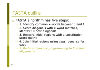
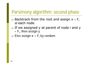
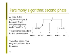
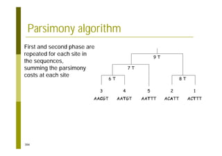
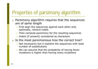
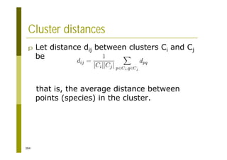
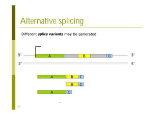
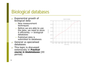
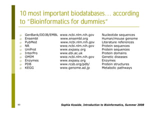
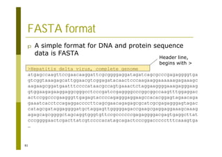
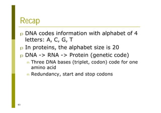
This document provides an introduction to the course "Introduction to Bioinformatics" being taught in the autumn of 2008. It discusses administrative details of the course including registration, lectures, exercises and grading. It also introduces some of the main topics that will be covered, including biological sequence analysis, genome rearrangements and phylogenetic trees. Finally, it provides information about the Master's Degree Programme in Bioinformatics and lists related bioinformatics courses offered in the Helsinki region.


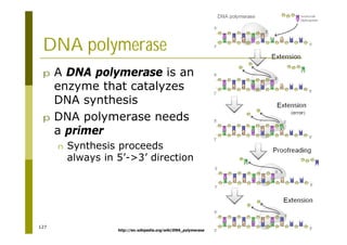
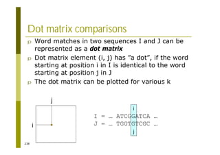
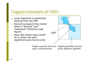
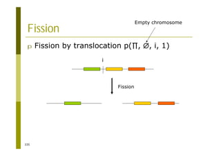
![121
#!/usr/bin/env python
import sys, random
n = int(sys.argv[1])
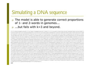
tm = {'a' : {'a' : 0.423, 'c' : 0.151, 'g' : 0.168, 't' : 0.258},
'c' : {'a' : 0.399, 'c' : 0.184, 'g' : 0.063, 't' : 0.354},
'g' : {'a' : 0.314, 'c' : 0.189, 'g' : 0.176, 't' : 0.321},
't' : {'a' : 0.258, 'c' : 0.138, 'g' : 0.187, 't' : 0.415}}
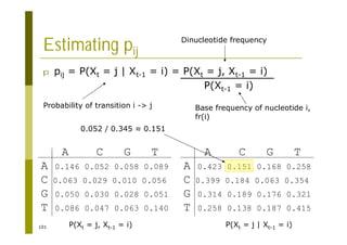
pi = {'a' : 0.345, 'c' : 0.158, 'g' : 0.159, 't' : 0.337}
def choose(dist):
r = random.random()
sum = 0.0
keys = dist.keys()
for k in keys:
sum += dist[k]
if sum > r:
return k
return keys[-1]
c = choose(pi)
for i in range(n - 1):
sys.stdout.write(c)
c = choose(tm[c])
sys.stdout.write(c)
sys.stdout.write("n")
Example Python code for generating
DNA sequences with first-order
Markov chains.
Function choose(), returns a key (here ’a’, ’c’, ’g’ or
’t’) of the dictionary ’dist’ chosen randomly
according to probabilities in dictionary values.
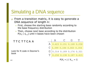
Choose the first letter, then choose
next letter according to P(xt | xt-1).
Transition matrix
tm and initial
distribution pi.
Initialisation: use packages ’sys’ and ’random’,
read sequence length from input.](https://image.slidesharecdn.com/bioinformatics-220915100249-c87e2973/85/bioinformatics-pdf-121-320.jpg)