Convergence of anaxisymmetric
finite element
François Dubois
∗
and Stefan Duprey†
1) Introduction
• Let Ω be a two-dimensional bounded domain. We suppose that its bound-
ary ∂Ω is decomposed into three components Γ0 , ΓD and ΓN:
(1.1) ∂Ω = Γ0 ∪ ΓD ∪ ΓN , Γ0 ∩ ΓD = Ø , Γ0 ∩ ΓN = Ø , ΓD ∩ ΓN = Ø,
where Γ0 is the intersection of Ω with the “axis” y = 0:
(1.2) Γ0 = Ω ∩ {(x , y) ∈ IR2
, y = 0} .
• Let f : Ω −→ IR and g : ΓN −→ IR be two given functions. We wish
to approximate the solution u of the problem
(1.3) −
∂2
u
∂x2
−
1
y
∂
∂y
y
∂u
∂y
+
u
y2
= f in Ω
(1.4) u = 0 on ΓD
(1.5)
∂u
∂n
= g on ΓN
where n is the external normal of the boundary ∂Ω.
Presented at the Fourth European Finite Element Fair, Zurich, 2-3 June
2006. Unfinished work. Edition 19 February 2008.
∗
Numerical Analysis and Partial Differential Equations, Department of
Mathematics, University Paris Sud, Bat. 425, F-91405 Orsay Cedex, EU, and
Conservatoire National des Arts et Métiers, Paris.
Mail: francois.dubois@math.u-psud.fr
† Institut de Mathématiques Elie Cartan, University Henri Poincaré, Nancy.
2.
François Dubois andStefan Duprey
• The first question is to formulate the problem (1.3)-(1.5) in order to
prove the existence and uniqueness. Our variational formulation follows the
approach of Mercier and Raugel [MR82] and is briefly recalled in Section 2.
By doing this, it is natural to introduce weighted Sobolev spaces L2
a , H1
a and
H2
a associated with axisymmetric problems. The approximation is done with
the help of finite elements. We introduce in Section 3 a simplicial conforming
mesh T composed by vertices (set T 0
), edges (set T 1
) and triangles (set
T 2
) and we denote by hT the maximal value of the Lebesgue measure of the
edges of the mesh T :
(1.6) hT = inf
a ∈ T 1
|a| .
We propose a new finite element interpolation based on vertices and defining
a discrete space H
√
T which is “naturally” associated with the Sobolev space
H1
a. The analysis of this new method is not straightforward. Due to the
singular weight y, it is necessary to use Clément’s interpolate [Cℓ75] and
Section 4 summarizes the essential of what has to be known on this subject. In
Section 5, we show that if a function u belongs to the space H2
a, it is possible
to define an interpolate ΠT u such that the error ku − ΠT uk measured with
the norm in space H1
a, is of order hT . Then the proof of convergence follows
classical arguments with Cea’s lemma (see e.g. the book [Ci78] of Ciarlet)
and is presented in Section 6.
• Some notations:
diam(K) : diameter of the triangle K.
where |•| is the bi-dimensional Lebesgue measure.
classical Sobolev spaces
space C0
(Ω).
semi-norm in Hk
(Λ) Sobolev space:
(1.7) |dk
u|2
≡
X
α+β=k
∂α+β
u
∂xα ∂yβ
2
(1.8) |u|2
k, Λ
=
Z
Λ
|dk
u|2
dx dy
2) Weighted Sobolev spaces
• We multiply the equation (1.3) by a test function v null on the portion
ΓD of the boundary and we integrate by parts relatively to the measure
y dx dy. We introduce by this calculus a bilinear form a(• , •) and a linear
form b , • according to
3.
Convergence of anaxisymmetric finite element
(2.1) a(u , v) =
Z
Ω
y ∇u • ∇v dx dy +
Z
Ω
u v
y
dx dy
(2.2) b , v =
Z
Ω
f v y dx dy +
Z
ΓN
g v y dγ .
In consequence of the algebraic expression (2.1) of the bilinear form a(•, •),
we introduce two notations. If u is some function Ω −→ IR, we define u√
and u
√
as two functions Ω −→ IR as
(2.3) u√ (x , y) =
1
√
y
u(x , y) , (x , y) ∈ Ω
(2.4) u
√
(x , y) =
√
y u(x , y) , (x , y) ∈ Ω .
• Following Mercier and Raugel [MR82], we define the three attached
Sobolev “axi-spaces”
(2.5) L2
a(Ω) = {v : Ω −→ IR , v
√
∈ L2
(Ω)}
(2.6) H1
a(Ω) = {v ∈ L2
a(Ω) , v√ ∈ L2
(Ω) , (∇v)
√
∈ (L2
(Ω))2
}
(2.7) H2
a(Ω) =
v ∈ H1
a(Ω) , v√ √ √ ∈ L2
(Ω) , (∇v)√ ∈ (L2
(Ω))2
,
(d2
v)
√
∈ (L2
(Ω))4
.
These spaces are Hilbert spaces associated with the following norms and semi-
norms defined according to:
(2.8) kvk2
0, a =
Z
Ω
y |v|2
dx dy
(2.9) |v|2
1, a =
Z
Ω
1
y
|v|2
+ y |∇v|2
dx dy
(2.10) |v|2
2, a =
Z
Ω
1
y3
|v|2
+
1
y
|∇v|2
+ y |d2
v|2
dx dy
(2.11) kvk2
1, a = kvk2
0, a + |v|2
1, a
(2.12) kvk2
2, a = kvk2
1, a + |v|2
2, a .
We do not need here the expression of the associated scalar products.
• Theorem of trace, hypotheses for f and g.
• We observe that the condition
(2.13) u = 0 on Γ0
on the axis is completely incorporated inside the choice of the axi-space
H1
a(Ω). We introduce the Sobolev space that takes into account the homoge-
neous Dirichlet boundary condition (1.4):
4.
François Dubois andStefan Duprey
(2.14) V = {v ∈ H1
a(Ω) , γv = 0 on ΓD} .
• Then the problem (1.3)-(1.5) admits the following variational formulation
(2.15)
u ∈ V
a(u , v) = b , v , ∀ v ∈ V .
Due to the fact that
(2.16) a(v , v) = |v|2
1, a , ∀ v ∈ H1
a(Ω) ,
the existence and uniqueness of the solution of problem (2.15) is easy according
to the so-called Lax-Milgram-Vishik’s lemma and we refer to [MR82] for the
study of the ellipticity property.
3) A natural axisymmetric finite element
• Let T be a conforming mesh of the domain Ω with triangles. Recall our
notations: T 0
for the set of vertices, T 1
for edges and T 2
for triangular
elements. We first observe that if we consider a function v of the form
(3.1) v(x , y) =
√
y (a x + b y + c) , (x , y) ∈ K ∈ T 2
,
we have
(3.2)
√
y ∇v(x , y) = a y ,
1
2
(a x + 3b y + c)
.
In other terms, if we denote by P1 the space of polynomials of total degree
less or equal to 1, we have:
(3.3) v√ ∈ P1 =⇒ (∇v)
√
∈ (P1)2
.
• We denote by P
√
1 the linear space
(3.5) P
√
1 = {v, v√ ∈ P1}.
We define the degrees of freedom e
δS , v for v sufficiently regular and S
vertex of the mesh T (S ∈ T 0
) by
(3.6) e
δS , v = v√ (S), S ∈ T 0
.
We observe that if the vertex S is not lying on the axis, the number
e
δS , v is nothing else that the value v(S) divided by
p
y(S). If S is on the
axis, consider this point at the origin to fix the ideas and the representation
(3.1) joined with (3.6) claims that e
δS , v = c, id est is equal to the
coefficient of
√
y that particularizes the approach. We observe that we still
have v(S) = 0 but a non trivial degree of freedom is still present for such a
vertex.
5.
Convergence of anaxisymmetric finite element
Proposition 1. Unisolvance property of the axi-finite element.
Let K ∈ T 2
be a triangle of the mesh T , Σ the set of linear forms e
δS , •
for S vertex of the triangle K (S ∈ T 0
∩ ∂K) and P
√
1 defined at relation
(3.5). Then the triple (K , Σ , P
√
1 ) that constituates our axi-finite element
is unisolvant.
Proof of Proposition 1.
Given three numbers αS ∈ IR, there exists a unique function v ∈ P
√
1 such
that
(3.7) e
δS , v = αS, S ∈ T 0
∩ ∂K .
Due to the definition of e
δS, the relation (3.7) express that v√ (S) = αS and
the hypothesis v ∈ P
√
1 express that v√ ∈ P1. Then the proof is a conse-
quence of classical arguments for linear finite elements explained e.g.in Ciar-
let’s book.
Proposition 2. Conformity of the axi-finite element.
The finite element (K , Σ , P
√
1 ) is conforming in space C0
(Ω).
Proof of Proposition 2.
The property express that given arbitrary values αS ∈ IR for all S ∈ T 0
, the
function v : Ω −→ IR defined by interpolation in each triangle K ∈ T 2
by
the relation (3.7) is lying in space C0
(Ω). The proof is nothing else that the
classical C0
−conformity of the P1 finite element: v√ ∈ P1 in each triangle
and is defined by its values in each vertex.
• We can introduce our discrete space:
(3.8) H
√
T = {v ∈ C0
(Ω), v√ |K
∈ P1, ∀ K ∈ T 2
}.
We have the property:
Proposition 3. Conformity in the axi-space H1
a(Ω).
The discrete space H
√
T is included in the axi-space H1
a(Ω) :
(3.9) H
√
T ⊂ H1
a(Ω) .
Proof of Proposition 3.
It is a direct consequence of the previous property: v ∈ H
√
T is continuous
then its gradient in the sense of distributions is a classical function. Due to
the relation (3.2), this function is clearly in the space L2
(Ω). Of course, v√
is continuous then the conditions proposed in (2.6) are all valid.
6.
François Dubois andStefan Duprey
• The discrete space for the approximation of the variational problem (2.15)
is simply
(3.10) VT = H
√
T ∩ V .
with V introduced in (2.14). The discrete variational formulation takes the
form
(3.11)
uT ∈ VT
a(uT , v) = b , v , ∀ v ∈ VT .
It has a unique solution uT ∈ VT and the question is now to estimate the
error ku − uT k measured with the norm in the axi-space H1
a(Ω). For doing
this, it is classical to study the interpolation error ku − ΠT u k when u is
sufficiently regular and ΠT u is some interpolate of function u.
4) Clément’s interpolation.
• We recall in this section the essential of what to be known about Clément’s
interpolation [Cℓ75] in the particular case of affine interpolation with triangles.
Let Ω be a bounded bidimensional domain as introduced in Section 1. Let
v be a function in space L2
(Ω). Let T be a mesh of the domain Ω and hT
introduced in (1.6). We observe also that hT is also the maximal diameter
of elements in mesh T :
(4.1) hT = sup
K∈T 2
diam(K) .
Of course, the value v(S) is not defined for a vertex S ∈ T 0
and the interest
of Clément’s interpolate is to introduce such an approached value even if v
only belongs to the space L2
(Ω).
• First, if S ∈ ΓD, we set
(4.2) δC
S , v = 0 , S ∈ T 0
∩ ΓD .
If not, for S ∈ T 0
, we introduce the subset ΞS of Ω defined by
(4.3) ΞS =
[
K∈T 2, ∂K⊃S
K
and presented on Figure 1. The interpolate value δC
S , v at the vertex S
is defined by
(4.4) δC
S , v =
1
|ΞS|
Z
ΞS
v(x) dx dy , S ∈ T 0
, S /
∈ ΓD .
• First we introduce the Clement interpolate ΠC
v of v ∈ L2
(Ω) with the
help of classical P1 continuous interpolate functions ϕS defined by
7.
Convergence of anaxisymmetric finite element
(4.5) ϕS|K
∈ P1 , ∀ K ∈ T 2
, ϕS(S′
) =
1 if S′
= S
0 if S′
6= S .
With Clément [Cℓ75], we set
(4.6) ΠC
v =
X
S∈T 0
δC
S , v ϕS .
S
K
Figure 1. Left: Vicinity ΞS of the vertex S ∈ T 0
.
Right: Vicinity ZK for a given triangle K ∈ T 2
.
• We suppose now that the function v is a bit more regular. The interest of
Clément’s interpolation is that all the Ciarlet-Raviart [CR72] classical results
for Lagrange interpolation in Sobolev spaces can be extented to Clément’s.
In order to quantify the result, we suppose in the following that the mesh T
belongs to a family F of meshes such that no infinitesimal angle belongs in
the mesh T ; in other terms,
(4.7) ∃ C 0 , ∀ T ∈ F , ∀ S ∈ T 0
, ♯{K ∈ T 2
, K ⊂ ΞS} ≤ C .
We introduce also the set ZK for a given triangle K ∈ T 2
(see again the
Figure 1) :
(4.8) ZK = {L ∈ T 2
, K ∩ L 6= Ø} =
[
S∈T 0, S⊂∂K
ΞS .
According to the hypothesis (4.7), we have
(4.9) ∃ C 0 , ∀ T ∈ F , ∀ K ∈ T 2
, ♯ZK ≤ C .
• Consider now a function v ∈ H1
(ZK). Then a main results of Clément’s
contribution can be stated as
8.
François Dubois andStefan Duprey
(4.10) |v − ΠC
v|0, K
≤ C hT |v|1, ZK
(4.11) |v − ΠC
v|1, K
≤ C |v|1, ZK
with a constant C 0 that does not depend on the particular mesh T
chosen in the family F. If the function v is more regular (v ∈ H2
(ZK )), we
can consolidate the estimate (4.11):
(4.12) |v − ΠC
v|1, K
≤ C hT |v|2, ZK
.
Finally, if v is globally regular, we have
(4.13) kv − ΠC
vk0, Ω
≤ C hT |v|1, Ω
.
5) An interpolation result
• We suppose in this section that a given function u belongs to the space
H2
a(Ω) defined in (2.7). It is possible to define the value u(S) for a vertex
S ∈ T 0
due to the Sobolev embedding Theorem (see e.g. Brézis [Br83]) that
claims that
(5.1) H2
(Ω) ⊂ C0
(Ω) .
The question is now to define or not the number e
δS , u introduced in
(3.6).
Proposition 4. Lack of regularity.
Let u ∈ H2
a(Ω) and u√ introduced in (2.3). Then u√ belongs to the space
H1
(Ω) and we have
(5.2) ku√ k1, Ω ≤ C kuk2, a
Proof of Proposition 4.
We set
(5.3) v ≡ u√
and we have the following calculus:
(5.4) ∇v = −
1
2y
√
y
u ∇y +
1
√
y
∇u .
Then
Z
Ω
|v|2
dx dy ≤
Z
Ω
1
y
|u|2
dx dy ≤ C kuk2
2, a
Z
Ω
|∇v|2
dx dy ≤ 2
Z
Ω
1
4y3
|u|2
+
1
y
|∇u|2
dx dy ≤ C kuk2
2, a .
Due to (2.10), the relation (5.2) is established.
9.
Convergence of anaxisymmetric finite element
• Il we derive (formally !) the relation (5.4), we get
(5.5) d2
v =
3
4 y2√
y
u ∇y • ∇y −
1
y
√
y
∇u • ∇y +
1
√
y
d2
u
and we have not sufficiently powers of y to be sure that we obtain a finite
result when we integrate the square of d2
v. In consequence, the function v is
not necessarily continuous. Nevertheless, it is possible to define the Clement
interpolate of u√ relatively to the mesh T and due to (5.2), this interpolate
has good regularity properties. We define our interpolate Πu by conjugation
and we set
(5.6) Πu = ΠC
u√
√
or equivalently
(5.7) Πu(x, y) =
√
y ΠC
v
(x, y) , (x, y) ∈ K ∈ T 2
with v(•) introduced in (5.3).
• We assume that the mesh T admits angles that are aware from 0 and π :
(5.8)
(
∃ (α , β) , 0 α
π
2
β π , ∀ T ∈ F , ∀ K ∈ T 2
,
∀ θ angle in K , α ≤ θ ≤ β.
We observe that the hypothesis (5.8) clearly implies (4.7). We assume also
that the sizes of triangles are quasi-uniform:
(5.9) ∃ γ 0 , ∀ T ∈ F , ∀ a ∈ T 1
, γ hT ≤ |a| ≤ hT
with hT introduced at the relation (1.6). We have the following interpolation
theorem:
Theorem 1. An interpolation result.
We suppose that the mesh T belongs to a family F that satisfy the above
hypotheses (5.8) and (5.9). Let u ∈ H2
a(Ω) and Πu defined by (5.6). Then
we have
(5.10) ku − Πuk1, a ≤ C hT kuk2, a .
• In order to prepare the technical points of the proof, we introduce, fol-
lowing [MR82] the sub-domains Ω+ and Ω− as
(5.12) Ω+ = {K ∈ T 2
, dist (ZK , Γ0) 0}
(5.13) Ω− = Ω Ω+ .
10.
François Dubois andStefan Duprey
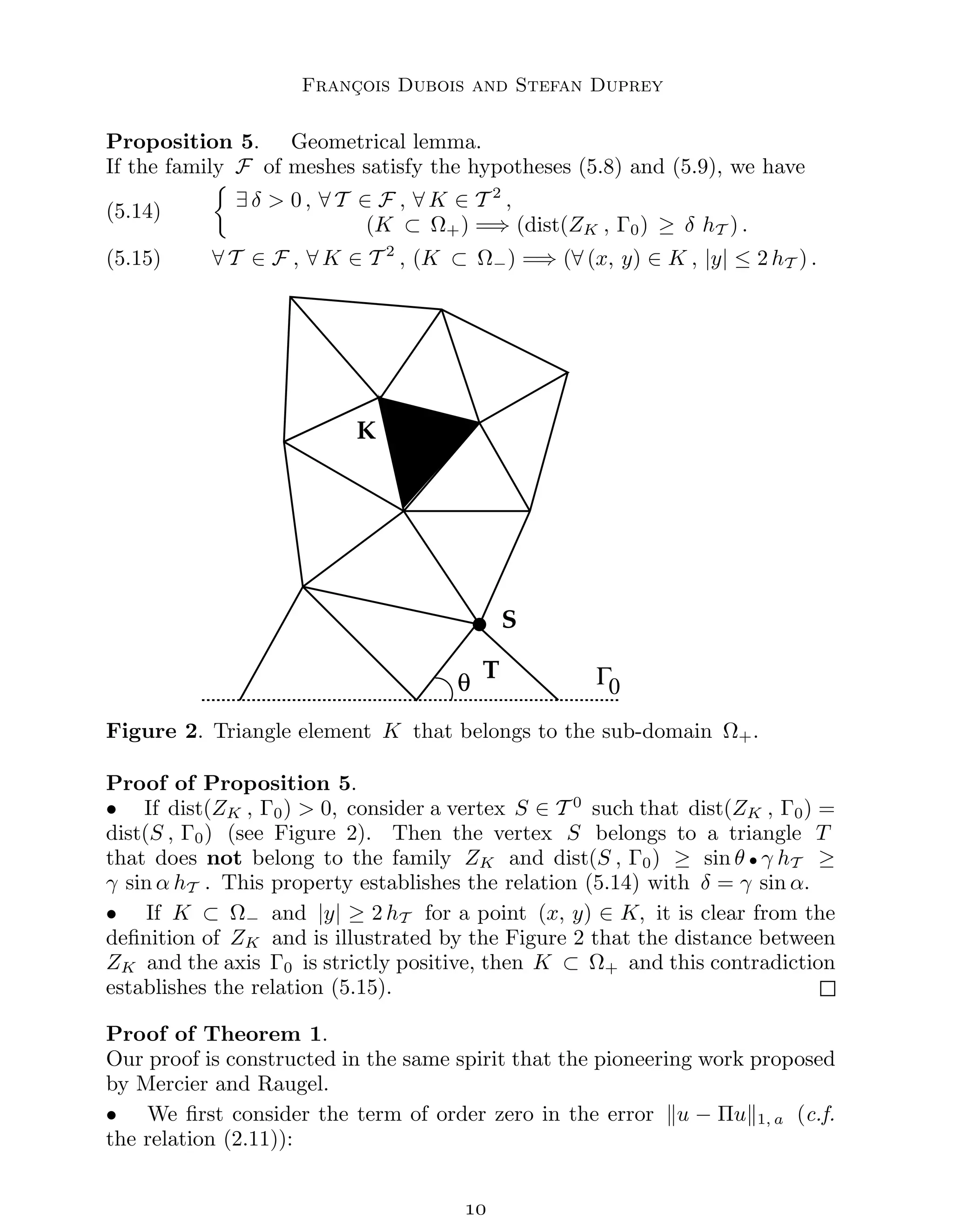
Proposition 5. Geometrical lemma.
If the family F of meshes satisfy the hypotheses (5.8) and (5.9), we have
(5.14)
∃ δ 0 , ∀ T ∈ F , ∀ K ∈ T 2
,
(K ⊂ Ω+) =⇒ (dist(ZK , Γ0) ≥ δ hT ) .
(5.15) ∀ T ∈ F , ∀ K ∈ T 2
, (K ⊂ Ω−) =⇒ (∀ (x, y) ∈ K , |y| ≤ 2 hT ) .
S
0
Γ
T
θ
K
Figure 2. Triangle element K that belongs to the sub-domain Ω+.
Proof of Proposition 5.
• If dist(ZK , Γ0) 0, consider a vertex S ∈ T 0
such that dist(ZK , Γ0) =
dist(S , Γ0) (see Figure 2). Then the vertex S belongs to a triangle T
that does not belong to the family ZK and dist(S , Γ0) ≥ sin θ • γ hT ≥
γ sin α hT . This property establishes the relation (5.14) with δ = γ sin α.
• If K ⊂ Ω− and |y| ≥ 2 hT for a point (x, y) ∈ K, it is clear from the
definition of ZK and is illustrated by the Figure 2 that the distance between
ZK and the axis Γ0 is strictly positive, then K ⊂ Ω+ and this contradiction
establishes the relation (5.15).
Proof of Theorem 1.
Our proof is constructed in the same spirit that the pioneering work proposed
by Mercier and Raugel.
• We first consider the term of order zero in the error ku − Πuk1, a (c.f.
the relation (2.11)):
11.
Convergence of anaxisymmetric finite element
Z
Ω
1
y
|u − Πu|2
dx dy =
Z
Ω
1
y
|u −
√
y ΠC
v|2
dx dy
=
Z
Ω
|v − ΠC
v|2
dx dy = kv − ΠC
vk2
0, Ω
≤ C h2
T |v|2
1, Ω due to (4.13)
≤ C h2
T kvk2
2, a according to (5.2)
(5.16)
Z
Ω
1
y
|u − Πu|2
dx dy = kv − ΠC
vk2
0, Ω ≤ C h2
T kuk2
2, a .
• On the other hand, we have
∇
√
y v − ΠC
v
=
1
2
√
y
v − ΠC
v
∇y +
√
y ∇ v − ΠC
v
.
Then
(5.17)
Z
Ω
y |∇ u − Πu
|2
dx dy ≤
≤
Z
Ω
|v − ΠC
v|2
dx dy + 2
Z
Ω
y2
|∇ v − ΠC
v
|2
dx dy .
The first term in the right hand side of (5.17) is majored with the help of
estimation (5.16). We focus now on the second term. We have
Z
Ω
y2
|∇(v − ΠC
v)|2
dx dy =
=
Z
Ω+
y2
∇(|v − ΠC
v)|2
dx dy +
Z
Ω−
y2
|∇(v − ΠC
v)|2
dx dy .
• From the relation (5.16), we have for the internal sub-domain Ω− :
Z
Ω−
y2
|∇(v − ΠC
v)|2
dx dy ≤ 4 h2
T
Z
Ω−
|∇ v − Πv
|2
dx dy
≤ C h2
T |v|2
1, Ω due to (4.11)
≤ C h2
T kuk2
2, a thanks to (5.2)
(5.18)
Z
Ω−
y |∇(v − ΠC
v)|2
dx dy ≤ C h2
T kuk2
2, a .
• We have in the external part of the domain
Z
Ω+
y2
|∇(v − ΠC
v)|2
dx dy =
X
K∈T 2, K⊂Ω+
Z
K
y2
|∇(v − ΠC
v)|2
dx dy .
We fix K ⊂ Ω+, we introduce (ymin , ymax) according to
ymin = min
(x, y)∈K
y , ymax = max
(x, y)∈K
y .
12.
François Dubois andStefan Duprey
Then ymin ≤ y ≤ ymax, ymax − ymin ≤ hT and
(5.19) y2
≤ y2
max ≤ 2 y2
min + h2
T
, (x , y) ∈ K .
Now if (x , y) ∈ ZK, we have, due to the definition of ZK and to (5.15):
ymin − hT ≤ y , y ≥ δ hT
and
(5.20)
y2
min + h2
T
y2
≤
1
y2
(2 y2
+ 2 h2
T + h2
T ) ≤ 2 +
3
δ2
.
• Due to the property (4.12) of Clément’s interpolate and to estimate (5.20),
we have
Z
K
y2
|∇(v − ΠC
v)|2
dx dy ≤ 2 (y2
min + h2
T )
Z
K
|∇(v − ΠC
v)|2
dx dy
≤ 2 (y2
min + h2
T )
Z
ZK
C h2
T |d2
v|2
dx dy
≤ C
2 +
3
δ2
h2
T
Z
ZK
y2
|d2
v|2
dx dy
≤ C h2
T
Z
ZK
1
y3
|v|2
+
1
y
|∇v|2
+ y |d2
v|2
dx dy
according to (5.5). Then, taking into account (2.10), we have
(5.22)
Z
Ω+
y2
|∇(v − ΠC
v)|2
dx dy ≤ C h2
T kuk2
2, a .
The inequality (5.11) is a consequence of (5.16), (5.17), (5.18) and (5.22). The
theorem is now established.
6) Convergence of the axi-finite element approximation.
• We suppose now that the data Ω, f and g are chosen in such a way that
the solution u of the variational problem (2.13) belongs to the space H2
a(Ω) :
(6.1) u ∈ H2
a(Ω) , u solution of problem (2.13).
Let uT ∈ H
√
T be the solution of the discrete problem (3.11).
Theorem 2. First order approximation
Under the above hypotheses, we have
(6.2) ku − uT k1, a ≤ C hT kuk2, a .
13.
Convergence of anaxisymmetric finite element
Proof of Theorem 2.
It is a classical consequence of the ellipticity of the functional a(• , •) and of
Céa’s lemma. We denote by κ the ellipticity constant of the functional. Thus
we get
κ ku − uT k2
1, a ≤ a(u − uT , u − uT )
≤ C a(u − uT , u − Πu) take v = Πu − uT ∈ H
√
T in (3.11)
≤ C ku − uT k1, a ku − ΠuT k1, a .
Then ku − uT k1, a ≤ C ku − Πuk1, a ≤ C hT kuk2, a
due to the theorem 1.
7) References.
[Br85] H. Brézis. Analyse fonctionnelle. Théorie et applications, Masson,
Paris, 1983.
[CR72] P.G. Ciarlet, P.A. Raviart. “General Lagrange and Hermite inter-
polation in IRn
with applications to finite element methods”, Archive for
Rational Mechanics and Analysis, vol. 46, p. 177-199, 1972.
[Ci78] P.G. Ciarlet. The Finite Element Method for Elliptic Problems, Se-
ries “Studies in Mathematics and its Applications”, North-Holland, Am-
sterdam, 1978.
[Cℓ75] P. Clément. “Approximation by finite element functions using local
regularization”, R.A.I.R.O Analyse numérique, vol. 9, no
2, p. 77-84,
1975.
[DD06] F. Dubois, S.Duprey. “Eléments finis naturels pour l’axisymétrique”,
reseauch report, may 2006.
[MR82] B. Mercier, G. Raugel. “Résolution d’un problème aux limites dans
un ouvert axisymétrique par éléments finis en (r, z) et séries de Fourier
en θ”, R.A.I.R.O Analyse numérique, vol. 16, no
4, p. 405-461, 1982.
![François Dubois and Stefan Duprey
• The first question is to formulate the problem (1.3)-(1.5) in order to
prove the existence and uniqueness. Our variational formulation follows the
approach of Mercier and Raugel [MR82] and is briefly recalled in Section 2.
By doing this, it is natural to introduce weighted Sobolev spaces L2
a , H1
a and
H2
a associated with axisymmetric problems. The approximation is done with
the help of finite elements. We introduce in Section 3 a simplicial conforming
mesh T composed by vertices (set T 0
), edges (set T 1
) and triangles (set
T 2
) and we denote by hT the maximal value of the Lebesgue measure of the
edges of the mesh T :
(1.6) hT = inf
a ∈ T 1
|a| .
We propose a new finite element interpolation based on vertices and defining
a discrete space H
√
T which is “naturally” associated with the Sobolev space
H1
a. The analysis of this new method is not straightforward. Due to the
singular weight y, it is necessary to use Clément’s interpolate [Cℓ75] and
Section 4 summarizes the essential of what has to be known on this subject. In
Section 5, we show that if a function u belongs to the space H2
a, it is possible
to define an interpolate ΠT u such that the error ku − ΠT uk measured with
the norm in space H1
a, is of order hT . Then the proof of convergence follows
classical arguments with Cea’s lemma (see e.g. the book [Ci78] of Ciarlet)
and is presented in Section 6.
• Some notations:
diam(K) : diameter of the triangle K.
where |•| is the bi-dimensional Lebesgue measure.
classical Sobolev spaces
space C0
(Ω).
semi-norm in Hk
(Λ) Sobolev space:
(1.7) |dk
u|2
≡
X
α+β=k
∂α+β
u
∂xα ∂yβ
2
(1.8) |u|2
k, Λ
=
Z
Λ
|dk
u|2
dx dy
2) Weighted Sobolev spaces
• We multiply the equation (1.3) by a test function v null on the portion
ΓD of the boundary and we integrate by parts relatively to the measure
y dx dy. We introduce by this calculus a bilinear form a(• , •) and a linear
form b , • according to
](https://image.slidesharecdn.com/dubois-duprey-2008-axi-element-250618162520-aa6f82a4/75/Axisymmetric-finite-element-convergence-results-2-2048.jpg)
![Convergence of an axisymmetric finite element
(2.1) a(u , v) =
Z
Ω
y ∇u • ∇v dx dy +
Z
Ω
u v
y
dx dy
(2.2) b , v =
Z
Ω
f v y dx dy +
Z
ΓN
g v y dγ .
In consequence of the algebraic expression (2.1) of the bilinear form a(•, •),
we introduce two notations. If u is some function Ω −→ IR, we define u√
and u
√
as two functions Ω −→ IR as
(2.3) u√ (x , y) =
1
√
y
u(x , y) , (x , y) ∈ Ω
(2.4) u
√
(x , y) =
√
y u(x , y) , (x , y) ∈ Ω .
• Following Mercier and Raugel [MR82], we define the three attached
Sobolev “axi-spaces”
(2.5) L2
a(Ω) = {v : Ω −→ IR , v
√
∈ L2
(Ω)}
(2.6) H1
a(Ω) = {v ∈ L2
a(Ω) , v√ ∈ L2
(Ω) , (∇v)
√
∈ (L2
(Ω))2
}
(2.7) H2
a(Ω) =
v ∈ H1
a(Ω) , v√ √ √ ∈ L2
(Ω) , (∇v)√ ∈ (L2
(Ω))2
,
(d2
v)
√
∈ (L2
(Ω))4
.
These spaces are Hilbert spaces associated with the following norms and semi-
norms defined according to:
(2.8) kvk2
0, a =
Z
Ω
y |v|2
dx dy
(2.9) |v|2
1, a =
Z
Ω
1
y
|v|2
+ y |∇v|2
dx dy
(2.10) |v|2
2, a =
Z
Ω
1
y3
|v|2
+
1
y
|∇v|2
+ y |d2
v|2
dx dy
(2.11) kvk2
1, a = kvk2
0, a + |v|2
1, a
(2.12) kvk2
2, a = kvk2
1, a + |v|2
2, a .
We do not need here the expression of the associated scalar products.
• Theorem of trace, hypotheses for f and g.
• We observe that the condition
(2.13) u = 0 on Γ0
on the axis is completely incorporated inside the choice of the axi-space
H1
a(Ω). We introduce the Sobolev space that takes into account the homoge-
neous Dirichlet boundary condition (1.4):
](https://image.slidesharecdn.com/dubois-duprey-2008-axi-element-250618162520-aa6f82a4/75/Axisymmetric-finite-element-convergence-results-3-2048.jpg)
![François Dubois and Stefan Duprey
(2.14) V = {v ∈ H1
a(Ω) , γv = 0 on ΓD} .
• Then the problem (1.3)-(1.5) admits the following variational formulation
(2.15)
u ∈ V
a(u , v) = b , v , ∀ v ∈ V .
Due to the fact that
(2.16) a(v , v) = |v|2
1, a , ∀ v ∈ H1
a(Ω) ,
the existence and uniqueness of the solution of problem (2.15) is easy according
to the so-called Lax-Milgram-Vishik’s lemma and we refer to [MR82] for the
study of the ellipticity property.
3) A natural axisymmetric finite element
• Let T be a conforming mesh of the domain Ω with triangles. Recall our
notations: T 0
for the set of vertices, T 1
for edges and T 2
for triangular
elements. We first observe that if we consider a function v of the form
(3.1) v(x , y) =
√
y (a x + b y + c) , (x , y) ∈ K ∈ T 2
,
we have
(3.2)
√
y ∇v(x , y) = a y ,
1
2
(a x + 3b y + c)
.
In other terms, if we denote by P1 the space of polynomials of total degree
less or equal to 1, we have:
(3.3) v√ ∈ P1 =⇒ (∇v)
√
∈ (P1)2
.
• We denote by P
√
1 the linear space
(3.5) P
√
1 = {v, v√ ∈ P1}.
We define the degrees of freedom e
δS , v for v sufficiently regular and S
vertex of the mesh T (S ∈ T 0
) by
(3.6) e
δS , v = v√ (S), S ∈ T 0
.
We observe that if the vertex S is not lying on the axis, the number
e
δS , v is nothing else that the value v(S) divided by
p
y(S). If S is on the
axis, consider this point at the origin to fix the ideas and the representation
(3.1) joined with (3.6) claims that e
δS , v = c, id est is equal to the
coefficient of
√
y that particularizes the approach. We observe that we still
have v(S) = 0 but a non trivial degree of freedom is still present for such a
vertex.
](https://image.slidesharecdn.com/dubois-duprey-2008-axi-element-250618162520-aa6f82a4/75/Axisymmetric-finite-element-convergence-results-4-2048.jpg)
![François Dubois and Stefan Duprey
• The discrete space for the approximation of the variational problem (2.15)
is simply
(3.10) VT = H
√
T ∩ V .
with V introduced in (2.14). The discrete variational formulation takes the
form
(3.11)
uT ∈ VT
a(uT , v) = b , v , ∀ v ∈ VT .
It has a unique solution uT ∈ VT and the question is now to estimate the
error ku − uT k measured with the norm in the axi-space H1
a(Ω). For doing
this, it is classical to study the interpolation error ku − ΠT u k when u is
sufficiently regular and ΠT u is some interpolate of function u.
4) Clément’s interpolation.
• We recall in this section the essential of what to be known about Clément’s
interpolation [Cℓ75] in the particular case of affine interpolation with triangles.
Let Ω be a bounded bidimensional domain as introduced in Section 1. Let
v be a function in space L2
(Ω). Let T be a mesh of the domain Ω and hT
introduced in (1.6). We observe also that hT is also the maximal diameter
of elements in mesh T :
(4.1) hT = sup
K∈T 2
diam(K) .
Of course, the value v(S) is not defined for a vertex S ∈ T 0
and the interest
of Clément’s interpolate is to introduce such an approached value even if v
only belongs to the space L2
(Ω).
• First, if S ∈ ΓD, we set
(4.2) δC
S , v = 0 , S ∈ T 0
∩ ΓD .
If not, for S ∈ T 0
, we introduce the subset ΞS of Ω defined by
(4.3) ΞS =
[
K∈T 2, ∂K⊃S
K
and presented on Figure 1. The interpolate value δC
S , v at the vertex S
is defined by
(4.4) δC
S , v =
1
|ΞS|
Z
ΞS
v(x) dx dy , S ∈ T 0
, S /
∈ ΓD .
• First we introduce the Clement interpolate ΠC
v of v ∈ L2
(Ω) with the
help of classical P1 continuous interpolate functions ϕS defined by
](https://image.slidesharecdn.com/dubois-duprey-2008-axi-element-250618162520-aa6f82a4/75/Axisymmetric-finite-element-convergence-results-6-2048.jpg)
![Convergence of an axisymmetric finite element
(4.5) ϕS|K
∈ P1 , ∀ K ∈ T 2
, ϕS(S′
) =
1 if S′
= S
0 if S′
6= S .
With Clément [Cℓ75], we set
(4.6) ΠC
v =
X
S∈T 0
δC
S , v ϕS .
S
K
Figure 1. Left: Vicinity ΞS of the vertex S ∈ T 0
.
Right: Vicinity ZK for a given triangle K ∈ T 2
.
• We suppose now that the function v is a bit more regular. The interest of
Clément’s interpolation is that all the Ciarlet-Raviart [CR72] classical results
for Lagrange interpolation in Sobolev spaces can be extented to Clément’s.
In order to quantify the result, we suppose in the following that the mesh T
belongs to a family F of meshes such that no infinitesimal angle belongs in
the mesh T ; in other terms,
(4.7) ∃ C 0 , ∀ T ∈ F , ∀ S ∈ T 0
, ♯{K ∈ T 2
, K ⊂ ΞS} ≤ C .
We introduce also the set ZK for a given triangle K ∈ T 2
(see again the
Figure 1) :
(4.8) ZK = {L ∈ T 2
, K ∩ L 6= Ø} =
[
S∈T 0, S⊂∂K
ΞS .
According to the hypothesis (4.7), we have
(4.9) ∃ C 0 , ∀ T ∈ F , ∀ K ∈ T 2
, ♯ZK ≤ C .
• Consider now a function v ∈ H1
(ZK). Then a main results of Clément’s
contribution can be stated as
](https://image.slidesharecdn.com/dubois-duprey-2008-axi-element-250618162520-aa6f82a4/75/Axisymmetric-finite-element-convergence-results-7-2048.jpg)
![François Dubois and Stefan Duprey
(4.10) |v − ΠC
v|0, K
≤ C hT |v|1, ZK
(4.11) |v − ΠC
v|1, K
≤ C |v|1, ZK
with a constant C 0 that does not depend on the particular mesh T
chosen in the family F. If the function v is more regular (v ∈ H2
(ZK )), we
can consolidate the estimate (4.11):
(4.12) |v − ΠC
v|1, K
≤ C hT |v|2, ZK
.
Finally, if v is globally regular, we have
(4.13) kv − ΠC
vk0, Ω
≤ C hT |v|1, Ω
.
5) An interpolation result
• We suppose in this section that a given function u belongs to the space
H2
a(Ω) defined in (2.7). It is possible to define the value u(S) for a vertex
S ∈ T 0
due to the Sobolev embedding Theorem (see e.g. Brézis [Br83]) that
claims that
(5.1) H2
(Ω) ⊂ C0
(Ω) .
The question is now to define or not the number e
δS , u introduced in
(3.6).
Proposition 4. Lack of regularity.
Let u ∈ H2
a(Ω) and u√ introduced in (2.3). Then u√ belongs to the space
H1
(Ω) and we have
(5.2) ku√ k1, Ω ≤ C kuk2, a
Proof of Proposition 4.
We set
(5.3) v ≡ u√
and we have the following calculus:
(5.4) ∇v = −
1
2y
√
y
u ∇y +
1
√
y
∇u .
Then
Z
Ω
|v|2
dx dy ≤
Z
Ω
1
y
|u|2
dx dy ≤ C kuk2
2, a
Z
Ω
|∇v|2
dx dy ≤ 2
Z
Ω
1
4y3
|u|2
+
1
y
|∇u|2
dx dy ≤ C kuk2
2, a .
Due to (2.10), the relation (5.2) is established.
](https://image.slidesharecdn.com/dubois-duprey-2008-axi-element-250618162520-aa6f82a4/75/Axisymmetric-finite-element-convergence-results-8-2048.jpg)
![Convergence of an axisymmetric finite element
• Il we derive (formally !) the relation (5.4), we get
(5.5) d2
v =
3
4 y2√
y
u ∇y • ∇y −
1
y
√
y
∇u • ∇y +
1
√
y
d2
u
and we have not sufficiently powers of y to be sure that we obtain a finite
result when we integrate the square of d2
v. In consequence, the function v is
not necessarily continuous. Nevertheless, it is possible to define the Clement
interpolate of u√ relatively to the mesh T and due to (5.2), this interpolate
has good regularity properties. We define our interpolate Πu by conjugation
and we set
(5.6) Πu = ΠC
u√
√
or equivalently
(5.7) Πu(x, y) =
√
y ΠC
v
(x, y) , (x, y) ∈ K ∈ T 2
with v(•) introduced in (5.3).
• We assume that the mesh T admits angles that are aware from 0 and π :
(5.8)
(
∃ (α , β) , 0 α
π
2
β π , ∀ T ∈ F , ∀ K ∈ T 2
,
∀ θ angle in K , α ≤ θ ≤ β.
We observe that the hypothesis (5.8) clearly implies (4.7). We assume also
that the sizes of triangles are quasi-uniform:
(5.9) ∃ γ 0 , ∀ T ∈ F , ∀ a ∈ T 1
, γ hT ≤ |a| ≤ hT
with hT introduced at the relation (1.6). We have the following interpolation
theorem:
Theorem 1. An interpolation result.
We suppose that the mesh T belongs to a family F that satisfy the above
hypotheses (5.8) and (5.9). Let u ∈ H2
a(Ω) and Πu defined by (5.6). Then
we have
(5.10) ku − Πuk1, a ≤ C hT kuk2, a .
• In order to prepare the technical points of the proof, we introduce, fol-
lowing [MR82] the sub-domains Ω+ and Ω− as
(5.12) Ω+ = {K ∈ T 2
, dist (ZK , Γ0) 0}
(5.13) Ω− = Ω Ω+ .
](https://image.slidesharecdn.com/dubois-duprey-2008-axi-element-250618162520-aa6f82a4/75/Axisymmetric-finite-element-convergence-results-9-2048.jpg)
![Convergence of an axisymmetric finite element
Proof of Theorem 2.
It is a classical consequence of the ellipticity of the functional a(• , •) and of
Céa’s lemma. We denote by κ the ellipticity constant of the functional. Thus
we get
κ ku − uT k2
1, a ≤ a(u − uT , u − uT )
≤ C a(u − uT , u − Πu) take v = Πu − uT ∈ H
√
T in (3.11)
≤ C ku − uT k1, a ku − ΠuT k1, a .
Then ku − uT k1, a ≤ C ku − Πuk1, a ≤ C hT kuk2, a
due to the theorem 1.
7) References.
[Br85] H. Brézis. Analyse fonctionnelle. Théorie et applications, Masson,
Paris, 1983.
[CR72] P.G. Ciarlet, P.A. Raviart. “General Lagrange and Hermite inter-
polation in IRn
with applications to finite element methods”, Archive for
Rational Mechanics and Analysis, vol. 46, p. 177-199, 1972.
[Ci78] P.G. Ciarlet. The Finite Element Method for Elliptic Problems, Se-
ries “Studies in Mathematics and its Applications”, North-Holland, Am-
sterdam, 1978.
[Cℓ75] P. Clément. “Approximation by finite element functions using local
regularization”, R.A.I.R.O Analyse numérique, vol. 9, no
2, p. 77-84,
1975.
[DD06] F. Dubois, S.Duprey. “Eléments finis naturels pour l’axisymétrique”,
reseauch report, may 2006.
[MR82] B. Mercier, G. Raugel. “Résolution d’un problème aux limites dans
un ouvert axisymétrique par éléments finis en (r, z) et séries de Fourier
en θ”, R.A.I.R.O Analyse numérique, vol. 16, no
4, p. 405-461, 1982.
](https://image.slidesharecdn.com/dubois-duprey-2008-axi-element-250618162520-aa6f82a4/75/Axisymmetric-finite-element-convergence-results-13-2048.jpg)


![[DSC Europe 25] Nikola Rajovic - Hardware Technologies Under the Hood: RISC-V...](https://cdn.slidesharecdn.com/ss_thumbnails/o2gptrmtoyqndgoshwgq-dsc2025-tenstorrent-rajovic-251205090438-814685f5-thumbnail.jpg?width=640&height=640&fit=bounds)
![[DSC Europe 25] Vid Stimac - Policy Parsimony: Between Oversimplifying and Ov...](https://cdn.slidesharecdn.com/ss_thumbnails/eqlepagzqp2rhg3gbluh-dsc-stimac-251120-251205090438-059e7f54-thumbnail.jpg?width=640&height=640&fit=bounds)

![[DSC Europe 25] Boris Perkovic - Lost in performance.pptx](https://cdn.slidesharecdn.com/ss_thumbnails/uq5hrp7vsuahqkxzifux-1-251204082258-fd2ee09d-thumbnail.jpg?width=640&height=640&fit=bounds)


