This document is a thesis presented to Reed College that analyzes business models in the music industry in the digital age. It provides background on the traditional music industry structure, which was dominated by major record labels that signed artists and funded the production and promotion of albums. With the rise of the internet and digital music in the 2000s, barriers to entry for artists have decreased and new models have emerged that allow artists more control over their profits across music products and concerts. The thesis aims to empirically test hypotheses about how free streaming, paid downloads, and concert attendance may be related for profit-maximizing artists.


![2.2. File-Sharing and Music Industry Profits 15
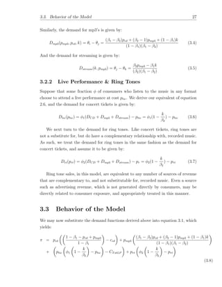
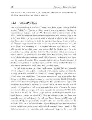
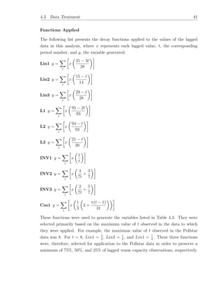
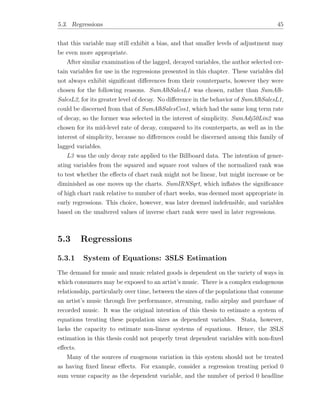
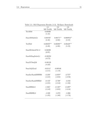
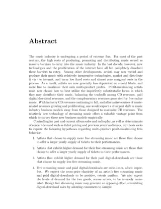
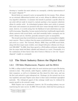
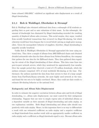
sumers’ demand for recorded media. Consumers may purchase a given recording for
price pr or may obtain an illegal copy for free. These consumers are indexed by
x 2 [0, +1], according to a declining preference for obtaining the given recording,
and their utility functions are given by:
max{↵(1 x) + N pr, (1 x) + N, 0}, (2.1)
where the first term is consumers’ utility from consuming a purchased recording, the
second from consuming an illegal copy, and the third from choosing not to consume.
↵ and are parameters for consumers’ utilities from obtaining the paid and illegal
copies of the recording. N is the total number of consumers in possession of the
recording, regardless of whether their copies are legal or illegal. The parameter
reflects the extent to which the potential utility from obtaining the recording increases
with N. Hence, this parameter represents the additional utility that results from a
network e↵ect as the recording becoming more popular. The authors assume that
legally and illegally-obtained recordings are vertically di↵erentiated such that ↵ >
> . The implication of this assumption is that, given that the set of all consumers
is continuously distributed along a number line, this continuum is partitioned into
three segments at two points, which represent two marginal consumers. One of these
consumers is indi↵erent between purchasing or downloading the recording and the
other is indi↵erent between downloading the recording or not obtaining it at all.
Hence, the set of all consumers is partitioned such that, if one imagines the continuum
of all consumers vertically, its upper segment contains all consumers who purchase
the recording, its middle segment contains all consumers who illegally download the
recording, and its bottom segment contains all consumers who do not obtain the
recording.
The authors then proceed to assume that live performance has a linear demand
function, though they note that they do so only for the sake of simplicity. This
demand is given by qp = max{ N pp, 0}, where, pp is the ticket price and the
parameter ( > 0) measures the extent to which the magnitude of N a↵ects live
performance demand. Next, the authors assume that musical artists price concert
tickets as monopolists, bear no costs and maximize their live performance profit
function, ⇡p = ppqp = pp( N pp). Ticket price and profits from live performance are
therefore given by:
pp =
N
2
) ⇡p = p2
p =
2
N2
4
(2.2)
Next the authors note that N is the single determinant of the location of the](https://image.slidesharecdn.com/f58d7578-f631-4fa4-b017-f660b0284b8b-160413083921/85/AndrewShapiro-SeniorThesis-ReedCollege-21-320.jpg)

![2.2. File-Sharing and Music Industry Profits 17
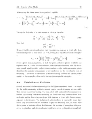
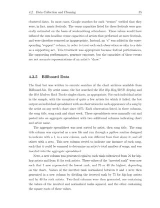
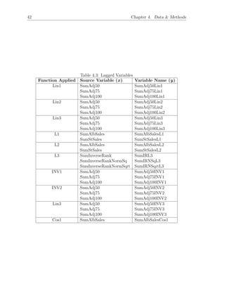
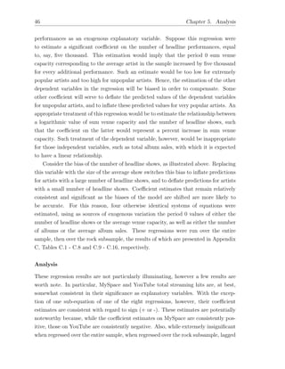
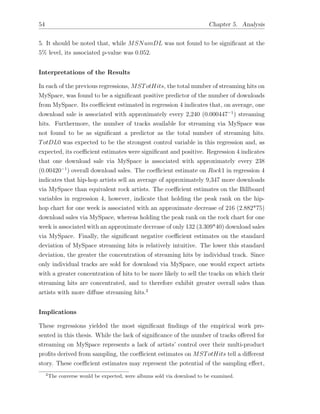
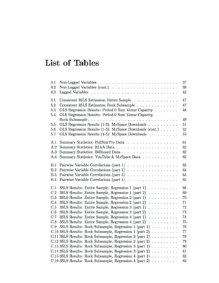
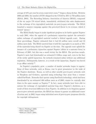
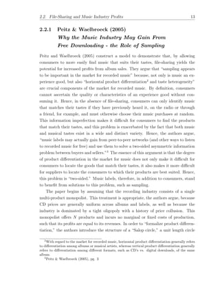
2.2.3 Grassi (2007)
The Music Market in the Age of Download
Grassi (2007) closely parallels the work of Gayer & Shy (2006), though the variations
between the two papers are of great significance. Grassi begins by examining empirical
data from the Italian markets for music and home video. He discerns market trends
not only concurrent with increasing levels of file-sharing and internet access, but also
market trends concurrent with shifts in the dominant media format, such as those
that occurred with the emergence of the CD as the dominant format. He notes that
such shifts allow firms to increase their profits, since some consumers will repurchase
the same product in a new media format, which he refers to as a “replacement e↵ect.”
Grassi places consumers in essentially the same theoretical framework as that
of Gayer & Shy, however, the mathematical construction of his model is notably
di↵erent. Like Gayer & Shy, he assumes that the demand for music comes from a
uniformly distributed continuum of consumers. His indexation of these consumers
by ✓, however, is far more intuitive. Placing ✓ 2 [0, 1] and introducing one recording
available for purchase price p, which is set by a monopolist, consumers’ utility is given
U = max{✓ p, 0}. Grassi then introduces a pirated imperfect substitute good, the
utility from which is discounted by the factor , and which costs consumers some price
w, such that U = max{✓ p, ✓ w, 0}. The parameter w essentially represents the
opportunity cost of illegal downloading as presented in Peitz & Waelbroek (2005),
however, Grassi notes that a component of this opportunity cost is fear of litigation.
This model omits the network e↵ect on album sales presented by Gayer & Shy (2005),
which was N in their model. Also, where Gayer & Shy constructed a strict inequality,
Grassi explores the “corner solutions,” such as values of that annihilate the market
for legally purchased music.
Grassi also explores a number of extensions of Gayer & Shy’s model. He places the
sampling e↵ect in a simple, two-period, inter-temporal framework, for example. The
crucial aspect of this framework is the introduction of the parameter as the factor
by which the demand for illegal downloads in period one increases the demand for
CD’s in the following period, where clearly 0 < < 1. The model can be manipulated
to show that, for w = 0, record label profits are not diminished by file-sharing if and
only if 2 . File-sharing, therefore, inevitably diminishes record label profits if
the quality of pirate copies is greater than half that of CD’s. Grassi also extends the
model to include paid download sales of a digital-format good. This good is sold for
price q, by the same firm that sells the CD, and yields utility discounted by the factor](https://image.slidesharecdn.com/f58d7578-f631-4fa4-b017-f660b0284b8b-160413083921/85/AndrewShapiro-SeniorThesis-ReedCollege-23-320.jpg)

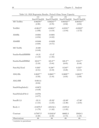
![2.2. File-Sharing and Music Industry Profits 19
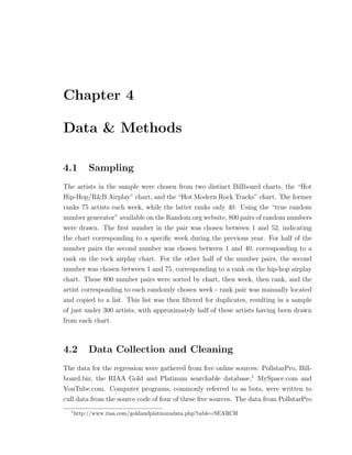
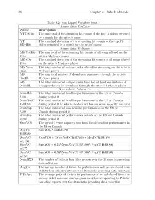
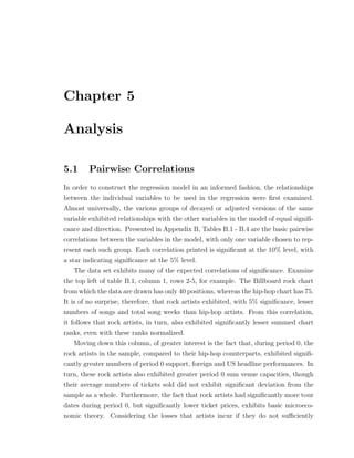
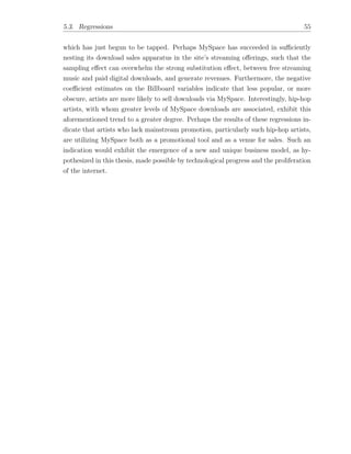
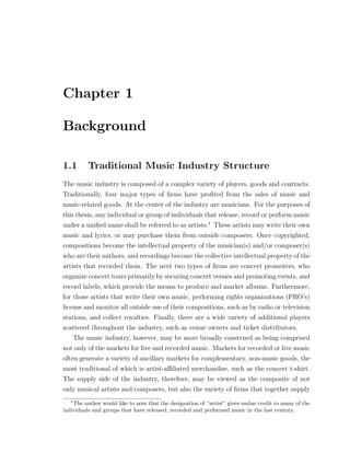
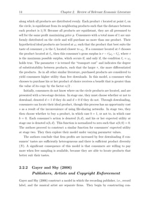
availability of free digital copies of their recordings.
In the case of streaming music, pirated copies of most recordings are available
for streaming via YouTube. Via myspace, however, one may stream o cial copies
of recordings, though only those chosen at the artist’s discretion, which unlike pi-
rated copies are guaranteed to be full quality, properly labeled, and easily searchable.
artists, therefore, may decrease consumers’ opportunity costs from searching and mis-
labels, as well as potentially increase the average quality of their free streaming music
available online, and, therefore, diminish w
by o↵ering a larger proportion of their
catalog on MySpace. In accordance with Grassi’s model, this should increase live
performance revenues and overall profits for most artists, but diminish CD revenues
and record label profits.
Returning to his introduction, though Grassi discusses the topics of the “replace-
ment e↵ect” and shifts in dominant media formats only briefly and in passing, further
discussion of these topics is warranted. In the final paragraph of his paper, Grassi
comments that “industries that sold the machines used by the pirates have increased
their business, and for example the market of the MP3 players [sic] has been invented
from nothing. Probably the ‘big enemy’ of the recording industry is not the final
consumers, that occasionally can act as a pirate [sic], but the industries that are
cannibalizing music market profits.”4
Inferences
It appears that the major US record labels failed to anticipate the shift in dominant
format from CDs to mp3s. It is logical that the RIAA observed such a strong cor-
relation between CD sales displacement and piracy via Napster because, as the first
major source of pirated digital media, Napster served as an excellent proxy for the un-
observed shift in dominant formats. Clearly, if labels had not begun to o↵er music in
newer formats as vinyl or cassette tapes grew obsolete, they would have experienced
a similar sales displacement. Furthermore, physical media formats can deteriorate
over time, losing quality or breaking entirely. Not only do such phenomena increase
potential profits from the replacement e↵ect, but they will no longer occur with new
digital formats. The advent of digital media was an opportunity for record labels
to increase their profits, however, they failed to capitalize on the replacement e↵ect.
Furthermore, they allowed the Apple corporation to dominate the emerging market
and gradually absorb their target consumers: music purchasers.
4
Grassi (2007), pg. 23](https://image.slidesharecdn.com/f58d7578-f631-4fa4-b017-f660b0284b8b-160413083921/85/AndrewShapiro-SeniorThesis-ReedCollege-25-320.jpg)

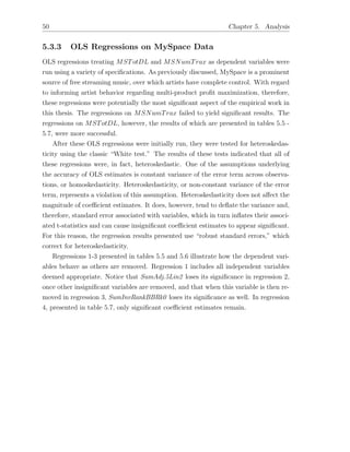
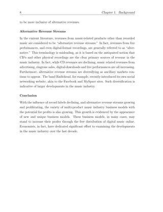
![24 Chapter 3. Theory
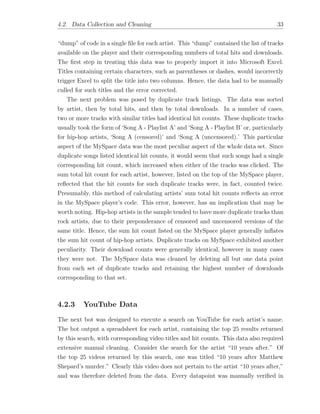
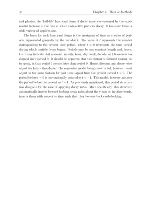
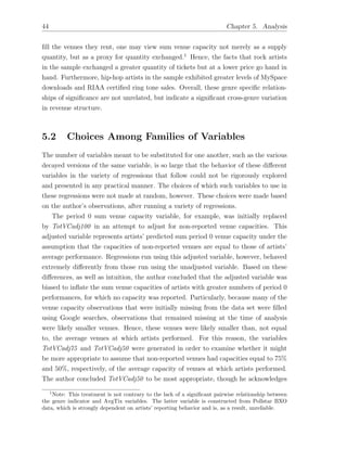
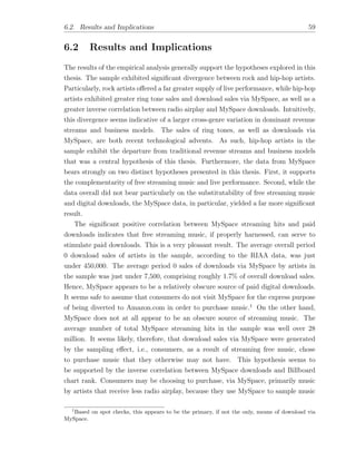
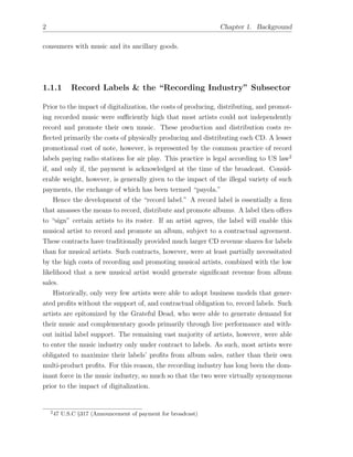
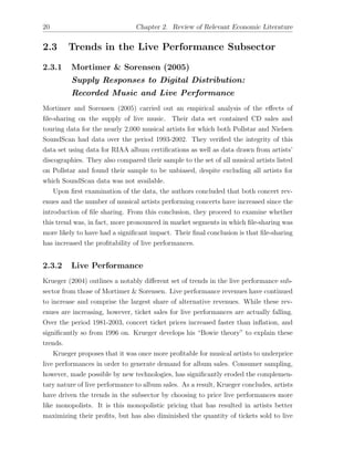
3.2 Demand Functions
At this point, we return to the work of Grassi (2007) in order to derive the demand
functions on which the artist profit function is dependent. Assume that an artist has
one album of recorded music, which is made available to consumers in hardcopy CD,
downloadable mp3, and streaming formats. The demand for these goods comes from
a continuum of consumers with a uniform distribution, which is illustrated below.
This distribution is indexed by ✓ 2 [0, 1], according to a decreasing preference for
consumption.
3.2.1 Consumers
Suppose that every consumer in the world were given the CD for free, and each gave
a completely accurate rating of his or her enjoyment of the CD on a scale from zero
to one. Suppose the consumers were then placed in a line facing left (towards 0), such
that every consumer rated the CD more highly than the consumer behind him or her.
This would be a (discrete) representation of a continuum of consumers indexed by
✓ 2 [0, 1] according to decreasing preference. Each consumer represents a point on
the continuum. The value of ✓ corresponding to this point is equal to this consumer’s
rating of the CD. Now, ✓ indexes a “uniform distribution.” The implications of this
uniformity, returning to the image of the world’s consumers in a line (facing right),
are that the rating of the CD by the first consumer in line is 1, and of the last is
0. Furthermore, as one proceeds down the line from each consumer to the next,
the corresponding ratings decrease by a constant amount. In other words, no matter
which consumer one chooses to examine, the di↵erence between this consumer’s rating
and that of the consumer in front of him or her, will be the same.
Consumer Utility
Introducing all three goods and their associated prices and costs, we adapt equation
2.5 to the notation of this theory section. Hence, consumers’ utility is given by the
maximum value of:
UMAX(✓ pcd, 1✓ pmp3, 2✓ k, 0) (3.2)
where the first term represents the potential utility from consumption of the CD, the
second from consumption of the mp3, the third from streaming consumption of the
album, and the final from non-consumption.
Clearly pcd and pmp3 denote the price of the CD and the mp3, respectively. Hence,](https://image.slidesharecdn.com/f58d7578-f631-4fa4-b017-f660b0284b8b-160413083921/85/AndrewShapiro-SeniorThesis-ReedCollege-29-320.jpg)