DAA

1. Analysis of Algorithms 1
Analysis of Algorithms
• Running Time
• Pseudo-Code
• Analysis of
Algorithms
• Asymptotic Notation
• Asymptotic Analysis
• Mathematical facts
n = 4
Algorithm
Input
T(n)
Output

2. Analysis of Algorithms 2
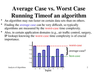
Average Case vs. Worst Case
Running Timeof an algorithm
• An algorithm may run faster on certain data sets than on others.
• Finding the average case can be very difficult, so typically
algorithms are measured by the worst-case time complexity.
• Also, in certain application domains (e.g., air traffic control, surgery,
IP lookup) knowing the worst-case time complexity is of crucial
importance.
Input
1 ms
2 ms
3 ms
4 ms
5 ms
A B C D E F G
worst-case
best-case
}average-case?

3. Analysis of Algorithms 3
Measuring the Running Time
• How should we measure the running time of an algorithm?
• Approach 1: Experimental Study
– Write a program that implements the algorithm
– Run the program with data sets of varying size and composition.
– Use a method like System.currentTimeMillis() to get an accurate
measure of the actual running time.
50 100
0
t (ms)
n
10
20
30
40
50
60

4. Analysis of Algorithms 4
Beyond Experimental Studies
• Experimental studies have several limitations:
– It is necessary to implement and test the algorithm in order to
determine its running time.
– Experiments can be done only on a limited set of inputs, and may not
be indicative of the running time on other inputs not included in the
experiment.
– In order to compare two algorithms, the same hardware and software
environments should be used.

5. Analysis of Algorithms 5
Beyond Experimental Studies
• We will now develop a general methodology for
analyzing the running time of algorithms. In
contrast to the "experimental approach", this
methodology:
– Uses a high-level description of the algorithm instead of
testing one of its implementations.
– Takes into account all possible inputs.
– Allows one to evaluate the efficiency of any algorithm in a
way that is independent from the hardware and software
environment.

6. Analysis of Algorithms 6
Pseudo-Code
• Pseudo-code is a description of an algorithm that is more structured
than usual prose but less formal than a programming language.
• Example: finding the maximum element of an array.
Algorithm arrayMax(A, n):
Input: An array A storing n integers.
Output: The maximum element in A.
currentMax  A[0]
for i 1 to n -1 do
if currentMax < A[i] then currentMax  A[i]
return currentMax
• Pseudo-code is our preferred notation for describing algorithms.
• However, pseudo-code hides program design issues.

7. Analysis of Algorithms 7
What is Pseudo-Code ?
• A mixture of natural language and high-level programming concepts that
describes the main ideas behind a generic implementation of a data structure or
algorithm.
-Expressions: use standard mathematical symbols to describe numeric and
boolean expressions -use  for assignment (“=” in Java)
-use = for the equality relationship (“==” in Java)
-Method Declarations: -Algorithm name(param1, param2)
-Programming Constructs: - decision structures: if ... then ... [else ... ]
- while-loops: while ... do
- repeat-loops: repeat ... until ...
- for-loop: for ... do
- array indexing: A[i]
-Methods: - calls: object method(args)
- returns: return value

8. 8
Analysis of Algorithms
• Primitive Operations: Low-level computations
independent from the programming language can be
identified in pseudocode.
• Examples:
– calling a method and returning from a method
– arithmetic operations (e.g. addition)
– comparing two numbers, etc.
• By inspecting the pseudo-code, we can count the number
of primitive operations executed by an algorithm.

9. Analysis of Algorithms 9
Example:
Algorithm arrayMax(A, n):
Input: An array A storing n integers.
Output: The maximum element in A.
currentMax ¨ A[0]
for i ¨ 1 to n -1 do
if currentMax < A[i] then
currentMax  A[i]
return currentMax

10. Analysis of Algorithms 10
Asymptotic Notation
• Goal: to simplify analysis by getting rid of
unneeded information (like “rounding”
1,000,001≈1,000,000)
• We want to say in a formal way 3n2
≈ n2
• The “Big-Oh” Notation:
– given functions f(n) and g(n), we say that f(n)
is O(g(n) ) if and only if there are positive
constants c and n0 such that f(n)≤ c g(n) for n
≥ n0

11. Analysis of Algorithms 11
Example
g(n) = n
c g(n) = 4n
n
f(n) = 2n + 6
For functions f(n)
and g(n) (to the
right) there are
positive constants c
and n0 such that:
f(n)≤c g(n) for n ≥
n0
conclusion:
2n+6 is O(n).

12. Analysis of Algorithms 12
Another Example
On the other hand…
n2
is not O(n) because there is
no c and n0 such that:
n2
≤ cn for n ≥ n0
(As the graph to the right
illustrates, no matter how large
a c is chosen there is an n big
enough that n2
>cn ) .

13. Analysis of Algorithms 13
Asymptotic Notation (cont.)
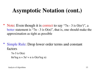
• Note: Even though it is correct to say “7n - 3 is O(n3
)”, a
better statement is “7n - 3 is O(n)”, that is, one should make the
approximation as tight as possible
• Simple Rule: Drop lower order terms and constant
factors
7n-3 is O(n)
8n2
log n + 5n2
+ n is O(n2
log n)

14. Analysis of Algorithms 14
Asymptotic Notation
(terminology)
• Special classes of algorithms:
logarithmic: O(log n)
linear: O(n)
quadratic: O(n2
)
polynomial: O(nk
), k ≥ 1
exponential: O(an
), n > 1
• “Relatives” of the Big-Oh
  (f(n)): Big Omega--asymptotic lower bound
  (f(n)): Big Theta--asymptotic tight bound

15. 15
Asymptotic Analysis of The
Running Time
• Use the Big-Oh notation to express the number of primitive
operations executed as a function of the input size.
• For example, we say that the arrayMax algorithm runs in O(n)
time.
• Comparing the asymptotic running time
-an algorithm that runs in O(n) time is better than one that runs in O(n2
) time
-similarly, O(log n) is better than O(n)
-hierarchy of functions: log n << n << n2
<< n3
<< 2n
• Caution! Beware of very large constant factors. An algorithm
running in time 1,000,000 n is still O(n) but might be less efficient
on your data set than one running in time 2n2
, which is O(n2
)

16. 16
Example of Asymptotic
Analysis
An algorithm for computing prefix averages
Algorithm prefixAverages1(X):
Input: An n-element array X of numbers.
Output: An n -element array A of numbers such that A[i] is the average of elements
X[0], ... , X[i].
Let A be an array of n numbers.
for i 0 to n - 1 do
a  0
for j  0 to i do
a  a + X[j]
A[i]  a/(i+ 1)
return array A
• Analysis ...
1 step i iterations
with
i=0,1,2...n-1
n iterations

17. Analysis of Algorithms 17
Another Example
• A better algorithm for computing prefix averages:
Algorithm prefixAverages2(X):
Input: An n-element array X of numbers.
Output: An n -element array A of numbers such that A[i] is the average of
elements X[0], ... , X[i].
Let A be an array of n numbers.
s 0
for i  0 to n do
s  s + X[i]
A[i]  s/(i+ 1)
return array A
• Analysis ...

18. Analysis of Algorithms 18
Math You Need to Review
Logarithms and Exponents (Appendix A, p.617)
• properties of logarithms:
logb(xy) = logbx + logby
logb (x/y) = logbx - logby
logbxa = alogbx
logba= logxa/logxb
• properties of exponentials:
a(b+c)
= ab
a c
abc
= (ab
)c
ab
/ac
= a(b-c)
b = a log
a
b
bc
= a c*log
a
b

19. Analysis of Algorithms 19
More Math to Review
• Floor:x = the largest integer ≤ x
• Ceiling: x = the smallest integer ≥ x
• Summations: (see Appendix A, p.619)
• Geometric progression: (see Appendix A, p.620)