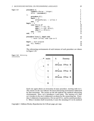
This document provides an overview of the topics that will be covered in the book. It discusses different programming paradigms that will be examined, including imperative, functional, object-oriented, dataflow, concurrent, declarative, and aggregate languages. For each paradigm, examples of relevant languages are given and the chapters where those languages will be discussed are indicated. The goal is to study principles and innovations across a wide range of modern programming languages. Formal semantic models that provide precise definitions of language meaning will also be presented.
![xiii
at in the text are developed more thoroughly in this latter type of exercise.
In order to create an appearance of uniformity, I have chosen to modify the
syntax of presented languages (in cases where the syntax is not the crucial is-
sue), so that language-specific syntax does not obscure the other points that I
am trying to make. For examples that do not depend on any particular lan-
guage, I have invented what I hope will be clear notation. It is derived
largely from Ada and some of its predecessors. This notation allows me to
standardize the syntactic form of language, so that the syntax does not ob-
scure the subject at hand. It is largely irrelevant whether a particular lan-
guage uses begin and end or { and } . On the other hand, in those cases
where I delve deeply into a language in current use (like ML, LISP, Prolog,
Smalltalk, and C++), I have preserved the actual language. Where reserved
words appear, I have placed them in bold monospace. Other program ex-
cerpts are in monospace font. I have also numbered examples so that instruc-
tors can refer to parts of them by line number. Each technical term that is
introduced in the text is printed in boldface the first time it appears. All
boldface entries are collected and defined in the glossary. I have tried to use a
consistent nomenclature throughout the book.
In order to relieve the formality common in textbooks, I have chosen to
write this book as a conversation between me, in the first singular person,
and you, in the second person. When I say we, I mean you and me together. I
hope you don’t mind.
Several supplemental items are available to assist the instructor in using
this text. Answers to the exercises are available from the publisher (ISBN:
0-201-49835-9) in a disk-based format. The figures from the text (in Adobe
Acrobat format), an Adobe Acrobat reader, and the entire text of this book are
available from the following site:
ftp://aw.com/cseng/authors/finkel
Please check the readme file for updates and changes. The complete text of
this book is intended for on-screen viewing free of charge; use of this material
in any other format is subject to a fee.
There are other good books on programming language design. I can par-
ticularly recommend the text by Pratt [Pratt 96] for elementary material and
the text by Louden [Louden 93] for advanced material. Other good books in-
clude those by Sebesta [Sebesta 93] and Sethi [Sethi 89].
I owe a debt of gratitude to the many people who helped me write this
book. Much of the underlying text is modified from course notes written by
Charles N. Fischer of the University of Wisconsin–Madison. Students in my
classes have submitted papers which I have used in preparing examples and
text; these include the following:
Copyright Addison-Wesley. Reproduction fee $.02 per page, per copy.
PREFACE](https://image.slidesharecdn.com/advancedprogramminglanguagedesign-230706034617-464d64c2/85/Advanced_programming_language_design-pdf-7-320.jpg)
![3
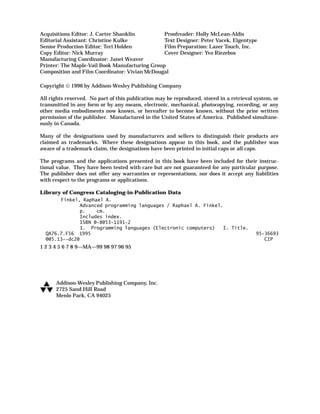
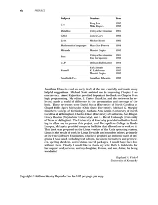
1. What is the structure (syntax) and meaning (semantics) of the program-
ming language constructs? Usually, I will use informal methods to show
what the constructs are and what they do. However, Chapter 10 pre-
sents formal methods for describing the semantics of programming lan-
guages.
2. How does the compiler writer deal with these constructs in order to
translate them into assembler or machine language? The subject of
compiler construction is large and fascinating, but is beyond the scope of
this book. I will occasionally touch on this topic to assure you that the
constructs can, in fact, be translated.
3. Is the programming language good for the programmer? More specifi-
cally, is it easy to use, expressive, readable? Does it protect the pro-
grammer from programming errors? Is it elegant? I spend a significant
amount of effort trying to evaluate programming languages and their
constructs in this way. This subject is both fascinating and difficult to
be objective about. Many languages have their own fan clubs, and dis-
cussions often revolve about an ill-defined sense of elegance.
Programming languages have a profound effect on the ways programmers
formulate solutions to problems. You will see that different paradigms im-
pose very different programming styles, but even more important, they
change the way the programmer looks at algorithms. I hope that this book
will expand your horizons in much the same way that your first exposure to
recursion opened up a new way of thinking. People have invented an amaz-
ing collection of elegant and expressive programming structures.
2 ◆ EVALUATING PROGRAMMING LANGUAGES
This book introduces you to some unusual languages and some unusual lan-
guage features. As you read about them, you might wonder how to evaluate
the quality of a feature or an entire language. Reasonable people disagree on
what makes for a great language, which is why so many novel ideas abound
in the arena of programming language design. At the risk of oversimplifica-
tion, I would like to present a short list of desiderata for programming lan-
guages [Butcher 91]. Feel free to disagree with them. Another excellent
discussion of this topic is found in Louden [Louden 93].
• Simplicity. There should be as few basic concepts as possible. Often the
job of the language designer is to discard elements that are superfluous,
error-prone, hard to read, or hard to compile. Many people consider PL/I,
for example, to be much too large a language. Some criticize Ada for the
same reason.
• Uniformity. The basic concepts should be applied consistently and uni-
versally. We should be able to use language features in different contexts
without changing their form. Non-uniformity can be annoying. In Pascal,
constants cannot be declared with values given by expressions, even
though expressions are accepted in all other contexts when a value is
needed. Non-uniformity can also be error-prone. In Pascal, some for
loops take a single statement as a body, but repeat loops can take any
number of statements. It is easy to forget to bracket multiple statements
in the body of a for loop.
Copyright Addison-Wesley. Reproduction fee $.02 per page, per copy.
2 EVALUATING PROGRAMMING LANGUAGES](https://image.slidesharecdn.com/advancedprogramminglanguagedesign-230706034617-464d64c2/85/Advanced_programming_language_design-pdf-11-320.jpg)
![• Orthogonality. Independent functions should be controlled by indepen-
dent mechanisms. (In mathematics, independent vectors are called ‘‘or-
thogonal.’’)
• Abstraction. There should be a way to factor out recurring patterns.
(Abstraction generally means hiding details by constructing a ‘‘box’’
around them and permitting only limited inspection of its contents.)
• Clarity. Mechanisms should be well defined, and the outcome of code
should be easily predictable. People should be able to read programs in
the language and be able to understand them readily. Many people have
criticized C, for example, for the common confusion between the assign-
ment operator (=) and the equality test operator (==).
• Information hiding. Program units should have access only to the in-
formation they require. It is hard to write large programs without some
control over the extent to which one part of the program can influence an-
other part.
• Modularity. Interfaces between programming units should be stated ex-
plicitly.
• Safety. Semantic errors should be detectable, preferably at compile time.
An attempt to add values of dissimilar types usually indicates that the
programmer is confused. Languages like Awk and SNOBOL that silently
convert data types in order to apply operators tend to be error-prone.
• Expressiveness. A wide variety of programs should be expressible.1
Languages with coroutines, for example, can express algorithms for test-
ing complex structures for equality much better than languages without
coroutines. (Coroutines are discussed in Chapter 2.)
• Efficiency. Efficient code should be producible from the language, possi-
bly with the assistance of the programmer. Functional programming lan-
guages that rely heavily on recursion face the danger of inefficiency,
although there are compilation methods (such as eliminating tail recur-
sion) that make such languages perfectly acceptable. However, languages
that require interpretation instead of compilation (such as Tcl) tend to be
slow, although in many applications, speed is of minor concern.
3 ◆ BACKGROUND MATERIAL ON
PROGRAMMING LANGUAGES
Before showing you anything out of the ordinary, I want to make sure that
you are acquainted with the fundamental concepts that are covered in an un-
dergraduate course in programming languages. This section is intentionally
concise. If you need more details, you might profitably refer to the fine books
by Pratt [Pratt 96] and Louden [Louden 93].
hhhhhhhhhhhhhhhhhhhhhhhhhhhhhhhhhhhh
1
In a formal sense, all practical languages are Turing-complete; that is, they can express
exactly the same algorithms. However, the ease with which a programmer can come up with an
appropriate program is part of what I mean by expressiveness. Enumerating binary trees (see
Chapter 2) is quite difficult in most languages, but quite easy in CLU.
Copyright Addison-Wesley. Reproduction fee $.02 per page, per copy.
4 CHAPTER 1 INTRODUCTION](https://image.slidesharecdn.com/advancedprogramminglanguagedesign-230706034617-464d64c2/85/Advanced_programming_language_design-pdf-12-320.jpg)
![5
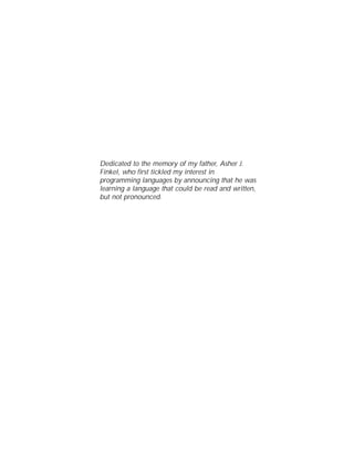
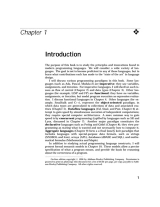
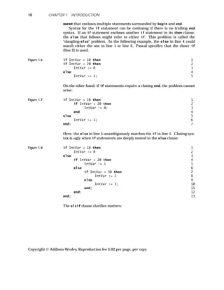
3.1 Variables, Data Types, Literals, and
Expressions
I will repeatedly refer to the following example, which is designed to have a
little bit of everything in the way of types. A type is a set of values on which
the same operations are defined.
Figure 1.2 variable 1
First : pointer to integer; 2
Second : array 0..9 of 3
record 4
Third: character; 5
Fourth: integer; 6
Fifth : (Apple, Durian, Coconut, Sapodilla, 7
Mangosteen) 8
end; 9
begin 10
First := nil; 11
First := &Second[1].Fourth; 12
Firstˆ := 4; 13
Second[3].Fourth := (Firstˆ + Second[1].Fourth) * 14
Second[Firstˆ].Fourth; 15
Second[0] := [Third : ’x’; Fourth : 0; 16
Fifth : Sapodilla]; 17
end; 18
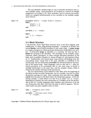
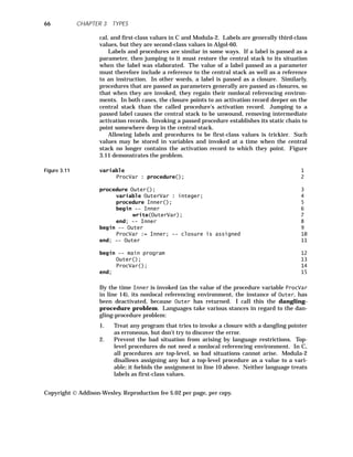
Imperative languages (such as Pascal and Ada) have variables, which are
named memory locations. Figure 1.2 introduces two variables, First (line 2)
and Second (lines 3–9). Programming languages often restrict the values that
may be placed in variables, both to ensure that compilers can generate accu-
rate code for manipulating those values and to prevent common programming
errors. The restrictions are generally in the form of type information. The
type of a variable is a restriction on the values it can hold and what opera-
tions may be applied to those values. For example, the type integer encom-
passes numeric whole-number values between some language-dependent (or
implementation-dependent) minimum and maximum value; values of this
type may act as operands in arithmetic operations such as addition. The
term integer is not set in bold monospace type, because in most languages,
predefined types are not reserved words, but ordinary identifiers that can be
given new meanings (although that is bad practice).
Researchers have developed various taxonomies to categorize types
[ISO/IEC 94; Meek 94]. I will present here a fairly simple taxonomy. A
primitive type is one that is not built out of other types. Standard primitive
types provided by most languages include integer, Boolean, character, real,
and sometimes string. Figure 1.2 uses both integer and character. Enu-
meration types are also primitive. The example uses an enumeration type in
lines 7–8; its values are restricted to the values specified. Enumeration types
often define the order of their enumeration constants. In Figure 1.2, however,
Copyright Addison-Wesley. Reproduction fee $.02 per page, per copy.
3 BACKGROUND MATERIAL ON PROGRAMMING LANGUAGES](https://image.slidesharecdn.com/advancedprogramminglanguagedesign-230706034617-464d64c2/85/Advanced_programming_language_design-pdf-13-320.jpg)
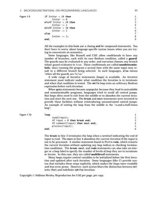
![it makes no sense to consider one fruit greater than another.2
Structured types are built out of other types. Arrays, records, and
pointers are structured types.3
Figure 1.2 shows all three kinds of standard
structured types. The building blocks of a structured type are its compo-
nents. The component types go into making the structured type; component
values go into making the value of a structured type. The pointer type in line
2 of Figure 1.2 has one component type (integer); a pointer value has one
component value. There are ten component values of the array type in lines
3–9, each of a record type. Arrays are usually required to be homogeneous;
that is, all the component values must be of the same type. Arrays are in-
dexed by elements of an index type, usually either a subrange of integers,
characters, or an enumeration type. Therefore, an array has two component
types (the base type and the index type); it has as many component values as
there are members in the index type.
Flexible arrays do not have declared bounds; the bounds are set at run-
time, based on which elements of the array have been assigned values. Dy-
namic-sized arrays have declared bounds, but the bounds depend on the
runtime value of the bounds expressions. Languages that provide dynamic-
sized arrays provide syntax for discovering the lower and upper bounds in
each dimension.
Array slices, such as Second[3..5], are also components for purposes of
this discussion. Languages (like Ada) that allow array slices usually only al-
low slices in the last dimension. (APL does not have such a restriction.)
The components of the record type in lines 4–9 are of types character and
integer. Records are like arrays in that they have multiple component val-
ues. However, the values are indexed not by members of an index type but
rather by named fields. The component values need not be of the same type;
records are not required to be homogeneous. Languages for systems pro-
gramming sometimes allow the programmer to control exactly how many bits
are allocated to each field and how fields are packed into memory.
The choice is a less common structured type. It is like a record in that it
has component types, each selected by a field. However, it has only one com-
ponent value, which corresponds to exactly one of the component types.
Choices are often implemented by allocating as much space as the largest
component type needs. Some languages (like Simula) let the programmer re-
strict a variable to a particular component when the variable is declared. In
this case, only enough space is allocated for that component, and the compiler
disallows accesses to other components.
Which field is active in a choice value determines the operations that may
be applied to that value. There is usually some way for a program to deter-
mine at runtime which field is active in any value of the choice type; if not,
there is a danger that a value will be accidentally (or intentionally) treated as
belonging to a different field, which may have a different type. Often, lan-
guages provide a tagcase statement with branches in which the particular
variant is known both to the program and to the compiler. Pascal allows part
hhhhhhhhhhhhhhhhhhhhhhhhhhhhhhhhhhhh
2
In Southeast Asia, the durian is considered the king of fruits. My personal favorite is the
mangosteen.
3
Whether to call pointers primitive or structured is debatable. I choose to call them struc-
tured because they are built from another type.
Copyright Addison-Wesley. Reproduction fee $.02 per page, per copy.
6 CHAPTER 1 INTRODUCTION](https://image.slidesharecdn.com/advancedprogramminglanguagedesign-230706034617-464d64c2/85/Advanced_programming_language_design-pdf-14-320.jpg)
![9
Figure 1.3 type 1
FirstType = ... ; 2
SecondType = ... ; 3
SecondTypePtr = pointer to SecondType; 4
variable 5
F : FirstType; 6
S : SecondType; 7
begin 8
... 9
S := F qua SecondType; -- Wisconsin Modula 10
S := (SecondTypePtr(&F))ˆ; -- C 11
end; 12
Line 10 shows how F can be cast without conversion into the second type in
Wisconsin Modula. Line 11 shows the same thing for C, where I use the type
name SecondTypePtr as an explicit conversion routine. The referencing oper-
ator & produces a pointer to F. In both cases, if the two types disagree on
length of representation, chaos may ensue, because the number of bytes
copied by the assignment is the appropriate number for SecondType.
The Boolean operators and and or may have short-circuit semantics;
that is, the second operand is only evaluated if the first operand evaluates to
true (for and) or false (for or). This evaluation strategy is an example of
lazy evaluation, discussed in Chapter 4. Short-circuit operators allow the
programmer to combine tests, the second of which only makes sense if the
first succeeds. For example, I may want to first test if a pointer is nil, and
only if it is not, to test the value it points to.
Conditional expressions are built with an if construct. To make sure
that a conditional expression always has a value, each if must be matched by
both a then and an else. The expressions in the then and else parts must
have the same type. Here is an example:
Figure 1.4 write(if a > 0 then a else -a);
3.2 Control Constructs
Execution of imperative programming languages proceeds one statement at
a time. Statements can be simple or compound. Simple statements include
the assignment statement, procedure invocation, and goto. Compound state-
ments enclose other statements; they include conditional and iterative state-
ments, such as if, case, while, and for. Programming languages need some
syntax for delimiting enclosed statements in a compound statement. Some
languages, like Modula, provide closing syntax for each compound statement:
Figure 1.5 while Firstˆ < 10 do 1
Firstˆ := 2 * Firstˆ; 2
Second[0].Fourth := 1 + Second[0].Fourth; 3
end; 4
The end on line 4 closes the while on line 1. Other languages, like Pascal,
only allow a single statement to be included, but it may be a block state-
Copyright Addison-Wesley. Reproduction fee $.02 per page, per copy.
3 BACKGROUND MATERIAL ON PROGRAMMING LANGUAGES](https://image.slidesharecdn.com/advancedprogramminglanguagedesign-230706034617-464d64c2/85/Advanced_programming_language_design-pdf-17-320.jpg)
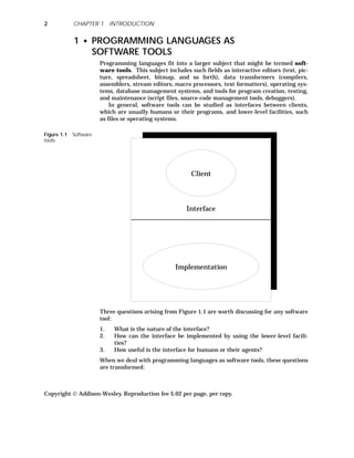
![Figure 1.11 for a := 1; Ptr := Start -- initialization 1
while Ptr ≠ nil -- termination condition 2
updating a := a+1; Ptr := Ptrˆ.Next; -- after each iter. 3
do 4
... -- loop body 5
end; 6
Russell and CSP generalize the nondeterministic if statement into a non-
deterministic while loop with multiple branches. So long as any guard is
true, the loop is executed, and any branch whose guard is true is arbitrarily
selected and executed. The loop terminates when all guards are false. For
example, the algorithm to compute the greatest common divisor of two inte-
gers a and b can be written as follows:
Figure 1.12 while 1
when a < b => b := b - a; 2
when b < a => a := a - b; 3
end; 4
Each guard starts with the reserved word when and ends with the symbol => .
The loop terminates when a = b.
The case statement is used to select one of a set of options on the basis of
the value of some expression.4
Most languages require that the selection be
based on a criterion known at compile time (that is, the case labels must be
constant or constant ranges); this restriction allows compilers to generate ef-
ficient code. However, conditions that can only be evaluated at runtime also
make sense, as in the following example:
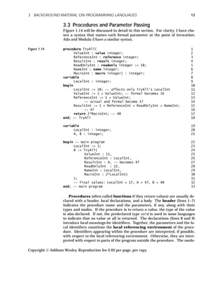
Figure 1.13 case a of 1
when 0 => Something(1); -- static unique guard 2
when 1..10 => Something(2); -- static guard 3
when b+12 => Something(3); -- dynamic unique guard 4
when b+13..b+20 => Something(4); -- dynamic guard 5
otherwise Something(5); -- guard of last resort 6
end; 7
Each guard tests the value of a. Lines 2 and 4 test this value for equality
with 0 and b+12; lines 3 and 5 test it for membership in a range. If the
guards (the selectors for the branches) overlap, the case statement is erro-
neous; this situation can be detected at compile time for static guards and at
runtime for dynamic guards. Most languages consider it to be a runtime er-
ror if none of the branches is selected and there is no otherwise clause.
hhhhhhhhhhhhhhhhhhhhhhhhhhhhhhhhhhhh
4
C. A. R. Hoare, who invented the case statement, says, “This was my first programming
language invention, of which I am still most proud.” [Hoare 73]
Copyright Addison-Wesley. Reproduction fee $.02 per page, per copy.
12 CHAPTER 1 INTRODUCTION](https://image.slidesharecdn.com/advancedprogramminglanguagedesign-230706034617-464d64c2/85/Advanced_programming_language_design-pdf-20-320.jpg)
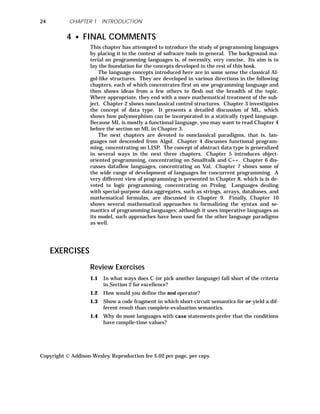
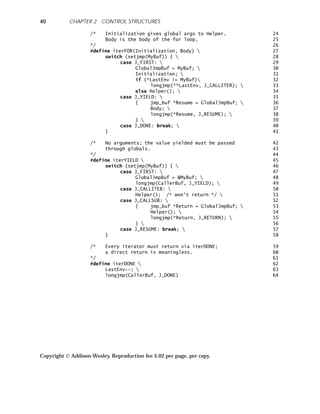
![25
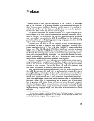
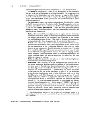
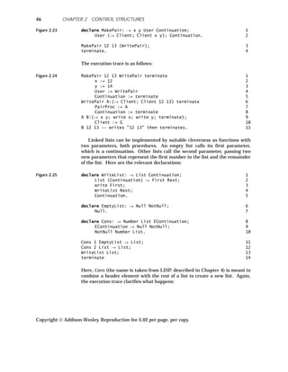
1.5 Write a procedure that produces different results depending on whether
its parameters are passed by value, reference, or name mode.
1.6 FORTRAN only passes parameters in reference mode. C only passes
parameters in value mode. Pascal allows both modes. Show how you
can get the effect of reference mode in C and how you can get the effect
of value mode in FORTRAN by appropriate programming techniques.
In particular, show in both FORTRAN and C how to get the effect of the
following code.
Figure 1.23 variable X, Y : integer; 1
procedure Accept 2
(A : reference integer; B: value integer); 3
begin 4
A := B; 5
B := B+1; 6
end; -- Accept 7
X := 1; 8
Y := 2; 9
Accept(X, Y); 10
-- at this point, X should be 2, and Y should be 2 11
1.7 If a language does not allow recursion (FORTRAN II, for example, did
not), is there any need for a central stack?
1.8 C does not allow a procedure to be declared inside another procedure,
but Pascal does allow nested procedure declarations. What effect does
this choice have on runtime storage organization?
Challenge Exercises
1.9 Why are array slices usually allowed only in the last dimension?
1.10 Write a program that prints the index of the first all-zero row of an n × n
integer matrix M [Rubin 88]. The program should access each element of
the matrix at most once and should not access rows beyond the first all-
zero row and columns within a row beyond the first non-zero element.
It should have no variables except the matrix M and two loop indices Row
and Column. The program may not use goto, but it may use multilevel
break and next.
1.11 What is the meaning of a goto from a procedure when the target is out-
side the procedure?
1.12 Why do goto labels passed as parameters require closures?
1.13 Rewrite Figure 1.21 (page 21) so that procedure A takes a label instead
of a procedure. The rewritten example should behave the same as Fig-
ure 1.21.
Copyright Addison-Wesley. Reproduction fee $.02 per page, per copy.
EXERCISES](https://image.slidesharecdn.com/advancedprogramminglanguagedesign-230706034617-464d64c2/85/Advanced_programming_language_design-pdf-33-320.jpg)
![h
hhhhhhhhhhhhhhhhhhhhhhhhhhhhhhhhhhhhhhhhhhhhhhhhhhhhhhhhhhhhhhhhhhhhhhhhhhhhhhhhhhhhhhhhhhh
Chapter 2 ❖
Control Structures
Assembler language only provides goto and its conditional variants. Early
high-level languages such as FORTRAN relied heavily on goto, three-way
arithmetic branches, and many-way indexed branches. Algol introduced con-
trol structures that began to make goto obsolete. Under the banner of “struc-
tured programming,” computer scientists such as C. A. R. Hoare, Edsger W.
Dijkstra, Donald E. Knuth, and Ole-Johan Dahl showed how programs could
be written more clearly and elegantly with while and for loops, case state-
ments, and loops with internal exits [Knuth 71; Dahl 72]. One of the tenets of
structured programming is that procedures should be used heavily to modu-
larize effort. In this chapter we will explore control structures that are a lit-
tle out of the ordinary.
1 ◆ EXCEPTION HANDLING
If a procedure discovers that an erroneous situation (such as bad input) has
arisen, it needs to report that fact to its caller. One way to program this be-
havior is to have each procedure provide an error return and to check for that
return on each invocation. SNOBOL allows an explicit failure goto and suc-
cess goto on each statement, which makes this sort of programming conve-
nient. However, using a goto to deal with errors does not lead to clear
programs, and checking each procedure invocation for error returns makes
for verbose programs.
A control construct for dealing with error conditions was first proposed by
Goodenough [Goodenough 75] and has found its way into languages like Ada,
Mesa, CLU, ML, Eiffel, and Modula-3. I will use a syntax like Ada’s for de-
scribing this control structure.
When a procedure needs to indicate failure, it raises an exception. This
action causes control to transfer along a well-defined path in the program to
where the exception is handled. To embed this concept in programming lan-
hhhhhhhhhhhhhhhhhhhhhhhhhhhhhhhhhhhh
On-line edition copyright 1996 by Addison-Wesley Publishing Company. Permission is
granted to print or photocopy this document for a fee of $0.02 per page, per copy, payable to Addi-
son-Wesley Publishing Company. All other rights reserved.
27](https://image.slidesharecdn.com/advancedprogramminglanguagedesign-230706034617-464d64c2/85/Advanced_programming_language_design-pdf-35-320.jpg)
![generate error messages that convey exactly which values were erroneous.
This problem is ameliorated in Modula-3, in which exceptions can take value-
mode parameters. The actual parameters are provided by the raise state-
ment, and the formal parameters are defined by the handle clause. Parame-
ters can be used to indicate where in the program the exception was raised
and what values led to the exceptional situation.
Second, programmer-defined exceptions may be visible in the raising
scope but not in the handling scope. The problem arises for programmer-
defined exceptions that exit the entire program (to a scope where only prede-
fined exceptions exist) and for “don’t-care” exception-handler patterns within
the program, as in line 4 below:
Figure 2.6 begin 1
... 2
handle 3
when _ => ... 4
end; 5
Such a handler might not be able to raise the exception further (unless the
programming language provides a predefined exception identifier Self that
holds the exception that was raised).
In some ways, raise statements are like goto statements to labels passed
as parameters. However, exceptions are far more disciplined than gotos, and
they do not require that the programmer pass targets as parameters.
Exceptions reduce the clarity of loop constructs. Every loop has an im-
plicit exit caused by an unhandled exception wresting control out of the loop.
Modula-3 unifies loops and exceptions by treating break as equivalent to
raise ExitException. Loop statements implicitly handle this exception and
exit the loop. Similarly, Modula-3 considers the return statement as equiva-
lent to raise ReturnException. The value returned by a function becomes
the parameter to ReturnException.
The exception mechanism I have shown binds exception handlers to
blocks. An alternative is to let raised exceptions throw the computation into
a failure state [Wong 90]. In failure state, ordinary statements are not exe-
cuted. Procedures can return while execution is in failure state, however.
Only the handle statement is executed in failure state; after it completes, fail-
ure state is no longer in force unless handle reraises an exception. The pro-
grammer may place handle statements in the middle of blocks, interspersed
with ordinary statements. The execution cost for this scheme may be fairly
high, however, because every statement must be compiled with a test to see if
execution is in failure state.
Exceptions are useful for more than handling error conditions. They also
provide a clean way for programs to exit multiple procedure invocations. For
example, an interactive editor might raise an exception in order to return to
the main command loop after performing a complex action.
Exceptions are not the only reasonable way to handle error conditions.
Sometimes it is easier for the programmer to have errors set a global variable
that the program may inspect later when it is convenient. For example, the
standard library packaged with C has a global variable errno that indicates
the most recent error that occurred in performing an operating-system call.
Copyright Addison-Wesley. Reproduction fee $.02 per page, per copy.
30 CHAPTER 2 CONTROL STRUCTURES](https://image.slidesharecdn.com/advancedprogramminglanguagedesign-230706034617-464d64c2/85/Advanced_programming_language_design-pdf-38-320.jpg)
![31
The programmer can choose to ignore return values and inspect errno well
into the calculation, redirecting further effort if an error has occurred. The
program is likely to be more efficient and clearer than a program that sur-
rounds code with exception handlers. This point is especially important in
numerical computations on large data sets on highly pipelined computers.
Putting in the necessary tests to handle exceptions can slow down such com-
putations so much that they become useless, whereas hardware that sets a
flag when it discovers overflow, say, allows such computations to run at full
speed and lets the program notice rare problems after the fact.
Another way to treat errors is by generating error values, such as unde-
fined and positive_overflow, that are an integral part of arithmetic types.
Similarly, null_pointer_dereference and array_range_error can be error
values generated by the related mistakes. Expressions can evaluate to an er-
ror value instead of their normal results. These error values are propagated
(using specific rules) to produce a final result. For example, 1/0 yields the
value zero_divide, while 0*(1/0) yields undefined. Any operation involving
zero_divide yields undefined. Error values render the results of all compu-
tations well defined, guaranteeing that all valid evaluation orders produce
the same result.1
They also provide for a degree of error repair, since the pro-
gram can test for error values and perhaps transform them into something
meaningful. However, because the program can continue computing with er-
ror values, the error values finally produced may provide no indication of the
original errors. It can be quite difficult to debug programs when errors prop-
agate in this way. It would be far more helpful if the error value contained
extra information, such as the source file and line number where the error oc-
curred, which could propagate along with the error value itself.
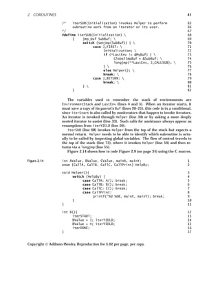
2 ◆ COROUTINES
Consider the problem of comparing two binary trees to see if their nodes have
the same values in symmetric (also called in-order) traversal. For example,
the trees in Figure 2.7 compare as equal.
Figure 2.7 Equivalent
binary trees
E
E
D
D
C
C
B
A B
A
We could use a recursive procedure to store the symmetric-order traversal in
an array, call the procedure for each tree, and then compare the arrays, but it
is more elegant to advance independently in each tree, comparing as we go.
Such an algorithm is also far more efficient if the trees are unequal near the
hhhhhhhhhhhhhhhhhhhhhhhhhhhhhhhhhhhh
1
An error algebra with good numeric properties is discussed in [Wetherell 83].
Copyright Addison-Wesley. Reproduction fee $.02 per page, per copy.
2 COROUTINES](https://image.slidesharecdn.com/advancedprogramminglanguagedesign-230706034617-464d64c2/85/Advanced_programming_language_design-pdf-39-320.jpg)
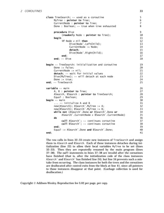
![2.2 Coroutines in CLU
The CLU language, designed by Barbara Liskov at MIT, provides a general-
ized for loop [Liskov 81]. The control variable takes on successive values
provided by a coroutine called an iterator. This iterator is similar in most
ways to an ordinary procedure, but it returns values via a yield statement.
When the for loop requires another value for the control variable, the itera-
tor is resumed from where it left off and is allowed to execute until it encoun-
ters another yield. If the iterator reaches the end of its code instead, the for
loop that relies on the iterator terminates. CLU’s yield is like Simula’s de-
tach, except that it also passes back a value. CLU’s for implicitly contains
the effect of Simula’s call.
A naive implementation of CLU would create a separate stack for each ac-
tive iterator instance. (The same iterator may have several active instances;
it does, for example, if there is a for nested within another for.) A coroutine
linkage, much like Simula’s call and detach, would ensure that each iterator
instance maintains its own context, so that it may be resumed properly.
The following program provides a simple example. CLU syntax is also
fairly close to Ada syntax; the following is almost valid CLU.
Figure 2.9 iterator B() : integer; -- yields 3, 4 1
begin 2
yield 3; 3
yield 4; 4
end; -- B 5
iterator C() : integer; -- yields 1, 2, 3 6
begin 7
yield 1; 8
yield 2; 9
yield 3; 10
end; -- C 11
iterator A() : integer; -- yields 10, 20, 30 12
variable 13
Answer : integer; 14
begin 15
for Answer := C() do -- ranges over 1, 2, 3 16
yield 10*Answer; 17
end; 18
end; -- A 19
variable 20
x, y : integer; 21
begin 22
for x := A() do -- ranges over 10, 20, 30 23
for y := B() do -- ranges over 3, 4 24
P(x, y); -- called 6 times 25
end; 26
end; 27
end; 28
The loop in line 23 iterates over the three values yielded by iterator A (lines
Copyright Addison-Wesley. Reproduction fee $.02 per page, per copy.
34 CHAPTER 2 CONTROL STRUCTURES](https://image.slidesharecdn.com/advancedprogramminglanguagedesign-230706034617-464d64c2/85/Advanced_programming_language_design-pdf-42-320.jpg)
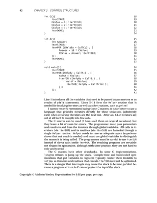
![35
12–19). For each of these values, the loop in line 24 iterates over the two val-
ues yielded by iterator B (lines 1–5). Iterator A itself introduces a loop that it-
erates over the three values yielded by iterator C (lines 6–11).
Happily, CLU can be implemented with a single stack. As a for loop be-
gins execution, some activation record (call it the parent) is active (although
not necessarily at the top of the stack). A new activation record for the itera-
tor is constructed and placed at the top of the stack. Whenever the body of
the loop is executing, the parent activation record is current, even though the
iterator’s activation record is higher on the stack. When the iterator is re-
sumed so that it can produce the next value for the control variable, its acti-
vation record again becomes current. Each new iterator invocation gets a
new activation record at the current stack top. Thus an activation record
fairly deep in the stack can be the parent of an activation record at the top of
the stack. Nonetheless, when an iterator terminates, indicating to its parent
for loop that there are no more values, the iterator’s activation record is cer-
tain to be at the top of the stack and may be reclaimed by simply adjusting
the top-of-stack pointer. (This claim is addressed in Exercise 2.10.)
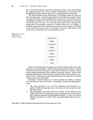
For Figure 2.9, each time P is invoked, the runtime stack appears as fol-
lows. The arrows show the dynamic (child-parent) chain.
Figure 2.10 Runtime
CLU stack during
iterator execution
iterator C
procedure P
iterator B
iterator A
main
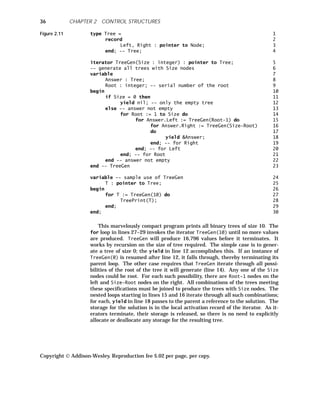
CLU iterators are often trivially equivalent to programs using ordinary
for loops. However, for some combinatorial algorithms, recursive CLU itera-
tors are much more powerful and allow truly elegant programs. One example
is the generation of all binary trees with n nodes. This problem can be solved
without CLU iterators, albeit with some complexity [Solomon 80]. Figure
2.11 presents a natural CLU implementation.
Copyright Addison-Wesley. Reproduction fee $.02 per page, per copy.
2 COROUTINES](https://image.slidesharecdn.com/advancedprogramminglanguagedesign-230706034617-464d64c2/85/Advanced_programming_language_design-pdf-43-320.jpg)
![39
3. Any routine that includes an iterFOR and every iterator must invoke
iterSTART at the end of local declarations.
4. Instead of falling through, iterators must terminate with iterDONE.
5. The Helper routine does not provide enough padding to allow iterators
and their callers to invoke arbitrary subroutines while iterators are on
the stack. Procedures must be invoked from inside iterFOR loops by
calling iterSUB.
The macro package appears in Figure 2.13. (Note for the reader unfamil-
iar with C: the braces { and } act as begin and end; void is a type with no
values; declarations first give the type (such as int or jmp_buf *) and then
the identifier; the assignment operator is = ; the dereferencing operator is * ;
the referencing operator is & .)
Figure 2.13 #include <setjmp.h> 1
#define ITERMAXDEPTH 50 2
jmp_buf *GlobalJmpBuf; /* global pointer for linkage */ 3
jmp_buf *EnvironmentStack[ITERMAXDEPTH] = {0}, 4
**LastEnv = EnvironmentStack; 5
/* return values for longjmp */ 6
#define J_FIRST 0 /* original return from setjmp */ 7
#define J_YIELD 1 8
#define J_RESUME 2 9
#define J_CALLITER 3 10
#define J_DONE 4 11
#define J_CALLSUB 5 12
#define J_RETURN 6 13
/* iterSTART must be invoked after all local declarations 14
in any procedure with an iterFOR and in all iterators. 15
*/ 16
#define iterSTART 17
jmp_buf MyBuf, CallerBuf; 18
if (GlobalJmpBuf) 19
bcopy((char *)GlobalJmpBuf, (char *)CallerBuf, 20
sizeof(jmp_buf)); 21
LastEnv++; 22
*LastEnv = &MyBuf; 23
Copyright Addison-Wesley. Reproduction fee $.02 per page, per copy.
2 COROUTINES](https://image.slidesharecdn.com/advancedprogramminglanguagedesign-230706034617-464d64c2/85/Advanced_programming_language_design-pdf-47-320.jpg)
![43
2.4 Coroutines in Icon
Icon is discussed in some detail in Chapter 9. It generalizes CLU iterators by
providing expressions that can be reevaluated to give different results.
3 ◆ CONTINUATIONS: IO
FORTRAN demonstrates that is possible to build a perfectly usable program-
ming language with only procedure calls and conditional goto as control
structures. The Io language reflects the hope that a usable programming lan-
guage can result from only a single control structure: a goto with parameters.
I will call the targets of these jumps procedures even though they do not re-
turn to the calling point. The parameters passed to procedures are not re-
stricted to simple values. They may also be continuations, which represent
the remainder of the computation to be performed after the called procedure
is finished with its other work. Instead of returning, procedures just invoke
their continuation. Continuations are explored formally in Chapter 10; here I
will show you a practical use.
Io manages to build remarkably sophisticated facilities on such a simple
foundation. It can form data structures by embedding them in procedures,
and it can represent coroutines.
Io programs do not contain a sequence of statements. A program is a pro-
cedure call that is given the rest of the program as a continuation parameter.
A statement continuation is a closure; it includes a procedure, its environ-
ment, and even its parameters.
Io’s syntax is designed to make statement continuations easy to write. If a
statement continuation is the last parameter, which is the usual case, it is
separated from the other parameters by a semicolon, to remind the program-
mer of sequencing. Continuations and procedures in other parameter posi-
tions must be surrounded by parentheses. I will present Io by showing
examples from [Levien 89].
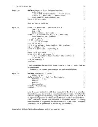
Figure 2.15 write 5; 1
write 6; 2
terminate 3
As you expect, this program prints 5 6. But I need to explain how it works.
The predeclared write procedure takes two parameters: a number and a con-
tinuation. The call in line 1 has 5 as its first parameter and write 6; termi-
nate as its second. The write procedure prints 5 and then invokes the
continuation. It is a call to another instance of write (line 2), with parame-
ters 6 and terminate. This instance prints 6 and then invokes the parame-
terless predeclared procedure terminate. This procedure does nothing. It
certainly doesn’t return, and it has no continuation to invoke.
Procedures can be declared as follows:
Figure 2.16 declare writeTwice: → Number; 1
write Number; write Number; terminate. 2
That is, the identifier writeTwice is associated with an anonymous procedure
Copyright Addison-Wesley. Reproduction fee $.02 per page, per copy.
3 CONTINUATIONS: IO](https://image.slidesharecdn.com/advancedprogramminglanguagedesign-230706034617-464d64c2/85/Advanced_programming_language_design-pdf-51-320.jpg)
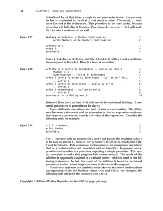
![49
4 ◆ POWER LOOPS
Although the programmer usually knows exactly how deeply loops must nest,
there are some problems for which the depth of nesting depends on the data.
Programmers usually turn to recursion to handle these cases; each level of
nesting is a new level of recursion. However, there is a clearer alternative
that can generate faster code. The alternative has recently2
been called
power loops [Mandl 90]. The idea is to have an array of control variables
and to build a loop that iterates over all control variables.
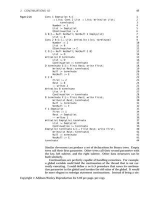
For example, the n-queens problem is to find all solutions to the puzzle of
placing n queens on an n × n chessboard so that no queen attacks any other.
Here is a straightforward solution:
Figure 2.28 variable 1
Queen : array 1 .. n of integer; 2
nest Column := 1 to n 3
for Queen[Column] := 1 to n do 4
if OkSoFar(Column) then 5
deeper; 6
end; -- if OkSoFar(Column) 7
end; -- for Queen[Column] 8
do 9
write(Queen[1..n]); 10
end; 11
Any solution will have exactly one queen in each column of the chessboard.
Line 2 establishes an array that will describe which row is occupied by the
queen in each column. The OkSoFar routine (line 5) checks to make sure that
the most recent queen does not attack (and therefore is not attacked by) any
of the previously placed queens. Line 3 introduces a set of nested loops. It ef-
fectively replicates lines 4–8 for each value of Column, placing the next replica
at the point marked by the deeper pseudostatement (line 6). There must be
exactly one deeper in a nest. Nested inside the innermost instance is the
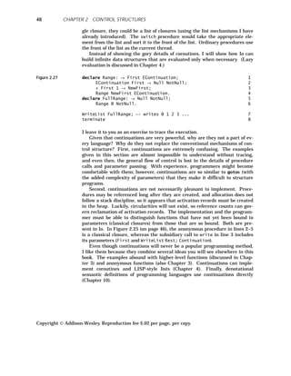
body shown in line 10. If n = 3, for example, this program is equivalent to the
code of Figure 2.29.
hhhhhhhhhhhhhhhhhhhhhhhhhhhhhhhhhhhh
2
The Madcap language had power loops in the early 1960s [Wells 63].
Copyright Addison-Wesley. Reproduction fee $.02 per page, per copy.
4 POWER LOOPS](https://image.slidesharecdn.com/advancedprogramminglanguagedesign-230706034617-464d64c2/85/Advanced_programming_language_design-pdf-57-320.jpg)
![Figure 2.29 for Queen[1] := 1 to n do 1
if OkSoFar(1) then 2
for Queen[2] := 1 to n do 3
if OkSoFar(2) then 4
for Queen[3] := 1 to n do 5
if OkSoFar(3) then 6
write(Queen[1..3]) 7
end; -- if 3 8
end; -- for 3 9
end; -- if 2 10
end; -- for 2 11
end; -- if 1 12
end; -- for 1 13
Nesting applies not only to loops, as Figure 2.30 shows.
Figure 2.30 nest Level := 1 to n 1
if SomeCondition(Level) then 2
deeper; 3
else 4
write("failed at level", Level); 5
end; 6
do 7
write("success!"); 8
end; 9
Of course, a programmer may place a nest inside another nest, either in the
replicated part (as in lines 2–6 of Figure 2.30) or in the body (line 8), but such
usage is likely to be confusing. If nest can be nested in the replicated part,
each deeper must indicate which nest it refers to.
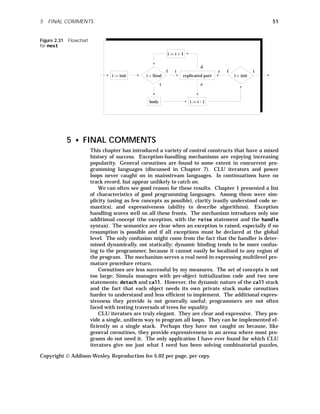
It is not hard to generate efficient code for nest. Figure 2.31 is a flowchart
showing the generated code, where i is the nest control variable. The labels t
and f are the true and false exits of the conditionals. Label d is the exit
from the replicated part when it encounters deeper, and r is the reentry after
deeper. The fall-through exit from the replicated part is called e. If execu-
tion after deeper will just fall through (as in Figure 2.30), decrementing i
and checking i < init can be omitted.
Although power loops are elegant, they are subsumed by recursive proce-
dures, albeit with a loss of elegance and efficiency. Power loops are so rarely
helpful that languages should probably avoid them. It doesn’t make sense to
introduce a construct in a general-purpose language if it will only be used in a
handful of programs.
Copyright Addison-Wesley. Reproduction fee $.02 per page, per copy.
50 CHAPTER 2 CONTROL STRUCTURES](https://image.slidesharecdn.com/advancedprogramminglanguagedesign-230706034617-464d64c2/85/Advanced_programming_language_design-pdf-58-320.jpg)

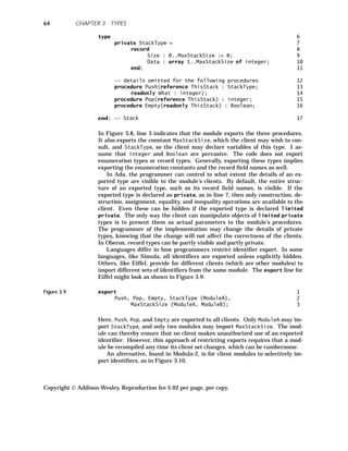
![57
3 ◆ TYPE EQUIVALENCE
The concept of strong typing relies on a definition of exactly when types are
equivalent. Surprisingly, the original definition of Pascal did not present a
definition of type equivalence. The issue can be framed by asking whether
the types T1 and T2 are equivalent in Figure 3.1:
Figure 3.1 type 1
T1, T2 = array[1..10] of real; 2
T3 = array[1..10] of real; 3
Structural equivalence states that two types are equivalent if, after all
type identifiers are replaced by their definitions, the same structure is ob-
tained. This definition is recursive, because the definitions of the type identi-
fiers may themselves contain type identifiers. It is also vague, because it
leaves open what “same structure” means. Everyone agrees that T1, T2, and
T3 are structurally equivalent. However, not everyone agrees that records re-
quire identical field names in order to have the same structure, or that arrays
require identical index ranges. In Figure 3.2, T4, T5, and T6 would be consid-
ered equivalent to T1 in some languages but not others:
Figure 3.2 type 1
T4 = array[2..11] of real; -- same length 2
T5 = array[2..10] of real; -- compatible index type 3
T6 = array[blue .. red] of real; -- incompatible 4
-- index type 5
Testing for structural equivalence is not always trivial, because recursive
types are possible. In Figure 3.3, types TA and TB are structurally equivalent,
as are TC and TD, although their expansions are infinite.
Figure 3.3 type 1
TA = pointer to TA; 2
TB = pointer to TB; 3
TC = 4
record 5
Data : integer; 6
Next : pointer to TC; 7
end; 8
TD = 9
record 10
Data : integer; 11
Next : pointer to TD; 12
end; 13
In contrast to structural equivalence, name equivalence states that two
variables are of the same type if they are declared with the same type name,
such as integer or some declared type. When a variable is declared using a
type constructor (that is, an expression that yields a type), its type is given
a new internal name for the sake of name equivalence. Type constructors in-
Copyright Addison-Wesley. Reproduction fee $.02 per page, per copy.
3 TYPE EQUIVALENCE](https://image.slidesharecdn.com/advancedprogramminglanguagedesign-230706034617-464d64c2/85/Advanced_programming_language_design-pdf-65-320.jpg)
![clude the words array, record, and pointer to. Therefore, type equivalence
says that T1 and T3 above are different, as are TA and TB. There are different
interpretations possible when several variables are declared using a single
type constructor, such as T1 and T2 above. Ada is quite strict; it calls T1 and
T2 different. The current standard for Pascal is more lenient; it calls T1 and
T2 identical [ANSI 83]. This form of name equivalence is also called declara-
tion equivalence.
Name equivalence seems to be the better design because the mere fact
that two data types share the same structure does not mean they represent
the same abstraction. T1 might represent the batting averages of ten mem-
bers of the Milwaukee Brewers, while T3 might represent the grade-point av-
erage of ten students in an advanced programming language course. Given
this interpretation, we surely wouldn’t want T1 and T3 to be considered equiv-
alent!
Nonetheless, there are good reasons to use structural equivalence, even
though unrelated types may accidentally turn out to be equivalent. Applica-
tions that write out their values and try to read them in later (perhaps under
the control of a different program) deserve the same sort of type-safety pos-
sessed by programs that only manipulate values internally. Modula-2+,
which uses name equivalence, outputs both the type name and the type’s
structure for each value to prevent later readers from accidentally using the
same name with a different meaning. Anonymous types are assigned an in-
ternal name. Subtle bugs arise if a programmer moves code about, causing
the compiler to generate a different internal name for an anonymous type.
Modula-3, on the other hand, uses structural equivalence. It outputs the
type’s structure (but not its name) with each value output. There is no dan-
ger that rearranging a program will lead to type incompatibilities with data
written by a previous version of the program.
A language may allow assignment even though the type of the expression
and the type of the destination variable are not equivalent; they only need to
be assignment-compatible. For example, under name equivalence, two ar-
ray types might have the same structure but be inequivalent because they
are generated by different instances of the array type constructor. Nonethe-
less, the language may allow assignment if the types are close enough, for ex-
ample, if they are structurally equivalent. In a similar vein, two types may
be compatible with respect to any operation, such as addition, even though
they are not type-equivalent. It is often a quibble whether to say a language
uses name equivalence but has lax rules for compatibility or to say that it
uses structural equivalence. I will avoid the use of “compatibility” and just
talk about equivalence.
Modula-3’s rules for determining when two types are structurally equiva-
lent are fairly complex. If every value of one type is a value of the second,
then the first type is a called a “subtype” of the second. For example, a record
type TypeA is a subtype of another record type TypeB only if their fields have
the same names and the same order, and all of the types of the fields of TypeA
are subtypes of their counterparts in TypeB. An array type TypeA is a subtype
of another array type TypeB if they have the same number of dimensions of
the same size (although the range of indices may differ) and the same index
and component types. There are also rules for the subtype relation between
procedure and pointer types. If two types are subtypes of each other, they are
Copyright Addison-Wesley. Reproduction fee $.02 per page, per copy.
58 CHAPTER 3 TYPES](https://image.slidesharecdn.com/advancedprogramminglanguagedesign-230706034617-464d64c2/85/Advanced_programming_language_design-pdf-66-320.jpg)
![tinct from integer. Similarly, 2 is a literal of type integer, not meters. Ada
solves this problem by overloading operators, procedures, and literals associ-
ated with a derived type. That is, when meters was created, a new set of
arithmetic operators and procedures (like sqrt) was created to take values of
type meters. Similarly, integer literals are allowed to serve also as meters
literals. The expression in line 8 is valid, but metric_length * impe-
rial_length involves a type mismatch.3
The compiler determines which version of an overloaded procedure, opera-
tor, and literal to use. Intuitively, it tries all possible combinations of inter-
pretations, and if exactly one satisfies all type rules, the expression is valid
and well defined. Naturally, a smart compiler won’t try all possible combina-
tions; the number could be exponential in the length of the expression. In-
stead, the compiler builds a collection of subtrees, each representing a
possible overload interpretation. When the root of the expression tree is
reached, either a unique overload resolution has been found, or the compiler
knows that no unique resolution is possible [Baker 82]. (If no appropriate
overloaded procedure can be found, it may still be possible to coerce the types
of the actual parameters to types that are accepted by a declared procedure.
However, type coercion is often surprising to the programmer and leads to
confusion.)
The concept of subtype can be generalized by allowing extensions and re-
ductions to existing types [Paaki 90]. For example, array types can be ex-
tended by increasing the index range and reduced by decreasing the index
range. Enumeration types can be extended by adding new enumeration con-
stants and reduced by removing enumeration constants. Record types can be
extended by adding new fields and reduced by removing fields. (Oberon al-
lows extension of record types.) Extending record types is very similar to the
concept of building subclasses in object-oriented programming, discussed in
Chapter 5.
The resulting types can be interconverted with the original types for pur-
poses of assignment and parameter passing. Conversion can be either by
casting or by coercion. In either case, conversion can ignore array elements
and record fields that are not needed in the target type and can set elements
and fields that are only known in the target type to an error value. It can
generate a runtime error if an enumeration value is unknown in the target
type.
The advantage of type extensions and reductions is much the same as that
of subclasses in object-oriented languages, discussed in Chapter 5: the new
type can make use of the software already developed for the existing type;
only new cases need to be specifically addressed in new software. A module
that extends or reduces an imported type does not force the module that ex-
ports the type to be recompiled.
hhhhhhhhhhhhhhhhhhhhhhhhhhhhhhhhhhhh
3
In Ada, a programmer can also overload operators, so one can declare a procedure that
takes a metric unit and an imperial unit, converts them, and then multiplies them.
Copyright Addison-Wesley. Reproduction fee $.02 per page, per copy.
60 CHAPTER 3 TYPES](https://image.slidesharecdn.com/advancedprogramminglanguagedesign-230706034617-464d64c2/85/Advanced_programming_language_design-pdf-68-320.jpg)
![61
4 ◆ DIMENSIONS
The example involving meters and feet shows that types alone do not pre-
vent programming errors. I want to prohibit multiplying two feet values and
assigning the result back into a feet variable, because the type of the result
is square feet, not feet.
The AL language, intended for programming mechanical manipulators, in-
troduced a typelike attribute of expressions called dimension to prevent
such errors [Finkel 76]. This concept was first suggested by C. A. R. Hoare
[Hoare 73], and it has been extended in various ways since then. Recent re-
search has shown how to include dimensions in a polymorphic setting like
ML [Kennedy 94]. (Polymorphism in ML is discussed extensively later in this
chapter.) AL has four predeclared base dimensions: time, distance, angle,
and mass. Each base dimension has predeclared constants, such as second,
centimeter, and gram. The values of these constants are with respect to an
arbitrary set of units; the programmer only needs to know that the constants
are mutually consistent. For example, 60*second = minute. New dimen-
sions can be declared and built from the old ones. AL does not support pro-
grammer-declared base dimensions, but such an extension would be
reasonable. Other useful base dimensions would be electrical current (mea-
sured, for instance, in amps), temperature (degrees Kelvin), luminous inten-
sity (lumens), and currency (florin). In retrospect, angle may be a poor choice
for a base dimension; it is equivalent to the ratio of two distances: distance
along an arc and the radius of a circle. Figure 3.7 shows how dimensions are
used.
Figure 3.7 dimension 1
area = distance * distance; 2
velocity = distance / time; 3
constant 4
mile = 5280 * foot; -- foot is predeclared 5
acre = mile * mile / 640; 6
variable 7
d1, d2 : distance real; 8
a1 : area real; 9
v1 : velocity real; 10
begin 11
d1 := 30 * foot; 12
a1 := d1 * (2 * mile) + (4 * acre); 13
v1 := a1 / (5 * foot * 4 * minute); 14
d2 := 40; -- invalid: dimension error 15
d2 := d1 + v1; -- invalid: dimension error 16
write(d1/foot, "d1 in feet", 17
v1*hour/mile, "v1 in miles per hour"); 18
end; 19
In line 13, a1 is the area comprising 4 acres plus a region 30 feet by 2 miles.
In line 14, the compiler can check that the expression on the right-hand side
has the dimension of velocity, that is, distance/time, even though it is hard
for a human to come up with a simple interpretation of the expression.
Copyright Addison-Wesley. Reproduction fee $.02 per page, per copy.
4 DIMENSIONS](https://image.slidesharecdn.com/advancedprogramminglanguagedesign-230706034617-464d64c2/85/Advanced_programming_language_design-pdf-69-320.jpg)
![63
type and to give clients only a limited view of these declarations. All declara-
tions that make up an abstract data type are placed in a module.4
It is a
name scope in which the programmer has control over what identifiers are
imported from and exported to the surrounding name scope. Local identifiers
that are to be seen outside a module are exported; all other local identifiers
are invisible outside the module, which allows programmers to hide imple-
mentation details from the clients of the module. Identifiers from surround-
ing modules are not automatically inherited by a module. Instead, those that
are needed must be explicitly imported. These features allow name scopes
to selectively import identifiers they require and provide better documenta-
tion of what nonlocal identifiers a module will need. Some identifiers, like
the predeclared types integer and Boolean, may be declared pervasive,
which means that they are automatically imported into all nested name
scopes.
Languages that support abstract data types often allow modules to be par-
titioned into the specification part and the implementation part. (Ada, Mod-
ula-2, C++, and Oberon have this facility; CLU and Eiffel do not.) The
specification part contains declarations intended to be visible to clients of
the module; it may include constants, types, variables, and procedure head-
ers. The implementation part contains the bodies (that is, implementa-
tions) of procedures as well as other declarations that are private to the
module. Typically, the specification part is in a separate source file that is re-
ferred to both by clients and by the implementation part, each of which is in a
separate source file.
Partitioning modules into specification and implementation parts helps
support libraries of precompiled procedures and separate compilation. Only
the specification part of a module is needed to compile procedures that use
the module. The implementation part of the module need not be supplied un-
til link time. However, separating the parts can make it difficult for imple-
mentation programmers to find relevant declarations, since they might be in
either part. One reasonable solution is to join the parts for the convenience of
the implementor and extract just the specification part for the benefit of the
compiler or client-application programmer.
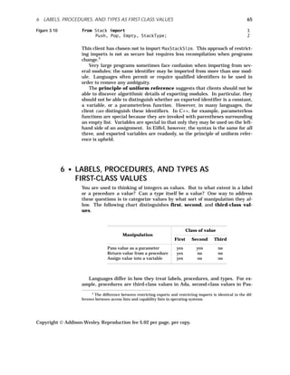
Figure 3.8 shows how a stack abstract data type might be programmed.
Figure 3.8 module Stack; 1
export 2
Push, Pop, Empty, StackType, MaxStackSize; 3
constant 4
MaxStackSize = 10; 5
hhhhhhhhhhhhhhhhhhhhhhhhhhhhhhhhhhhh
4
You can read a nice overview of language support for modules in [Calliss 91]. Modules are
used not only for abstract data types, but also for nesting name scopes, separate compilation, de-
vice control (in Modula, for example), and synchronization (monitors are discussed in Chapter 7).
Copyright Addison-Wesley. Reproduction fee $.02 per page, per copy.
5 ABSTRACT DATA TYPES](https://image.slidesharecdn.com/advancedprogramminglanguagedesign-230706034617-464d64c2/85/Advanced_programming_language_design-pdf-71-320.jpg)
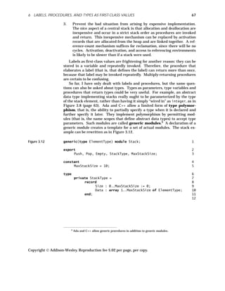
![-- details omitted for the following procedures 13
procedure Push(reference ThisStack : StackType; 14
readonly What : ElementType); 15
procedure Pop(reference ThisStack) : ElementType; 16
procedure Empty(readonly ThisStack) : Boolean; 17
end; -- Stack 18
module IntegerStack = Stack(integer); 19
To create an instance of a generic module, I instantiate it, as in line 19. In-
stantiation of generic modules in Ada and C++ is a compile-time, not a run-
time, operation — more like macro expansion than procedure invocation.
Compilers that support generic modules need to store the module text in or-
der to create instances.
The actual types that are substituted into the formal generic parameters
need not be built-in types like integer; program-defined types are also ac-
ceptable. However, the code of the generic module may require that the ac-
tual type satisfy certain requirements. For example, it might only make
sense to include pointer types, or array types, or numeric types. Ada provides
a way for generic modules to stipulate what sorts of types are acceptable. If
the constraint, for example, is that the actual type be numeric, then Ada will
permit operations like + inside the generic module; if there the constraint
only requires that assignment work, Ada will not allow the + operation.
Now, program-defined types may be numeric in spirit. For example, a com-
plex number can be represented by a record with two fields. Both Ada and
C++ allow operators like + to be overloaded to accept parameters of such
types, so that generic modules can accept these types as actual parameters
with a “numeric” flavor.
More general manipulation of types can also be desirable. Type construc-
tors like array or record can be viewed as predeclared, type-valued proce-
dures. It would be nice to be able to allow programmers to write such type
constructors. Although this is beyond the capabilities of today’s mainstream
languages, it is allowed in Russell, discussed later in this chapter. A much
fuller form of polymorphism is also seen in the ML language, the subject of
the next section.
7 ◆ ML
Now that I have covered some issues surrounding types, I will present a de-
tailed look at one of the most interesting strongly typed languages, ML
[Harper 89; Paulson 92]. ML, designed by Robin Milner, is a functional pro-
gramming language (the subject of Chapter 4), which means that procedure
calls do not have any side effects (changing values of variables) and that
there are no variables as such. Since the only reason to call a procedure is to
get its return value, all procedures are actually functions, and I will call them
that. Functions are first-class values: They can be passed as parameters, re-
turned as values from procedures, and embedded in data structures.
Higher-order functions (that is, functions returning other functions) are
used extensively. Function application is the most important control con-
Copyright Addison-Wesley. Reproduction fee $.02 per page, per copy.
68 CHAPTER 3 TYPES](https://image.slidesharecdn.com/advancedprogramminglanguagedesign-230706034617-464d64c2/85/Advanced_programming_language_design-pdf-76-320.jpg)
![ML programs can be grouped into separately compiled modules. Depen-
dencies among modules can be easily expressed, and the sharing of common
submodules is automatically guaranteed. ML keeps track of module versions
to detect compiled modules that are out of date.
I will describe some (by no means all!) of the features of SML, the Stan-
dard ML of New Jersey implementation [Appel 91]. I should warn you that I
have intentionally left out large parts of the language that do not pertain di-
rectly to the concept of type. For example, programming in the functional
style, which is natural to ML, is discussed in Chapter 4. If you find func-
tional programming confusing, you might want to read Chapter 4 before the
rest of this chapter. In addition, I do not discuss how ML implements ab-
stract data types, which is mostly similar to what I have covered earlier. I do
not dwell on one very significant type constructor: ref, which represents a
pointer to a value. Pointer types introduce variables into the language, be-
cause a program can associate an identifier with a pointer value, and the ob-
ject pointed to can be manipulated (assigned into and accessed). ML is
therefore not completely functional. The examples are syntactically correct
SML program fragments. I mark the user’s input by in and ML’s output by
out.
7.1 Expressions
ML is an expression-based language; all the standard programming con-
structs (conditionals, declarations, procedures, and so forth) are packaged as
expressions yielding values. Strictly speaking, there are no statements: even
operations that have side effects return values.
It is always meaningful to supply an arbitrary expression as the parame-
ter to a function (when the type constraints are satisfied) or to combine ex-
pressions to form larger expressions in the same way that simple constants
can be combined.
Arithmetic expressions have a fairly conventional appearance; the result
of evaluating an expression is presented by ML as a value and its type, sepa-
rated by a colon, as in Figure 3.13.
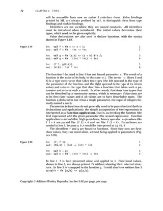
Figure 3.13 in: (3 + 5) * 2; 1
out: 16 : int 2
String expressions are straightforward (Figure 3.14).
Figure 3.14 in: "this is it"; 1
out: "this is it" : string 2
Tuples of values are enclosed in parentheses, and their elements are sepa-
rated by commas. The type of a tuple is described by the type constructor
* .7
hhhhhhhhhhhhhhhhhhhhhhhhhhhhhhhhhhhh
7
The * constructor, which usually denotes product, denotes here the set-theoretic Carte-
sian product of the values of the component types. A value in a Cartesian product is a compound
formed by selecting one value from each of its underlying component types. The number of val-
ues is the product of the number of values of the component types, which is one reason this set-
theoretic operation is called a product.
Copyright Addison-Wesley. Reproduction fee $.02 per page, per copy.
70 CHAPTER 3 TYPES](https://image.slidesharecdn.com/advancedprogramminglanguagedesign-230706034617-464d64c2/85/Advanced_programming_language_design-pdf-78-320.jpg)
![71
Figure 3.15 in: (3,4); 1
out: (3,4) : int * int 2
in: (3,4,5); 3
out: (3,4,5) : int * int * int 4
Lists are enclosed in square brackets, and their elements are separated by
commas, as in Figure 3.16. The list type constructor is the word list after
the component type.
Figure 3.16 in: [1,2,3,4]; 1
out: [1,2,3,4] : int list 2
in: [(3,4),(5,6)]; 3
out: [(3,4),(5,6)] : (int * int) list 4
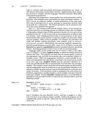
Conditional expressions have ordinary if syntax (as usual in expression-
based languages, else cannot be omitted), as in Figure 3.17.
Figure 3.17 in: if true then 3 else 4; 1
out: 3 : int 2
in: if (if 3 = 4 then false else true) 3
then false else true; 4
out: false : bool 5
The if part must be a Boolean expression. Two predeclared constants true
and false denote the Boolean values; the two binary Boolean operators
orelse and andalso have short-circuit semantics (described in Chapter 1).
7.2 Global Declarations
Values are bound to identifiers by declarations. Declarations can appear at
the top level, in which case their scope is global, or in blocks, in which case
they have a limited local scope spanning a single expression. I will first deal
with global declarations.
Declarations are not expressions. They establish bindings instead of re-
turning values. Value bindings are introduced by the keyword val; additional
value bindings are prefixed by and (Figure 3.18).
Figure 3.18 in: val a = 3 and 1
b = 5 and 2
c = 2; 3
out: val c = 2 : int 4
val b = 5 : int 5
val a = 3 : int 6
in: (a + b) div c; 7
out: 4 : int 8
In this case, I have declared the identifiers a, b, and c at the top level; they
Copyright Addison-Wesley. Reproduction fee $.02 per page, per copy.
7 ML](https://image.slidesharecdn.com/advancedprogramminglanguagedesign-230706034617-464d64c2/85/Advanced_programming_language_design-pdf-79-320.jpg)
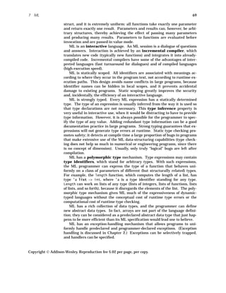
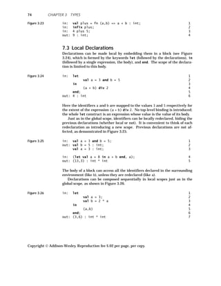
![73
Identifiers are statically scoped, and their values cannot change. When
new identifiers are declared, they may override previously declared identi-
fiers having the same name, but those other identifiers still exist and still re-
tain their old values. Consider Figure 3.21.
Figure 3.21 in: val a = 3; 1
out: val a = 3 : int 2
in: val f = fn x => a + x; 3
out: val f = fn : int -> int 4
in: val a = [1,2,3]; 5
out: val a = [1,2,3] : int list 6
in: f 1; 7
out: 4 : int 8
The function f declared in line 3 uses the top-level identifier a, which was
bound to 3 in line 1. Hence f is a function from integers to integers that re-
turns its parameter plus 3. Then a is redeclared at the top level (line 5) to be
a list of three integers; any subsequent reference to a will yield that list (un-
less it is redeclared again). But f is not affected at all: the old value of a was
frozen in f at the moment of its declaration, and f continues to add 3 to its ac-
tual parameter. The nonlocal referencing environment of f was bound when
it was first elaborated and is then fixed. In other words, ML uses deep bind-
ing.
Deep binding is consistent with static scoping of identifiers. It is quite
common in block-structured programming languages, but it is rarely used in
interactive languages like ML. The use of deep binding at the top level may
sometimes be counterintuitive. For example, if a function f calls a previously
declared function g, then redeclaring g (for example, to correct a bug) will not
change f, which will keep calling the old version of g.
The and keyword is used to introduce sets of independent declarations:
None of them uses the identifiers declared by the other bindings in the set;
however, a declaration often needs identifiers introduced by previous declara-
tions. The programmer may introduce such declarations sequentially, as in
Figure 3.22.
Figure 3.22 in: val a = 3; val b = 2 * a; 1
out: val a = 3 : int 2
val b = 6 : int 3
A function that expects a pair of elements can be converted to an infix op-
erator for convenience, as seen in line 2 of Figure 3.23.
Copyright Addison-Wesley. Reproduction fee $.02 per page, per copy.
7 ML](https://image.slidesharecdn.com/advancedprogramminglanguagedesign-230706034617-464d64c2/85/Advanced_programming_language_design-pdf-81-320.jpg)
![75
7.4 Lists
Lists are homogeneous; that is, all their components must have the same
type. The component type may be anything, such as strings, lists of integers,
and functions from integers to Booleans.
Many functions dealing with lists can work on lists of any kind (for exam-
ple to compute the length); they do not have to be rewritten every time a new
kind of list is introduced. In other words, these functions are naturally poly-
morphic; they accept a parameter with a range of acceptable types and return
a result whose type depends on the type of the parameter. Other functions
are more restricted in what type of lists they accept; summing a list makes
sense for integer lists, but not for Boolean lists. However, because ML allows
functions to be passed as parameters, programmers can generalize such re-
stricted functions. For example, summing an integer list is a special case of a
more general function that accumulates a single result by scanning a list and
applying a commutative, associative operation repeatedly to its elements. In
particular, it is not hard to code a polymorphic accumulate function that can
be used to sum the elements of a list this way, as in Figure 3.27.
Figure 3.27 in: accumulate([3,4,5], fn (x,y) => x+y, 0); 1
out: 12 : int 2
Line 1 asks for the list [3,4,5] to be accumulated under integer summation,
whose identity value is 0. Implementing the accumulate function is left as an
exercise.
The fundamental list constructors are nil, the empty list, and the right-
associative binary operator :: (pronounced “cons,” based on LISP, discussed
in Chapter 4), which places an element (its left operand) at the head of a list
(its right operand). The square-brackets constructor for lists (for example,
[1,2,3]) is an abbreviation for a sequence of cons operations terminated by
nil: 1 :: (2 :: (3 :: nil)). Nil itself may be written []. ML always uses
the square-brackets notation when printing lists.
Expression Evaluates to
nil []
1 :: [2,3] [1,2,3]
1 :: 2 :: 3 :: nil [1,2,3]
Other predeclared operators on lists include
• null, which returns true if its parameter is nil, and false on any other
list.
• hd, which returns the first element of a nonempty list.
• tl, which strips the first element from the head of a nonempty list.
• @ (append), which concatenates lists.
Hd and tl are called selectors, because they allow the programmer to select a
component of a structure. Here are some examples that use the predeclared
operators.
Copyright Addison-Wesley. Reproduction fee $.02 per page, per copy.
7 ML](https://image.slidesharecdn.com/advancedprogramminglanguagedesign-230706034617-464d64c2/85/Advanced_programming_language_design-pdf-83-320.jpg)
![Expression Evaluates to
null [] true
null [1,2,3] false
hd [1,2,3] 1
tl [1,2,3] [2,3]
[1,2] @ [] [1,2]
[] @ [3,4] [3,4]
[1,2] @ [3,4] [1,2,3,4]
Lists are discussed in greater depth in Chapter 4, which discusses functional
languages. They are interesting to us in this chapter because of their interac-
tion with ML’s type rules and with patterns.
7.5 Functions and Patterns
Because all functions take exactly one parameter, it is often necessary to pass
complicated structures in that parameter. The programmer may want the
formal parameter to show the structure and to name its components. ML
patterns provide this ability, as shown in Figure 3.28.
Figure 3.28 in: val plus = fn (a,b) => a + b;
I need to say a + b : int, as I will show later. Here, the function plus takes a
single parameter, which is expressed as a pattern showing that the parame-
ter must be a tuple with two elements, which are called formally a and b.8
This pattern does not force the actual parameter to be presented as an ex-
plicit tuple, as Figure 3.29 shows.
Figure 3.29 in: plus(3,4) 1
out: 7 : int 2
in: let 3
val x = (3,4) 4
in 5
plus x 6
end; 7
out: 7 : int 8
The first example (line 1) builds the actual parameter to plus explicitly from
two components, 3 and 4. The comma between them is the tuple constructor.
The syntax is contrived to remind the programmer that the intent is to pro-
vide two parameters.9
The second example presents a single variable x as the
actual parameter (line 6); the compiler can tell that it has the right type,
hhhhhhhhhhhhhhhhhhhhhhhhhhhhhhhhhhhh
8
The declaration is actually ambiguous; ML cannot determine which meaning of + is
meant.
9
In practice, a compiler can usually optimize away the extra pair constructions.
Copyright Addison-Wesley. Reproduction fee $.02 per page, per copy.
76 CHAPTER 3 TYPES](https://image.slidesharecdn.com/advancedprogramminglanguagedesign-230706034617-464d64c2/85/Advanced_programming_language_design-pdf-84-320.jpg)
![77
namely int * int.
Figure 3.30 shows how the declaration of plus can be written in single-
parameter form.
Figure 3.30 in: val plus = fn x => 1
let 2
val (a,b) = x 3
in 4
a + b 5
end; 6
out: val plus = fn : int * int -> int
This example avoids a pattern for the formal parameter, now called x (line 1).
However, it introduces a pattern in line 3 to produce the same effect. This
pattern constrains x (retroactively) to be a pair, and it binds a and b to the
two components. Figure 3.31 also uses patterns, both in specifying formal pa-
rameters and in declaring identifiers.
Figure 3.31 in: val f = fn [x,y,z] => (x,y,z); 1
out: val f = fn : ’a list -> ’a * ’a * ’a 2
in: val (a,b,c) = f[1,2,3]; 3
out: val c = 3 : int 4
val b = 2 : int 5
val a = 1 : int 6
The function f (line 1) returns three values packaged as a tuple. The pattern
a,b,c in line 3 is used to unpack the result of f[1,2,3] into its components.
Patterns in ML come in many forms. For example, a pattern [a,b,c]
matches a list of exactly three elements, which are mapped to a, b, and c; a
pattern first::rest matches a nonempty list with its first element associ-
ated with first, and its other elements to rest. Similarly,
first::second::rest matches a list with at least two elements, and so forth.
The most common patterns are tuples like (a,b,c), but more complicated
patterns can be constructed by nesting, such as ([a,b],c,(d,e)::h). The
don’t-care pattern h matches any value without establishing any binding.
Patterns can conveniently replace selector operators for unpacking data.
Patterns allow functions to be coded using case analysis, that is, testing
the value of the parameter to determine which code to execute. This situa-
tion is most common in recursive functions, which must first test if the pa-
rameter is the base case, which is treated differently from other cases. ML
programs seldom need to use the if expression for this purpose. Instead, pat-
tern alternatives are used, as in Figure 3.32.
Figure 3.32 in: val rec summation = 1
fn nil => 0 2
| (head :: tail) => head + summation tail; 3
out: val summation = fn : int list -> int 4
The rec declaration in line 1 indicates that the scope of the declaration of
Copyright Addison-Wesley. Reproduction fee $.02 per page, per copy.
7 ML](https://image.slidesharecdn.com/advancedprogramminglanguagedesign-230706034617-464d64c2/85/Advanced_programming_language_design-pdf-85-320.jpg)
![summation starts immediately, not after the declaration. This wide scope al-
lows the invocation of summation in line 3 to refer to this function itself. The
formal parameter is presented as a series of alternatives separated by the
| symbol. Each alternative gives a different pattern, thereby restricting the
allowable values of the actual parameter and naming its formal components.
The patterns are evaluated sequentially when the function is invoked. If a
pattern matches the actual parameter, the identifiers in the pattern act as
formal parameters that are bound to the respective parts of the actual param-
eter, and the corresponding action is executed. If several patterns match the
actual parameter, only the first matching one is activated. If all patterns fail
to match the actual parameter, a runtime exception occurs. In this case, the
first pattern requires that the parameter be an empty list; the second
matches any nonempty list and names its components head and tail.10
Patterns used for case analysis should obey several properties. First, they
must all be of the same type. In Figure 3.32, both nil and (head :: tail) are
of a list type with unspecified component type. ML disallows a declaration in
which the formal-parameter patterns cannot be unified into a single type.
Second, they should be exhaustive, covering all possible cases. The ML com-
piler will issue a warning if it detects a nonexhaustive match. (In the exam-
ple, omitting either of the two cases elicits such a warning.) Invoking a
function with a nonexhaustive match can lead to a Match exception being
raised (exceptions are discussed in Chapter 2). Third, good style dictates that
they should not overlap. The ML compiler issues a warning if it detects a re-
dundant match. The first matching pattern will be used when the function is
invoked.
Patterns are found in other languages as well. CSP (Chapter 7) and Pro-
log (Chapter 8) use patterns both for unpacking parameters and for introduc-
ing restrictions on their values. String-processing languages (Chapter 9) use
patterns for testing data and extracting components.
7.6 Polymorphic Types
A function is polymorphic when it can work uniformly over parameters of
different data types. For example, the function in Figure 3.33 computes the
length of a list.
Figure 3.33 in: val rec length = 1
fn nil => 0 2
| (h :: tail) => 1 + length tail; 3
out: val length = fn : ’a list -> int 4
in: (length [1,2,3], length ["a","b","c","d"]); 5
out: (3,4) : int * int 6
The type of length inferred by the compiler (line 4) contains a type identifier
(’a), indicating that any kind of list can be used, such as an integer list or a
hhhhhhhhhhhhhhhhhhhhhhhhhhhhhhhhhhhh
10
The parentheses in the second pattern are not needed; I put them in for the sake of clari-
ty. Parentheses are required in tuples, however.
Copyright Addison-Wesley. Reproduction fee $.02 per page, per copy.
78 CHAPTER 3 TYPES](https://image.slidesharecdn.com/advancedprogramminglanguagedesign-230706034617-464d64c2/85/Advanced_programming_language_design-pdf-86-320.jpg)
![79
string list. A type identifier is any ordinary identifier prefixed by one or more
tic marks (’). For convenience, we can pronounce ’a as “alpha” and ’b as
“beta.”
A type is polymorphic if it contains type identifiers; otherwise it is
monomorphic. A type identifier can be mapped to any ML type and thereby
form an instance of that type. For example, int list is a monomorphic in-
stance of ’a list. Instances of polymorphic types may themselves be poly-
morphic. For example, (’b * ’c) list is a polymorphic instance of ’a list.
Several type identifiers can be used in a type, and each identifier can ap-
pear several times, expressing contextual relationships between components
of a type. For example, ’a * ’a is the type of all pairs having components of
the same type. Contextual constraints can also be expressed between param-
eters and results of functions, as in the identity function, which has type ’a
-> ’a, or the function in Figure 3.34, which swaps pairs:
Figure 3.34 in: val swap = fn (x,y) => (y,x); 1
out: val swap = fn : (’a * ’b) -> (’b * ’a) 2
in: swap ([],"abc"); 3
out: ("abc",[]) : string * (’a list) 4
The empty list [] is a polymorphic expression of type ’a list, because it can
be considered an empty integer list, an empty string list, or some other empty
list.
In printing out polymorphic types, ML uses the type identifiers ’a, ’b, and
so on in succession, starting again from ’a at every new top-level declaration.
Several primitive functions are polymorphic. For example, you have al-
ready encountered the list operators, whose types appear in the following
table.
Operator Type
nil ’a list
:: (’a * ’a list) -> ’a list
null (’a list) -> bool
hd (’a list) -> ’a
tl (’a list) -> (’a list)
@ (’a list * ’a list) -> (’a list)
If these operators were not polymorphic, a program would need different
primitive operators for all possible types of list elements. The ’a shared by
the two parameters of :: (cons) prevents any attempt to build lists containing
expressions of different types.
The user can always determine the type of any ML function or expression
by typing its name at the top level; the expression is evaluated and, as usual,
its type is printed after its value, as in Figure 3.35.
Copyright Addison-Wesley. Reproduction fee $.02 per page, per copy.
7 ML](https://image.slidesharecdn.com/advancedprogramminglanguagedesign-230706034617-464d64c2/85/Advanced_programming_language_design-pdf-87-320.jpg)
![Figure 3.35 in: []; 1
out: [] : ’a list 2
in: hd; 3
out: fn : (’a list) -> ’a 4
7.7 Type Inference
A type can be a type identifier (’a, ’b, ...), or it can be constructed with type
constructors. Predeclared type constants, like int and bool, are actually
nullary type constructors. Polymorphic type constructors include -> , * ,
and list.
As a simple example of type inference, if I declare Identity = fn x =>
x, then Identity has type ’a -> ’a, because it returns unchanged expressions
of any type. If I have the application Identity 0, then since 0 is of type int,
this application of Identity is specialized to int -> int, and hence the value
of the application is of type int.
The following table summarizes the types assumed for a variety of literals
and operators, some of which are naturally polymorphic.
Expression Type
true bool
false bool
1 int
+ (int * int) -> int
= (’a * ’a) -> bool
nil ’a list
:: (’a * ’a list) -> ’a list
hd ’a list -> ’a
tl ’a list -> ’a list
null ’a list -> bool
A type expression may contain several occurrences of the same type iden-
tifier, allowing the programmer to specify type dependencies. Thus ’a -> ’a
represents a function whose parameter and result type are the same, al-
though it does not specify what that type is. In a type expression, all occur-
rences of a type identifier must represent the same type. Discovering that
type is done by an algorithm called unification; it finds the strongest com-
mon type constraint for (possibly polymorphic) types. For example, int ->
int and (int -> bool) -> (int -> bool) can be unified to ’a -> ’a. They can
also be unified to ’a -> ’b, but that is a weaker constraint. In fact, they can
be unified to the weakest possible type, ’a.
To perform polymorphic type inference, ML assigns a type identifier to
each expression whose type is unknown and then solves for the type identi-
fiers. The algorithm to solve for the type identifiers is based on repeatedly
applying constraints:
Copyright Addison-Wesley. Reproduction fee $.02 per page, per copy.
80 CHAPTER 3 TYPES](https://image.slidesharecdn.com/advancedprogramminglanguagedesign-230706034617-464d64c2/85/Advanced_programming_language_design-pdf-88-320.jpg)
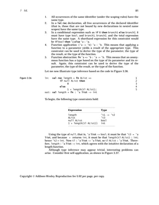
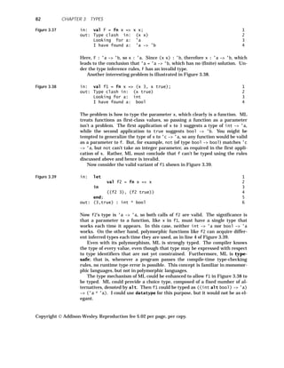
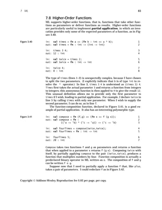
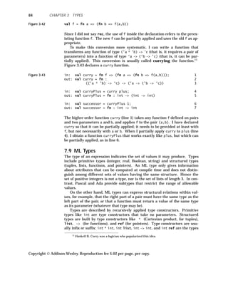
![85
of integer pairs, lists, functions, and pointers. Type constructors can be arbi-
trarily nested. For example, (int -> int) list is the type of lists of integer-
to-integer functions.
Type identifiers can be used to express polymorphic types. Polymorphic
types are mostly useful as types of functions, although some nonfunctional
expressions, like [], of type ’a list, are also polymorphic. A typical example
of a polymorphic function is hd, of type ’a list -> ’a. The type of hd indi-
cates that it can accept any list and that the type of the result is the same as
the type of the elements of the list.
Every type denotes a type domain, which is the set of all values of the
given type. For example, int * int denotes the domain of integer pairs, and
int -> int denotes the domain of all integer functions. An expression can
have several types; that is, it can belong to several domains. For example,
the identity function fn x => x has type int -> int, because it maps any ex-
pression of type integer to itself, but it also has the type bool -> bool for a
similar reason. The most general polymorphic type for the identity function
is ’a -> ’a, because all the types of identity are instances of it. This last nota-
tion gives more information than the others, because it encompasses all the
types that the identity function can have and thus expresses all the ways that
the identity function can be used. Hence it is preferable to the others, al-
though the others are not wrong. The ML type checker always determines
the most general type for an expression, given the information contained in
that expression.
The programmer may append a type expression to a data expression in or-
der to indicate a type constraint, as in Figure 3.44.
Figure 3.44 in: 3 : int; 1
out: 3 : int 2
in: [(3,4), (5,6) : int * int]; 3
out: [(3,4),(5,6)] : (int * int) list 4
In this example, the type constraint has no effect. The compiler indepen-
dently infers the types and checks them against the given constraints. Any
attempt to constrain a type incorrectly will result in a type error, as shown in
Figure 3.45.
Figure 3.45 in: 3 : bool; 1
out: Type clash in: 3 : bool 2
Looking for a: bool 3
I have found a: int 4
However, a type constraint can restrict the types inferred by ML by con-
straining polymorphic expressions or functions, as in Figure 3.46.
Copyright Addison-Wesley. Reproduction fee $.02 per page, per copy.
7 ML](https://image.slidesharecdn.com/advancedprogramminglanguagedesign-230706034617-464d64c2/85/Advanced_programming_language_design-pdf-93-320.jpg)
![Figure 3.46 in: [] : int list; 1
out: [] : int list 2
in: (fn x => x) : int -> int; 3
out: fn : int -> int 4
The type normally inferred for [] is ’a list, and for fn x => x, it is ’a -> ’a.
Type constraints can be used in declarations, as in Figure 3.47.
Figure 3.47 in: val (a : int) = 3; 1
in: val f = fn (a : int, b : int) => a+b; 2
in: val f = fn (a : int, b) => a+b; 3
in: val f = fn ((a,b) : int * int) => (a + b) : int; 4
The examples in lines 2, 3, and 4 are equivalent.
7.10 Constructed Types
A constructed type is a type for which constructors are available. Con-
structors can be used in patterns later to decompose data. You have already
seen examples of this dual usage with the tuple constructor and the list con-
structors nil and :: (cons).
A constructed type and its constructors should be considered as a single
conceptual unit. Whenever a new constructed type is declared, its construc-
tors are declared at the same time. Wherever a constructed type is known,
its constructors are also known.
The programmer can introduce new constructed types in a type declara-
tion. A type declaration introduces a new type name and the names of the
constructors for that type. Each of those constructors leads to a component,
whose type is also presented. The components together make up a choice
type, that is, a type whose values cover all the components. Syntactically,
components are separated by | . Each component starts with its constructor
name, followed by the keyword of and then the type of the component. The
keyword of and the component type can be omitted; in this case the construc-
tor is a constant of the new type.
For example, money can be a coin of some value (in cents), a bill of some
value (in dollars), a check drawn on some bank for some amount (in cents), or
the absence of money (see Figure 3.48).
Figure 3.48 in: datatype money = 1
nomoney | 2
coin of int | 3
bill of int | 4
check of string * int; -- (bank, cents) 5
Copyright Addison-Wesley. Reproduction fee $.02 per page, per copy.
86 CHAPTER 3 TYPES](https://image.slidesharecdn.com/advancedprogramminglanguagedesign-230706034617-464d64c2/85/Advanced_programming_language_design-pdf-94-320.jpg)
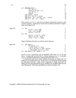
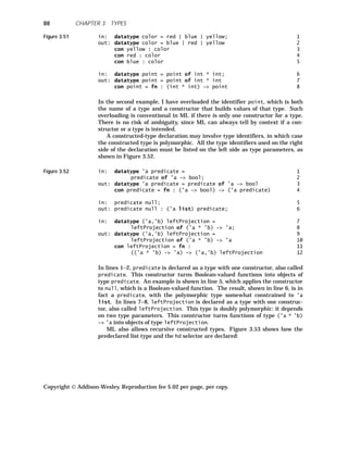
![89
Figure 3.53 in: datatype ’a list = 1
nil | 2
:: of ’a * (’a list); 3
out: datatype ’a list = 4
nil | 5
:: of ’a * (’a list) 6
con nil : ’a list 7
con :: = fn : (’a * (’a list)) -> (’a list) 8
in: val hd = fn ::(head, rest) => head; 9
out: val hd = fn : (’a list) -> ’a 10
The pattern in line 9 indicates that hd may only be called on lists constructed
with the :: constructor; it is invalid to call it on nil.
In addition to constructed types, ML provides abstract data types through
a module mechanism. It permits the specification and the implementation
parts to be separated. Modules can be parameterized by types, in much the
same way as generic modules in Ada and C++.
Before leaving the subject of types, I will turn briefly to two other pro-
gramming languages that are closely related to ML but show how one might
extend its treatment of types.
8 ◆ MIRANDA
The Miranda language, designed by David Turner of the University of Kent,
shares many features with ML [Turner 85a, 86; Thompson 86]. It is strongly
typed, infers types from context, provides for abstract data types, and has
higher-order functions. It provides tuples and homogeneous lists, and compo-
nents of tuples are extracted by patterns. Operators are provided for cons
and append, as well as for list length, selection from a list by position, and set
difference.
Miranda differs from ML in some minor ways. It is purely functional;
there are no pointer types. Functions of more than one parameter are auto-
matically curried unless parentheses explicitly indicate a tuple. (ML also has
a declaration form that automatically curries, but I have not shown it.) The
scope rules in Miranda are dynamic, which means that functions may be ref-
erenced textually before they are declared. All declarations implicitly allow
recursion; there is no need for a rec keyword. Binary operators may be
passed as actual parameters in Miranda; they are equivalent to curried func-
tions that take two parameters.
Miranda has a nontraditional syntax in which indentation indicates
grouping and conditionals look like the one in Figure 3.54.
Figure 3.54 max = a, a>=b 1
= b, otherwise 2
However, my examples will follow ML syntax (modified as necessary) for con-
sistency.
Miranda provides some novel extensions to ML. First, evaluation is nor-
mally lazy. I discuss lazy evaluation in detail in Chapter 4; for now, let me
Copyright Addison-Wesley. Reproduction fee $.02 per page, per copy.
8 MIRANDA](https://image.slidesharecdn.com/advancedprogramminglanguagedesign-230706034617-464d64c2/85/Advanced_programming_language_design-pdf-97-320.jpg)
![just say that expressions, particularly actual parameters, are not evaluated
until they must be, and then only as much as necessary. As Figure 3.55
shows, I can declare a function cond that does not need to evaluate all its pa-
rameters.
Figure 3.55 in: val cond = 1
fn true, x, y => x 2
| false, x, y => y; 3
out: val cond = fn : bool -> (’a -> (’a -> ’a)) 4
in: let val x=0 in cond x=0 0 1/x end 5
out: 0 : int 6
If cond evaluated all its parameters, the invocation in line 5 would generate
an exception as the program tries to divide 1 by 0. However, lazy evaluation
prevents the suspicious parameter from being evaluated until it is needed,
and it is never needed.
Miranda provides a concise syntax for specifying lists by enumerating
their components. Most simply, one can build a list by a shorthand, as in Fig-
ure 3.56.
Figure 3.56 in: [1..10]; 1
out: [1, 2, 3, 4, 5, 6, 7, 8, 9, 10] : int list 2
Infinite lists (Figure 3.57) are a bit more sophisticated.
Figure 3.57 in: [0..]; 1
out: [0, 1, 2, ...] : int list 2
in: val ones = 1 :: ones; 3
out: [1, 1, 1, ...] : int list 4
Line 3 declares ones recursively. I have arbitrarily decided to let the expres-
sion printer evaluate only the first three components of an infinite list.
The next step is to filter objects, whether finite or infinite, to restrict val-
ues. ZF-expressions (named after Zermelo and Fraenkel, founders of modern
set theory), also called list comprehensions, are built out of filters, as shown
in Figure 3.58.
Copyright Addison-Wesley. Reproduction fee $.02 per page, per copy.
90 CHAPTER 3 TYPES](https://image.slidesharecdn.com/advancedprogramminglanguagedesign-230706034617-464d64c2/85/Advanced_programming_language_design-pdf-98-320.jpg)
![91
Figure 3.58 in: [n*n | n <- [1..5] ]; 1
out: [1, 4, 9, 16, 25] : int list 2
in: [ (a,b,c,n) | a,b,c,n <- [3..]; aˆn + bˆn = cˆn ]; 3
out: [ ... ] : (int * int * int * int) list 4
in: val QuickSort = 5
fn [] => [] 6
| (a :: rest) => 7
QuickSort [ b | b <- rest; b <= a ] @ 8
[a] @ 9
QuickSort [ b | b <- rest; b > a]; 10
out: val QuickSort = fn : ’a list -> ’a list 11
Line 1 evaluates to a list of 5 squares. Line 3 evaluates to an empty list (most
likely), but will take forever to compute. However, if the expression is evalu-
ated lazily, the infinite computation need not even start. Lines 5–10 repre-
sent the Quicksort algorithm concisely.
Infinite lists can be used to create lookup tables for caching the values of a
function. Caching allows a programmer to use a recursive algorithm but ap-
ply caching (also called dynamic programming and memoization) to change
an exponential-time algorithm into a linear-time one. For example, Fibonacci
numbers can be computed efficiently as shown in Figure 3.59.
Figure 3.59 in: val map = 1
fn function, [] => [] 2
| function, [a :: rest] => 3
(function a) :: (map function rest); 4
out: val map = fn : (’a -> ’b) -> (’a list -> ’b list) 5
in: val cache = map fib [0..] 6
and fib = 7
fn 0 = 1 8
| 1 => 1 9
| n => cache at (n-1) + cache at (n-2) 10
out: val fib = fn : int -> int 11
The map function (lines 1–4) applies a function to each member of a list, pro-
ducing a new list. The fib function (lines 7–10) uses the infinite object cache
(line 6), which is not evaluated until necessary. Line 10 calls for evaluating
just those elements of cache that are needed. (The at operator selects an ele-
ment from a list on the basis of its position.) The chart in Figure 3.60 shows
the order of events in evaluating fib 4.
Copyright Addison-Wesley. Reproduction fee $.02 per page, per copy.
8 MIRANDA](https://image.slidesharecdn.com/advancedprogramminglanguagedesign-230706034617-464d64c2/85/Advanced_programming_language_design-pdf-99-320.jpg)
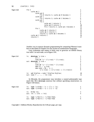
![93
in: type BoolMatrix = Matrix bool; 7
out: type BoolMatrix = bool list list 8
in: val AMatrix = [[true, false] [false, false]] 9
: BoolMatrix; 10
out: val AMatrix = [[true, false] [false, false]] 11
: bool list list 12
in: val FirstRow = fn 13
[RowOne :: OtherRows] : BoolMatrix => RowOne; 14
out: val FirstRow = fn : 15
bool list list -> bool list 16
In line 1, BinOp is declared as a polymorphic type with one type parameter,
’a. Line 3 demonstrates that BinOp can be invoked with a parameter int,
leading to the type int -> (int -> int). Types derived from polymorphic
types may be used to constrain declarations, as seen trivially in lines 9–10
and not so trivially in lines 13–14.
Recursively defined types sometimes need to provide multiple ways of de-
riving the same object. For example, if I wish to declare integers as a recur-
sive data type with constructors succ and pred, I need to indicate that zero is
the same as succ(pred zero). Miranda allows the programmer to specify
simplification laws, as shown in Figure 3.63.
Figure 3.63 in: datatype MyInt = 1
zero | 2
pred of MyInt | 3
succ of MyInt 4
laws 5
pred(succ n) => n and succ(pred n) => n; 6
in: pred(pred(succ(zero)); 7
out: pred zero : MyInt 8
Simplification laws also allow the programmer to declare a rational-number
data type that stores numbers in their canonical form (see Figure 3.64).
Figure 3.64 in: datatype Rational = ratio of num * num 1
laws ratio (a,b) => 2
if b = 0 then 3
error "zero denominator" 4
elsif b < 0 then 5
ratio (-a,-b) 6
Copyright Addison-Wesley. Reproduction fee $.02 per page, per copy.
8 MIRANDA](https://image.slidesharecdn.com/advancedprogramminglanguagedesign-230706034617-464d64c2/85/Advanced_programming_language_design-pdf-101-320.jpg)
![else 7
let 8
val gcd = fn (x,y) => 9
if a < b then gcd (a,b-a) 10
elsif b < a then gcd (a-b,b) 11
else a; 12
CommonPart = gcd (abs a, abs b) 13
in 14
if CommonPart > 1 then 15
ratio (a div CommonPart, 16
b div CommonPart); 17
else 18
nosimplify 19
end; 20
in: ratio (3,2); 21
out: ratio (3,2) : Rational 22
in: ratio (12,-3); 23
out: ratio (-4,1) : Rational 24
In line 19, nosimplify indicates that no law applies in that case.
9 ◆ RUSSELL
The Russell language predates ML but is quite similar in general flavor
[Demers 79; Boehm 86]. It was developed to explore the semantics of types,
in particular, to try to make types first-class values. Russell is strongly
typed, infers types from context, provides for abstract data types, and has
higher-order functions.
Russell differs from ML in some minor ways. Although it is statically
scoped, new function declarations do not override old ones of the same name
if the types differ; instead, the name becomes overloaded, and the number
and type of the actual parameters are used to distinguish which function is
meant in any particular context. (Redeclaration of identifiers other than
functions is not allowed at all.) Functions may be declared to be invoked as
prefix, suffix, or infix operators. Functions that take more than two parame-
ters may still be declared to be invoked with an infix operator; a given num-
ber of the parameters are placed before the operator, and the rest after. ML
only allows infix notation for binary functions. To prevent side effects in the
presence of variables (ref types), functions do not import identifiers mapped
to variables.
Russell’s nomenclature is nonstandard; what ML calls a type is a signa-
ture in Russell; an abstract data type (a collection of functions) is a type in
Russell. So when Russell succeeds in making types first-class values, it
doesn’t accomplish quite as much as we would expect. Russell’s syntax is
quite different from ML. For consistency, I will continue to use ML terminol-
ogy and syntax as I discuss Russell.
The principal difference between Russell and ML is that in Russell ab-
stract data types are first-class values, just like values, pointers, and func-
tions. That is, abstract data types may be passed as parameters, returned
from functions, and stored in identifiers. Abstract data type values can also
be manipulated after they have been constructed.
More specifically, Russell considers an abstract data type to be a collection
of functions that may be applied to objects of a particular domain. The
Boolean abstract data type includes the nullary functions true and false, bi-
nary operators such as and and or, and even statements such as if and
while, which have Boolean components. Manipulation of an abstract data
type means deleting or inserting functions in its definition.
The border between data and program becomes quite blurred if we look at
the world this way. After all, we are not used to treating control constructs
like while as functions that take two parameters, a Boolean and a statement,](https://image.slidesharecdn.com/advancedprogramminglanguagedesign-230706034617-464d64c2/85/Advanced_programming_language_design-pdf-102-320.jpg)
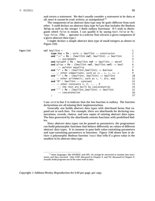
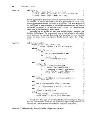
![97
10 ◆ DYNAMIC TYPING IN STATICALLY TYPED
LANGUAGES
It seems strange to include dynamic typing in otherwise statically typed lan-
guages, but there are situations in which the types of objects cannot be pre-
dicted at compile time. In fact, there are situations in which a program may
wish to create a new type during its computation.
An elegant proposal for escaping from static types is to introduce a prede-
clared type named dynamic [Abadi 91]. This method is used extensively in
Amber [Cardelli 86]. Values of this type are constructed by the polymorphic
predeclared function makeDynamic. They are implemented as a pair contain-
ing a value and a type description, as shown in Figure 3.68 (in an ML-like
syntax).
Figure 3.68 val A = makeDynamic 3; 1
val B = makeDynamic "a string"; 2
val C = makeDynamic A; 3
The value placed in A is 3, and its type description is int. The value placed in
B is "a string", and its type description is string. The value placed in C is
the pair representing A, and its type description is dynamic.
Values of dynamic type can be manipulated inside a typecase expression
that distinguishes the underlying types and assigns local names to the com-
ponent values, as in Figure 3.69.
Figure 3.69 val rec Stringify = fn Arg : dynamic => 1
typecase Arg 2
of s : string => ’"’ + s + ’"’ 3
| i : int => integerToString(i) 4
| f : ’a -> ’b => "function" 5
| (x, y) => "(" + (Stringify makeDynamic x) + 6
", " + (Stringify makeDynamic y) + ")" 7
| d : dynamic => Stringify d 8
| _ => "unknown"; 9
Stringify is a function that takes a dynamic-typed parameter Arg and re-
turns a string version of that parameter. It distinguishes the possible types
of Arg in a typecase expression with patterns both to capture the type and to
assign local identifiers to the components of the type. If the underlying type
is itself dynamic, Stringify recurses down to the underlying type (line 8). In
lines 6–7, makeDynamic is invoked to ensure that the parameters to Stringify
are of the right type, that is, dynamic.
Figure 3.70 shows a more complicated example that nests typecase ex-
pressions. The function Apply takes two curried dynamic parameters and in-
vokes the first one with the second one as a parameter, checking that such an
application is valid.
Copyright Addison-Wesley. Reproduction fee $.02 per page, per copy.
10 DYNAMIC TYPING IN STATICALLY TYPED LANGUAGES](https://image.slidesharecdn.com/advancedprogramminglanguagedesign-230706034617-464d64c2/85/Advanced_programming_language_design-pdf-105-320.jpg)
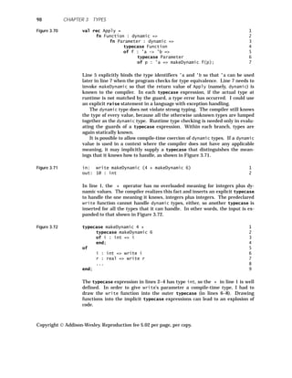
![99
It is much better to coerce at runtime, when the actual type is known for
each dynamic type. The program in Figure 3.72 would clearly use integer ad-
dition and printing of integers. Runtime coercion is still perfectly type-safe,
although some type errors won’t be discovered until runtime.
11 ◆ FINAL COMMENTS
The discussion of derived types and dimensions is part of a larger issue about
how restrictive a programming language needs to be in order to permit the
art of programming. One way to look at this question [Gauthier 92] is to no-
tice that on the one hand the real world is very restrictively typed, as stu-
dents of physics realize. One should not add apples and oranges, much less
volts and calories. On the other hand, the memory of most computers is com-
pletely untyped; everything is represented by bits (organized into equally un-
typed bytes or words). The programming language represents a platform for
describing the real world via the computer, so it properly lies somewhere be-
tween these extremes. It needs to balance type security with simplicity. Type
security demands that each different kind of value have its own type in order
to match the real world. For example, lists of exactly three elements are dif-
ferent from lists of four elements. Integers constrained to even numbers are
different from unconstrained integers. Simplicity demands that types be easy
to specify and that types be efficiently checked, preferably at compile time. It
is not so easy to include lengths or number-theoretic considerations in the
type description of lists and integers, respectively.
It is largely a matter of personal taste where this platform should be on
the spectrum ranging from restrictively typed, using strong typing and per-
haps providing derived types with dimensions, to lax, with dynamic typing
and easy coercion. Proponents of the restrictive style point with pride to the
clarity of their programs and the fact that sometimes they run correctly the
first time. Proponents of the lax style speak disparagingly of “bondage-and-
discipline” languages like Ada, and prefer the relative freedom of C.
Such taste is likely to change as a programmer changes. My first experi-
ence of programming (after plug-board computers) was in machine language,
not even assembler language. Later, I relished the intricacies of SNOBOL,
which is quite lax about typing. Algol was a real eye-opener, with its declared
types and its control structures. I now prefer strong typing; to me, an elegant
program is one that is readable the first time by a novice, not one that plays
unexpected tricks. Strong typing helps me to build such programs. Still, I
use C heavily because it is implemented so widely, and I often need to port my
programs across machines.
ML is an elegant language that shows how to make functions first-class
values and how to deal with type polymorphism and still be strongly typed.
Type inference relieves the programmer of careful type declarations. Mi-
randa extends these ideas with infinite lists and lazy evaluation. (There is
also a lazy variant of ML with similar extensions.) Russell even allows some
types to be manipulated in fairly simple ways. None of these languages truly
allows types themselves to be first-class values. Such an extension would
probably require runtime type checking or lose strong typing. (The exercises
explore this concept.)
Copyright Addison-Wesley. Reproduction fee $.02 per page, per copy.
11 FINAL COMMENTS](https://image.slidesharecdn.com/advancedprogramminglanguagedesign-230706034617-464d64c2/85/Advanced_programming_language_design-pdf-107-320.jpg)
![Type systems are an area of active research. Integrating dimensions into
polymorphic languages like ML, for example, is being studied [Kennedy 94].
The SML variant of ML includes an experimental, higher-order extension of
the module system, in which generic modules can be parameterized by other
(possibly generic) modules.
Although I have intentionally avoided issues of syntax in this chapter, I
would like to point out that syntactic design certainly affects the ease with
which programmers can learn and use a language. Compare, for example,
identical types in C and ML:
C ML
int z z : int
int (*a)(char) a : (char -> int) ref
int (*((*b)(int)))(char) b : (int -> ((char -> int) ref))) ref
int (*c)(int (*)(char)) c : ((char -> int) ref -> int) ref
Although the C type expressions are shorter, I find them difficult to generate
and to understand.
EXERCISES
Review Exercises
3.1 What is the difference between the way Modula-2+ and Modula-3 han-
dle type equivalence for derived types?
3.2 If two types are name-equivalent, are they necessarily structurally
equivalent?
3.3 Would you consider First and Second in Figure 3.73 structurally equiv-
alent? Why or why not?
Figure 3.73 type 1
First = 2
record 3
A : integer; 4
B : record 5
B1, B2 : integer; 6
end; 7
end; 8
Second = 9
record 10
A: record 11
A1, A2 : integer; 12
end; 13
B : integer; 14
Copyright Addison-Wesley. Reproduction fee $.02 per page, per copy.
100 CHAPTER 3 TYPES](https://image.slidesharecdn.com/advancedprogramminglanguagedesign-230706034617-464d64c2/85/Advanced_programming_language_design-pdf-108-320.jpg)
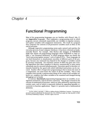
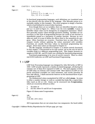
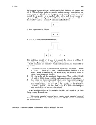
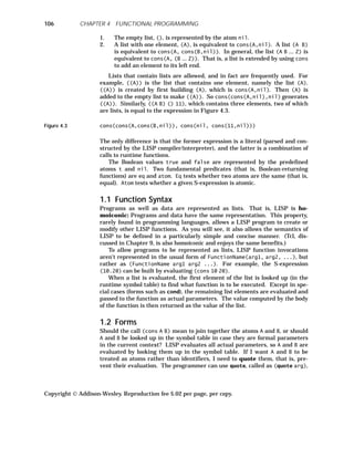
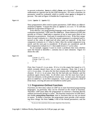
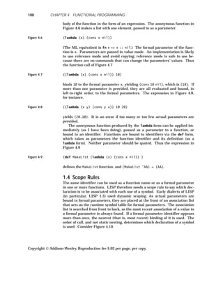
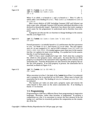
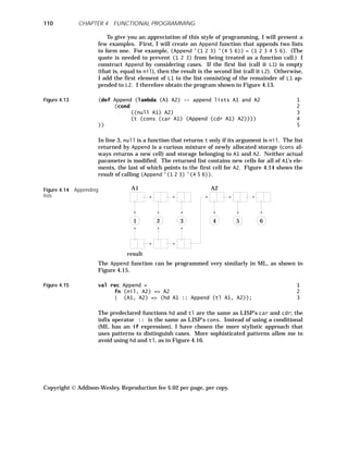
![111
Figure 4.16 val rec Append = 1
fn (nil, A2) => A2 2
| (HA1 :: TA1, A2) => (HA1 :: Append (TA1, A2)); 3
Next, I will build a LISP function that takes a list and returns its reversal.
If the list is empty, the function returns the empty list; otherwise, the first el-
ement of the list will be the last element of the reversed list. I can make this
element into a list (using MakeList defined earlier) then append it to the end
of the reversal of the remainder of the list, arriving at the program shown in
Figure 4.17.
Figure 4.17 (def Reverse (lambda (R) -- reverse list R 1
(cond 2
((null R) R) 3
(t (Append (Reverse (cdr R)) (MakeList (car R)))) 4
) 5
)) 6
The returned list is completely built out of new cons cells. The ML equiva-
lent is given in Figure 4.18.
Figure 4.18 val rec Reverse = 1
fn nil => nil 2
| H :: T => Append(Reverse(T), [H]); 3
As you can see, ML’s ability to build formal parameters that correspond to
components of the actual parameters and its syntax for list construction ([H]
in line 3) give it a different feel from LISP, even though the underlying algo-
rithm is identical.
Reverse only reverses the top-level elements of a list; if the elements are
themselves lists, the lower-level lists aren’t reversed. For example, (Reverse
’(1 (2 3 4) 5))) = (5 (2 3 4) 1). I can define a related function, ReverseAll,
that reverses all lists, even if they appear as elements of another list; thus,
(ReverseAll ’(1 (2 3 4) 5)) = (5 (4 3 2) 1). First, I define the reversal of
any atom (including nil) as equal to that atom itself. Now when I append the
car of a list onto the end of the reversal of the remainder of the list, I make
sure to reverse the car first; thus, I have the code shown in Figure 4.19.
Figure 4.19 (def ReverseAll (lambda (RA) -- reverse RA and sublists 1
(cond 2
((atom RA) RA) 3
(t (Append 4
(ReverseAll (cdr RA)) 5
(MakeList (ReverseAll (car RA)) )))) 6
)) 7
This example cannot be directly translated into ML, because ML’s type
scheme requires that lists be homogeneous. A programmer can, however, in-
troduce a new ML datatype for nonhomogeneous lists; this idea is pursued in
Exercise 4.13.
Copyright Addison-Wesley. Reproduction fee $.02 per page, per copy.
1 LISP](https://image.slidesharecdn.com/advancedprogramminglanguagedesign-230706034617-464d64c2/85/Advanced_programming_language_design-pdf-119-320.jpg)
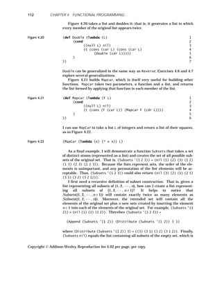
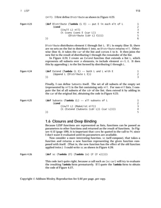
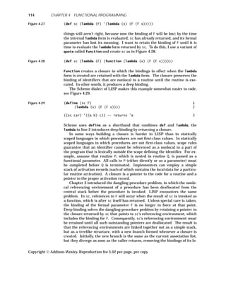
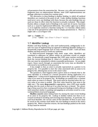
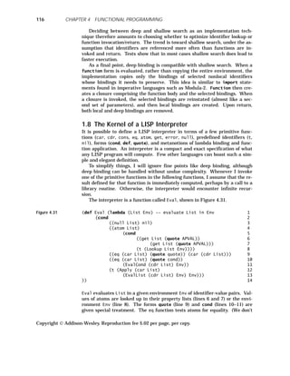
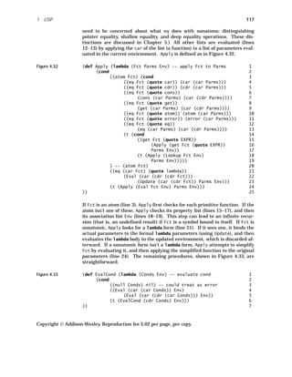
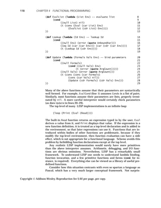
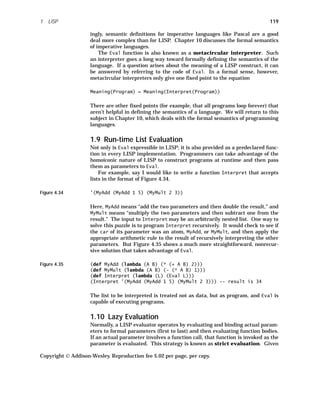
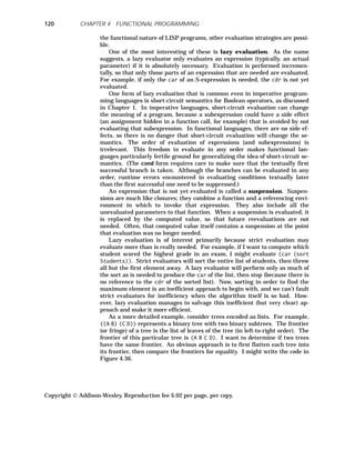
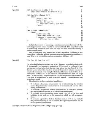
![Let me trace how a lazy evaluator might evaluate
(SameFrontier ’((A B) C) ’(B C (A D))) .
The trace in Figure 4.38 shows the evaluation steps.
Figure 4.38 Goal = (SameFrontier S1=’((A B) C) S2=’(B C (A D))) 1
=[S body] (EqualList E1=(Flatten S1) E2=(Flatten S2)) 2
=[E body] (cond ((null E1) .. ) .. ) .. ) 3
| E1 = (Flatten F1=S1) 4
| =[F body] (cond ((null S1) .. ) .. ) 5
| [S1 is neither null nor an atom] 6
| = (Append A1=(Flatten (car F1)) 7
| A2=(Flatten (cdr F1))) 8
| =[A body] (cond ((null A1) .. ) .. ) 9
| | A1 = (Flatten F2=(car F1)) 10
| | =[F body] (cond ((null F2) .. ) .. ) 11
| | | F2 = (car F1) = (car S1) = (car ’((A B) C)) 12
| | | = ’(A B) 13
| | [F2 is neither null nor an atom] 14
| | A1 = (Append A3=(Flatten (car F2)) 15
| | A4=(Flatten (cdr F2))) 16
| | =[A body] (cond ((null A3) .. ) .. ) 17
| | | A3 = (Flatten F3=(car F2)) 18
| | | =[F body] (cond ((null F3) .. ) .. ) 19
| | | | F3 = (car F2) = (car ’(A B)) = ’A 20
| | | [F3 is not null, but it is an atom] 21
| | | A3 = (MakeList F3) =[M body] (cons F3 nil) 22
| | | = ’(A) 23
| | [A3 is not null] 24
| | A1 = (cons (car A3) (Append (cdr A3) A4)) 25
| [A1 is not null] 26
| E1 = (cons (car A1) (Append (cdr A1) A2)) 27
[E1 is not null] 28
Goal = (cond ((null E2) .. ) .. ) 29
| E2 = (Flatten F4=S2) 30
| =[F body] (cond ((null F4) .. ) .. ) 31
| [F4 is not null or an atom] 32
| = (Append A5=(Flatten (car F4)) 33
| A6=(Flatten (cdr F4))) 34
| =[A body] (cond ((null A5) .. ) .. ) 35
| | A5 = (Flatten F5=(car F4)) 36
| | =[F body] (cond ((null F5) .. ) .. ) 37
| | | F5 = (car F4) = (car S2) 38
| | | = (car ’(B C (A D))) = ’B 39
| | [F5 is not null, but it is an atom] 40
| | A5 = (MakeList F5) =[M body] (cons ’B nil) = ’(B) 41
| [A5 is not null] 42
| E2 = (cons (car A5) (Append (cdr A5) A6)) 43
Copyright Addison-Wesley. Reproduction fee $.02 per page, per copy.
122 CHAPTER 4 FUNCTIONAL PROGRAMMING](https://image.slidesharecdn.com/advancedprogramminglanguagedesign-230706034617-464d64c2/85/Advanced_programming_language_design-pdf-130-320.jpg)
![123
[E2 is not null] 44
Goal = (cond ((eq (car E1) (car E2)) .. ) .. ) 45
= (cond ((eq (car A1) (car A5)) .. ) .. ) 46
= (cond ((eq (car A3) ’B) .. ) .. ) 47
= (cond ((eq ’A ’B) .. ) .. ) 48
= (cond (t nil)) 49
= nil -- frontiers are different 50
The notation is concise, but I hope not too clumsy. I show that a formal pa-
rameter is bound to an actual parameter by the notation Formal=Actual, as
in S1=’((A B) C) in line 1. The names of the formal parameters (here, S) start
with the same letter as the name of the function (SameFrontier). I distin-
guish multiple parameters as well as new instances during recursive calls by
numeric suffixes. Simplification steps are marked in various ways. In line 2,
=[S body] means expanding a call by inserting the body of a function, in this
case, SameFrontier. I have used the declaration of Append from Figure 4.13
(page 110) whenever [A body] is mentioned. The ellipsis (..) shows where
evaluation of cond pauses in order to evaluate a subexpression. It only evalu-
ates the subexpression to the point that it can answer the condition in ques-
tion. For example, in line 9, it is necessary to discover if A1 is null. By line 25
A1 has been evaluated enough to answer the question, as reported in line 26.
These subordinate evaluations are indented. Line 27 continues the evalua-
tion of E1 started on line 4. It leaves the result in terms of A1 and A2, to be
further evaluated in lines 46–48.
Lazy evaluation is more difficult (and costly) to implement than strict
evaluation. The example shows that it has much of the flavor of coroutines
(see Chapter 2), with control automatically shifting as needed among many
computations in order to advance the computation.
An implementation of LISP might allow the programmer to select lazy
evaluation when desired; any evaluation strategy will produce the same re-
sult so long as the program is written in “pure” LISP. (Some dialects include
imperative facilities, which, as you have seen, can make the evaluation order
significant.) Automatic determination of the preferable evaluation strategy is
an open (and hard) problem.
Lazy evaluation is sometimes called “demand-driven evaluation” because
evaluation is triggered by a demand for a value. We conventionally view a
computation (very roughly) as first obtaining input values, then computing a
result using them, and finally printing that result. Demand-driven evalua-
tion reverses this view. Nothing happens until the evaluator sees a request to
write a result. This request initiates computations, which solicit input val-
ues. If no demand for output is seen, nothing is computed.3
Lazy evaluation also has a declarative, nonprocedural flavor. (Chapter 8
discusses logic programming, which is declarative.) Although LISP is cer-
tainly procedural (both imperative and functional languages are in the larger
category of procedural languages), lazy evaluation makes evaluation optional.
hhhhhhhhhhhhhhhhhhhhhhhhhhhhhhhhhhhh
3
This is similar to a folk myth concerning the benchmarking of an optimizing FORTRAN
compiler. The compiler was presented with a very complex program containing no write state-
ments. It optimized the program by generating no code!
Copyright Addison-Wesley. Reproduction fee $.02 per page, per copy.
1 LISP](https://image.slidesharecdn.com/advancedprogramminglanguagedesign-230706034617-464d64c2/85/Advanced_programming_language_design-pdf-131-320.jpg)
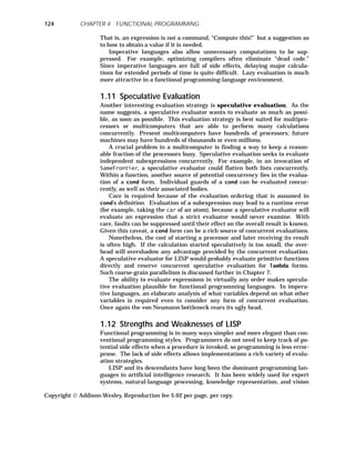
![125
modeling. Only recently has Prolog, discussed in Chapter 8, attracted a sig-
nificant following in these areas. LISP is also the foundation of the widely
used Emacs text editor. Much of LISP’s success is due to its homoiconic na-
ture: A program can construct a data structure that it then executes. The se-
mantics of the core of LISP can be described in just a few pages of a
metacircular interpreter.
LISP was the first language to have an extensive program development
environment [Teitelman 81]. (Smalltalk, described in Chapter 5, was the sec-
ond. Such environments are widely available now for Ada, Pascal, and C++.)
Programs can be modified and extended by changing one function at a time
and then seeing what happens. This facility allows elaborate programs to
evolve and supports rapid prototyping, in which a working prototype is used
to evaluate the capabilities of a program. Later, the program is fleshed out by
completing its implementation and refining critical routines.
The most apparent weakness of the early dialects of LISP is their lack of
program and data structures. In LISP 1.5, there are no type-declaration fa-
cilities (although some LISP dialects have adopted facilities for data typing).
Certainly not everything fits LISP’s recursive, list-oriented view of the world.
For example, symbol tables are rarely implemented as lists.
Many LISP programmers view type checking as something that ought to
be done after a program is developed. In effect, type checking screens a pro-
gram for inconsistencies that may lead to runtime errors. In LISP, type
checking amounts generally to checking for appropriate structures in S-
expressions.
Most production LISP dialects (such as Interlisp, Franz LISP, Common
LISP, and Scheme) have greatly extended the spartan facilities provided in
LISP 1.5, leading to incompatibilities among LISP implementations. Indeed,
it is rare to transport large LISP programs between different implementa-
tions. This failure inhibits the interchange of software tools and research de-
velopments.
It would appear that the corrupting influences of von Neumann program-
ming are so pervasive that even functional languages like LISP can succumb.
Most LISP implementations even have a prog feature that allows an impera-
tive programming style! In addition, LISP has some decidedly nonfunctional
features, such as the set function and property lists. In fact, it has been said
that ‘‘LISP . . . is not a functional language at all. [The] success of LISP set
back the development of a properly functional style of programming by at
least ten years.’’ [Turner 85b]
2 ◆ FP
In comparison to typical block-structured languages, LISP 1.5 stands as a
paragon of simplicity. (On the other hand, Common LISP is as big as Ada.)
Nonetheless, Backus suggests that even simpler functional programming ap-
proaches may be desirable [Backus 78]. He thinks that LISP’s parameter-
binding and substitution rules are unnecessary and instead proposes a vari-
able-free programming style limited to single-parameter functions. (A pa-
rameter may, however, be a sequence, and functions may be curried.)
Further, LISP’s ability to combine functions in any form (since functions are
just S-expressions) is unnecessarily general. He compares this freedom to the
Copyright Addison-Wesley. Reproduction fee $.02 per page, per copy.
2 FP](https://image.slidesharecdn.com/advancedprogramminglanguagedesign-230706034617-464d64c2/85/Advanced_programming_language_design-pdf-133-320.jpg)
![unrestricted use of goto statements in low-level imperative languages. In
contrast, Backus prefers a fixed set of higher-order functions that allow func-
tions to be combined in various ways, analogous to the fixed set of control
structures found in modern imperative languages. The result is the FP pro-
gramming language.
2.1 Definition of an FP Environment
An FP environment comprises the following:
1. A set of objects. An object is either an atom or a sequence, <x1 , . . . , xn
>, whose elements are objects, or ⊥ (“bottom”) representing “error,” or
“undefined.” Included as atoms are φ, the empty sequence (roughly
equivalent to nil in LISP), and T and F, representing true and false.
Any sequence containing ⊥ is equivalent to ⊥. That is, the sequence
constructor is bottom-preserving.
2. A set of functions (which are not objects) mapping objects into objects.
Functions may be primitive (predefined), defined (represented by a
name), or higher-order (a combination of functions and objects using a
predefined higher-order function). All functions are bottom-preserving;
f applied to ⊥ always yields ⊥.
3. An application operation that applies a function to an object, yielding an
object. Function f applied to object x is denoted as f:x. Here, x isn’t a
variable name (there are no variables!), but rather a placeholder for an
expression that will yield an object.
4. A set of higher-order functions used to combine existing functions and
objects into new functions. Typical higher-order functions include those
shown in Figure 4.39.
Figure 4.39 Composition 1
(f ° g):x ≡ f:(g:x) 2
Construction 3
[f1 , ... , fn ]:x ≡ <f1:x, ... ,fn:x> 4
Condition 5
(p → f;g):x ≡ 6
if p:x = T then 7
f:x 8
elsif p:x = F then 9
g:x 10
else 11
⊥ 12
The conditional form handles nicely a problem that arises with bottom-
preserving functions: One or the other branch of a conditional may be
undefined (bottom) while the value of the conditional is itself well de-
fined. If one tries to create a conditional function that takes a triple
representing the Boolean value, the true-part value and the false-part
value, then if any component is ⊥, so is the entire triple, forcing ⊥ as the
result. Since conditional is a higher-order function, the evaluator
doesn’t apply the “then function” or “else function” until the conditional
Copyright Addison-Wesley. Reproduction fee $.02 per page, per copy.
126 CHAPTER 4 FUNCTIONAL PROGRAMMING](https://image.slidesharecdn.com/advancedprogramminglanguagedesign-230706034617-464d64c2/85/Advanced_programming_language_design-pdf-134-320.jpg)
![127
value has been evaluated and tested against T and F.
One of the advantages of restricting higher-order functions is that
they form an algebra, which allows forms to be manipulated in well-
defined ways. For example, Figure 4.40 is a theorem:
Figure 4.40 [f1 , ... ,fn ] ° g ≡ [f1 ° g, ... , fn ° g]
This theorem states that a composed function may be “distributed into”
or “factored from” a list of functions. Such algebraic theorems can be
viewed as the basis for automatic restructuring of FP programs, poten-
tially allowing sophisticated optimizations.
5. A set of definitions binding functions to identifiers. These identifiers
serve merely as abbreviations and placeholders; there is no concept of
redefinition or scoping.
2.2 Reduction Semantics
FP environments have a particularly simple semantics called reduction se-
mantics. An FP program is composed of a number of functions applied to ob-
jects. The meaning of such a program is defined by repeatedly reducing the
program by finding a function application and evaluating it. In some cases,
function evaluation may be nonterminating. Such functions diverge and are
considered undefined (that is, ⊥). There are only three kinds of valid func-
tions: primitive functions, defined functions, and higher-order functions.
Primitive functions are automatically evaluable. Defined functions are re-
duced by replacing their identifiers with their definitions. Higher-order func-
tions are reduced by substituting their definitions. If a function does not
belong to one of these three categories, it is invalid.
Reduction semantics have only a very weak form of identifier binding (de-
fined names map to functions) and employ no changes to hidden states.
There is clearly no way to cause side effects, so an evaluator can reduce a
function in any order. In fact, early FP languages were called “Red” (reduc-
tion) languages.
3 ◆ PERSISTENCE IN FUNCTIONAL LANGUAGES
A value is persistent if it is retained after the program that created it has
terminated. A database is a good example of persistent values. The conven-
tional way to make values persistent is to write them out to a file. Chapter 3
discusses the type-safety considerations of such values.
If persistent values are to be incorporated into a programming language,
we must be able to name such values and to be assured that once created,
they do not change. Functional languages can incorporate persistent values
in a natural way that avoids explicit input and output [Morrison 90].
Persistent values can be named by reference to a persistence root,
which is something like the root of a file-system hierarchy. All such values
are automatically saved after execution. If a value is structured, its compo-
nents are also preserved; in particular, other values pointed to by a persistent
value are also persistent. Using ML as an example, we might have the code
Copyright Addison-Wesley. Reproduction fee $.02 per page, per copy.
3 PERSISTENCE IN FUNCTIONAL LANGUAGES](https://image.slidesharecdn.com/advancedprogramminglanguagedesign-230706034617-464d64c2/85/Advanced_programming_language_design-pdf-135-320.jpg)
![shown in Figure 4.41.
Figure 4.41 let 1
val persist(MyRoot) a.b.c = 3; 2
val persist(MyRoot) d.e; 3
in 4
a.b.c + d.e 5
end; 6
Here, the identifier a.b.c is introduced as persistent, under root MyRoot, and
is given the (permanent) value 3. The identifier d.e is not given a value; in-
stead, it gets its value from persistent storage, where it should already be de-
fined.
Since functional languages have no side effects, persistent values are im-
mutable, so there is no need to worry about getting consistent copies if two
programs access the values at the same time: such values cannot change. It
would be a runtime error to reintroduce the same identifier in a persistence
hierarchy. The only modification allowed is inserting an object into (and per-
haps removing an object from) the persistent store.
The possibility of lazy evaluation in functional programming languages
make them even more attractive for persistent store. An incompletely evalu-
ated value, that is, a suspension, can be saved in persistent store so long as
the environment on which it depends is also treated as persistent. If later
computation resolves, fully or partially, the suspension, it is safe to replace
the stored suspension with the resolved value. Future evaluations, either by
the same program or by other programs, will see effectively the same values.
One proposal for integrating persistence into a functional language is to
build an imperative command outside the language (at the operating-system
level, for example) [McNally 91]. The expression in Figure 4.42
Figure 4.42 persist ModuleA requires ModuleB, ModuleC
means that all identifiers exported from ModulaA are to be placed in persis-
tent store. Both ModuleB and ModuleC must already be in persistent store;
values in ModuleA may depend on them. If ModuleA is already in persistent
store, the new copy replaces it, but any pointers to the identifiers of the previ-
ous ModuleA are still valid. The old ModuleA becomes collectable; that is,
garbage collection routines may discard and reclaim the storage of any of its
values that are no longer pointed to.
4 ◆ LIMITATIONS OF FUNCTIONAL
LANGUAGES
The idea that variables are unnecessary is quite attractive. It is often suffi-
cient either to bind values through parameter binding or as constants for the
duration of a block. For example, in ML, the let construct allows an identi-
fier to be bound to a meaning, but there is no assignment as such. There are
situations, however, in which the inability to modify an existing value leads to
awkward or inefficient programs [Arvind 89; Yuen 91].
Copyright Addison-Wesley. Reproduction fee $.02 per page, per copy.
128 CHAPTER 4 FUNCTIONAL PROGRAMMING](https://image.slidesharecdn.com/advancedprogramminglanguagedesign-230706034617-464d64c2/85/Advanced_programming_language_design-pdf-136-320.jpg)
![129
The first problem involves initializing complex data structures, particu-
larly two-dimensional arrays. For example, I might want an array A with the
properties shown in Figure 4.43.
Figure 4.43 A[0,j] = A[i, 0] = 1 ∀ 0 ≤ i < n, 0 ≤ j < n 1
A[i,j] = A[i, j-1] + A[i-1, j] + A[i-1, j-1] 2
∀ 0 < i < n, 0 < j < n 3
Short of embedding syntax for this elegant mathematical declaration into a
programming language, the most straightforward way to accomplish this ini-
tialization is with an imperative program that iterates as in Figure 4.44.
Figure 4.44 variable 1
sum, row, col : integer; 2
A : array [0..n-1, 0..n-1] of integer; 3
begin 4
for sum := 0 to 2*n-2 do 5
for row := max(0,sum-n+1) to min(n-1,sum) do 6
col := sum - row; 7
if row = 0 or col = 0 then 8
A[row, col] := 1 9
else 10
A[row,col] := A[row, col-1] + 11
A[row-1, col] + A[row-1, col-1] 12
end; 13
end; -- for row 14
end; -- for sum 15
end; 16
In a functional language, initialization is usually performed by recursion,
which returns the value that is to be associated with the identifier. But there
is no obvious recursive method that works here, for several reasons. First,
unlike lists, arrays are not generally built up by constructors acting on pieces.
The entire array is built at once.4
Second, the natural initialization order,
which is by a diagonal wavefront, does not lend itself either to generating
rows or columns independently and then combining them to make the array.
Third, special-purpose predeclared array constructor functions can only han-
dle simpler cases in which the value at each cell depends only on the cell’s in-
dices. For example, to build an array in which each cell has a value computed
as the sum of its row and column, we could employ such a function and in-
voke it as MakeArray(1, n, 1, n, (fn row, col => row+col)). That approach
fails here, because the value in a cell depends on other values within the ar-
ray.
One solution to this problem that largely preserves referential trans-
parency, that is, that references to an identifier should always produce the
same results, is to separate allocation of data from initialization. After the
array is built, a language could permit individual cells to be assigned values,
hhhhhhhhhhhhhhhhhhhhhhhhhhhhhhhhhhhh
4
APL, discussed in Chapter 9, allows arrays to be built piecemeal.
Copyright Addison-Wesley. Reproduction fee $.02 per page, per copy.
4 LIMITATIONS OF FUNCTIONAL LANGUAGES](https://image.slidesharecdn.com/advancedprogramminglanguagedesign-230706034617-464d64c2/85/Advanced_programming_language_design-pdf-137-320.jpg)
![but only once each. Accesses to values that have not been initialized would be
erroneous. (In concurrent programming, discussed in Chapter 7, such ac-
cesses would block the thread that tries to access such a cell until the cell is
initialized.) Unfortunately, this solution requires that the language have as-
signment and that there be runtime checks for violations of the single-
assignment rule.
Initialized identifiers are not the only problem with functional languages.
A different problem arises if I want to summarize information in counters.
For example, I may have a function that returns values from 1 to 10, and I
want to invoke the function a million times with different parameters. I want
to know how often each of the possible return values appears. In an impera-
tive language, it is quite easy to store such results in an array that is initially
0 everywhere and updated after each function invocation. In a functional lan-
guage, there seems to be no alternative but to enter a new name scope after
each function call, getting a new array that is initialized to the old one except
for one position, where it is incremented. The only reasonable way to enter a
million name scopes is by recursion, and even that seems problematic. A so-
lution to the problem of summarizing information in a functional language is
found in the guardians in Post (discussed in Chapter 6) and in multiparadigm
languages like G-2.
Finally, functional languages sometimes lose nuances that are essential to
efficiency. For example, the Quicksort algorithm can be expressed elegantly
in Miranda (Chapter 3) as in Figure 4.45.
Figure 4.45 fun 1
QuickSort [] = [] 2
QuickSort (a :: rest) = 3
QuickSort [ b | b <- rest; b <= a ] @ 4
[a] @ 5
QuickSort [ b | b <- rest; b > a]; 6
However, this representation misses some important details. First, it is inef-
ficient to make two passes through the array to partition it into small and
large elements. Second, stack space can be conserved by recursing on the
smaller sublist, not always the first sublist (I assume the compiler is smart
enough to replace the tail recursion with iteration). Third, Quicksort should
sort elements in place; this implementation builds a new array. The first two
details can be programmed in the functional model, although perhaps awk-
wardly. The other is too intricately associated with concepts of swapping val-
ues in memory locations.
Copyright Addison-Wesley. Reproduction fee $.02 per page, per copy.
130 CHAPTER 4 FUNCTIONAL PROGRAMMING](https://image.slidesharecdn.com/advancedprogramminglanguagedesign-230706034617-464d64c2/85/Advanced_programming_language_design-pdf-138-320.jpg)
![131
5 ◆ LAMBDA CALCULUS
The mathematician Alonzo Church designed the lambda calculus in the 1930s
as a way to express computation [Church 41]. LISP is a direct descendent of
this formalism, and ML owes much of its nature to a restricted version called
“typed lambda calculus.” In one sense, lambda calculus is a set of rules for
manipulating symbols; the symbols represent functions, parameters, and in-
vocations. In another sense, lambda calculus is a programming language; it
has given rise more or less directly to both LISP and ML.
The underlying ideas of lambda calculus are straightforward. Lambda
calculus has only three kinds of terms: identifiers (such as x), abstractions,
and applications. Abstractions represent functions of a single parameter.
They follow the notation shown in Figure 4.46.
Figure 4.46 (λ x . (* x 2)) -- Lambda calculus 1
(lambda (x) (* x 2)) -- LISP 2
fn x => x * 2 -- ML 3
In general, an abstraction has the form (λ x . T), where T is any term. Ap-
plications represent invoking a function with an actual parameter. A func-
tion F is invoked with actual parameter P by the notation (F P); both F and P
are any terms. Parentheses may be dropped; the precedence rules stipulate
that application and abstraction are grouped left to right and that application
has a higher precedence than abstraction. Therefore, the terms in Figure
4.47 are equivalent.
Figure 4.47 (λ x . ((λ y . q) x) z) -- fully parenthesized 1
λ x . (λ y . q) x z -- minimally parenthesized 2
Another notational convenience is that curried functions may be rewritten
without currying, as in Figure 4.48.
Figure 4.48 (λ x . (λ y . (λ z . T))) = (λ x y z . T)
Lambda calculus has a static scope rule. The abstraction (λ x . T) intro-
duces a new binding for the identifier x; the scope of this binding is the term
T. In the language of lambda calculus, x is bound in (λ x . T). An unbound
identifier in a term is called free in that term. It is possible to define the con-
cept of free identifiers in a recursive way: An identifier x is free in term T if
(1) the term is just the identifier x; (2) the term is an application (F P), and x
is free in F or in P; or (3) the term is an abstraction (λ y . T), and x is free in
T, and x is not y. Figure 4.49 presents some examples.
Copyright Addison-Wesley. Reproduction fee $.02 per page, per copy.
5 LAMBDA CALCULUS](https://image.slidesharecdn.com/advancedprogramminglanguagedesign-230706034617-464d64c2/85/Advanced_programming_language_design-pdf-139-320.jpg)
![Figure 4.49 (λ x . y) (λ y . z) -- y and z are free; x is bound 1
(λ x . y) (y z) -- y and z are free; x is bound 2
(λ y . (y z)) -- z is free; y is bound 3
(λ x . (λ y . z)) -- z is free; x and y are bound 4
(λ x . (λ x . z)) -- z is free; x is bound 5
The example in line 5 introduces two different bindings for x. This situation
is analogous to an inner declaration that conflicts with an outer declaration.
As you expect, the meaning of x within any term is based on the closest en-
closing binding. The rules of lambda calculus, which you will see shortly, en-
sure that this interpretation is followed.
The heart of lambda calculus is the rule of Figure 4.50 that lets you sim-
plify a term.
Figure 4.50 (λ x . T) P =β=> {P / x} T
This formula says that applying a function (λ x . T) to an actual parameter P
yields the body T of the function, with all occurrences of the formal parameter
x replaced by the actual parameter P. This simplification is called β (beta)
reduction, and I denote it by the symbol =β=> . The notation {P / x} T can
be read as “P instead of x in T”. It is somewhat awkward to define this substi-
tution operator precisely. First, x may have bound occurrences in T that
should not be subject to substitution. These are like nested declarations of x,
which hide the outer declaration that we are trying to bind to P. Second, P
may have unbound instances of identifiers that are bound in T. These identi-
fiers must remain unbound in the substitution. To achieve this goal, such
identifiers need to be renamed in T before substitution takes place. Figure
4.51 shows some examples of substitution.
Figure 4.51 {a / b} b = a -- no renaming needed
{a / b} a = a -- no free instances of b
{a / b} (λ c . b) = (λ c . a) -- no renaming needed
{a / b} (λ b . b) = (λ z . z) -- b=>z; no free instances left
{a / b} ((λ b . b)(b c)) = (λ z . z)(a c) -- renamed bound b=>z
{(λ x . y) / x} (x y) = ((λ x . y) y)
The concept of renaming bound identifiers can be formalized; it is called α
(alpha) conversion (see Figure 4.52).
Figure 4.52 (λ x . T) =α=> (λ y . {y / x} T)
Be aware that α conversion requires that y not be free in T.
Figure 4.53 is a fairly complicated example that uses α-conversions and
β-reductions.5
hhhhhhhhhhhhhhhhhhhhhhhhhhhhhhhhhhhh
5
Modified from [Sethi 89].
Copyright Addison-Wesley. Reproduction fee $.02 per page, per copy.
132 CHAPTER 4 FUNCTIONAL PROGRAMMING](https://image.slidesharecdn.com/advancedprogramminglanguagedesign-230706034617-464d64c2/85/Advanced_programming_language_design-pdf-140-320.jpg)
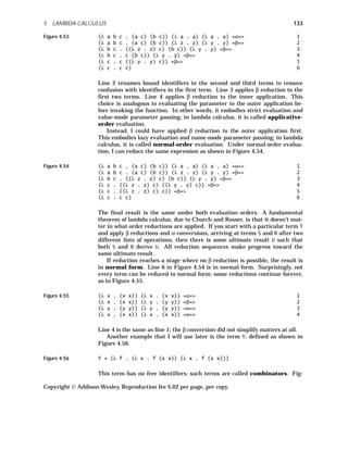
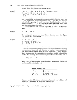
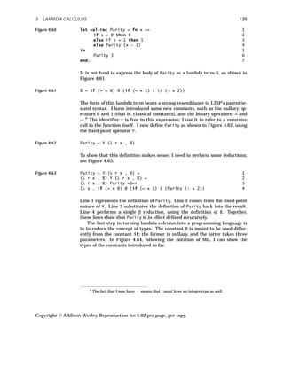
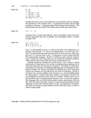
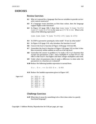
![4.13 As suggested in the text (page 111), show how to use an ML datatype to
implement heterogeneous lists. You may assume that atoms are always
integers or nil. Implement both Reverse and ReverseAll. If you use
:: as a constructor for your list datatype, ML automatically overloads
the [] syntax for you.
4.14 What sort of runtime storage organization is appropriate for ML? Re-
strict your answer to the purely functional part of ML.
4.15 On page 114, I claim that building a closure is easy in statically scoped
languages in which procedures are not first-class values. Is it harder if
procedures are first-class values?
4.16 Does LISP really need garbage collection? Wouldn’t reference counts
suffice?
4.17 On page 116, I suggest that the implementation copy only the bindings
of selected nonlocal identifiers whose bindings it needs to preserve.
How does it know which ones?
4.18 On page 117, I say that the updated environment is discarded after a
lambda body is evaluated. But the example shows no explicit discard.
Explain.
4.19 How must the LISP interpreter be enhanced to deal with deep binding?
4.20 The trace of lazy evaluation in Figure 4.38 (starting on page 122) hap-
pened not to need to return to a partially evaluated result. Trace the
more interesting example
(SameFrontier ’(A B C) ’(A C D)),
which will need to do so.
4.21 In FP, the sequence constructor is bottom-preserving. Show how this re-
quirement precludes lazy evaluation.
4.22 To introduce persistence into a functional language, I have used an im-
perative command. Is an imperative style necessary?
4.23 Use the combinator Y to build a lambda-calculus definition of integer
multiplication that translates the ML program of Figure 4.68.
Figure 4.68 val rec Multiply = fn (x,y) => 1
if x = 0 then 0 else Multiply(x-1,y) + y; 2
4.24 What is the type of Y in Figure 4.56 (page 133)?
4.25 Write a lambda term that grows longer after each β reduction.
Copyright Addison-Wesley. Reproduction fee $.02 per page, per copy.
138 CHAPTER 4 FUNCTIONAL PROGRAMMING](https://image.slidesharecdn.com/advancedprogramminglanguagedesign-230706034617-464d64c2/85/Advanced_programming_language_design-pdf-146-320.jpg)
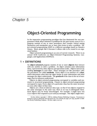
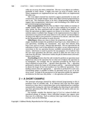
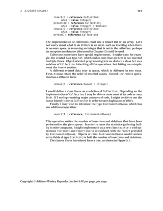
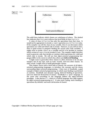
![143
3 ◆ SIMULA
Object-oriented programming began when Simula introduced a novel concept:
A record may contain a procedure field. Such records are called classes.1
As
an example, consider Figure 5.2.
Figure 5.2 class Stack; 1
Size : 0..MaxStackSize := 0; -- initialized 2
Data : array 0..MaxStackSize-1 of integer; 3
procedure Push(readonly What : integer); 4
begin 5
Data[Size] := What; 6
Size := Size+1; 7
end; -- Push; 8
procedure Pop() : integer; 9
begin 10
Size := Size-1; 11
return Data[Size]; 12
end -- Pop; 13
procedure Empty() : Boolean; 14
begin 15
return Size = 0; 16
end; -- Empty 17
end; -- Stack 18
variable 19
S1, S2 : Stack; 20
begin 21
S2 := S1; 22
S1.Push(34); 23
if not S2.Empty() then S2.Pop() end; 24
end; 25
Classes are like types; variables may be declared of a class type, as in line 20.
Each such declaration introduces a new instance of the class, that is, a new
object. The object contains fields that are variables (that is, instance vari-
ables) and fields that are procedures (that is, methods). Object variables can
be assigned (line 22); objects can be manipulated by their methods, which are
named just like fields (lines 23 and 24). The three methods of Stack all have
an implicit parameter: the stack object itself. Therefore, the call in line 23
implicitly acts on stack S1.
A problem with classes is that a binary operation, such as testing two
stacks for equality, must be performed by either the first or the second object,
taking the other object as a parameter, as shown in Figure 5.3.
hhhhhhhhhhhhhhhhhhhhhhhhhhhhhhhhhhhh
1
Simula’s classes are the ancestors of Pascal’s records and coroutines (Chapter 2), in addi-
tion to object-oriented programming.
Copyright Addison-Wesley. Reproduction fee $.02 per page, per copy.
3 SIMULA](https://image.slidesharecdn.com/advancedprogramminglanguagedesign-230706034617-464d64c2/85/Advanced_programming_language_design-pdf-151-320.jpg)
![Figure 5.3 class Stack; 1
Size : 0..MaxStackSize := 0; -- initialized 2
Data : array 0..MaxStackSize-1 of integer; 3
procedure Equal(readonly Other : Stack) : Boolean; 4
begin 5
return Other.Size = Size and 6
Other.Data[0..Other.Size-1] = 7
Data[0..Size-1] -- equality of slices 8
end; -- Equal 9
... -- other procedures as before 10
end; -- Stack 11
variable 12
S1, S2 : Stack; 13
begin 14
if S1.Equal(S2) then ... 15
end; 16
In lines 6–7, fields Size and Data of the implicitly passed Stack have simple
names, but the variables of Other, which is explicitly passed, must be quali-
fied by the object intended. (If needed, the pseudovariable Self may be used
to name the implicit object explicitly.) Invoking the Equal method in line 15
shows how asymmetric the binary operation has become. The same problem
appears in Smalltalk, but is solved in C++, as you will see below.
In this example, I have allowed the Equal method of one object to access
the instance variables of another object of the same class. Object-oriented
languages differ in how much access they permit to instance variables and
how much the programmer can control that access. I will return to this issue
when I discuss C++.
Simula allows new classes to inherit instance variables and methods of old
classes. Subclasses raise the issues of assignment compatibility, overloading
of procedures, and dynamic binding of procedures, all of which are discussed
in detail below.
4 ◆ SMALLTALK
Smalltalk is the name of a family of programming languages developed at Xe-
rox PARC (Palo Alto Research Center) as part of the Dynabook project. Dyn-
abook was envisioned as the ultimate personal computer — small, portable,
with excellent graphics and virtually unlimited memory and computing
power. Smalltalk was designed as Dynabook’s programming language.
Smalltalk has gone through a long evolution, including Smalltalk-72,
Smalltalk-76, Smalltalk-78, and Smalltalk-80. Many individuals have con-
tributed to the development of its variants, most notably Alan Kay, Daniel In-
galls, and Peter Deutsch. I will consider only Smalltalk-80, and whenever I
say “Smalltalk,” I mean Smalltalk-80. A standard Smalltalk reference is
known as the Blue Book [Goldberg 83].
Copyright Addison-Wesley. Reproduction fee $.02 per page, per copy.
144 CHAPTER 5 OBJECT-ORIENTED PROGRAMMING](https://image.slidesharecdn.com/advancedprogramminglanguagedesign-230706034617-464d64c2/85/Advanced_programming_language_design-pdf-152-320.jpg)
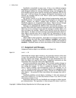
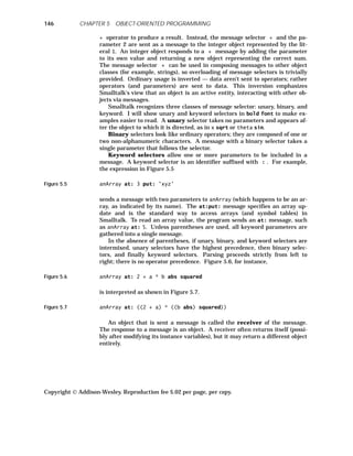
![147
4.2 Blocks
Smalltalk blocks represent a sequence of actions that are encapsulated into a
single object. Blocks are used to implement control structures as well as
functions. A block is a sequence of expressions, separated by periods and de-
limited by square brackets, as shown in Figure 5.8.
Figure 5.8 [index := index + 1. anArray at: index put: 0]
When a block expression is encountered, the statements in the block aren’t
immediately executed. For example, the code in Figure 5.9
Figure 5.9 incr := [index := index + 1. anArray at: index put: 0]
assigns the block to variable incr, but doesn’t perform the addition or array
update. The unary message selector value causes a block to be executed.
Thus incr value will increment index and zero an element of anArray. In
particular, [statement list] value directly executes the anonymous block.
The value returned by a block when it is evaluated is the value returned by
the last statement in the block.
Blocks are used in conditional and iterative constructs in an interesting
manner. Consider an if statement, which is coded in Smalltalk, by sending
two blocks (one for each branch) to a Boolean value, which selects the appro-
priate block and then executes it, as in Figure 5.10.
Figure 5.10 a < 0 1
ifTrue: [b := 0] 2
ifFalse: [b := a sqrt] 3
Our usual model of conditional statements has been inverted. A Boolean
value isn’t passed to an if statement; rather the if statement is passed to the
Boolean!
Repetitive execution is obtained by passing a loop body to an integer or to
a Boolean block, as in Figure 5.11.
Figure 5.11 4 timesRepeat: [x := x sin] 1
[a < b] whileTrue: [b := b sqrt] 2
The Boolean value a < b is enclosed in a block in line 2. The whileTrue: mes-
sage is only understood by blocks, not by Booleans. The reason for this design
is that the block can be reevaluated after each iteration, eventually resulting
in False and terminating the loop. A Boolean value is immutable, so it is
worthless for loop control.
Blocks can also take parameters and be used as functions. Block parame-
ters are prefixed with : and are separated from the block body by | , as in
Figure 5.12.
Copyright Addison-Wesley. Reproduction fee $.02 per page, per copy.
4 SMALLTALK](https://image.slidesharecdn.com/advancedprogramminglanguagedesign-230706034617-464d64c2/85/Advanced_programming_language_design-pdf-155-320.jpg)
![Figure 5.12 [:elem | elem sqrt]
Parameters can be supplied by using one or more value: keyword selectors,
as in Figure 5.13.
Figure 5.13 [:elem | elem sqrt] value: 10 -- 10 sqrt
Anonymous blocks with parameters are handy for applying a function to an
array of elements. The keyword selector collect: creates an array by apply-
ing a block to each element of an array, as in Figure 5.14.
Figure 5.14 #(1 2 3 4) collect: [:elem | elem sqrt] 1
-- (1 1.414 1.732 2) 2
4.3 Classes and Methods
Since all objects are instances of classes, the properties of an object are de-
fined in its class definition. A class contains instance variables (each instance
of the class contains an instance of each of these variables) and instance
methods (each instance of the class responds to messages that invoke these
methods). Instance variables have values that are private to a single object.
Syntax rules require that instance variables begin with a lowercase letter.
(Uppercase letters are only used for shared variables, visible globally, such
as Object.)
Classes are themselves objects, and therefore are members (instances) of
some other class. For example, Integer belongs to Integer class. Integer
class is called a metaclass. All metaclasses belong to class Metaclass,
which is the only instance of Metaclass class, which is itself an instance of
Metaclass.
A new instance of a class is created by sending the message new to the cor-
responding class. Thus the code in Figure 5.15
Figure 5.15 anArray := Array new: 4
would create a new array object with 4 cells (each initialized to nil) and as-
sign it to anArray.
Programming languages that support abstract data types (and a class is a
glorified abstract data type) often allow the programmer to separate the de-
scription of a type (here, class) into a specification and implementation part.
Smalltalk does not let the programmer separate specification from implemen-
tation cleanly, but it does provide much of what you would expect from ab-
stract data types, particularly information hiding.
Figure 5.16 shows how to declare the abstract data type Stack.
Copyright Addison-Wesley. Reproduction fee $.02 per page, per copy.
148 CHAPTER 5 OBJECT-ORIENTED PROGRAMMING](https://image.slidesharecdn.com/advancedprogramminglanguagedesign-230706034617-464d64c2/85/Advanced_programming_language_design-pdf-156-320.jpg)
![149
Figure 5.16 Object subclass: #Stack 1
instanceVariableNames: ’count elements’ 2
classVariableNames: ’MaxDepth’ 3
poolDictionaries: ’’ 4
category: ’Example’ 5
! 6
!Stack class methodsFor: ’creation’! 7
initialize -- sets default depth 8
MaxDepth := 100 9
! 10
new -- builds a new stack of default depth 11
ˆ super new init: MaxDepth 12
! 13
new: desiredDepth -- builds new stack of given depth 14
ˆ super new init: desiredDepth 15
! ! 16
!Stack methodsFor: ’initialization’! 17
init: depth 18
count := 0. 19
elements := Array new: depth 20
! ! 21
!Stack methodsFor: ’access’! 22
empty 23
ˆ count = 0 24
! 25
push: elem 26
count >= elements size 27
ifTrue: [self error: ’Stack overflow’] 28
ifFalse: [ 29
count := count + 1. elements at: count put: elem] 30
! 31
pop |top| 32
self empty 33
ifTrue: [self error: ’Stack is empty’] 34
ifFalse: [ 35
top := elements at: count. 36
count := count - 1. 37
ˆ top 38
] 39
! ! 40
The definition of a class first specifies its name (line 1), the names of the in-
stance variables (line 2), and some other things (lines 3− 6). For the stack ex-
ample, the instance variables are count and elements, the first an integer
counting how many elements are in the stack, and the second an array hold-
ing the stack items. Since Smalltalk is dynamically typed, these declarations
do not indicate any type.
Stack is a subclass of the class Object. You will see the implications of
subclasses later; for now, it suffices that class Object will respond to a mes-
sage of type subclass:instanceVariableNames:...category: and build a
Copyright Addison-Wesley. Reproduction fee $.02 per page, per copy.
4 SMALLTALK](https://image.slidesharecdn.com/advancedprogramminglanguagedesign-230706034617-464d64c2/85/Advanced_programming_language_design-pdf-157-320.jpg)
![Figure 5.17 Stack subclass: #IntegerStack 1
instanceVariableNames: ’’ 2
classVariableNames: ’’ 3
poolDictionaries: ’’ 4
category: ’Example’ 5
! 6
!IntegerStack methodsFor: ’access’! 7
push: elem 8
count >= elements size 9
ifTrue: [self error: ’Stack overflow’] 10
ifFalse: [ 11
elem class = Integer 12
ifTrue: [ 13
count := count + 1. 14
elements at: count put: elem 15
] 16
ifFalse: [self error: ’Can only push integers.’] 17
] 18
! 19
+ aStack |answer i| 20
(self currentDepth) = (aStack currentDepth) 21
ifFalse: [self error: 22
’Incompatible stacks for addition’] 23
ifTrue: [ 24
answer := IntegerStack init: (elements size). 25
i := 1. 26
self currentDepth timesRepeat: [ 27
answer push: 28
(elements at: i) + (aStack pos: i). 29
i := i + 1 30
]. 31
ˆ answer 32
] 33
! ! 34
pos: i -- a private method 35
ˆ elements at: i 36
! 37
currentDepth -- a private method 38
ˆ count 39
! 40
In line 12, the push: method checks that the class of the element about to be
pushed is, in fact, Integer. All objects answer the message class with the
class of which they are an instance. They inherit this ability from Object.
The class hierarchy based on the subclass relation is quite extensive. Fig-
ure 5.18 shows a part of the hierarchy.
Copyright Addison-Wesley. Reproduction fee $.02 per page, per copy.
152 CHAPTER 5 OBJECT-ORIENTED PROGRAMMING](https://image.slidesharecdn.com/advancedprogramminglanguagedesign-230706034617-464d64c2/85/Advanced_programming_language_design-pdf-160-320.jpg)
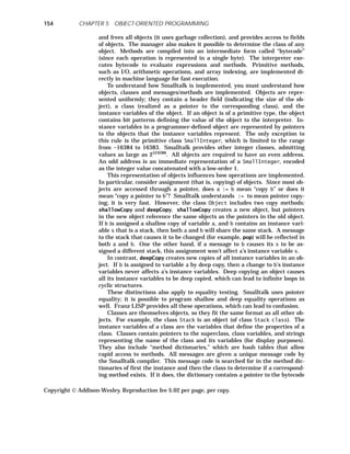
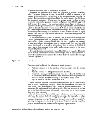
![4.6 Subtle Features
Blocks are implemented by closures. Even though a block may be executed in
an environment quite different from its defining environment, it can still ac-
cess its nonlocal variables correctly. Thus Smalltalk uses deep binding.
Smalltalk manages to avoid the pitfall of accessing deallocated regions of a
stack by using a garbage collector instead of a stack (with its explicit release)
to manage object store. The anonymous method in Figure 5.20 prints 4.
Figure 5.20 |innerBlock outerBlock aVariable| 1
outerBlock := [ :aVariable | 2
innerBlock := [ 3
aVariable write -- write aVariable 4
] 5
] . 6
outerBlock value: 4 . 7
aVariable := 6 . -- Try to confuse the issue 8
innerBlock value -- writes 4 9
! 10
Smalltalk methods are perfectly capable of coercing their parameters; only
by looking at the documentation (or the implementation) can a programmer
be sure what types are accepted by a method and whether the method will co-
erce types.
Even more surprising is the become: method provided by Object (and
therefore available in all classes unless overridden). It is used as in Figure
5.21.
Figure 5.21 anObject become: anotherObject
After this message, all references to anObject and anotherObject are inter-
changed. Conventionally, anotherObject had no references before, so it now
acquires references. This facility can be used to build abstract data types
that change their implementation at some point. That is, in response to some
message, an object may execute the code in Figure 5.22.
Figure 5.22 self become: newObject
From that point on, all references to the old object are rerouted to the new ob-
ject, which could be of a different class entirely.
In many ways tree-structured inheritance rules are too restrictive. For
example, I might have a class DisplayItem that represents items that can be
graphically displayed on a screen. Objects of this class would respond to mes-
sages like rotate: or highlight. Another useful class might be Invento-
ryItem, which represents items that I might inventory. Objects of this class
would respond to messages like reportBacklog or nameSupplier. It would be
nice to allow some objects to be both DisplayItems and InventoryItems (for
example, a bumper or aircraft wing). This can only be done in Smalltalk 1.0
by making DisplayItem a subclass of InventoryItem or vice versa. Neither
alternative is attractive, because not all objects of one class necessarily belong
Copyright Addison-Wesley. Reproduction fee $.02 per page, per copy.
156 CHAPTER 5 OBJECT-ORIENTED PROGRAMMING](https://image.slidesharecdn.com/advancedprogramminglanguagedesign-230706034617-464d64c2/85/Advanced_programming_language_design-pdf-164-320.jpg)
![157
to the other. (For example, I might be able to display a Saturn V rocket, but I
probably won’t have it in my inventory.)
A means of achieving multiple inheritance, in which a class is a direct
subclass of more than one superclass, was introduced in Smalltalk 2.0. It is
complicated to use (none of the built-in Smalltalk classes uses it), because
there can be name conflicts among the multiple ancestral lines. Smalltalk 2.0
notices such conflicts at runtime and declares a conflict error. Since all
classes are subclasses of Object, a class that inherits multiply sees Object
along two different ancestry lines. The programmer needs to indicate
whether such multiply defined ancestors are to be treated as a single ancestor
or whether both are wanted. In the latter case, every invocation of a multiply
defined method or access to a multiply defined instance variable must be
qualified to indicate which ancestor is meant. In Eiffel, the programmer may
rename inherited identifiers to avoid such name conflicts. Circular inheri-
tance is always disallowed.
5 ◆ C++
C++ was developed at AT&T by Bjarne Stroustrup, who wanted to write
event-driven simulations for which Simula would have been ideal but would
also have been too inefficient. The original version of the language was devel-
oped in 1980; at that time it was known as “C with Classes” and lacked a
number of its present features. The name C++ was coined by Rick Mascitti in
1983 as a pun on the C operator ++ , which increments its operand. C++ is
explicitly intended as the successor to C. (The same pun has been used to
name [incr Tcl], an object-oriented enhancement to Tcl.) C++ was imple-
mented for some time as a preprocessor that generated C. Full compilers are
now available. C++ has an ANSI standard and a standard reference, the
ARM [Ellis 90], which also includes some of the design rationale. Of particu-
lar interest is Meyers’ book [Meyers 92], which explains how to use some of
the language features and also why C++ does things the way it does.
5.1 The Consequences of Static Binding
Most of the differences between C++ and Smalltalk can be explained by the
fact that C++ is designed to be an efficient, compiled language. It performs as
much binding as possible statically, not dynamically. Unlike Smalltalk, C++
is a statically typed programming language. Every identifier in a C++ pro-
gram has a type associated with it by a declaration. That type can be either
an ordinary C type or a class.
One consequence of static typing is that C++ does not allow classes to be
introduced at runtime, unlike Smalltalk, in which introducing a class is a
runtime operation accomplished by an appropriate invocation to the super-
class. For this reason, the class hierarchy based on the subclass relation is
less extensive than in Smalltalk. It is common for C++ programs to build
many top-level classes, whereas in Smalltalk, all classes are subclasses, di-
rectly or indirectly, of the class Object.
Another consequence of static typing is that classes are not themselves ob-
jects. C++ programs have no hierarchy of instances and classes. In this re-
gard, C++ displays less uniformity (in the sense introduced in Chapter 1)
Copyright Addison-Wesley. Reproduction fee $.02 per page, per copy.
5 C++](https://image.slidesharecdn.com/advancedprogramminglanguagedesign-230706034617-464d64c2/85/Advanced_programming_language_design-pdf-165-320.jpg)
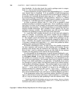
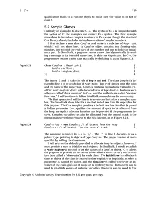
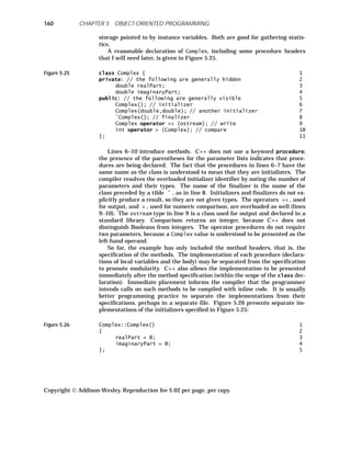
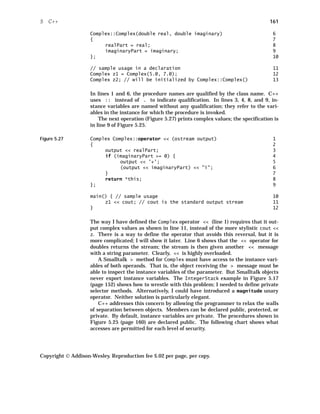
![Same Friend Subclass Client
Smalltalk instance variables n — y n
Smalltalk methods y — y y
C++ public members y y y y
C++ protected members y y y n
C++ private members y y n n
Each entry shows whether a member of an object O of class C is exported to
various contexts. “Same” means other objects of the same class C. C++ allows
such contexts access to instance variables; Smalltalk does not. Therefore, the
> operator in C++ has permission to access the instance variables of its pa-
rameter. “Friends” are procedures or classes that class C declares to be its
friends. Friends are permitted to refer to all members of instances of C. More
restrictively, a method M may declare procedures and classes to be its friends;
those friends are permitted to invoke M even though M may be hidden to oth-
ers. “Subclass” refers to code within subclasses of C. Subclasses have access
to all members except for private ones in C++. “Clients” are instances of
classes unrelated to C.
The design of C++ makes it easier to deal with binary operations that take
two instances of the same class than in Smalltalk. All instance variables of
one instance are visible to the other. For example, the implementation of
> (the specification is in line 10 of Figure 5.25 on page 160) can inspect the
instance variables of its formal parameter right (see Figure 5.28).
Figure 5.28 int Complex::operator > (Complex right) 1
{ 2
double leftmag, rightmag; 3
leftmag = (realPart * realPart) + 4
(imaginaryPart * imaginaryPart); 5
leftmag = (right.realPart * right.realPart) + 6
(right.imaginaryPart * right.imaginaryPart); 7
return leftmag > rightmag; 8
} 9
C++ lets subclasses further restrict the visibility of identifiers by explicitly re-
declaring all inherited public and protected identifiers protected or private.
(Subclasses do not inherit private identifiers.)
Other security arrangements are possible. In Oberon-2, instance vari-
ables may be exported read-write, exported readonly, or not exported at all
[Reiser 92]. Oberon-2 does not distinguish between exports to other classes
and inheritance by subclasses.
Polymorphism in C++ is achieved by generic classes. A generic Stack
class that can be instantiated (at compile time) to become a class of any given
type, including a stack of stacks, can be written as in Figure 5.29.
Copyright Addison-Wesley. Reproduction fee $.02 per page, per copy.
162 CHAPTER 5 OBJECT-ORIENTED PROGRAMMING](https://image.slidesharecdn.com/advancedprogramminglanguagedesign-230706034617-464d64c2/85/Advanced_programming_language_design-pdf-170-320.jpg)
![163
Figure 5.29 #define MAXSIZE 10 1
template <class BaseType> class Stack { 2
private: 3
BaseType elements[MAXSIZE]; 4
int count; 5
public: 6
Stack() { // initializer 7
count = 0; 8
} 9
void Push(BaseType element) { 10
elements[count] = element; 11
count = count + 1; 12
} 13
BaseType Pop() { 14
count = count - 1; 15
return(elements[count]); 16
} 17
int Empty() { 18
return(count == 0); 19
} 20
friend ostream 21
operator << (ostream output, Stack<BaseType> S) { 22
int index; 23
output << "["; 24
for (index = 0; index < S.count; index++) { 25
output << S.elements[index]; 26
if (index+1 == S.count) break; 27
output << ","; 28
} 29
output << "]"; 30
return(output); 31
} // << 32
}; // Stack 33
main(){ // sample usage 34
Stack<int> myIntStack; 35
Stack<float> myFloatStack; 36
Stack<Stack<int> > myRecursiveStack; 37
myIntStack.Push(4); 38
myIntStack.Push(8); 39
cout << myIntStack; // [4,8] 40
myFloatStack.Push(4.2); 41
cout << myFloatStack; // [4.2] 42
myRecursiveStack.Push(myIntStack); 43
cout << myRecursiveStack; // [[4,8]] 44
} 45
The definition in line 1 effectively declares MAXSIZE a constant with value 10.
The template declaration in line 2 indicates that Stack is parameterized by a
type (literally, by a class). I have ignored all error conditions in the methods
for simplicity’s sake. The declarations in lines 35–37 show how to supply pa-
rameters to the generic class; a generic class must have all parameters bound
in order to declare a variable. The compiler compiles a specific class sepa-
Copyright Addison-Wesley. Reproduction fee $.02 per page, per copy.
5 C++](https://image.slidesharecdn.com/advancedprogramminglanguagedesign-230706034617-464d64c2/85/Advanced_programming_language_design-pdf-171-320.jpg)
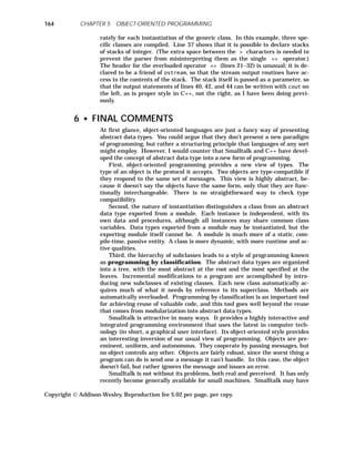
![165
been too quick to abandon concepts common in imperative programming lan-
guages. For example, it makes no provision for named constants; you must
create a variable and then be careful not to change it. This shortcoming could
easily be overcome without injustice to the design of the language. Similarly,
it would be nice to introduce some type checking (even if dynamically
checked) by allowing variables to have a type (that is, a class) specifier. Pro-
grams would be easier to read and less error-prone. It might also make ma-
nipulation of variables more efficient, particularly for primitive types. As a
small step in this direction, Smalltalk suggests that identifiers like anInte-
ger or aStack be used conventionally for variables whose class is meant to be
fixed. Of course, an identifier named anInteger need not actually map to an
integer under Smalltalk’s rules. Finally, Smalltalk provides no control over
whether identifiers are exported (instance variables aren’t, methods are) or
inherited (all are). A finer level of control, such as that provided by C++,
could improve the safety of programs.
C++ fixes some of these problems. First, types and methods are bound at
compile time. Numeric values and code blocks are not objects at all. There is
no need to understand expressions as evaluated by messages sent to objects.
The result is that C++ programs execute quite efficiently, because they usu-
ally avoid Smalltalk’s dynamic method binding, use ordinary procedure invo-
cation, and use inline code to accomplish arithmetic. Second, members can be
individually controlled with regard to export and inheritability. The concept
of friends allows identifiers to be exported only to instances of particular
classes.
However, C++ suffers from its ancestry; C is notorious for being error-
prone (the operators for equality and assignment are easily confused, for ex-
ample), syntactically obscure (complicated types are hard for humans to
parse), and unsafe (loopholes allow all type checking to be circumvented).
Other object-oriented languages have been designed, of course. Best
known perhaps is Eiffel [Meyer 92]. Nor is C the only language that has been
extended to give it an object orientation. Other good examples include CLOS
(the Common LISP Object System) and [incr Tcl]. Some people believe that
Ada 95 will be the most widespread object-oriented programming language in
a few years. Even object-oriented COBOL has been considered [Clement 92].
EXERCISES
Review Exercises
5.1 What are the consequences in C++ of static typing?
5.2 Does an object in Smalltalk require its own private stack? In C++?
5.3 Write a class in Smalltalk and/or in C for rational numbers, that is,
numbers that can be represented by an integer numerator and denomi-
nator. Instance variables should include both the numerator and the
denominator. Your implementation should always reduce fractions to
their lowest terms. You must overload all arithmetic and conditional op-
erators.
Copyright Addison-Wesley. Reproduction fee $.02 per page, per copy.
EXERCISES](https://image.slidesharecdn.com/advancedprogramminglanguagedesign-230706034617-464d64c2/85/Advanced_programming_language_design-pdf-173-320.jpg)
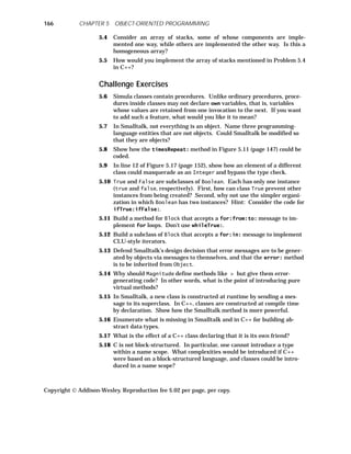


![h
hhhhhhhhhhhhhhhhhhhhhhhhhhhhhhhhhhhhhhhhhhhhhhhhhhhhhhhhhhhhhhhhhhhhhhhhhhhhhhhhhhhhhhhhhhh
Chapter 6 ❖
Dataflow
There is some evidence that the next big wave of change to wash over pro-
gramming languages will be concurrency. Both architectures and languages
for concurrency have been around for some time. In this chapter, I will dis-
cuss the dataflow architectural concept and the languages that have been de-
signed to conform to it. Dataflow is one way to achieve concurrency,
particularly at the fine-grain level: It finds multiple operations that can be
undertaken concurrently within the evaluation of a single expression. Ideas
from dataflow have found their way into parallelizing compilers for more con-
ventional architectures, as well. The ideas here in some ways prepare for
Chapter 7, which deals with concurrent programming languages that work at
a coarser level of granularity.
Sequential execution is an essential characteristic of the von Neumann
computer architecture, in which programs and data are stored in a central
memory. The concepts embodied by classical architecture have not been di-
rectly applicable to the domain of parallel computation. Most programming
languages have evolved from von Neumann languages, designed specifically
for the von Neumann architecture, so programmers have been conditioned to
analyze problems and write programs in sequential fashion.
The dataflow approach was first suggested by Karp and Miller [Karp 66]
as an alternative to the von Neumann architectural and linguistic concepts.
Consider computation of the series of statements in Figure 6.1.
Figure 6.1 A := B*C + D/F; 1
G := H**2 + A; 2
A data-dependency graph called a dataflow graph represents the order-
ing of evaluation imposed by data dependencies. It encodes the fact that an
expression can’t be evaluated before its operands are evaluated. The dataflow
graph for Figure 6.1 appears in Figure 6.2.
hhhhhhhhhhhhhhhhhhhhhhhhhhhhhhhhhhhh
On-line edition copyright 1996 by Addison-Wesley Publishing Company. Permission is
granted to print or photocopy this document for a fee of $0.02 per page, per copy, payable to Addi-
son-Wesley Publishing Company. All other rights reserved.
169](https://image.slidesharecdn.com/advancedprogramminglanguagedesign-230706034617-464d64c2/85/Advanced_programming_language_design-pdf-177-320.jpg)
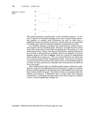
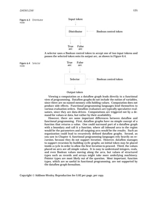
![1 ◆ DATAFLOW COMPUTERS
There are two classes of dataflow architectures. The first class is called
“static,” since such architectures do not support reentrant dataflow code (that
is, code that is used simultaneously in multiple places in the dataflow graph)
and recursion. The simple dataflow computer model introduced above is
static, as is the machine proposed by Dennis [Dennis 77].
The second class is called “dynamic.” Such machines support simultane-
ous multiple incarnations of an activity, recursion, and loop unfolding. In a
dynamic dataflow architecture, an arc may carry multiple tokens, and care is
taken to ensure that activities fire only upon receipt of matching tokens along
their input arcs. Tokens are labeled to distinguish values arising in different
contexts or from different incarnations of an activity. Two tokens match only
if their activity labels match. For example, I might wish to perform the com-
putation specified by a dataflow graph on each element of a vector of 1000
values. With a dynamic dataflow architecture, I can place 1000 tokens on the
input arc. Tokens are labeled to insure that values produced during the com-
putation can be ascribed to the appropriate input value.
The dynamic architecture outlined below is essentially that of the classical
Manchester Dataflow Computer [Gurd 85]. Modern dynamic dataflow archi-
tectures may look different. Tokens are labeled, but I leave out the specific
details of how the labels are generated or used, except that labels are
matched to identify matching tokens.
The architecture is schematically depicted in Figure 6.5. The machine op-
erates as a circular pipeline divided into four sections. The processing unit
receives packets containing operands and an instruction. The instruction is
executed on the accompanying operands, and the result tokens (after appro-
priate labeling) are placed back on the bus to be sent to the I/O switch. The
I/O Switch is included in the pipeline to serve as an I/O port. The matching
unit consists of associative token storage. When a token arrives at the
matching unit, the storage is searched for any tokens with the same label and
destination. If matches are discovered, these tokens are read out of the store,
and a packet is formed of all these tokens to be sent on to the program store.
The destination field of a token carries the address in the program store of
the instruction to which the token is directed.
Copyright Addison-Wesley. Reproduction fee $.02 per page, per copy.
172 CHAPTER 6 DATAFLOW](https://image.slidesharecdn.com/advancedprogramminglanguagedesign-230706034617-464d64c2/85/Advanced_programming_language_design-pdf-180-320.jpg)
![173
Figure 6.5 Dataflow
architecture
Matching unit
I/O switch
Program store
Processing unit
If no match for the arriving token is found in the matching store, the to-
ken is written into storage and held in abeyance for matching tokens ex-
pected to arrive in the future. For unary operators, no matching is needed,
and the token can bypass the matching unit and proceed directly to the pro-
gram store. It is estimated that 55–70 percent of all tokens are able to bypass
the matching section.
When a packet of tokens reaches the program store, the instruction to
which the tokens are directed is accessed, and a packet is formed of the to-
kens and the instruction. This instruction is an opcode, the operands being
already available in the packet. Opcodes are elementary operations like addi-
tion and multiplication. The program store effectively holds the dataflow
graph. Instructions are vertices, and the arcs are represented by link fields
associated with each instruction to indicate the successor nodes in the
dataflow graph. The packet consisting of the operands, the opcode, and suc-
cessor information is then sent to the processing unit, and the operation of
the machine continues as described.
2 ◆ VAL
Val is a dataflow language developed at MIT by J. Dennis and others
[McGraw 82]. This language was originally designed for the static dataflow
architecture of Dennis, so it does not support dynamic dataflow features like
recursion. Val has been meticulously defined both by an axiomatic
[Ackerman 80] and a denotational [Gehani 80] semantics (these concepts are
discussed in Chapter 10.) Val is functional in nature, so side effects are ab-
sent. However, Val is strongly typed (using structural equivalence) and in-
tentionally looks more like conventional languages than LISP or FP does. In
fact, it looks much like ML (described in Chapter 3). For example, the Val
function in Figure 6.6 computes the mean and standard deviation for parame-
ters X, Y, and Z.
Copyright Addison-Wesley. Reproduction fee $.02 per page, per copy.
2 VAL](https://image.slidesharecdn.com/advancedprogramminglanguagedesign-230706034617-464d64c2/85/Advanced_programming_language_design-pdf-181-320.jpg)
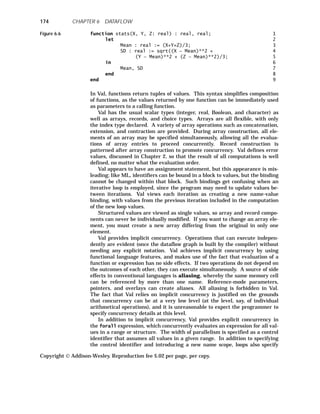
![175
how to merge the values from all the parallel streams into one result. There
are two ways to generate results: construct, which allows each parallel exe-
cution path to generate a value that becomes an element of an array of re-
sults, and accumulate, in which values from all the result streams are
merged into one result using one of a fixed set of associative binary operators
like + . (The operation specified by accumulate can be computed by an im-
plicit balanced binary tree, allowing the merged value to be produced in loga-
rithmic time.) Figure 6.7 clarifies these notions.
Figure 6.7 forall i in [1, 100] do 1
left: real := point[i].x_low; 2
bottom: real := point[i].y_low; 3
right: real := point[i].x_high; 4
top: real := point[i].y_high; 5
area: real := (right−left) * (top−bottom); 6
okay: Boolean := acceptable(area); 7
abort: Boolean := erroneous(area); 8
accumulate + if okay then area else 0.0 end; 9
accumulate or abort; 10
construct if okay then area else 0.0 end; 11
end 12
In this program, the forall produces 100 concurrent streams of execution.
Their results are merged using accumulate + to add all acceptable areas (line
9), accumulate or to determine if abort was true in any of the streams (line
10), and construct to create an array of elements calculated by a formula
(line 11). The entire forall expression returns a 3-tuple comprising those
three results.
The for expression implements loops that cannot execute in parallel be-
cause values produced in one iteration must be used in the next. The decision
concerning whether to continue loop iteration occurs within the loop body as a
conditional expression, as in Figure 6.8.
Copyright Addison-Wesley. Reproduction fee $.02 per page, per copy.
2 VAL](https://image.slidesharecdn.com/advancedprogramminglanguagedesign-230706034617-464d64c2/85/Advanced_programming_language_design-pdf-183-320.jpg)
![Figure 6.8 for 1
a: real := 0.0; 2
b: real := 1.0; 3
do 4
let 5
c: real, done: Boolean := Compute(a, b); 6
in 7
if done then 8
c 9
else 10
iter 11
a := NewA(a, b); 12
b := NewB(a, b); 13
end 14
end 15
end 16
end 17
The identifiers a and b (lines 2 and 3) are loop parameters. During the first
iteration of the loop, the parameters have values 0.0 and 1.0. The Compute
invocation (line 6) returns two values, which are bound to c and done. If iter
is selected (lines 11–14), a new iteration is begun. New values for a and b are
evaluated for the next iteration. The binding in line 13 uses the old value of a
on the right-hand side. When done is true, the expression returns the value
bound to c (line 9).
A choice type is built as shown in Figure 6.9.
Figure 6.9 type list = 1
choice [ 2
empty : void; 3
nonempty : record [item : real; rest : list] 4
] 5
Void (line 3) is a predeclared type with no values. This example defines list
as an ordinary linked list, but with an interesting difference — it is recur-
sively defined without using pointers. Val disallows pointers because of alias-
ing issues. A list is therefore a recursive data structure rather than a
sequence of individual elements linked with pointers.
A value of a choice type is created by using a make constructor (Figure
6.10).
Figure 6.10 make list[empty : nil]
To guarantee type compatibility, the contents of a choice can only be accessed
via tagcase, as in Figure 6.11.
Copyright Addison-Wesley. Reproduction fee $.02 per page, per copy.
176 CHAPTER 6 DATAFLOW](https://image.slidesharecdn.com/advancedprogramminglanguagedesign-230706034617-464d64c2/85/Advanced_programming_language_design-pdf-184-320.jpg)
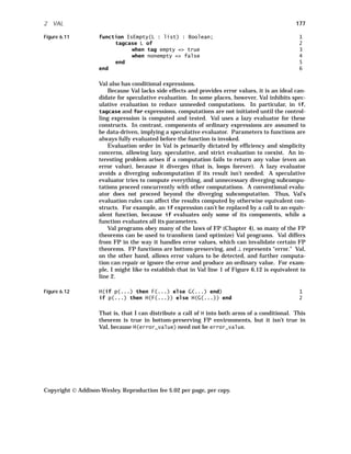
![3 ◆ SISAL
Val was one of the first serious attempts to produce a production-quality
dataflow language. A descendent of Val called Sisal was created to exploit the
capabilities of dynamic dataflow computers [McGraw 83]. A Sisal compiler
exists, with code generators for Vax, Crays, HEP multiprocessors, and the
Manchester dataflow computer.
The most obvious advantage of Sisal over Val is its support of recursion.
Recursive functions are useful and natural, especially in functional lan-
guages. Val’s rejection of recursion was a reflection of the design of early
static dataflow machines. Sisal also supports streams, which are needed for
ordinary sequential I/O and as a means of composing functions.
Sisal programs can be decomposed into distinct compilation units that ex-
plicitly import and export functions. Sisal also extends Val’s iterative and
parallel (forall) loop forms. They can return arrays or streams. Parallel
loops can also define explicit inner and outer products, making array manipu-
lation cleaner and potentially more efficient.
4 ◆ POST
Chinya V. Ravishankar developed Post as a Ph.D. thesis starting in 1981
[Ravishankar 89]. Post introduces several novel ideas. First, it lets the pro-
grammer determine the level of speculation in evaluation. As I mentioned
earlier, speculative evaluation can lead to nontermination under certain cir-
cumstances, but strictly lazy evaluation reduces parallelism. A second novel
concept is polychronous data structures that are partly synchronous
(must be available before used) and partly asynchronous (parts can be used
when ready). Third, Post provides communication between computational ac-
tivities in order to terminate speculative computation that may turn out to be
unnecessary. Communication between computations is not natural in purely
functional programming languages. Much of their semantic elegance derives
from their lack of side effects, so computations scheduled in parallel must not
depend on each other’s results. Further, a purely functional language per-
mits only deterministic computations and prohibits history-sensitivity.
Post was never fully implemented, but a prototype compiler was built. It
first builds a dataflow graph from the program and then converts that graph
into instructions for a dynamic dataflow machine. Post needs a dataflow ma-
chine (never implemented) that has a few special features, such as a “hold”
node for implementing lazy evaluation and a “terminate store” to help find
and remove terminated tokens.
4.1 Data Types
Values can be either primitive (integer, real, Boolean, char) or structured.
Structured values are constructed using the abstractions stream and tuple.
Both are sequences of values, but a tuple may be heterogeneous and is of
fixed length, while a stream is homogeneous and of unbounded length. All
operators and functions are automatically overloaded to apply to streams;
they create streams of results of pointwise application. Nested structures are
allowed; an element of a stream may itself be a stream.
Copyright Addison-Wesley. Reproduction fee $.02 per page, per copy.
178 CHAPTER 6 DATAFLOW](https://image.slidesharecdn.com/advancedprogramminglanguagedesign-230706034617-464d64c2/85/Advanced_programming_language_design-pdf-186-320.jpg)
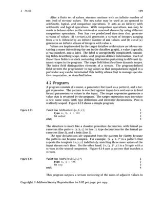
![the input stream; the order of the output stream matches the order of the in-
put stream. If the input stream consists of an odd number of elements, y in
the final instance of the template matches an eos token, which is an identity
for arithmetic operations.
4.3 Synchrony Control
By using connectors other than a comma, the programmer may specify the
degree of synchrony required in pattern matching. The comma indicates
completely asynchronous matching; the actual parameters may be accessed
independently of each other. If the pattern uses only ˆ , matching is syn-
chronous: all elements must be present before any element is made available
to the target expression.1
If the pattern uses only ˜ , matching is sequential:
the ith element of the matched data structure is available only after all previ-
ous elements have arrived (even if they have not been accessed). Any or all of
these combinators may occur within a pattern. If several of them occur, ac-
cess is polychronous; precedence rules indicate how to group subpatterns in
the absence of parentheses.
In Figure 6.14, I could change the input pattern to {xˆy,}*, forcing pair-
wise synchronization of input elements. The program would compute the
same results, because + requires both operands before proceeding.
Sequential patterns are used for loops, as shown in the Figure 6.15.
Figure 6.15 function Largest{x˜}* init 0; 1
type x : int 2
in if Largest > x then Largest else x end 3
end; 4
This program finds the largest value in a stream of integers. It terminates
when the last instance of the target expression terminates; the value gener-
ated in this last instance is returned as the value of the program. The pro-
gram name is used to name the current value, initialized to 0 in line 1 and
compared with the next value in line 3. The dataflow graph corresponding to
this program has a cycle holding an initial token with value 0. Conditional
expressions, like the one in line 3, are evaluated speculatively. The result
from the branch that is not needed is discarded after evaluation is complete.2
An alternative syntax for conditionals is shown in Figure 6.16.
Figure 6.16 function OddSquares{x,}*; 1
type x : int 2
in [(x mod 2) ≠ 0] x*x 3
end;
Line 3 evaluates to x*x only if the condition in square brackets is true, that
hhhhhhhhhhhhhhhhhhhhhhhhhhhhhhhhhhhh
1
The concept of synchronization in concurrent programming languages is related; it is dis-
cussed in Chapter 7.
2
If conditionals were evaluated lazily, the programmer could hoist both branches out of the
conditional to force them to be evaluated speculatively.
Copyright Addison-Wesley. Reproduction fee $.02 per page, per copy.
180 CHAPTER 6 DATAFLOW](https://image.slidesharecdn.com/advancedprogramminglanguagedesign-230706034617-464d64c2/85/Advanced_programming_language_design-pdf-188-320.jpg)
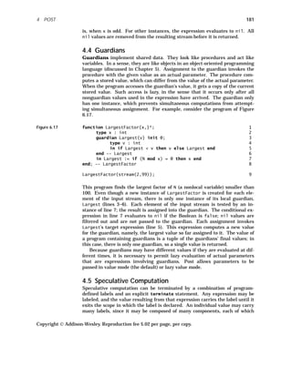
![may acquire multiple labels in different computations. Figure 6.18 is an ex-
ample of labeling.
Figure 6.18 function ReportEvens{x,}*; 1
type x : int; 2
label Even; 3
function AddLabel{y}; 4
type y : int 5
in 6
if (y mod 2) = 0 then 7
tag y with Even 8
else 9
y 10
end; 11
end; -- AddLabel 12
in [ AddLabel(x) haslabel Even ] x; 13
end; -- ReportEvens 14
This program returns only the even elements of the input stream. AddLabel
labels its parameter if the parameter is even (line 8). The body of Re-
portEvens in line 12 checks to see if its parameter, passed through AddLabel,
is labeled. If so, the parameter is returned; otherwise, the value nil is re-
turned (and then removed from the resulting stream).
If the program chooses to delete all tokens that have a particular label,
any computation they are involved in is thereby terminated. Figure 6.19
demonstrates termination.
Figure 6.19 function SomeFactor{x,}*; 1
type x : int; 2
guardian Factor{y}; 3
type y : int 4
in terminate y 5
end; -- Factor 6
in Factor := if (N mod x)=0 then x end; 7
end; -- SomeFactor 8
SomeFactor(stream(2,99)); 9
The program returns the first factor of N assigned to the guardian Factor; it
may return different values for different runs. For each input value, line 7
reports a factor, if any, to the guardian. The guardian Factor executes a ter-
minate statement and returns the value y (line 5). The terminate statement
does not specify a label in this case; all computation in the current scope
(which is implicitly given a scope label) is canceled. There is also a syntax
(not shown in this example) for specifying a program-defined label to control
termination.
Copyright Addison-Wesley. Reproduction fee $.02 per page, per copy.
182 CHAPTER 6 DATAFLOW](https://image.slidesharecdn.com/advancedprogramminglanguagedesign-230706034617-464d64c2/85/Advanced_programming_language_design-pdf-190-320.jpg)
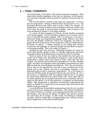
![EXERCISES
Review Exercises
6.1 Draw a dataflow graph for the code of Figure 6.20.
Figure 6.20 (A + B) * (A + B + C)
6.2 Draw a dataflow graph for the code of Figure 6.21.
Figure 6.21 A := 0; 1
while A < 10 do 2
A := A + 3; 3
end; 4
6.3 How do nondataflow languages allow the programmer to specify evalua-
tion strategy?
Challenge Exercises
6.4 Draw a dataflow graph for the code of Figure 6.22.
Figure 6.22 procedure Orbit(A : integer) : integer; 1
begin 2
if A = 1 then 3
return 1; 4
elsif even(A) then 5
return Orbit(A/2); 6
else 7
return Orbit(3*A+1); 8
end; 9
end; 10
6.5 In Figure 6.15 (page 180), which version of > is meant on line 3? That
is, does eos act as the minimal or maximal element?
6.6 In Figure 6.18 (page 182), what would be the effect of changing line 13
as follows?
in [ AddLabel(x) haslabel Even] AddLabel(x)
6.7 Modify Figure 6.19 (page 182) so that speculative computation is not
terminated, but the first factor found is still returned.
6.8 In spreadsheets, how can reevaluating more than once have a different
effect from evaluating only once?
Copyright Addison-Wesley. Reproduction fee $.02 per page, per copy.
184 CHAPTER 6 DATAFLOW](https://image.slidesharecdn.com/advancedprogramminglanguagedesign-230706034617-464d64c2/85/Advanced_programming_language_design-pdf-192-320.jpg)


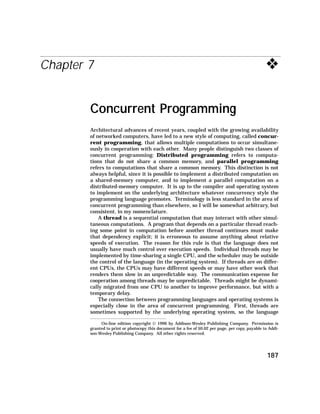
![implementation needs to make use of those facilities, and the language de-
signer may choose to present or to omit features, depending on the operating
system and what it can do. For example, a thread can be modeled by a Unix
process. Generally, Unix processes cannot share memory. However, some
versions of Unix, such as Solaris, offer threads within a single address space;
these threads do share memory. Second, operating systems themselves are
often multithreaded; the language design issues in this chapter are often
identical with operating-system design issues.
1 ◆ STARTING MULTIPLE THREADS
Syntax for starting multiple computations tends to be straightforward. In
Modula (I mean original Modula [Wirth 77], not Modula-2), a thread is
started by invoking a procedurelike object; when the “procedure” returns, the
thread disappears. Meanwhile, the computation that started the thread con-
tinues executing. The new thread may itself create other threads by invoking
them. Figure 7.1 shows a program that merge-sorts an array by recursively
creating threads.
Figure 7.1 type 1
DataArray = array whatever of integer; 2
thread MergeSort( 3
reference Tangled : DataArray; 4
value LowIndex, HighIndex : integer); 5
variable 6
MidPoint : integer := (LowIndex + HighIndex) div 2; 7
begin 8
if LowIndex + 1 < HighIndex then -- worth sorting 9
MergeSort(Tangled, LowIndex, MidPoint); 10
MergeSort(Tangled, MidPoint+1, HighIndex); 11
Merge(Tangled, 1, MidPoint, MidPoint+1, 12
HighIndex); 13
end; -- worth sorting 14
end; -- MergeSort 15
MergeSort is declared in line 3 as a thread, not a procedure. All invocations
of MergeSort, including the recursive ones on lines 10 and 11, create new
threads running instances of MergeSort that work independently of the main
program. Unfortunately, MergeSort fails to wait for its children to finish and
rushes ahead to line 12, merging the two halves of the array before they are
properly sorted. You will soon see mechanisms for synchronization that will
let me fix this bug.
Each thread gets its own stack. Variables declared locally to a thread are
like local variables in a procedure; each thread gets its own local variables.
Likewise, any procedures called from a thread (such as Merge, called in line
12) get new activation records on the thread’s stack. However, variables that
are outside the scope of the thread are shared among all threads in which
they are visible by normal scope rules. That is, the static chain in a thread’s
stack eventually points outside of the private stack of the thread into shared
stack. (Sometimes this arrangement is called a cactus stack, since the
Copyright Addison-Wesley. Reproduction fee $.02 per page, per copy.
188 CHAPTER 7 CONCURRENT PROGRAMMING](https://image.slidesharecdn.com/advancedprogramminglanguagedesign-230706034617-464d64c2/85/Advanced_programming_language_design-pdf-196-320.jpg)
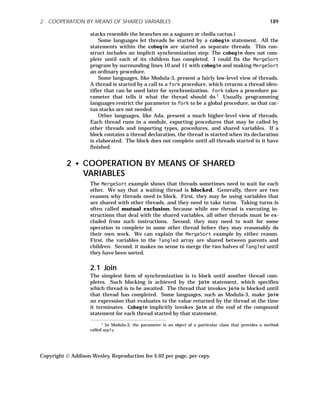
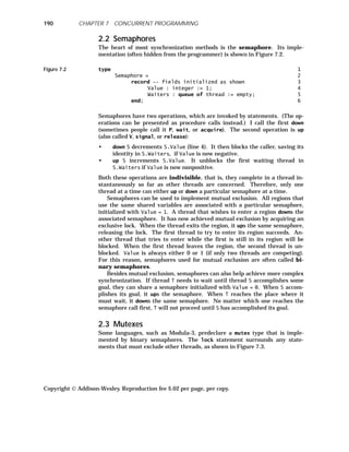
![191
Figure 7.3 variable 1
A, B : integer; 2
AMutex, BMutex : mutex; 3
procedure Modify(); 4
begin 5
lock AMutex do 6
A := A + 1; 7
end; 8
lock BMutex do 9
B := B + 1; 10
end; 11
lock AMutex, BMutex do 12
A := A + B; 13
B := A; 14
end; 15
end; -- Modify 16
Variable A is protected by mutex AMutex, and B is protected by BMutex. The
lock statement (as in line 6) is equivalent to a down operation at the start and
an up operation at the end. Several threads may simultaneously execute in
Modify. However, a thread executing line 7 prevents any other thread from
executing any of lines 7, 13, and 14. It is possible for one thread to be at line
7 and another at line 10. I lock lines 7 and 10 because on many machines, in-
crementing requires several instructions, and if two threads execute those in-
structions at about the same time, the variable might get incremented only
once instead of twice. I lock lines 13 and 14 together to make sure that no
thread can intervene after line 13 and before line 14 to modify A. The multi-
ple lock in line 12 first locks AMutex, then BMutex. The order is important to
prevent deadlocks, as I will describe later.
2.4 Conditional Critical Regions
The Edison language has a way to program synchronization that is more ex-
pressive than mutexes but less error-prone than bare semaphores
[Brinch Hansen 80]. As I mentioned before, synchronization in general is the
desire to block an action until a particular condition becomes true.
A standard example that displays the need for synchronization is the
bounded buffer, which is an array that is filled by producer threads and
emptied by consumer threads. All producers and consumers must mutually
exclude each other while they are inspecting and modifying the variables that
make up the bounded buffer. In addition, when the buffer is full, producers
should block instead of busy waiting, which is repeatedly testing to see if
the buffer has room. Likewise, when the buffer is empty, consumers should
block. Figure 7.4 shows how to code this application with conditional critical
regions.
Copyright Addison-Wesley. Reproduction fee $.02 per page, per copy.
2 COOPERATION BY MEANS OF SHARED VARIABLES](https://image.slidesharecdn.com/advancedprogramminglanguagedesign-230706034617-464d64c2/85/Advanced_programming_language_design-pdf-199-320.jpg)
![Figure 7.4 constant 1
Size = 10; -- capacity of the buffer 2
type 3
Datum = ... -- contents of the buffer 4
variable 5
Buffer : array 0..Size-1 of Datum; 6
InCount, OutCount : integer := 0; 7
procedure PutBuffer(value What : Datum); 8
begin 9
region Buffer, InCount, OutCount 10
await InCount - OutCount < Size do 11
Buffer[InCount mod Size] := What; 12
InCount := InCount + 1; 13
end; -- region 14
end -- PutBuffer; 15
procedure GetBuffer(result Answer : Datum); 16
begin 17
region Buffer, InCount, OutCount 18
await InCount - OutCount > 0 do 19
Answer := Buffer[OutCount mod Size]; 20
OutCount := OutCount + 1; 21
end; -- region 22
end GetBuffer; 23
The region statements starting in lines 10 and 18 are like lock statements,
except that they name variables to be protected, not mutexes, and they have
an await component. The compiler can check that shared variables are only
accessed within region statements, and it can invent appropriate mutexes.
The awaited condition is checked while the corresponding mutexes are held.
If the condition is false, the mutexes are released and the thread is blocked
(on an implicit semaphore). Whenever a thread exits from a region, all
threads in conflicting regions (those that use some of the same shared vari-
ables) that are blocked for conditions are unblocked, regain their mutexes,
and test their conditions again. This repeated rechecking of conditions can be
a major performance problem.
2.5 Monitors
One objection to using conditional critical regions is the cost of checking con-
ditions, which must occur whenever a thread leaves a region. A second objec-
tion is that code that modifies shared data may be scattered throughout a
program. The monitor construct, found in Modula and Mesa, was invented to
address both issues [Hoare 74; Lampson 80]. It acts both as a data-
abstraction device (providing modularity) and a synchronization device.
Monitors introduce a new name scope that contains shared data and the
procedures that are allowed to access the data. Procedures exported from the
monitor are mutually exclusive; that is, only one thread may execute an ex-
ported procedure from a particular monitor at a time.
The most straightforward use of monitors is to package all routines that
use a set of shared data (represented by a collection of variables) into a single
Copyright Addison-Wesley. Reproduction fee $.02 per page, per copy.
192 CHAPTER 7 CONCURRENT PROGRAMMING](https://image.slidesharecdn.com/advancedprogramminglanguagedesign-230706034617-464d64c2/85/Advanced_programming_language_design-pdf-200-320.jpg)
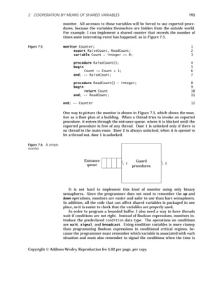
![right. A bounded buffer can be programmed as in Figure 7.7.
Figure 7.7 monitor BoundedBuffer; 1
export GetBuffer, PutBuffer; 2
constant 3
Size = 10; -- capacity of the buffer 4
type 5
Datum = ... -- contents of the buffer 6
variable 7
Buffer : array 0:Size-1 of Datum; 8
InCount, OutCount : integer := 0; 9
NotEmpty, NotFull : condition; 10
procedure PutBuffer(value What : Datum); 11
begin 12
if InCount - OutCount = Size then 13
wait NotFull; 14
end; 15
Buffer[InCount mod Size] := What; 16
InCount := InCount + 1; 17
signal NotEmpty ; 18
end; -- PutBuffer; 19
procedure GetBuffer(result Answer : Datum); 20
begin 21
if InCount - OutCount = 0 then 22
wait NotEmpty; 23
end; 24
Answer := Buffer[OutCount mod Size]; 25
OutCount := OutCount + 1; 26
signal NotFull ; 27
end; -- GetBuffer; 28
end; -- BoundedBuffer; 29
The situations in which the buffer is not full or not empty are indicated by
the condition variables NotFull and NotEmpty. Consumers call GetBuffer
(line 20), which checks to see if the buffer is empty. If so, it waits on NotEmpty
(line 23). This operation releases mutual exclusion and blocks the thread. It
will remain blocked until some other thread signals NotEmpty. Producers do
exactly that in line 18. Signal has no effect on a condition for which no
thread is waiting, unlike up on a semaphore. The consumer can be sure when
it arrives at line 25 that the buffer is not empty, because either it was not
empty when the consumer called GetBuffer, and this routine excludes any
other threads from the monitor, or it was empty, but some producer has sig-
naled NotEmpty, and the consumer has been awakened and regained exclu-
sion.
This discussion raises some troubling questions. Exactly when does the
blocked consumer continue? If immediately, then there may be two threads
in the monitor at once, and mutual exclusion is ruined. If later, then by the
time the consumer continues, some other consumer may already have taken
Copyright Addison-Wesley. Reproduction fee $.02 per page, per copy.
194 CHAPTER 7 CONCURRENT PROGRAMMING](https://image.slidesharecdn.com/advancedprogramminglanguagedesign-230706034617-464d64c2/85/Advanced_programming_language_design-pdf-202-320.jpg)
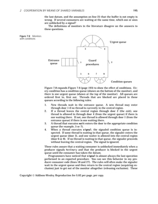
![extra waits ands locks are inefficient. If signal is not the last operation, the
signaler can’t assume that the situation of shared variables is unchanged
across signal. While it was in the urgent queue, the thread that was un-
blocked is likely to have modified the variables. The result is that signal is
error-prone. For these reasons, some languages require that signal must be
the last operation of an exported procedure and must cause the signaling
thread to leave the monitor. Then the implementation doesn’t need an urgent
queue, and signalers never make invalid assumptions about shared data.
However, this restriction makes monitors less expressive. (Such monitors are
strictly less powerful in a theoretical sense.)
A related suggestion is to use broadcast instead of signal. Broadcast re-
leases all the members of the given condition queue. Since they can’t all be
allowed into the central region at once, most are placed in the urgent queue.
A released thread can no longer assume that the condition it has awaited is
still met by the time it resumes. Programs written with broadcast usually
replace the if statement in lines 13 and 22 of Figure 7.7 with a while loop to
retest the condition after wait returns.
Proper use of monitors follows the guideline that no thread should take
too long in the central region. It shouldn’t take too long for a thread that is
waiting in the entrance queue to get into the monitor and access the shared
variables. Any lengthy operation should relax exclusion by entering a condi-
tion queue or by doing its work outside the monitor. A fascinating violation of
this guideline arises if the thread in an exported procedure makes a call on a
procedure exported by another monitor. Under the rules, this thread is still
considered to be in the first monitor, preventing any other thread from enter-
ing. However, it may take a long time before it returns because it may be
forced to wait in the second monitor in a condition queue. (By the guideline,
it shouldn’t have to wait very long in either the entrance queue or the urgent
queue.) This delay in returning violates the guideline with respect to the first
monitor. The situation can even lead to deadlock if the condition it awaits in
the second monitor can be signaled only by a thread that is currently waiting
patiently to enter the first monitor.
Several solutions have been proposed to this nested-monitor problem
[Haddon 77]:
1. Disallow nested monitor calls.
2. Warn the programmer, but allow the bad situation to develop. That is,
nested monitor calls maintain exclusion on the old monitor while in the
new one.
3. Release exclusion on the old monitor and enforce it only on the new one.
When the thread is ready to return, it must wait in the urgent queue of
the first monitor until it can once again achieve exclusive use of the cen-
tral region.
4. Let the programmer decide whether the nested call should maintain ex-
clusion in the old monitor or not. By default, method 2 is used. The
programmer can say duckout to release exclusion while still in the mon-
itor and duckin to achieve exclusion again. These calls can bracket a
nested call to simulate method 3.
Although monitors represent an important advance over raw semaphores,
they do have significant problems. Monitors have been criticized for not pro-
Copyright Addison-Wesley. Reproduction fee $.02 per page, per copy.
196 CHAPTER 7 CONCURRENT PROGRAMMING](https://image.slidesharecdn.com/advancedprogramminglanguagedesign-230706034617-464d64c2/85/Advanced_programming_language_design-pdf-204-320.jpg)
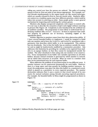
![monitor BoundedBuffer; 12
locks BufferPtrˆ using BufferPtr : BufferPtrType; 13
export GetBuffer, PutBuffer; 14
procedure PutBuffer( 15
value What : Datum; 16
value BufferPtr : BufferPtrType); 17
begin 18
if BufferPtrˆ.InCount-BufferPtrˆ.OutCount = Size 19
then 20
wait BufferPtrˆ.NotFull; 21
end; 22
BufferPtrˆ.Buffer[BufferPtrˆ.InCount mod Size] 23
:= What; 24
BufferPtrˆ.InCount := BufferPtrˆ.InCount + 1; 25
signal BufferPtrˆ.NotEmpty ; 26
end; -- PutBuffer; 27
procedure GetBuffer 28
(result Answer : Datum; 29
value BufferPtr : BufferPtrType); 30
begin 31
if BufferPtrˆ.InCount - BufferPtrˆ.OutCount = 0 32
then 33
wait BufferPtrˆ.NotEmpty; 34
end; 35
Answer := BufferPtrˆ.Buffer 36
[BufferPtrˆ.OutCount mod Size]; 37
BufferPtrˆ.OutCount := BufferPtrˆ.OutCount + 1; 38
signal BufferPtrˆ.NotFull ; 39
end; -- GetBuffer; 40
end; -- BoundedBuffer; 41
The buffer type (lines 5–10) implicitly contains a mutex. BoundedBuffer is
written as a monitor, which means it implicitly acquires and releases that
mutex on entrance and exit from exported procedures and when waiting for
conditions. The monitor specifies that it locks BufferPtrˆ, which must be a
parameter to every exported procedure. Unfortunately, if an exported proce-
dure modifies its parameter BufferPtr, chaos can ensue, since the wrong mu-
tex will then be accessed.
Modula-3 goes farther in solving the problem of overconservatism in moni-
tors. It gives up on monitors entirely, providing only the building blocks out
of which the programmer can build the necessary structures. That is, Mod-
ula-3 has conditions and mutexes as ordinary data types. The wait state-
ment specifies both a condition and a mutex. As the thread begins to wait, it
releases the mutex. When the thread is awakened by either signal or broad-
cast, it regains the mutex. Exported procedures and condition variables may
be packaged into modules (to make monitors), data structures (so that each
bounded buffer is independently exclusive), or classes (to allow monitors to be
instantiated any number of times).
A serious objection to monitors is related to the guideline that exclusion
should not be in force for very long. The problem is that shared data might be
needed for a very long time. This is exactly the situation in the readers-
Copyright Addison-Wesley. Reproduction fee $.02 per page, per copy.
198 CHAPTER 7 CONCURRENT PROGRAMMING](https://image.slidesharecdn.com/advancedprogramminglanguagedesign-230706034617-464d64c2/85/Advanced_programming_language_design-pdf-206-320.jpg)
![199
writers problem, in which some threads (the readers) need to read shared
data, and others (the writers) need to write those data. Writers must exclude
readers and all other writers. Readers must exclude only writers. Reading
and writing are time-consuming operations, but they always finish eventu-
ally. If we export Read and Write from the monitor, two readers cannot exe-
cute at the same time, which is too restrictive. Therefore, Read must not be a
monitor procedure; it must be external to the monitor. Proper use of Read
would call the exported procedures StartRead and EndRead around calls to
Read, but there is no assurance that a programmer will follow these rules.
Monitors can therefore fail to protect shared data adequately.
2.6 Crowd Monitors
Crowd monitors are a nice extension to monitors that address this last prob-
lem [Horn 77]. Crowd monitors distinguish exclusive procedures from ordi-
nary procedures within the monitor. Only exclusive procedures are mutually
exclusive. Ordinary procedures may be invoked only by activities that have
permission to do so; this permission is dynamically granted and revoked by
exclusive procedures. A skeleton of the crowd-monitor solution to the read-
ers-writers problem appears in Figure 7.10.
Figure 7.10 crowd monitor ReadWrite; 1
export StartRead, EndRead, Read, StartWrite, 2
EndWrite, Write; 3
variable 4
Readers : crowd Read; 5
Writers : crowd Read, Write; 6
exclusive procedure StartRead(); 7
... -- block the caller until reading is safe 8
enter Readers; 9
... 10
exclusive procedure EndRead(); 11
... 12
leave Readers; 13
... -- bookkeeping, maybe signal a waiting writer 14
exclusive procedure StartWrite(); 15
... -- block the caller until writing is safe 16
enter Writers; 17
... 18
exclusive procedure EndWrite(); 19
... 20
leave Writers; 21
... -- bookkeeping, maybe signal waiter 22
procedure Read(...); 23
... -- actually read from the shared data 24
Copyright Addison-Wesley. Reproduction fee $.02 per page, per copy.
2 COOPERATION BY MEANS OF SHARED VARIABLES](https://image.slidesharecdn.com/advancedprogramminglanguagedesign-230706034617-464d64c2/85/Advanced_programming_language_design-pdf-207-320.jpg)
![procedure Write(...); 25
... -- actually modify the shared data 26
end; -- ReadWrite 27
In lines 5 and 6, I declare two crowds called Readers and Writers. Threads
can dynamically enter and leave these crowds. Any member of Readers may
access the Read procedure (lines 23–24), and any member of Writers may ac-
cess both the Read and the Write procedure (lines 25–26). Threads initially
belong to no crowds. The exclusive procedures decide when it is appropriate
for a thread to enter or leave a crowd. They may use conditions to wait for
the right situation. When the exclusive procedure decides to let a reader pro-
ceed, it executes enter for the Readers crowd (line 9). Similarly, a guard can
let a writer enter the Writers crowd (line 17). Although any thread may call
Read and Write, because they are exported from the monitor, a runtime check
prevents threads from calling them if the threads are not in appropriate
crowds. A member only of Readers may not call Write, but, a member of
Writers may call either Read or Write, since both are specified in the defini-
tion of Writers (line 6).
2.7 Event Counts and Sequencers
Mutual exclusion is not always desirable because it limits concurrency. It is
also unnecessary in some cases on physically distributed computers. In fact,
if one hasn’t yet implemented mutual exclusion, the method discussed here
can be used to build semaphores to provide mutual exclusion, too [Reed 79].
Those semaphores will even allow simultaneous down operations on several
semaphores.
The first type needed is the event count. An event count is implemented
as a nondecreasing integer variable. It keeps a count of the number of events
of interest to the program, such as the number of times a variable has been
modified. Event counts have three operations:
1. advance E is used to signal the occurrence of events associated with
event count E. It has the effect of incrementing E indivisibly.
2. read E is an expression that evaluates to the value of the event count E.
If read returns some number n, then at least n advance operations must
have happened. By the time this number is evaluated, the event count
may have been advanced again a number of times.
3. await E reaches v waits for the event count E to have the value v. It
blocks the calling thread until at least v advance operations have oc-
curred. It is acceptable if more than v advance operations have occurred
when the thread is finally unblocked. This overshoot could result from
very frequent advance operations.
These definitions allow both await and read to be concurrent with advance,
since the programmer won’t care if read gives a somewhat stale value or if
await waits a trifle too long.
Figure 7.11 shows how to encode the bounded buffer using event counts.
For the time being, I assume that there is only one producer and one con-
sumer.
Copyright Addison-Wesley. Reproduction fee $.02 per page, per copy.
200 CHAPTER 7 CONCURRENT PROGRAMMING](https://image.slidesharecdn.com/advancedprogramminglanguagedesign-230706034617-464d64c2/85/Advanced_programming_language_design-pdf-208-320.jpg)
![201
Figure 7.11 -- other declarations as before 1
variable InEvents, OutEvents : eventcount := 0; 2
procedure PutBuffer(value What : Datum); 3
begin 4
await OutEvents reaches InCount − Size; 5
Buffer[InCount mod Size] := What; 6
advance InEvents; 7
InCount := InCount + 1; 8
end ; -- PutBuffer; 9
procedure GetBuffer(result Answer : Datum); 10
begin 11
await InEvents reaches OutCount; 12
Answer := Buffer[OutCount mod Size]; 13
advance OutEvents; 14
OutCount := OutCount + 1; 15
end; -- GetBuffer; 16
There is no need to worry that the consumer and producer will simultane-
ously access the same cell in Buffer. The producer will wait until the con-
sumer has taken the value from any cell before await in line 5 will allow it to
proceed to refill it. Similarly, the consumer knows that when it accesses a cell
of Buffer, the producer must have placed data there, or the await in line 12
would not have unblocked. Even if both advance operations (lines 7 and 14)
happen at the same time, there is no problem, because they deal with differ-
ent event counts. The bounded buffer may be used simultaneously by both
threads because it guarantees that the very same datum will never be
touched by both at once. I could have omitted InCount and OutCount, replac-
ing them with read InEvents and read OutEvents, respectively, but since
they are used for indices into Buffer, and read can return a stale value, I
used separate variables to make sure the right index was always computed.
The second data type for synchronization is the sequencer, which assigns
an arbitrary order to unordered events. A sequencer is implemented as a
nondecreasing integer variable, and has only one operation: ticket.
• ticket S is an expression that first evaluates to the current value of the
sequencer S and then increments S. This operation is indivisible.
Now I can implement a bounded buffer in which there are many produc-
ers. For simplicity, I will still have only one consumer. As before, consump-
tion and production need not exclude each other. Multiple producers will
take turns to make sure that they don’t write into the same cell in Buffer.
The new producer program is given in Figure 7.12.
Copyright Addison-Wesley. Reproduction fee $.02 per page, per copy.
2 COOPERATION BY MEANS OF SHARED VARIABLES](https://image.slidesharecdn.com/advancedprogramminglanguagedesign-230706034617-464d64c2/85/Advanced_programming_language_design-pdf-209-320.jpg)
![Figure 7.12 variable ProducerTurn : sequencer := 0; 1
procedure PutBuffer(value What : Datum); 2
variable SequenceNumber : integer; 3
begin 4
SequenceNumber := ticket ProducerTurn; 5
await InEvents reaches SequenceNumber; 6
-- wait for turn 7
await OutEvents reaches SequenceNumber − Size; 8
-- wait for Buffer 9
Buffer[SequenceNumber mod Size] := What; 10
advance InEvents; 11
end ; -- PutBuffer; 12
Each producer must await its turn to produce. The ticket operator in line 5
orders active producers. There will be no wait in line 6 unless another pro-
ducer has just grabbed an earlier ticket and has not yet arrived at line 11.
The await in line 8 makes sure that the cell in Buffer that is about to be
overwritten has been consumed. The advance in line 11 tells waiting con-
sumers that this cell in Buffer may be consumed, and it tells waiting produc-
ers that this thread has finished its turn.
The await in line 6 might seem unnecessary. It’s there to make sure that
producers write cells of Buffer in order, so that consumers may assume that
when InCount is advanced in line 11, the next cell of Buffer has new data.
Unfortunately, one effect of this imposed sequential behavior on producers is
that separate cells of Buffer cannot be written simultaneously. If the cells
are large, producers may exclude each other for a long time.
2.8 Barriers
Some computations occur in phases, and threads that finish one phase must
wait until all have finished until any may proceed to the next phase. The
barrier type provides the necessary synchronization. It has one operation:
• meet B causes the thread to block on barrier B until all threads have exe-
cuted a meet statement on B.
An example of barrier synchronization is a bottom-up version of MergeSort,
shown in Figure 7.13.
Figure 7.13 constant UpperBound = ... -- size of array 1
type DataArray = array 0..UpperBound of integer; 2
variable 3
Tangled : DataArray; 4
MergeBarrier : barrier UpperBound div 2; 5
Copyright Addison-Wesley. Reproduction fee $.02 per page, per copy.
202 CHAPTER 7 CONCURRENT PROGRAMMING](https://image.slidesharecdn.com/advancedprogramminglanguagedesign-230706034617-464d64c2/85/Advanced_programming_language_design-pdf-210-320.jpg)
![203
thread MergeSort(Start : integer); 6
variable Width : integer; 7
begin 8
Width := 1; 9
while Width < UpperBound+1 do -- a phase 10
-- Sort Tangled[Start .. Start+2*Width-1] 11
if Start mod Width = 0 -- participate 12
Merge(Tangled, Start, Start+Width-1, 13
Start+Width, Start+2*Width-1); 14
end; 15
meet MergeBarrier; -- ends phase 16
Width := 2 * Width; -- preparation for next phase 17
end; 18
end; -- MergeSort 19
begin -- main 20
for Start := 0 to UpperBound step 2 do 21
MergeSort(Start); -- creates a thread 22
end; 23
end; -- main 24
If UpperBound (line 1) is, say, 9, then line 22 starts five threads, each working
on a different two-element section of Tangled. Each thread enters the first
phase, sorting its own two-element section. Lines 13 and 14 sort that section,
assuming that the two subsections are already sorted. Each thread waits for
the phase to complete (line 16) before starting the next. MergeBarrier is de-
clared in line 5 with a capacity equal to the number of threads. Threads that
meet at the barrier wait until the full capacity of the barrier is reached. Only
half the threads active in one phase need to participate in the next phase;
they select themselves in line 12. Those that become inactive still participate
in the barrier in future phases in order to permit the active ones to make
progress.
Two-thread barriers can be implemented by shared variables and busy
waiting or by two semaphores. Multithread barriers can be built by various
combinations of two-thread barriers; there are also other ways to build them.
In most implementations, when the barrier is first initialized, it needs to
know exactly which threads will participate.
Some researchers have suggested that meet be split into two operations
[Gupta 89]. The first, arrive, indicates that the thread has finished the pre-
vious phase. The second, depart, indicates that the thread is about to start
the next phase. Between arrive and depart, the thread need not block if it
has useful work to do. Threads are blocked at depart until all threads have
arrived. This suggestion can increase the effective parallelism of a program
if there is significant work that can be done between phases. In the Merge-
Sort example, I could place arrive at line 16 and depart after line 17. Sepa-
rating arrive from depart, however, can lead to programming errors in
which the operations fail to balance. I am tempted to place depart after line
11, but then threads would depart before arriveing.
Copyright Addison-Wesley. Reproduction fee $.02 per page, per copy.
2 COOPERATION BY MEANS OF SHARED VARIABLES](https://image.slidesharecdn.com/advancedprogramminglanguagedesign-230706034617-464d64c2/85/Advanced_programming_language_design-pdf-211-320.jpg)
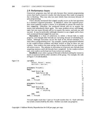
![205
The standard and simplest way to avoid deadlock is always to acquire re-
sources in the same order. If ThreadB would first lock Mutex1 and then Mu-
tex2, then there is no schedule that will lead to deadlock between these
threads. For this reason, languages that provide conditional critical regions
implicitly sort the necessary mutexes and acquire them in a standard order.
Of course, nested conditional critical regions can still deadlock.
Another way to deal with deadlock is to provide a way for wait statements
to be interrupted. Modula-3 provides a version of wait that will unblock if an
exception is raised in the thread. This exception can be raised by another
thread by the alert statement. The alert statement also sets a flag in the
alerted thread that it can inspect in case it is busy with a long computation
and is not waiting on a condition.
3 ◆ TRANSACTIONS: ARGUS
The concept of acquiring exclusion over data structures is often extended to
deal gracefully with failure. This behavior is especially important for pro-
grams that modify large shared databases. A transaction is a set of opera-
tions undertaken by a thread. Transactions have two important properties.
First, these operations are indivisible when taken as a whole. From the point
of view of other threads, either they have not started or they have all fin-
ished. Second, the transaction is recoverable; that is, it can either commit,
in which case all modifications to shared data take effect, or it can abort, in
which case none of its modifications takes effect. Because transactions are
indivisible, threads cannot see modifications performed by other transactions
that are still in progress.
For example, in an airline reservation database, a customer may wish to
exchange a seat on a given flight for a seat on another flight. The program
might give up the first seat and then reserve the second. If the second plane
is full, it is necessary to get back the initial seat, which may already have
been allocated to another passenger. If both actions (releasing the first seat
and reserving the second) are part of a transaction, then the program can just
abort when it fails to reserve the second seat. The first seat will still be re-
served by the original customer.
Transactions can be nested. In order to increase concurrency, programs
might want to start several threads as children of an initial thread. Each can
enter its own subtransaction. If any child thread fails, its own data modifica-
tions are recovered, but the parent transaction can still proceed. Unrelated
transactions do not see any data modifications until and unless the top-level
transaction commits.
Argus provides programming-language support for nested transactions
[Liskov 83a]. The statements comprising a transaction are the body of a
transaction statement. Of course, a procedure may be called from inside a
transaction, and the procedure may be recursive, so the lexical nature of
transaction entry does not limit the number of transactions. If the transac-
tion statements finish execution, the transaction commits. The statement
abort causes the current transaction to fail.
Data that are shared among threads must be built out of recoverable
types. Argus provides recoverable versions of primitive types, such as inte-
gers and arrays. Read and write locks are implicitly acquired when recover-
Copyright Addison-Wesley. Reproduction fee $.02 per page, per copy.
3 TRANSACTIONS: ARGUS](https://image.slidesharecdn.com/advancedprogramminglanguagedesign-230706034617-464d64c2/85/Advanced_programming_language_design-pdf-213-320.jpg)
![able variables are accessed. (These locks are typically held until the
transaction completes.) If a lock cannot be granted immediately because of
conflicting locks held by other threads, the accessing thread is blocked. Dead-
lock is automatically detected and handled by aborting one or more transac-
tions. It is also possible for a program to explicitly acquire a read or write
lock and to avoid blocking if the lock is not currently grantable. Structured
types can be made recoverable by providing access procedures that use mu-
tual exclusion and ensure that exclusion is only released when the structure’s
value is internally consistent.
These facilities can be used to build, for example, a bounded buffer of inte-
gers for which GetBuffer does not necessarily get the oldest remaining data
[Weihl 90], as in Figure 7.15.
Figure 7.15 module BoundedBuffer; 1
export GetBuffer, PutBuffer; 2
type 3
Entry = recoverable -- choice type 4
Valid : integer; 5
Invalid : void; 6
end; 7
variable 8
Buffer : array of Entry -- flexible; 9
procedure PutBuffer(value What : integer); 10
begin 11
region Buffer do -- get exclusion 12
Append(Buffer, 13
MakeRecoverable(Entry, Valid, What)); 14
end; 15
end; -- PutBuffer; 16
procedure GetBuffer(result Answer : integer); 17
variable Item : Entry; 18
begin 19
region Buffer do -- get exclusion 20
loop -- iterate until success 21
for Item in Buffer do 22
tagcase Item of 23
when writeable Valid(Answer) 24
=> ChangeRecoverable 25
(Item, Invalid); 26
return; 27
-- releases exclusion 28
end; -- writeable 29
end; -- tagcase 30
end; -- for Item 31
Copyright Addison-Wesley. Reproduction fee $.02 per page, per copy.
206 CHAPTER 7 CONCURRENT PROGRAMMING](https://image.slidesharecdn.com/advancedprogramminglanguagedesign-230706034617-464d64c2/85/Advanced_programming_language_design-pdf-214-320.jpg)
![207
duckout; -- release exclusion 32
sleep(); 33
duckin; -- regain exclusion 34
end; -- iterate until success 35
end; -- mutual exclusion 36
end; -- GetBuffer; 37
end; -- BoundedBuffer; 38
Enqueued integers are kept in the flexible array Buffer (line 9). Both Put-
Buffer and GetBuffer acquire mutual exclusion over the array by using re-
gion statements. Each item in the array is a recoverable object, which is a
choice type (lines 4–7). PutBuffer (lines 10–16) puts a new recoverable entry
in Buffer with the appropriate initial value. I use Append to add to the end of
a flexible array and MakeRecoverable to generate a new recoverable item
with an initial value. GetBuffer searches the array for an item on which it
can acquire a write lock and which is valid. I use a for loop (lines 22−31) to
scan through the flexible array. The tagcase statement (lines 23–30) checks
both the variant (I am interested only in Valid items) and whether a write
lock can be achieved. For those items where the variant is wrong or a write
lock cannot be achieved, the single branch of tagcase is not selected. For the
first item where the variant is correct and the write lock can be achieved,
GetBuffer stores the value in Answer (line 24), changes the value to Invalid
(Lines 25–26), and returns, releasing exclusion. If it fails to find such an
item, it releases exclusion, waits a while, then tries again (lines 32–34). Any
value returned by GetBuffer is guaranteed to have been placed there by a
transaction that is visible to the current one (that is, one that has committed
or is an ancestor of the current one) and not to have been removed by any ac-
tive or committed transaction. Invalid initial elements of the buffer can be
removed by a separate thread that repeatedly enters a top-level transaction
and removes elements that are writeable and invalid.
This example shows a few drawbacks to the way Argus deals with recover-
able types. Given the Argus facilities, it appears that the algorithm shown is
the most efficient that can be achieved. However, GetQueue is inefficient, be-
cause it needs to glance at all initial buffer entries, even if they are in use by
other transactions. It uses busy waiting in case it cannot find anything at the
moment. Programmers have no control over when commit and abort actually
make their changes, so it is possible for a consumer to get several items pro-
duced by the same producer out of order. Attempts to enhance the language
by adding transaction identifiers and explicit finalization code to be executed
upon commit or abort can relieve these shortcomings, but at the expense of
far more complicated programs [Weihl 90].
Copyright Addison-Wesley. Reproduction fee $.02 per page, per copy.
3 TRANSACTIONS: ARGUS](https://image.slidesharecdn.com/advancedprogramminglanguagedesign-230706034617-464d64c2/85/Advanced_programming_language_design-pdf-215-320.jpg)
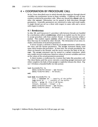
![209
begin -- body of BoundedBuffer 12
loop -- each iteration accepts one call 13
select 14
when InCount - OutCount > 0 => 15
accept GetBuffer(Answer) do 16
Answer := 17
Buffer[OutCount mod Size]; 18
return; 19
OutCount := OutCount + 1; 20
end; -- accept 21
or 22
when InCount - OutCount < Size => 23
accept PutBuffer(What) do 24
return; 25
Buffer[InCount mod Size] := What; 26
InCount := InCount + 1; 27
end; -- accept 28
end; -- select 29
end; -- loop 30
end; -- BoundedBuffer 31
BoundedBuffer is a task, that is, a module that contains a thread. Ada sepa-
rates the specification (lines 1–4) from the implementation (lines 5–31). This
module would be declared in the same block as a producer and a consumer
module. The entry declarations in lines 2–3 (repeated in lines 10–11) provide
procedurelike headers that clients of this module may call.
Each of the alternatives in the select statement (lines 14–29) is headed
by a Boolean guard. When BoundedBuffer executes the select command, the
guards are evaluated. Those that evaluate to true dictate which branches
are open. BoundedBuffer is then blocked until a client invokes a procedure
accepted by one of the open branches. If more than one client has already in-
voked such a procedure, then select is nondeterministic; one branch is arbi-
trarily chosen. It is up to the implementation to attempt to be fair, that is,
not to always prefer one branch over another.
The accept statements (lines 16–21 and 24–28) introduce new name
scopes in which the formal parameters are defined. A client remains blocked
until the rendezvous is finished or the server executes return (lines 19 and
25). I have placed the return statements as early as possible to allow the
client to proceed with its own activities.
There is no danger that InCount and OutCount will be simultaneously ac-
cessed by several threads, because they are not shared variables. Only
BoundedBuffer itself can access them. By the same token, it is not possible
for two rendezvous to be active simultaneously. Therefore, rendezvous have
less parallelism than can be obtained by, for instance, event counts.
Copyright Addison-Wesley. Reproduction fee $.02 per page, per copy.
4 COOPERATION BY PROCEDURE CALL](https://image.slidesharecdn.com/advancedprogramminglanguagedesign-230706034617-464d64c2/85/Advanced_programming_language_design-pdf-217-320.jpg)
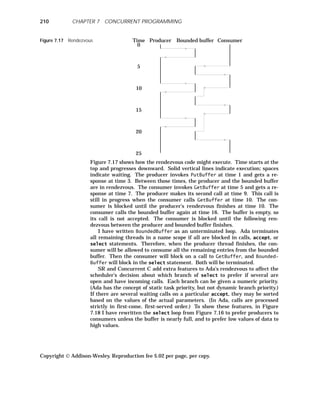
![211
Figure 7.18 select 1
priority -- high number is better 2
if Size - (InCount - OutCount) < 2 3
then 1 else 0 4
accept GetBuffer(Answer) 5
when InCount - OutCount > 0 6
do 7
Answer := Buffer[OutCount mod Size]; 8
return; 9
OutCount := OutCount + 1; 10
end; -- accept 11
or 12
priority -- high number is better 13
if Size - (InCount - OutCount) < 2 14
then 0 else 1 15
accept PutBuffer(What) 16
when InCount - OutCount < Size 17
sortedby (-What) -- prefer low values 18
do 19
return; 20
Buffer[InCount mod Size] := What 21
InCount := InCount + 1; 22
end; -- accept 23
end; -- select 24
The priority clauses (lines 2–4, 13–15) decide which branch to prefer if sev-
eral are open. In this case, the second branch has higher priority unless the
buffer is nearly full. I have placed the when guard (lines 6, 17) after the ac-
cept clause so that the guard can take advantage of the formal parameters
introduced by accept, even though this example doesn’t do so. (SR uses this
order.) The sortedby clause (line 18) reorders multiple calls to PutBuffer
based on the formal parameter What.
4.2 Remote Procedure Call (RPC)
If threads do not share variables (for example, if they are running on differ-
ent machines connected by a network), the only way they can cooperate is by
procedure call or messages. Rendezvous is one way of accepting procedure
calls. The only calls that are handled are those that match open accept
statements. Remote procedure call (RPC) means an invocation that is
handled not by accept statements, but by an ordinary exported procedure.
Such calls can cross compilation units, processes, computers, and even pro-
grams that are written at different times in different languages.
The model of computation for remote procedure calls is somewhat differ-
ent from what I have been discussing so far. Each address space may have
multiple threads, which may share variables in that address space, subject to
any scope rules the language imposes. Threads in separate address spaces do
not share variables.
A thread may invoke an exported procedure inside another address space
by a remote procedure call. There are two equivalent ways to picture the ef-
fect of such a call. You can imagine the thread migrating temporarily to the
address space of the server, performing the call there, and then returning to
Copyright Addison-Wesley. Reproduction fee $.02 per page, per copy.
4 COOPERATION BY PROCEDURE CALL](https://image.slidesharecdn.com/advancedprogramminglanguagedesign-230706034617-464d64c2/85/Advanced_programming_language_design-pdf-219-320.jpg)
![the client’s address space. Address spaces thus share information by sending
their threads to visit other address spaces, bringing and returning data in
their parameters. Alternatively, you can imagine the calling thread sending a
message to the server and then blocking. A new service thread starts in the
server address space for the purpose of handling the call. When it finishes, it
sends results back to the blocked client thread, causing the client to awaken.
The service thread then terminates. The first view is simpler. The underly-
ing implementation is likely to use something closer to the second view.
In the DP (Distributed Processes) language of Brinch Hansen
[Brinch Hansen 78], each address space starts with one thread, which starts
running the main program of that address space. That thread cannot create
new threads, but it may wait for conditions (using an await statement). Re-
mote procedure calls are blocked until no thread is active in the server. A
thread is considered inactive if it has terminated or if it is blocked waiting for
a condition. It is active, however, if it is in the middle of a remote procedure
call to some other address space. Therefore, the programmer does not need to
be afraid that variables will suddenly have different values after a remote
procedure call returns; such a call is indivisible. An await relaxes exclusion,
though, allowing a client thread to visit. Therefore, data can change during
await, but await checks a Boolean condition that can prevent it from un-
blocking until the situation is appropriate.
Figure 7.19 is an implementation of a bounded buffer in DP.
Figure 7.19 -- declarations as in Figure 7.4 (page 192). 1
procedure PutBuffer(value What : Datum); 2
begin 3
await InCount - OutCount < Size do 4
Buffer[InCount mod Size] := What; 5
InCount := InCount + 1; 6
end; -- region 7
end -- PutBuffer; 8
procedure GetBuffer(result Answer : Datum); 9
begin 10
await InCount - OutCount < Size do 11
Answer := Buffer[OutCount mod Size]; 12
OutCount := OutCount + 1; 13
end; -- region 14
end GetBuffer; 15
This code is remarkably similar to Figure 7.4 (page 192). The only difference
is that there is no need to lock any mutexes, since the thread executing either
PutBuffer or GetBuffer is guaranteed exclusion in any case.
Languages like C that do not have remote procedure call built in can take
advantage of a stub compiler, which takes a specification of the exported
procedures and builds suitable code for both the client and the server
[Nelson 81]. One widely available stub compiler is Sun RPC, a remote-
Copyright Addison-Wesley. Reproduction fee $.02 per page, per copy.
212 CHAPTER 7 CONCURRENT PROGRAMMING](https://image.slidesharecdn.com/advancedprogramminglanguagedesign-230706034617-464d64c2/85/Advanced_programming_language_design-pdf-220-320.jpg)
![213
procedure-call library designed by Sun Microsystems, Inc.2
This library in-
cludes procedures for both the client (c) and server (s) for establishing a con-
nection between them (c and s), sending a remote procedure call (c), receiving
a remote procedure call (s), sending a response (s), and receiving the response
(c). Parameters are transmitted in both directions in a machine-independent
data format called “External Data Representation” (XDR); the client and
server must call conversion routines to package and unpackage parameters to
and from this format.
Many experimental languages have been designed to offer RPC directly,
without explicit recourse to library packages. They all offer some mechanism
for establishing a connection between a client and server, typically involving
search through some name space (so the client can find a server) and connect-
ing to some interface (to make sure the client and the server agree on what
calls are valid). They might provide synchronization methods based on any of
the methods I have described earlier to control access to variables that are ac-
cessed by multiple threads in the same address space. They often include au-
tomatic transmission of structured parameters. Argus even allows the
parameters to contain pointer types. The runtime routines expand such val-
ues for transmission by traversing all the pointers. Argus also supports re-
mote invocation of CLU iterators and lets the invoked procedure raise
exceptions.
The compiler sees to it that remote procedure calls are packaged into mes-
sages in the client and unpackaged in the server by using a stub compiler. It
also tries to ensure that RPC is type-secure, that is, that the procedure
header in the server matches the call that the client is making. One mecha-
nism for type security is to represent the type of the procedure (that is, its
name and the types and modes of its parameters) as a string and then to de-
rive a hash value from that string [Scott 88]. These hash values can be com-
piled; they need not be computed at runtime. The hash value is sent in each
call message from client to server. The server checks that the hash value is
correct; if not, there is a type error. A related idea is to represent each type
as a tree, derive a polynomial from the tree, and evaluate the polynomial at a
special point to produce a hash value [Katzenelson 92].
4.3 Remote Evaluation (REV)
Remote procedure call only works if the server exports the procedure that the
client needs. But clients are often written long after the server, and they may
have needs that were not foreseen in the server. Some clients may need the
server to run specialized procedures that most clients would not be interested
in but which could run far more efficiently on the server than on a client, be-
cause the client would need to repeatedly invoke server routines remotely.
Remote evaluation (REV) is a technique that allows clients to send not
only parameters, but also procedures, to the server [Stamos 90]. The proce-
dures may refer to other procedures exported by the server. For example, a
mail-delivery server might export a procedure DeliverMail. A client that
wants to send a hundred identical messages could use RPC, invoking Deliv-
erMail a hundred times, each time passing the message. Alternatively, it
hhhhhhhhhhhhhhhhhhhhhhhhhhhhhhhhhhhh
2
2550 Garcia Avenue, Mountain View, California, 94043
Copyright Addison-Wesley. Reproduction fee $.02 per page, per copy.
4 COOPERATION BY PROCEDURE CALL](https://image.slidesharecdn.com/advancedprogramminglanguagedesign-230706034617-464d64c2/85/Advanced_programming_language_design-pdf-221-320.jpg)
![could use REV, sending a small procedure to the server that invokes Deliver-
Mail a hundred times. The REV method is likely to be far more efficient. It
also frees the mail-server designer of worries that the set of procedures ex-
ported by the server is not exactly right for every client.
A programming-language implementation of REV must be able to deter-
mine whether the server exports enough operations to support an REV re-
quest; if not, it must decide how much code actually needs to be sent. At one
extreme, the procedure that is to be evaluated is itself exported by the server.
In that case, the client needs to send only the parameters and receive the re-
sults; REV becomes RPC. At the other extreme, not only does the server not
export the procedure, but several other procedures that it calls in turn are
also not exported. The client must bundle and send enough procedures to en-
sure that the server will be able to complete the REV request. Any nonlocal
variables needed by those procedures must also be bundled, and they must be
returned by the server to update the values in the client.
The client can bundle the procedures needed by an REV request either at
compile time or runtime. Compile-time bundling is more efficient but more
restrictive. To make a compile-time bundle, the compiler must know what
procedures are exported by the server, and it must traverse the invocation
graph of the invoked procedure to discover all the procedures that must be in-
cluded. To make a runtime bundle, the compiler must prepare the invocation
graph and keep it until runtime. When an REV request is encountered, the
client must query the server to discover its list of exported procedures and
traverse the invocation graph.
REV requests may be nested. A procedure that is sent from a client to a
server may contain another REV request to some other server. Compile-time
bundling is unlikely to work for nested requests, because the contents of the
nested bundle depend on the invocation graph in the server, which is not nec-
essarily available to the compiler of the client.
REV requests that pass procedures as parameters cause a special prob-
lem. Compile-time bundling might refuse to deal with such parameters un-
less their binding is known at compile time.
REV can cause a major security headache. The server must be protected
against misbehaving procedures that are sent to it. Authentication protocols
can be used to restrict clients to those on an approved list. Running the pro-
cedure in a separate thread on the server under some sort of time slicing can
protect the server against wasting all its time on a nonterminating computa-
tion. Giving that separate thread readonly access to server variables can pro-
tect the server against data corruption, but it restricts REV to operations that
do not need to modify server data. Interpreting the REV request in the
server instead of running it can allow the server to refuse potentially danger-
ous operations.
REV can be made implicit in every call and divorced from language de-
sign. The language runtime support can choose on every RPC whether to im-
plement the request by sending a message for RPC, sending a bundle for
REV, or requesting a bundle from the server for local evaluation. This deci-
sion can be based on statistics gathered during execution in an attempt to
balance communication and computational resources among machines
[Herrin 93]. The contents of the bundle need not include more than the pro-
cedure mentioned in the RPC; there is no need either at compile time or run-
Copyright Addison-Wesley. Reproduction fee $.02 per page, per copy.
214 CHAPTER 7 CONCURRENT PROGRAMMING](https://image.slidesharecdn.com/advancedprogramminglanguagedesign-230706034617-464d64c2/85/Advanced_programming_language_design-pdf-222-320.jpg)
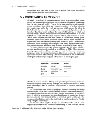
![tion machine(s) receives it, until the destination thread(s) receives it, or until
a response arrives back to the sender from the destination thread(s). Seman-
tics that do not wait for the destination machine are usually called asyn-
chronous, and those that wait for a response are called synchronous. There
is a wide spectrum of synchronicity, so these terms are not very precise. The
data that are sent can be treated just as an array of characters, or they may
have associated type information.
The receive operation is used to accept incoming messages. It may be se-
lective; that is, it might only accept messages that arrive on a set of connec-
tions or messages that match some pattern. It might reorder messages based
on their contents. It might block until such a message arrives; it may have a
timeout period, after which it fails if no message arrives; or it may just enable
a receive but allow the thread to continue executing other statements.
The reply operation sends data back to the originator of the most recent
message. In some languages, such as SR and Hermes, the program can spec-
ify which message is being responded to, so replies need not follow the order
of receives. Packages that provide reply often have a single operation that
combines send and receive. The client uses send/receive and the server
uses receive followed by reply.
The forward operation redirects the most recent incoming message (or a
specified message) to a different destination. The recipient can then reply di-
rectly to the original sender. This facility is called delegation.
5.1 CSP
CSP (Communicating Sequential Processes) is a proposal made by
C. A. R. Hoare for message passing between threads that do not share vari-
ables [Hoare 78]. It is the framework upon which Occam was developed
[May 83]. Communication is accomplished by send and receive statements.
Although the send statement looks like a procedure invocation, in fact it is a
pattern specification, much like Prolog (discussed in Chapter 8). The pattern
is built out of an identifier and actual parameters. It is matched against a
pattern in a receive statement in the destination thread. Variables in the
receive pattern are like formal parameters; they acquire the values of the ac-
tual parameters in the matching send pattern. Patterns match if the pattern
name and the number of parameters are the same and all formal parameter
patterns match the actual parameter patterns. Matching is even used for the
assignment statements, as in the examples shown in Figure 7.20.
Figure 7.20 left := 3; 1
right := 4; 2
x := cons(left, right); -- assigns pattern "cons(3,4)" 3
form(right) := form(right+1); -- right := right+1 4
factor(cons(left,right)) := factor(cons(5,6)); 5
-- left := 5; right := 6 6
right = imply(); -- pattern with no parameters 7
muckle(left) := mickle(left+1); -- match error 8
Variables can hold pattern values, as in line 3. Here, cons is not a procedure
call, just a pattern constructor. Line 4 shows that matching the actual to the
formal is like an ordinary assignment. Line 5 shows that matching works re-
Copyright Addison-Wesley. Reproduction fee $.02 per page, per copy.
216 CHAPTER 7 CONCURRENT PROGRAMMING](https://image.slidesharecdn.com/advancedprogramminglanguagedesign-230706034617-464d64c2/85/Advanced_programming_language_design-pdf-224-320.jpg)
![217
cursively. Patterns need not have parameters (line 7). If the pattern name
disagrees, match fails (line 8). In each of these cases (except the last), a re-
ceive in one thread with the pattern on the left-hand side would match a
send in another thread with the pattern on the right-hand side.
CSP’s control structures include Ada’s nondeterministic select and also a
nondeterministic while, which iterates open branches until no branch is
open. Guards can be Boolean expressions, but they may also have as a final
condition a send or receive statement. If the guard has such a statement, it
is called an output guard or an input guard. For implementation reasons,
original CSP did not allow output guards. It is hard, but not impossible, for
an implementation to pair communicating threads when several have both
send and receive guards open. Pairing is easier under the restriction that a
guarded send or receive can only be matched with an absolute (unguarded)
receive or send; some implementations of CSP make that restriction and al-
low output guards.
Figure 7.21 shows how a bounded buffer can be implemented in CSP, us-
ing both input and output guards.
Figure 7.21 type 1
Datum = ... -- contents of the buffer 2
thread BoundedBuffer; 3
constant 4
Size = 10; -- capacity of the buffer 5
variable 6
Buffer : array 0..Size-1 of Datum; 7
InCount, OutCount : integer := 0; 8
begin 9
while -- each iteration handles one interaction 10
when InCount - OutCount > 0 and 11
receive PutBuffer(Buffer[InCount mod Size]) 12
from Producer => 13
InCount := InCount + 1; 14
when InCount - OutCount < Size and 15
send TakeBuffer(Buffer[OutCount mod Size]) 16
to Consumer => 17
OutCount := OutCount + 1; 18
end; -- while 19
end; -- thread Buffer 20
thread Producer; 21
begin 22
loop 23
Value := ...; -- generate value 24
send PutBuffer(Value) to BoundedBuffer; 25
end; -- loop 26
end; -- Producer 27
Copyright Addison-Wesley. Reproduction fee $.02 per page, per copy.
5 COOPERATION BY MESSAGES](https://image.slidesharecdn.com/advancedprogramminglanguagedesign-230706034617-464d64c2/85/Advanced_programming_language_design-pdf-225-320.jpg)
![thread Consumer; 28
begin 29
loop 30
receive TakeBuffer(Value) from BoundedBuffer; 31
...; -- use value 32
end; -- loop 33
end; -- Consumer 34
The Producer thread (lines 21–27) repeatedly generates a value and sends it
to the BoundedBuffer thread inside a PutBuffer pattern. This send blocks
Producer if BoundedBuffer is not able to accept the match immediately, ei-
ther because it is occupied with something else or because there is no match-
ing receive currently open. The Consumer thread (lines 28–34) repeatedly
receives a value from BoundedBuffer with a TakeBuffer pattern. This re-
ceive can block Consumer if BoundedBuffer does not have a matching send
currently open. BoundedBuffer spends all its time in a nondeterministic
while loop (lines 10–19) with two branches, one to accept data from Producer
(lines 11–14), and the other to feed data to Consumer (lines 15–18). Each
branch is guarded to make sure that the buffer situation allows it to be se-
lected. The first guard is an input guard, and the second is an output guard.
If the buffer is neither full nor empty, both guards will be open, and
whichever of Producer and Consumer is ready first will match its respective
receive or send statement. If both are ready, then the scheduler will select
one in an arbitrary, but in the long run fair, way. The while will always have
at least one branch open, so it will never terminate.
5.2 Lynx
Lynx is an experimental language implemented at the University of Wiscon-
sin and at the University of Rochester [Scott 84, 86]. Address spaces and
modules in Lynx reflect the structure of a multicomputer, that is, a dis-
tributed-memory machine. Each outermost module represents an address
space. As in DP, each address space begins executing a single thread. That
thread can create new threads locally and arrange for threads to be created in
response to messages from other processes. Threads in the same address
space do not execute simultaneously; a thread continues to execute until it
blocks, yielding control to some other thread. It is not an error for all threads
to be blocked waiting for a message to be sent or received.
Lynx is quite helpful for programming long-running processes (called
server processes) that provide assistance to ephemeral processes (called
client processes). Typically, server processes are programmed to build a
separate thread for each client process to keep track of the ongoing conversa-
tion between server and client processes. That thread may subdivide into
new threads if appropriate. Lexical scope rules determine what variables are
visible to any thread; the runtime organization uses a cactus stack.
Lynx provides two-way communication links as first-class values. A link
represents a two-way channel between address spaces. The program dynami-
cally binds links to address spaces and entries. Links can be used for recon-
figurable, type-checked connections between very loosely coupled processes
that are designed in isolation and compiled and loaded at disparate times.
Copyright Addison-Wesley. Reproduction fee $.02 per page, per copy.
218 CHAPTER 7 CONCURRENT PROGRAMMING](https://image.slidesharecdn.com/advancedprogramminglanguagedesign-230706034617-464d64c2/85/Advanced_programming_language_design-pdf-226-320.jpg)
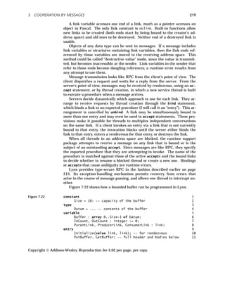
![procedure PutBuffer(value What : Datum); 12
begin 13
Buffer[InCount mod Size] := What; 14
InCount := InCount + 1; 15
if InCount - OutCount = 1 then -- no longer empty 16
bind ConsumerLink to GetBuffer; 17
end; 18
if InCount - OutCount = Size then -- now full 19
unbind ProducerLink from PutBuffer; 20
end; 21
end -- PutBuffer; 22
procedure GetBuffer(result Answer : Datum); 23
begin 24
Answer := Buffer[OutCount mod Size]; 25
OutCount := OutCount + 1; 26
if InCount - OutCount = 0 then -- now empty 27
unbind ConsumerLink from GetBuffer; 28
end; 29
if InCount - OutCount = Size-1 then -- no longer full 30
bind ProducerLink to PutBuffer; 31
end; 32
end; -- GetBuffer 33
begin -- main 34
accept Initialize(ProducerLink, ConsumerLink) 35
on ParentLink; 36
bind ProducerLink to PutBuffer; 37
end; -- main 38
The program defines three entries (lines 9–11); one is for rendezvous, and the
others are handled by thread creation. This program begins with one thread
that executes accept (lines 35–36) to get values for the links to the producer
and consumer. It gets these values in a startup message from its parent, to
which it is connected by ParentLink. I ignore how ParentLink gets initial-
ized. Then the program binds ProducerLink (line 37) to its entry PutBuffer.
It makes no sense to bind ConsumerLink yet, because there is nothing yet to
consume. Then the main thread terminates. Incoming RPC will create new
threads as needed. Both PutBuffer and GetBuffer arrange for binding and
unbinding entries when the buffer gets full, empty, or no longer full or empty
(lines 16–21 and 27–32). PutBuffer and GetBuffer themselves do not need to
block if the buffer is not ready for them, because the pattern of bindings and
the nonpreemptive scheduler assure that they cannot be called unless the
state of the buffer permits them to proceed.
5.3 Linda
Like CSP, Linda also uses patterns instead of procedure calls in its messages
[Gelernter 85]. Unlike CSP, the send statement does not indicate the thread
to which data are to be sent, nor does receive indicate from which thread the
data are coming. Instead, send places the data in a global data pool that can
be accessed by any thread, and receive takes data from that pool. It is up to
the implementation to organize data so that threads running on multiple ma-
Copyright Addison-Wesley. Reproduction fee $.02 per page, per copy.
220 CHAPTER 7 CONCURRENT PROGRAMMING](https://image.slidesharecdn.com/advancedprogramminglanguagedesign-230706034617-464d64c2/85/Advanced_programming_language_design-pdf-228-320.jpg)
![221
chines can find data in the global pool. Typically, implementations will hash
on the pattern name3
and store each bucket redundantly on n1/2
out of n ma-
chines. The receive pattern can include parameters that are variables (like
actual parameters in result mode, to be bound to values during matching),
constants (to selectively receive by restricting what data match this pattern),
and don’t-cares. Receive blocks the caller until matching data appears in the
pool, and then it indivisibly removes the matching data from the pool. There
is also a read statement with the same semantics as receive except that the
data are not removed from the pool.
A Linda implementation of the bounded buffer would be identical to the
CSP one in Figure 7.21 (page 217), except that the send and receive state-
ments would not indicate which thread was the intended partner. Multiple
producers and consumers could use the same code. However, such a bounded
buffer thread would be illogical in Linda, since the data pool itself is an un-
bounded buffer. Even if the bounded buffer is full, the producer would still be
able to repeatedly send the PutBuffer pattern. It would be more straightfor-
ward for the producer to just send a BufferData pattern and for the con-
sumer to receive that pattern. A truly bounded buffer can actually be
implemented in Linda; see the exercises for details.
The advantage of the Linda approach is that programs need not consider
the destination and synchronization aspects of each message that is passed.
If a particular destination thread is important, that can be coded into the pat-
tern, of course, but many applications will not need such explicit control.
One set of applications to which Linda is well suited involves problems
whose solutions create subproblems. All problems are placed in a “problem
heap” as they are generated. The heap is stored in the global pool. Each
thread repeatedly extracts a problem (using receive) and solves it, putting
any new subproblems back on the heap (using send). This situation is much
like a bounded buffer, but there is no concept of order connecting the ele-
ments of the buffer.
Linda is generally implemented as a library package added to some other
language, such as C. A more type-safe design called Lucinda, which combines
Linda with Russell, has also been devised [Butcher 91].
5.4 SR
The SR language was developed over a period of ten years by Gregory An-
drews at the University of Arizona [Andrews 88]. It contains features for
both distributed- and shared-memory concurrency.
SR modules are separately compiled. A module specification and its body
may be compiled separately. At runtime, modules are dynamically instanti-
ated and given initial actual parameters. By default, a new module shares
the address space of its creator, but it can be placed on any machine (physical
or virtual) instead.
Ordinary modules may import declaration modules. Each declaration
module may import other declaration modules and introduce constants,
hhhhhhhhhhhhhhhhhhhhhhhhhhhhhhhhhhhh
3
What I call the pattern name would actually be the first element of a tuple in Linda, but I
find CSP nomenclature a bit easier to understand.
Copyright Addison-Wesley. Reproduction fee $.02 per page, per copy.
5 COOPERATION BY MESSAGES](https://image.slidesharecdn.com/advancedprogramminglanguagedesign-230706034617-464d64c2/85/Advanced_programming_language_design-pdf-229-320.jpg)
![types, variables, entries, and procedures. These may appear in any order, so
dynamic-sized arrays are easy to build. Declaration modules also have ini-
tialization code. The declaration modules are instantiated (at most once
each) and initialized at runtime in whatever order is dictated by the partial
order of imports. One copy is created dynamically per address space the first
time it is needed, so that threads in each space have access to the declara-
tions. Global variables imported from declaration modules should be treated
as readonly; modifying a global variable only affects the copy in the current
address space.
SR contains a wide variety of synchronization and communication meth-
ods. It provides synchronization by semaphores (implemented as a module
type with entries for up and down), and communication by rendezvous, RPC,
and messages. The client may choose whether to use synchronous or asyn-
chronous calls, that is, RPC or messages. The server may choose to receive
messages by thread creation or by rendezvous. It may inspect how many
calls are outstanding on any entry. The rendezvous accept statement4
in-
cludes both a synchronization (when) clause and a scheduling (sortedby)
clause, both of which may depend on the formal parameters of the call. Both
a reply and a forward statement are included.
Destinations for calls can be represented by pointers to modules, which
can even reference modules across machine boundaries. The declaration for
module pointers includes which module type they may reference. Every mod-
ule instance has a pseudovariable self that points to itself. Calls and replies
may pass module pointers, so communication paths may vary dynamically. In
addition, threads may invoke an entry imported from a declaration module.
Any module instance that imports that declaration module may receive such
an invocation.
In addition to initialization code, a module can be contain a thread decla-
ration, much as in Modula. The compiler converts that declaration to an
anonymous entry with no parameters; the act of instantiating the module im-
plicitly sends a message to that entry, which creates the new thread. A mod-
ule may also contain finalization code, which is invoked in any instance when
the instance is terminated. All instances are terminated when deadlock oc-
curs, as in Ada.
5.5 Object-Oriented Programming
The object-oriented paradigm (see Chapter 5) lends itself nicely to dis-
tributed-memory machines, because each object may reside entirely within a
single memory, and interaction between that object and the rest of the compu-
tation is entirely mediated by messages. There are several object-oriented
languages for concurrent programming. For example, DC++ is a version of
C++ with threads [Carr 93], Distributed Eiffel [Gunaseelan 92] and Eiffel
Linda [Jellinghaus 90] extend the object-oriented Eiffel language, and CST
(Concurrent Smalltalk) extends Smalltalk [Dally 89]. You can read a survey
of these languages and others in [M. Nelson 91].
hhhhhhhhhhhhhhhhhhhhhhhhhhhhhhhhhhhh
4
I am changing the keywords, as usual, for the sake of consistency.
Copyright Addison-Wesley. Reproduction fee $.02 per page, per copy.
222 CHAPTER 7 CONCURRENT PROGRAMMING](https://image.slidesharecdn.com/advancedprogramminglanguagedesign-230706034617-464d64c2/85/Advanced_programming_language_design-pdf-230-320.jpg)
![223
To show you a concrete example, I will focus on the ALBA language
[Hernández 93], another example of an object-oriented concurrent program-
ming language. ALBA is strongly typed and is in many ways a typical object-
oriented language; that is, it provides classes and inheritance. What sets it
apart is its recognition that it executes in a distributed environment. Unfor-
tunately, the ALBA document is incomplete, so I have added further specifi-
cations of my own that the authors may not agree with.
There are no class variables, because different instances of a class are
likely to be in different memories. Instance variables, of course, exist. Any
number of threads may simultaneously execute methods in an object unless
the object is an instance of a serialized class, which allows only one thread
at a time. It is unclear whether serialized ALBA objects accept new threads
when the existing thread is blocked waiting for a call or when the existing
thread is in the middle of invoking a method in some other object.
Objects may be created at any time; their identity is stored in an instance
variable of their creator, so that the creator can send them messages. This
identity can be passed to other objects in a parameter in order to allow them
to invoke methods in the newly created object. Each object has a pseudovari-
able creator that points to the creator and self that points to itself.
When an object is created, the programmer has some control over where it
will be placed initially. The ALBA implementation does not dynamically
move objects once they are created, but techniques for such migration are
well understood [Artsy 89]. The class declaration may restrict its instances to
a subset of the machines, and the instance-creation request may further re-
strict the positioning. For this purpose, ALBA has a data type for sets of ma-
chine identifiers.
As in Ada, Lynx, and SR, ALBA objects can accept incoming messages by
rendezvous. Alternatively, an invocation of a method may be handled by
thread creation.
During execution of a method, two more pseudovariables are defined:
sender and reply. Typically, they are identical, pointing to the object that in-
voked the method. However, ALBA provides for delegation. A method may
be invoked with an explicit “reply-to” specification, which will be copied to the
recipient’s reply pseudovariable.
Figure 7.23 shows an ALBA implementation of merge sort.
Figure 7.23 type 1
DataArray = array whatever of integer; 2
class MergeSort; 3
method Done -- for rendezvous 4
(Sorted : DataArray; LowIndex, HighIndex : Integer); 5
method Sort -- thread-creating 6
(Tangled : DataArray; LowIndex, HighIndex : integer); 7
variable 8
MidPoint : integer := (LowIndex + HighIndex) div 2; 9
LeftChild, RightChild : MergeSort; 10
Responses : integer := 0; 11
Copyright Addison-Wesley. Reproduction fee $.02 per page, per copy.
5 COOPERATION BY MESSAGES](https://image.slidesharecdn.com/advancedprogramminglanguagedesign-230706034617-464d64c2/85/Advanced_programming_language_design-pdf-231-320.jpg)
![begin -- method Sort 12
if LowIndex + 1 < HighIndex then -- worth sorting 13
MidPoint : integer := (LowIndex + HighIndex) div 2; 14
create LeftChild; 15
create RightChild; 16
send LeftChild.Sort(Tangled, 1, MidPoint); 17
send RightChild.Sort 18
(Tangled, MidPoint+1, HighIndex); 19
while Responses < 2 do 20
accept Done(Sorted, LowIndex, HighIndex) 21
from {LeftChild, RightChild} 22
do 23
Tangled[LowIndex .. HighIndex] := 24
Sorted[LowIndex .. HighIndex]; 25
Responses := Responses + 1; 26
end; -- accept 27
end -- while 28
Merge(Tangled, 1, MidPoint, MidPoint+1, 29
HighIndex); 30
end; -- worth sorting 31
send creator.Done(Tangled, 1, HighIndex); 32
destroy(self); 33
end; -- method Sort 34
end; -- class MergeSort 35
A client that wishes to sort an array creates an instance of MergeSort (I will
call it the “worker”) and invokes the thread-creating Sort method (lines
6–34). Because objects do not share memory, all parameters to Sort are
passed in value mode. The worker creates left and right child instances (lines
15–16); they are declared in line 10. The worker then invokes the Sort
method in the children on the appropriate regions of the array (lines 17–19).
These calls are marked send to indicate that the call is asynchronous; that is,
the caller need not wait for a response. Asynchronous calls are only allowed
on methods that do not return values. When the children are finished, they
will invoke the Done method in their creator, the worker. The worker accepts
these invocations in a rendezvous (lines 21–27), placing the result that comes
with the invocation back into a slice of the local array (lines 24–25). When it
has received both responses, the worker merges the two halves of the array
(lines 29–30). It then tells its own creator that it is done (line 32), providing
the sorted array as a parameter. This invocation of Done is asynchronous, but
it does not create a new thread, because it is accepted in a rendezvous by the
creator. The worker then destroys its instance (line 33), including all threads
that may currently be active. Its purpose has been accomplished.
ALBA supports multicast by letting a program asynchronously invoke a
non-value-returning method on any subset of the existing instances of a class.
The destination of an invocation can be an instance (the usual case), a set of
instances, or a class (all existing instances are sent the message). Ren-
dezvous can be selective by restricting attention to messages from a given in-
stance, a set of instances, or a class. In line 22, I have restricted attention to
the two children, although such a restriction is not necessary.
Copyright Addison-Wesley. Reproduction fee $.02 per page, per copy.
224 CHAPTER 7 CONCURRENT PROGRAMMING](https://image.slidesharecdn.com/advancedprogramminglanguagedesign-230706034617-464d64c2/85/Advanced_programming_language_design-pdf-232-320.jpg)
![225
5.6 Data-Parallel Programming
Scientific applications often require similar computations across very large
data sets, which may represent a connected physical entity. For example, a
weather simulator might advance time in small increments while keeping
track of wind patterns, cloud cover, precipitation, sunlight-induced wind cur-
rents, and so forth over a large geographical area represented as intercon-
nected records, each covering a few square miles. Such applications often
strain the computational ability of any single computer, so they are pro-
grammed on shared-memory or distributed-memory computers. Each com-
puter is given a region of the data and computes as independently as possible
of the other computers. When necessary, computers exchange information
with others that deal with neighboring data. This style of computing is called
data-parallel computing with coarse-grain parallelism. That is, the ma-
chines work in parallel on different parts of the data, and they only coordi-
nate their activities on occasion.
Several languages have been implemented specifically to deal with coarse-
grain parallelism. Some, like PVM [Sunderam 89], are implemented as li-
brary packages to be invoked from any conventional language for passing
messages. Charm is a more complex language that extends C with dynami-
cally creatable threads that inhabit modules [Kalé 90]. Global variables can
be accessed only by a runtime procedure because they may be stored any-
where. The threads communicate both by messages (much like method invo-
cations in object-oriented programming) and through serialized modules that
accumulate data, creating such results as sums and averages.
The Canopy language is more complex yet. It is implemented as a library
package to be used by ordinary C programs. Unlike PVM and Charm, it im-
poses a distinctively data-parallel view on the programmer.
Data in Canopy are represented as records stored on a grid of sites. Grids
are dynamically constructed by calls to a runtime routine. Definition rou-
tines are provided for many standard topologies, such as three-dimensional
meshes, and the programmer may define any desired topology by using a
more primitive routine. A computation may use several different grids, al-
though using more than one is unusual. Each site in a grid has coordinates
and is connected to its neighbors by links. Data records are associated with
each site and each link.
The runtime support software arranges for sites to be located on physical
machines. Typically, there are far more sites than machines; a typical prob-
lem may have a million sites running on a hundred machines. The program-
mer has no control over the mapping of sites to machines, and there is no way
for a program to discover that mapping. Each machine has a complete copy
of all code and global data and has space to allocate site-local data.
Computation proceeds in phases. Each phase is initiated by a distin-
guished site called the controller, which executes the control program. Before
the first phase, the controller establishes the grids, site sets, mappings be-
tween grids, and record fields (local variables) that will be used. It then calls
CompleteDefinitions to activate these definitions. For each phase, the con-
trol program may initialize global variables by broadcasting a copy to all sites
(actually, to all machines). Individual sites should treat such global data as
readonly. The controller then invokes a procedure on each site in a grid or
subset of a grid by calling DoTask. Each such site gets its own thread to exe-
Copyright Addison-Wesley. Reproduction fee $.02 per page, per copy.
5 COOPERATION BY MESSAGES](https://image.slidesharecdn.com/advancedprogramminglanguagedesign-230706034617-464d64c2/85/Advanced_programming_language_design-pdf-233-320.jpg)
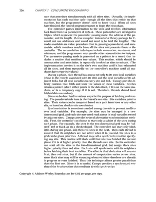
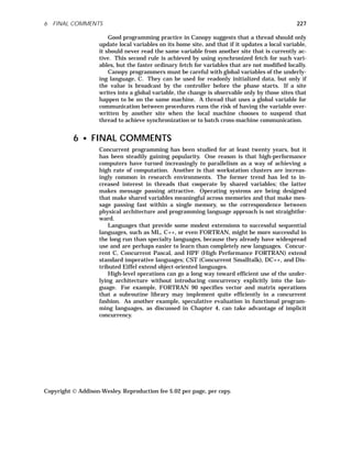
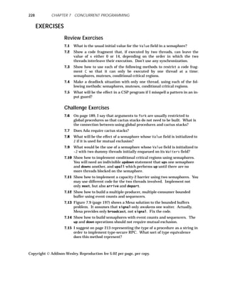

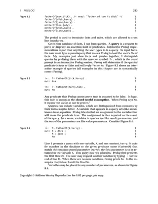
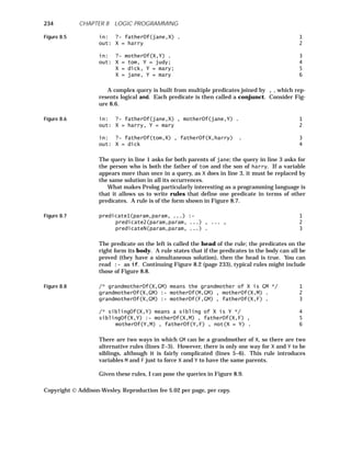
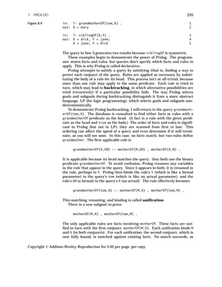
![Prolog backtracks to the point where the first grandmotherOf rule was se-
lected and tries the second rule instead. Unifying the query and the second
grandmotherOf rule gives rise to the new subgoal
motherOf(F,X) , fatherOf(tom,F) .
This subgoal can be satisfied with F = dick and GM = mary. If the second rule
had failed, the entire query would have failed, since no other rules apply.
The backtrack tree of Figure 8.10 shows these steps in more detail.
Figure 8.10 goal: grandmotherOf(tom,X) 1
rule: motherOf(M,X), motherOf(tom,M) 2
fact: motherOf(tom,judy) [M = tom, X = judy] 3
goal: motherOf(tom,tom) 4
fail 5
fact: motherOf(dick,mary) [M = dick, X = mary] 6
goal: motherOf(tom,dick) 7
fail 8
fact: motherOf(jane,mary) [M = jane, X = mary 9
goal: motherOf(tom,jane) 10
fail 11
fail 12
rule: motherOf(F,X), fatherOf(tom,F) 13
fact: motherOf(tom,judy) [F = tom, X = judy] 14
goal: fatherOf(tom,tom) 15
fail 16
fact: motherOf(dick,mary) [F = dick, X = mary] 17
goal: fatherOf(tom,dick) 18
succeed 19
succeed; F = dick, X = mary 20
succeed; X = mary 21
I have bound all identifiers based on the unification steps so far. For exam-
ple, in lines 2 and 13 I have changed GM to X.
The Prolog unification algorithm can be fooled by having it unify a vari-
able with a term containing that same variable, as in Figure 8.11.
Figure 8.11 strange(X) :- X = strange(X) . 1
in: ?- strange(Y) . 2
The variable Y in the query is unified with X in the rule in line 1, leading to Y
= strange(Y). The = constraint causes Y to be unified with strange(Y),
which represents a result, but one that cannot be displayed in a finite space.
Prolog will try to print the nonsense result, which begins strange(strange(.
It turns out to be relatively difficult to solve this “occur-check” problem and
prevent such mistaken unification, so most Prolog implementations don’t try.
They do, however, handle the easier situation encountered in Figure 8.12.
Copyright Addison-Wesley. Reproduction fee $.02 per page, per copy.
236 CHAPTER 8 LOGIC PROGRAMMING](https://image.slidesharecdn.com/advancedprogramminglanguagedesign-230706034617-464d64c2/85/Advanced_programming_language_design-pdf-244-320.jpg)
![237
Figure 8.12 yellow(green(X)) :- X=puce . 1
in: ?- yellow(X) . 2
out: X = green(puce) . 3
The query lin line 2 matches the actual parameter X with the formal parame-
ter green(X). Since one X is actual and the other formal, Prolog does not con-
fuse them.
The backtracking algorithm can also be represented by a box model
[Byrd 80]. Each predicate is represented as a box with two inputs and two
outputs, as shown in Figure 8.13.
Figure 8.13 Box
model of a predicate
Fail
Start
Retry
Succeed
Predicate
The first invocation of a predicate enters from the left. If the predicate is sat-
isfied, control continues out to the right. If a different solution is required,
control reenters from the right. If there are no (more) solutions, control exits
to the left.
The logical and of two predicates is formed by joining them together, as in
Figure 8.14.
Figure 8.14 Logical
and of two predicates
Predicate 2
Fail
Start
Retry
Succeed
Predicate 1
The logical or of two predicates is formed by a different combination, shown
in Figure 8.15.
Figure 8.15 Logical
or of two predicates
Predicate 2
Predicate 1
Fail
Start
Retry
Succeed
When control returns from the right in a retry attempt, it goes to whichever
of the two predicates provided the most recent success.
The query grandmotherOf(tom,X) can be represented in Figure 8.16 in a
box model:
Copyright Addison-Wesley. Reproduction fee $.02 per page, per copy.
1 PROLOG](https://image.slidesharecdn.com/advancedprogramminglanguagedesign-230706034617-464d64c2/85/Advanced_programming_language_design-pdf-245-320.jpg)
![Figure 8.16
Retry
Succeed
Fail
Start
grandmotherOf(X,GM)
fatherOf(X,F)
motherOf(X,M)
motherOf(F,GM)
motherOf(M,GM)
The box model shows execution paths and what happens when a goal suc-
ceeds or fails. It doesn’t show variable substitutions, however.
Backtracking examines the backtrack tree by depth-first search, that is, in
a top-down order. The order of alternatives tried when more than one rule or
fact can be applied can have a startling effect on the speed at which a query is
satisfied (or found to be unsatisfiable). Assume that an evaluator must go
through n levels of rules and facts to provide a solution for a query, and that
at each level, it must choose between two alternatives. If the right decision is
made at each point, the evaluator will operate in O(n) time, because only n
decisions are made. However, if the wrong decision is made at each point, it
is possible that O(2n
) time will be required, because there are that many dif-
ferent settings for the decisions. As a result, Prolog programmers tend to sort
rules and introduce other aids I will present shortly to help the evaluator
make the decisions. For example, the rules for grandmotherOf in Figure 8.8
(page 234) can be improved by reordering the bodies, as shown in the exer-
cises. Nonetheless, except in the case of recursive rules (in which an infinite
expansion of rules can occur), the issue is one of speed, not correctness.
1.2 Separating Logic and Control
A well-known textbook on data structures by Niklaus Wirth is titled
Algorithms + Data Structures = Programs [Wirth 76]. This equation defines
the programming model implicit in modern procedural languages. The pro-
gramming task is essentially to design data structures and the algorithms
that manipulate them.
An interesting alternative view is presented by Robert Kowalski in ‘‘Algo-
rithms = Logic + Control’’ [Kowalski 79]. This article proposes a declarative
programming view. The programmer first specifies the logic of an algorithm.
This component specifies what the result of the algorithm is to be. Then the
control component is defined; it specifies how an evaluator may proceed to ac-
tually produce an answer. The logic component is essential because it defines
what the programmer wants the program to generate. The control compo-
nent may be optional, since it controls how fast an answer may be obtained.
This represents a two-tiered approach in which you think first about getting
the correct answer, and then about making the computation sufficiently fast.
Prolog supports this view of programming; its facts and rules are essen-
tially the logic component of a program. The control component is largely
hidden in Prolog’s evaluator, although certain Prolog commands have been
devised to aid an evaluator, as you will see shortly.
Copyright Addison-Wesley. Reproduction fee $.02 per page, per copy.
238 CHAPTER 8 LOGIC PROGRAMMING](https://image.slidesharecdn.com/advancedprogramminglanguagedesign-230706034617-464d64c2/85/Advanced_programming_language_design-pdf-246-320.jpg)
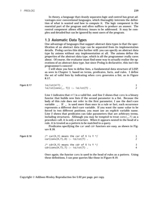
![Figure 8.19 in: ?- car(cons(2,cons(3,nil)),X) . 1
out: X = 2 2
in: ?- car(cons(a,b),X) . 3
out: No 4
in: ?- car(cons(X,nil),2) . 5
out: X = 2 6
in: ?- car(cons(a,X),a) . 7
out: X = nil; 8
X = cons(_1, nil); 9
X = cons(_2, cons(_1, nil)); 10
... 11
The first query (line 1) asks for the car of a particular valid list. The second
(line 3) asks for the car of an invalid list. It fails because the rules only allow
car to be applied to valid lists. The third query (line 5) inverts the question
by asking what has to be consed to a list to obtain a car of 2. The fourth
query (line 7) requests lists whose car is a. There are infinitely many an-
swers. Prolog invents internal temporary names for unbound results, which I
display as _1, _2, and so on (lines 9–10). I call such names don’t-care re-
sults.
In this example, both car and cdr can be used to form queries. However,
cons cannot be used that way; there are no rules with heads matching cons.
In other words, cons is a functor, whereas car and cdr are predicate names.
Stacks are frequently used to illustrate abstract data types, so let me pre-
sent an axiomatic definition of stacks in Figure 8.20.
Figure 8.20 isStack(nil) . 1
isStack(push(_,S)) :- isStack(S) . 2
top(push(Elem,S),Elem) :- isStack(S) . 3
pop(push(_,S),S) :- isStack(S) . 4
in: isStack(push(a,push(b,nil))) . 5
out: Yes 6
in: pop(push(a,push(b,nil)),X) . 7
out: X = push(b, nil) 8
I have used push as a functor, whereas top and pop are predicates. I leave
making pop a functor as an exercise. The Prolog definition of stacks is simi-
lar to that of lists, which shouldn’t be surprising, since lists are often used to
implement stacks in conventional languages. The stacks defined above are
heterogeneous. The exercises explore restricting stacks to hold only integers.
These examples show that Prolog can deal fairly directly with algebraic
specification of data types, a field pioneered by Guttag [Guttag 77]. In the no-
tation of algebraic specification, an integer stack looks like this:
Copyright Addison-Wesley. Reproduction fee $.02 per page, per copy.
240 CHAPTER 8 LOGIC PROGRAMMING](https://image.slidesharecdn.com/advancedprogramminglanguagedesign-230706034617-464d64c2/85/Advanced_programming_language_design-pdf-248-320.jpg)
![241
Figure 8.21 type IntegerStack 1
operations 2
create: → IntegerStack 3
push: IntegerStack × integer → IntegerStack 4
pop: IntegerStack → IntegerStack 5
top: IntegerStack → integer 6
axioms 7
top(create) = error 8
top(push(S,I)) = I 9
pop(create) = error 10
pop(push(S,I)) = S 11
Operations are first defined by naming their input and output types. In pro-
cedural languages, the operations are analogous to the specification part of
an abstract data type. In Prolog, which has no need to distinguish input from
output, the operations can be predicates or functors. Operations that result
in IntegerStacks are called constructors; here, create, push, and pop are
all constructors. Actually, pop is a special kind of constructor because it re-
duces the amount of information; such constructors are called destructors.
Operations that do not result in the abstract data type are called inspectors;
here, top is the only inspector. The axioms are simplification rules. It is not
always easy to see what axioms are needed; a rule of thumb is that an axiom
is needed for all combinations of inspectors and non-destructive constructors
(lines 8 and 9) and all combinations of destructors and non-destructive con-
structors (lines 10 and 11). In Prolog, axioms are expressed as rules, which
means that inspectors (top) and destructors (pop) will be predicates, whereas
non-destructive constructors (push) will be functors.
An algebraic specification could in general be satisfied by many different
models. The axioms equate such elements as create and
pop(push(create,4)), which some models would keep distinct. If only those
elements that the axioms equate are considered equal, the resulting algebra
is called an initial algebra. If all elements are equated that cannot be dis-
tinguished by inspectors, the resulting algebra is called a final algebra. In
the case of stacks, these two algebras are the same. In an algebraic specifica-
tion of arrays, however, the order in which elements are assigned values does
not affect what an inspector returns, so the final algebra is more appropriate
than the initial algebra, which would distinguish arrays with the same ele-
ments that happen to have acquired the elements in a different order.
1.4 List Processing
Because lists are such a familiar and flexible data structure, Prolog provides
a notation for the structures that represent lists. Predefining lists also
makes their manipulation more efficient. Predefined arithmetic operators
are provided for much the same reason. In Prolog, lists are delimited by
brackets. The empty list is [], and [[a,b],[c,d,e]] is a list containing two
sublists (with 2 and 3 elements respectively). The notation [H | T] is used to
represent any list with car H and cdr T, as in Figure 8.22.
Copyright Addison-Wesley. Reproduction fee $.02 per page, per copy.
1 PROLOG](https://image.slidesharecdn.com/advancedprogramminglanguagedesign-230706034617-464d64c2/85/Advanced_programming_language_design-pdf-249-320.jpg)
![Figure 8.22 p([1,2,3,4]) . 1
in: ?- p([X| Y]) . 2
out: X = 1, Y = [2,3,4] 3
in: ?- p([_,_,X| Y]) . 4
out: X = 3, Y = [4] 5
Using this notation, Figure 8.23 defines the list operation append in a manner
analogous to its definition in LISP (actually, append is often predefined).
Figure 8.23 /* append(A,B,C) means C is the list formed by 1
appending element B to the end of list A */ 2
append([],[],[]) . 3
append([],[H| T],[H| T]) . 4
append([X| L1],L2,[X| L3]) :- append(L1,L2,L3) . 5
in: ?- append([1,2],[3,4],S) . 6
out: S = [1,2,3,4] 7
The correspondence to the LISP definition of append is almost exact, except
that no explicit control structure is given. Instead, rules that characterize
append are defined; they allow Prolog to recognize (or build) correctly ap-
pended lists. A LISP-like approach to list manipulation can be used to struc-
ture Prolog rules. Thus I could define a list-membership predicate memberOf
(again, it is often predefined) as shown in Figure 8.24.
Figure 8.24 /* memberOf(X,L) means X is a member of list L */ 1
memberOf(X,[X| _]) . 2
memberOf(X,[_| Y]) :- memberOf(X,Y) . 3
in: ?- memberOf(4,[1,2,3]) . 4
out: No 5
in: ?- memberOf(4,[1,4,3]) . 6
out: Yes 7
This definition is strongly reminiscent of LISP’s tail recursion. However, Pro-
log’s declarative nature allows definitions that are quite foreign to LISP’s pro-
cedural nature. Consider the alternative definition of memberOf in Figure
8.25.
Figure 8.25 memberOf(X,L) :- append(_,[X| _],L) .
This definition says that X is a member of L exactly if there exists some list
that can be appended to a list beginning with X to form list L.
Although both definitions of memberOf are correct, the first one will proba-
bly be more efficiently executed, because it is somewhat more procedural in
flavor. In fact, Prolog definitions are often structured specifically to guide an
evaluator toward a more efficient evaluation of a query. Sorting is a good ex-
ample. The simplest abstract definition of a sort is a permutation of elements
Copyright Addison-Wesley. Reproduction fee $.02 per page, per copy.
242 CHAPTER 8 LOGIC PROGRAMMING](https://image.slidesharecdn.com/advancedprogramminglanguagedesign-230706034617-464d64c2/85/Advanced_programming_language_design-pdf-250-320.jpg)
![243
that puts the elements in nondecreasing (or nonincreasing) order. This defi-
nition has a direct Prolog analogue, shown in Figure 8.26.
Figure 8.26 naiveSort(L1,L2) :- permutation(L1,L2) , inOrder(L2) . 1
permutation([],[]) . 2
permutation(L,[H| T]) :- append(V,[H| U],L) , 3
append(V,U,W) , permutation(W,T) . 4
inOrder([]) . 5
inOrder([_]) . 6
inOrder([A,B| T]) :- A =< B , inOrder([B| T]) . 7
Since a list with n distinct elements has n! permutations, the above definition
may well lead to long and tedious searches in an effort to find a sorting of a
list. An alternative is to define inOrder in a manner that leads to a more effi-
cient evaluation sequence. For example, using the infamous bubble sort
(shame on me!) as inspiration, I create the alternative definition in Figure
8.27.
Figure 8.27 bubbleSort(L,L) :- inOrder(L) . 1
bubbleSort(L1,L2) :- append(X,[A,B| Y],L1), A > B , 2
append(X,[B,A| Y],T), bubbleSort(T,L2) . 3
inOrder([]) . 4
inOrder([_]) . 5
inOrder([A,B| T]) :- A =< B , inOrder([B| T]) . 6
Actually, a trace of execution of bubbleSort will show that it always looks for
and then swaps the first out-of-order pair in the list. There are O(n2
) swaps,
each of which requires O(n) effort to discover by searching from the start of
the list. The result is an O(n3
) algorithm, which is worse than the O(n2
) ex-
pected for bubble sort.
1.5 Difference Lists
List processing can be expensive. The append operation must step to the end
of the first parameter in a recursive fashion before it can begin to construct
the result. Prolog programmers have invented a programming trick called a
difference list to alleviate this problem [Sterling 94]. Each list is repre-
sented in two pieces, which I will call listextra and extra. The actual list is
listextra with extra removed from the end. What extra information to
place at the end of a list is arbitrary and is based on convenience. For exam-
ple, the list [a,b] can be represented in many ways, including [a,b] [] and
[a,b,c,d] [c,d]. In general, I can represent the list as [a,b | Extra] [Ex-
tra] and not specify what Extra might be. The append routine can now be
written as a single, nonrecursive rule, as in Figure 8.28.
Copyright Addison-Wesley. Reproduction fee $.02 per page, per copy.
1 PROLOG](https://image.slidesharecdn.com/advancedprogramminglanguagedesign-230706034617-464d64c2/85/Advanced_programming_language_design-pdf-251-320.jpg)
![Figure 8.28 append(diff(A,B), diff(B,C), diff(A,C)) . 1
in: ?- append(diff([1,2|X],X), diff([3,4|Y],Y), 2
diff(ListExtra,Extra)) . 3
out: X = [3,4|_1], 4
Y = _1, 5
ListExtra = [1,2,3,4|_1], 6
Extra = _1 7
The append predicate defined in line 1 takes three parameters, each of which
is a pattern representing a list in difference-list form. Figure 8.28 shows how
line 1 represents appending two lists by explicitly showing A, B, and C. Lines
2–3 use this definition to append [1,2] and [3,4]. Each of these lists is rep-
resented with a variable (X and Y) to represent the extra parts. Lines 4–5
show how these variables get bound during match. The result is represented
by (ListExtra,Extra), which (according to lines 6–7) is [1,2,3,4|_1] _1. So
long as I am willing to use difference-list form, I have not needed to perform
any recursion.
Figure 8.29 Difference
lists
(A,C)
(B,C)
(A,B)
C
B
A
1.6 Arithmetic
In Prolog, the infix equality predicate = can be used for two purposes. In α =
β, if α and β are both constants, literals, structures, or bound variables, then
the predicate succeeds or fails depending on whether or not the two operands
are identical. Thus 1 = 1 is true, [1,2] = [] is false, and X = 2 is true if X has
been bound to 2. This is the natural interpretation of the equality operator.
However, if α or β (or both) are unbound variables, then α = β succeeds and
binds them together. So the same symbol acts both as an equality operator
and as an assignment operator. Actually, the symbol introduces a constraint.
Figure 8.30 illustrates this point.
Copyright Addison-Wesley. Reproduction fee $.02 per page, per copy.
244 CHAPTER 8 LOGIC PROGRAMMING](https://image.slidesharecdn.com/advancedprogramminglanguagedesign-230706034617-464d64c2/85/Advanced_programming_language_design-pdf-252-320.jpg)
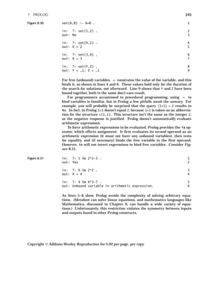
![1.7 Termination Issues
If free variables in queries may be bound only to a finite set of values, a Pro-
log evaluator should be able to prove or disprove any query. However, Prolog
allows recursive definitions (such as the ones I showed earlier for lists and
stacks) that imply infinite domains, as well as primitive objects (such as inte-
gers) with infinite domains. Not all queries will necessarily terminate. Pro-
log specifies that the order in which rules and facts are specified determines
the order in which an evaluator attempts to apply them in proofs. Bad orders
can sometimes lead to an infinite recursion. Suppose that I define the isList
predicate as in Figure 8.32.
Figure 8.32 isList(cons(H,T)) :- isList(T) . 1
isList(nil) . 2
A query like isList(nil) works fine, but isList(X) runs into a real snag.
The top-down evaluator will set X = cons(H,T) and try to prove isList(T).
To do this, it will set T = cons(H′,T′)1
and try to prove isList(T′), and so
forth. Eventually, the evaluator runs out of stack space. Putting the fact is-
List(nil) before the rule solves the problem.
Other problems may arise because of an inadequate set of rules. For ex-
ample, I might provide a definition for odd integers and ask if any odd integer
is equal to 2, as in Figure 8.33.
Figure 8.33 in: odd(1) . 1
odd(N) :- odd(M), N is M + 2 . 2
?- odd(2) . 3
out: [does not terminate] 4
The evaluator never finishes the query in line 3. It keeps generating odd
numbers (1, 3, ...) to match M in line 2, but none of them satisfies 2 is M + 2. It
doesn’t know that after considering 1, all succeeding odd numbers will be
greater than 2 and hence not equal to 2. The query is false, but Prolog has no
mechanism to prove it!
1.8 Resolution Proof Techniques
Prolog is designed to be amenable to a particular class of automatic proof
techniques termed “resolution techniques.” Resolution is a general infer-
ence rule shown in Figure 8.34.
hhhhhhhhhhhhhhhhhhhhhhhhhhhhhhhhhhhh
1
All variable names in a rule are local to that rule; hence, recursive applications cause no
naming conflicts.
Copyright Addison-Wesley. Reproduction fee $.02 per page, per copy.
246 CHAPTER 8 LOGIC PROGRAMMING](https://image.slidesharecdn.com/advancedprogramminglanguagedesign-230706034617-464d64c2/85/Advanced_programming_language_design-pdf-254-320.jpg)
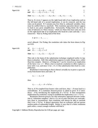
![1.9 Control Aspects
So far I have emphasized the logic component of Prolog. The language also
contains features that exercise control over the evaluation process. Such fea-
tures in general compromise the otherwise declarative nature of Prolog. (Pro-
log also contains I/O, testing, and debugging features that are not purely
declarative.)
The most frequently used control operator is cut (represented by ! in
Prolog syntax). Cut terminates backtracking within a rule. (Cut is similar to
fence in SNOBOL, described in Chapter 9. SNOBOL patterns use a back-
track mechanism that is very similar to the one Prolog uses.) In particular, if
cut is encountered, all alternatives prior to cut in the rule are frozen, as
shown in the box model in Figure 8.36.
Figure 8.36 Cut
operator
Cut Predicate 2
Fail
Start
Retry
Succeed
Predicate 1
Prolog will not try alternative matches to earlier conjuncts of the rule’s body.
In fact, it will not try alternative rules to the rule that contains cut. Consider
Figure 8.37.
Figure 8.37 even(X) :- X=2 , X>0, !, X < 0 . 1
even(X) :- X=10 . 2
in: even(E) . 3
out: No 4
The query in line 3 matches the rule in line 1. The first conjunct binds X to 2,
the second succeeds, but the last conjunct fails. The cut prevents not only a
reevaluation of the first conjuncts (which wouldn’t find anything new in any
case) but also any attempt to use the rule of line 2, which would succeed.
Without the cut operation, Prolog would report that X = 10.
Cut can be useful in cases where once one rule is found to match, it is un-
necessary to try other rules. For example, recall the list membership predi-
cate, memberOf, shown in Figure 8.38.
Figure 8.38 memberOf(X,[X| _]) . 1
memberOf(X,[_| Y]) :- memberOf(X,Y) . 2
Since an element may appear in a list more than once, if a goal containing a
successful memberOf conjunct later fails, Prolog might try to resatisfy it by
looking for an alternative match to memberOf. In general this search will be
futile, since once an item is known to be in a list, backtracking can’t establish
anything new. Thus, we have Figure 8.39.
Copyright Addison-Wesley. Reproduction fee $.02 per page, per copy.
248 CHAPTER 8 LOGIC PROGRAMMING](https://image.slidesharecdn.com/advancedprogramminglanguagedesign-230706034617-464d64c2/85/Advanced_programming_language_design-pdf-256-320.jpg)
![249
Figure 8.39 memberOf(X,[X| _]) :- ! . 1
memberOf(X,[_| Y]) :- memberOf(X,Y) . 2
This code implements our observation that once membership is established,
further backtracking should be avoided. Unfortunately, cut changes the
meaning of the memberOf rule. If the program uses this rule not to verify that
X is a member of some list L but to find a list L with X as a member, cut will
force X to be the first element in L, which prevents other perfectly good lists
from being formed.
Another control operator in Prolog is fail, which always fails; that is, it
can never be proven true. (Again, SNOBOL has an analogous fail pattern.)
A program may use fail to state that a goal can’t be established. For exam-
ple, given a predicate male(X), I might create the rule in Figure 8.40.
Figure 8.40 grandmotherOf(X,GM) :- male(GM) , fail .
This rule states that if GM is male, then GM can’t be anyone’s grandmother. In-
terestingly, this rule doesn’t achieve its intended purpose. The problem is
that backtracking takes effect, saying (in effect) that if this rule doesn’t work,
maybe some other rule will. To avoid backtracking, cut must added, as in
Figure 8.41.
Figure 8.41 grandmotherOf(GM,X) :- male(GM) , ! , fail .
Cut is often used in conjunction with fail when backtracking is to be sup-
pressed. Another use for fail is to create a sort of while loop, as in Figure
8.42.
Figure 8.42 while(X) :- cond(X) , body(X) , fail . 1
cond(X) :- memberOf(X, [1,2,3,7]) . 2
body(X) :- write(X) , write(’ ’) . 3
in: while(_) . 4
out: 1 2 3 7 5
No 6
Other more complex Prolog operators exist. For example, assert and re-
tract can be used to add or remove facts and rules from the database while
evaluation is in progress. These operators can be used to allow a program to
learn, but since they have the flavor of self-modifying code, they are poten-
tially very dangerous.
1.10 An Example of Control Programming
To illustrate some of the subtleties of programming in Prolog, I will consider
the canonical (mis-)example of recursive programming, factorial. The obvious
definition appears in Figure 8.43.
Copyright Addison-Wesley. Reproduction fee $.02 per page, per copy.
1 PROLOG](https://image.slidesharecdn.com/advancedprogramminglanguagedesign-230706034617-464d64c2/85/Advanced_programming_language_design-pdf-257-320.jpg)
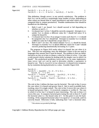
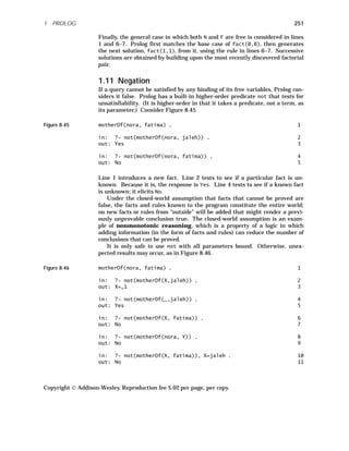
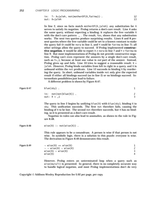
![253
well with it.
1.12 Other Evaluation Orders
Prolog programmers must sort rules to avoid infinite loops. They must also
sort the conjuncts within rules for the sake of efficiency. The naiveSort ex-
ample in Figure 8.26 (page 243) would fail to terminate if line 1 were written
as in Figure 8.50.
Figure 8.50 naiveSort(L1,L2) :- inOrder(L2) , permutation(L1,L2) .
The Prolog interpreter builds more and more fanciful values of L2 that have
nothing at all to do with L1 and fails on each one. Prolog programmers learn
to build rules so that the first conjunct generates potential solutions, and the
remaining conjuncts test them for acceptability. If the generator builds too
many unacceptable results, the rule will be very inefficient.
The fact that rule and conjunct order is so crucial to efficiency detracts
from the declarative nature of Prolog. It would be nice if the rules merely
stated the desired result, and if the implementation were able to dynamically
sort the rules and conjuncts to generate the result efficiently.
One proposal for a different evaluation strategy is found in Specint
[Darlington 90]. A static version of the idea, called “sideways information
passing,” appears in Datalog. The idea is to reorder the conjuncts as they are
satisfied, so that attention is directed to the first conjunct that has not yet
been satisfied. As each conjunct is satisfied, it is rotated to the end of the list
of conjuncts; it may be retested (and resatisfied) later if other conjuncts fail in
the meantime. The programmer can supply hints for each predicate that sug-
gest what parameters will satisfy that predicate. Predefined predicates have
their own hints. For example, Figure 8.51 gives a slightly different version of
naiveSort.
Figure 8.51 naiveSort(L1,L2) :- permutation(L1,L2) , inOrder(L2) . 1
permutation(X,Y) :- X = Y 2
permutation(X| Z,Y) :- delete(X,Y,T) , permutation(Z,T) 3
inOrder([]) . 4
inOrder([_]) . 5
inOrder([A,B| T]) :- A =< B , inOrder([B| T]) . 6
To evaluate naiveSort([1,3,2],result), the evaluator first tries to satisfy
the first conjunct of line 1. This conjunct brings it to line 2 to find an accept-
able permutation Y of X = [1,3,2]. By default, permutation will first try the
empty list for Y. It fails, because it satisfies neither line 2 nor line 3. How-
ever, the equality test of line 2 has a default hint: set Y to X. Now permuta-
tion(X,Y) is satisfied, so the Specint evaluator moves to the inOrder
conjunct of line 1, bringing it to line 6. In line 6, A is 1, B is 3, and T is [2].
The first conjunct succeeds, and inOrder is called recursively on [3,2]. In
the recursive call of line 6, A is 3, B is 2, and T is []. The first conjunct fails.
The hint for satisfying =< is to interchange the two values. Now line 6 suc-
Copyright Addison-Wesley. Reproduction fee $.02 per page, per copy.
1 PROLOG](https://image.slidesharecdn.com/advancedprogramminglanguagedesign-230706034617-464d64c2/85/Advanced_programming_language_design-pdf-261-320.jpg)
![ceeds (after a brief further recursion), and the new values are backed up to
the first instance of line 6. Now A is 1, B is 2, and T is [3]. This instance
rechecks the first conjunct. It was previously satisfied, but values have
changed. Luckily, the new values still satisfy this conjunct. Evaluation re-
turns to line 1. Now L2 is [1,2,3], and the second conjunct is satisfied. The
first conjunct is rechecked. After several instantiations of line 3, this check is
satisfied. Specint ends up with something like insertion sort, using quadratic
time, instead of Prolog’s exponential-time evaluation.
Standard Prolog evaluation starts at the goal and moves to subgoals; this
approach is called top-down evaluation. Another evaluation order that has
been proposed is bottom-up evaluation. In its pure form, bottom-up evalua-
tion would mean starting with facts and deriving consequences, both direct
and indirect. But this sort of undirected evaluation is unlikely to tend toward
the desired goal. Luckily, bottom-up evaluation can be implemented in a
more directed fashion. Given a query, some preprocessing based on the top-
down tree can lead to insight concerning a reasonable ordering of the con-
juncts in the bodies of rules. This insight is based on sideways information
passing, which determines what information is passed in variables between
the conjuncts. The result is a transformed program that can be executed bot-
tom-up. The bottom-up approach leads to certain simplifications. In particu-
lar, the unification algorithm is not needed if every variable that appears in
the head of the rule also appears in its body. This restriction does not seem
unreasonable. Avoiding unification can be essential in some domains. In par-
ticular, strings can be introduced into Prolog with matching rules that match
"abcd" to A + B, matching any initial substring to A and the rest to B. Unifica-
tion is intractable in this setting.
1.13 Constraint-Logic Programming (CLP)
A small extension to Prolog’s evaluation mechanism simplifies programs like
factorial in Figure 8.44 (page 250). This extension, called constraint-logic
programming, or CLP, lets identifiers have a constrained status, which lies
between bound and free [Fruhwirth 92]. CLP(R) is Prolog with constraints
expressed with respect to real numbers.
A conjunct in CLP(R) such as X < 5 is merely checked if X is bound, but if X
is free or constrained, this conjunct introduces a constraint on X. If the new
constraint, in combination with previous constraints, makes a variable unsat-
isfiable, the evaluator must backtrack. The power of this idea can be seen in
Figure 8.52.
Figure 8.52 in: Nice(X, Y) :- X = 6 , Y < 5 . 1
?- Nice(A,B) . 2
out: A = 6, B < 5 3
in: ?- Nice(A,B) , B > 7 . 4
out: No 5
Line 2 is only satisfied by a restricted set of values; the output shows the ap-
plicable constraints. When I add a conflicting constraint in line 4, no results
can be found. Figure 8.53 is a factorial predicate.
Copyright Addison-Wesley. Reproduction fee $.02 per page, per copy.
254 CHAPTER 8 LOGIC PROGRAMMING](https://image.slidesharecdn.com/advancedprogramminglanguagedesign-230706034617-464d64c2/85/Advanced_programming_language_design-pdf-262-320.jpg)
![255
Figure 8.53 fact(N,F) :- N <= 1 , F = 1 . 1
fact(N,F) :- N > 1 , M = N-1 , fact(M,G) , F = N*G . 2
Line 2 does not use the is predicate, because my intent is to introduce a con-
straint, not to perform arithmetic. The query fact(X,Y) elicits the following
solutions:
X ≤ 1, Y = 1
X = Y, 1 < Y ≤ 2.
2 < X ≤ 3, Y = X*(X-1)
3 < X ≤ 4, Y = X*(X-1)*(X-2)
4 < X ≤ 5, Y = X*(X-1)*(X-2)*(X-3)
...
If we add the constraint that all numbers are integers, not arbitrary reals,
then these values reduce to exact solutions. Figure 8.54 computes Fibonacci
numbers.
Figure 8.54 fib(0,1). 1
fib(1,1). 2
fib(N, X1 + X2) :- N > 1 , fib(N - 1, X1) , fib(N - 2, X2) . 3
This program works correctly no matter whether the parameters are free or
bound. Figure 8.55 shows how to multiply two complex numbers.
Figure 8.55 complexMultiply(c(R1, I1), c(R2, I2), c(R3, I3)) :- 1
R3 = R1 * R2 - I1 * I2 , 2
I3 = R1 * I2 + R2 * I1 . 3
The functor c is used as a pattern. We can give CLP(R) queries about com-
plexMultiply, as in Figure 8.56.
Figure 8.56 in: ?- complexMultiply(X, c(2,2), c(0,4)) 1
out: X = c(1,1) 2
in: ?- complexMultiply(X, Y, c(0,0)) 3
out: X = c(A,B), Y = c(C,D), A*C = B*D, A*D = -B*C 4
There are rare occasions when a term someFunctor(3 + 4) is meant to be dif-
ferent from the term someFunctor(4 + 3). CLP(R) allows the programmer to
prevent evaluation of the + operator in such cases by means of a quoting
mechanism.
As a final example of constraint-logic programming, consider the program
of Figure 8.57, which finds the circuits that can be built from two available
resistors in series and a single voltage source so that the drop in voltage
across the second resistor is between 14.5 and 16.25 volts [Jaffar 92]:
Copyright Addison-Wesley. Reproduction fee $.02 per page, per copy.
1 PROLOG](https://image.slidesharecdn.com/advancedprogramminglanguagedesign-230706034617-464d64c2/85/Advanced_programming_language_design-pdf-263-320.jpg)
![Figure 8.57 /* available resistors */ 1
Resistor(10) . 2
Resistor(14) . 3
Resistor(27) . 4
Resistor(60) . 5
Resistor(100) . 6
/* available voltage sources */ 7
Voltage(10) . 8
Voltage(20) . 9
/* electrical law */ 10
Ohm(Voltage, Amperage, Resistance) :- 11
Voltage = Amperage * Resistance . 12
/* query about our circuit */ 13
?- 14.5 < V2, V2 < 16.25 , /* voltage constraints */ 14
Resistor(R1) , Resistor(R2), /* choice of resistors */ 15
Voltage(V) , /* choice of voltages */ 16
Ohm(V1,A1,R1) , Ohm(V2,A2,R2), /* electrical laws */ 17
A1 = A2, V = V1 + V2 . /* series circuit */ 18
An evaluator might choose to solve linear constraints before nonlinear ones in
order to achieve the three solutions.
1.14 Metaprogramming
Chapter 4 shows how a LISP interpreter may be written in LISP. Prolog pro-
vides a similar ability. As with LISP, the trick is to make the language ho-
moiconic, that is, to be able to treat programs as data. Programs are just sets
of rules (a fact is a rule with a body of true). The body of a rule is a comma-
separated list of predicates. In addition to the bracket-delimited lists shown
earlier, Prolog also accepts simple comma-separated lists.3
The head of a rule
is also a predicate, and the :- separator can be treated as an infix binary
predicate.
So a program is a set of predicates, and Prolog provides a way to inspect,
introduce, and delete the predicates that currently make up the program,
that is, to treat the program as data. The clause predicate is used for in-
specting rules, as in Figure 8.58.
Figure 8.58 grandmotherOf(X,GM) :- motherOf(M,GM) , motherOf(X,M) . 1
grandmotherOf(X,GM) :- motherOf(F,GM) , fatherOf(X,F) . 2
hhhhhhhhhhhhhhhhhhhhhhhhhhhhhhhhhhhh
3
Comma-separated lists are the underlying concept. The list a,b,c is equivalent to
a,(b,c). The bracketed list [H | T] is syntactic sugar for the predicate .(H,T), where the dot is
a binary cons functor.
Copyright Addison-Wesley. Reproduction fee $.02 per page, per copy.
256 CHAPTER 8 LOGIC PROGRAMMING](https://image.slidesharecdn.com/advancedprogramminglanguagedesign-230706034617-464d64c2/85/Advanced_programming_language_design-pdf-264-320.jpg)
![257
in: ?- clause(grandmotherOf(A,B),Y). 3
out: A = _1, 4
B = _2, 5
Y = motherOf(_3 _2), motherOf(_1, _3); 6
A = _1, 7
B = _2, 8
Y = motherOf(_3, _2), fatherOf(_1, _3) 9
motherOf(janos,hette) . 10
in: ?- clause(MotherOf(X,Y),Z) . 11
out: X = janos, 12
Y = hette, 13
Z = true 14
Lines 1–2 reintroduce the grandmotherOf predicate that I used before. Line 3
asks for all rules that have a left-hand side matching grandmotherOf(A,B).
This line treats grandmotherOf(A,B) as a structure, not a predicate. Prolog
finds the two results shown, which are expressed in terms of don’t-care re-
sults. The result Y treats motherOf as a functor, not a predicate name. This
ability to interchange the treatment of structures and predicates is essential
in making Prolog homoiconic, because structures are data, whereas predi-
cates are program. Facts, such as the one shown in line 10, are also discov-
ered by clause; the second parameter to clause matches true for facts.
The clause predicate can be used to build an evaluation predicate eval, as
in Figure 8.59.
Figure 8.59 eval(true). 1
eval((A,B)) :- eval(A), eval(B). 2
eval(A) :- clause(A,B), eval(B). 3
This set of rules defines standard Prolog evaluation order. Line 1 is the base
case. Line 2 indicates how to evaluate a list of conjuncts. (The parenthesized
list notation (A,B) matches any list with at least two elements; the first
matches A, and the rest match B. This alternative list notation is not inter-
changeable with [A | B]; it is a historical relic.) Line 3 shows how to evaluate
a single conjunct that happens to match the left-hand side of some rule or
fact. (Some implementations of Prolog have a more generous implementation
of clause; for these, I would need to introduce cut at the start of the body of
line 2.)
The fact that you can write your own evaluator means that you can over-
ride the standard interpretation of conjuncts. Building new evaluators is
called metaprogramming. The ordinary Prolog evaluator remains available
to metaprograms as the call predicate. The exercises pursue these ideas.
So far, I have concentrated on the static aspect of Prolog, which treats
rules as an unchangeable set of givens. Prolog also allows rules to be intro-
duced and deleted during the execution of queries by using assert and re-
tract, as in Figure 8.60.
Copyright Addison-Wesley. Reproduction fee $.02 per page, per copy.
1 PROLOG](https://image.slidesharecdn.com/advancedprogramminglanguagedesign-230706034617-464d64c2/85/Advanced_programming_language_design-pdf-265-320.jpg)
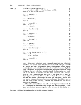
![259
rules in the first conjunct of a body and retracting those rules in the last con-
junct. The programmer must make sure that the rules are retracted in case
the intervening conjuncts fail. Also, the programmer must be careful not to
introduce rules with heads that already exist in the environment; such intro-
duced rules will be added to, not replace, existing rules, and retraction might
accidentally remove more rules than are intended.
2 ◆ GO
..
DEL
Go
..
del, developed by P. M. Hill, is intended to be the successor of Prolog
[Hill 94]. It borrows much of Prolog’s form, but attempts to address many of
the problems and deficiencies of Prolog. It provides modules to make the lan-
guage suitable for large projects, has a strong type system, permits enhanced
logical forms, and has more consistent search-pruning operators. Go
..
del also
directly supports integers, floats, rational numbers, strings, lists, and sets.
2.1 Program Structure
A program in Go
..
del consists of at least one module. Each module is divided
into several parts, most of which are optional.
• module names the module. Modules can also be declared closed (which
means the implementation is not provided, and may well be in a different
language), export (all definitions are exported to other modules), or local
(all definitions are private).
• import lists the modules whose declarations are imported.
• base declares types.
• constructor declares type constructors.
• constant declares constants.
• function lists functions and declares their type. (These are like functors
in Prolog.)
• predicate lists predicates and defines their type.
• delay lists conditions for controlling evaluation of predicates.
• proposition lists propositions.
• Finally, there is a list of rules.
For example, the module in Figure 8.61 calculates factorials.
Figure 8.61 module Factorial. 1
import Integers. 2
predicate Fact : Integer * Integer. 3
Fact(0,1). 4
Fact(1,1). 5
Fact(n,f) <- n > 1 & Fact(n-1,g) & f = g * n. 6
The module is named Factorial and imports types, functions, and predicates
from the (library) module Integers. It has one predicate, Fact, which has
two integer parameters. Three rules define Fact (lines 4–6). The program is
executed by supplying a query, as in Figure 8.62.
Copyright Addison-Wesley. Reproduction fee $.02 per page, per copy.
2 GO
..
DEL](https://image.slidesharecdn.com/advancedprogramminglanguagedesign-230706034617-464d64c2/85/Advanced_programming_language_design-pdf-267-320.jpg)
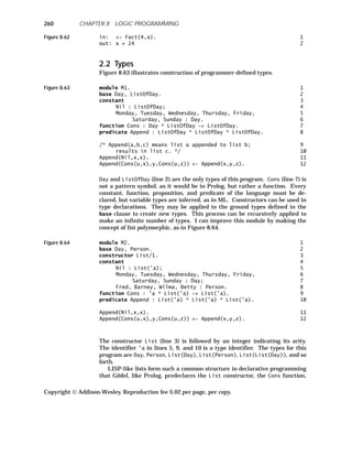
![261
and the Nil constant. The constructors for lists are the same as in Prolog;
the list Cons(Fred,Cons(Bill,x)) can be written as [Fred, Bill | x].
2.3 Logic Programming
Unlike Prolog programs, Go
..
del programs are not limited to Horn clauses.
The following quantifiers and connectives are allowed.
Symbol Meaning
& conjunction (and)
/ disjunction (or)
˜ negation (not)
<- implication
-> right implication
<-> equivalence
all universal quantifier
some existential quantifier
The quantifiers have two parameters, a list of variables and the body, as in
Figure 8.65.
Figure 8.65 module Inclusion. 1
import Lists. 2
predicate IncludedIn : List(a) * List(a) 3
-- IncludedIn(a,b) means list a is included in list b. 4
IncludedIn(x,y) <- all [z] (MemberOf(z,y) <- MemberOf(z,x)). 5
-- MemberOf(a,b) means element a is a member of list b. 6
The rule in line 5 indicates that list x is included in list y if all members of x
are also members of y. This example also illustrates some of the use of mod-
ules. The predicate MemberOf (used in line 5) is declared in the imported
module Lists.
Queries are quite simple to write. For example, assume that a module has
been declared with the classic family relationship predicates and facts Fa-
therOf, MotherOf, ParentOf, AncestorOf, and so forth. Then the query “Does
everyone who has a mother also have a father?” can be written, as in Figure
8.66.
Figure 8.66 <- all [x] 1
(some [z] FatherOf(x,z) <- some [y] MotherOf(x,y))). 2
In practice, some is seldom used, because Go
..
del provides _ as a don’t-care
pattern. The above query can be written more simply as in Figure 8.67.
Copyright Addison-Wesley. Reproduction fee $.02 per page, per copy.
2 GO
..
DEL](https://image.slidesharecdn.com/advancedprogramminglanguagedesign-230706034617-464d64c2/85/Advanced_programming_language_design-pdf-269-320.jpg)
![Figure 8.67 <- all [x] (FatherOf(x,_) <- MotherOf(x,_))
The quantifier some may also be used in queries to restrict the display of re-
sults to the variables of interest to the user. For example, the query in Figure
8.68
Figure 8.68 <- some [y] (ParentOf(x,y) & ParentOf(y,Jane)).
will display the value to which x is bound, but not y. The same query can be
written using the colon notation ( : is read “such that”), as in Figure 8.69.
Figure 8.69 <- x : ParentOf(x,y) & ParentOf(y,Jane).
2.4 Conditionals
Go
..
del allows the use of conditional statements primarily as a concession to
computational efficiency. The structure if condition then formula is logi-
cally equivalent to condition -> formula. The semantics of conditionals dif-
fer procedurally from implications, however. Unlike implications, the
evaluation of a conditional waits until the condition has no free variables.
If the condition and the formula share local variables, the form in Figure
8.70 is used.
Figure 8.70 if some [r1, ..., rn] condition then formula
This form is equivalent to that in Figure 8.71.
Figure 8.71 (some [r1, ..., rn] (condition & formula)) / 1
˜ some [r1, ..., rn] condition. 2
The if construct is defined similarly, but oddly enough, the rule for resolving
the dangling-else problem is contrary to standard convention.
The module for defining LISP-like association lists in Figure 8.72 illus-
trates conditionals.
Figure 8.72 module AssocList. 1
import Strings. 2
base PairType. 3
function Pair : Integer * String -> PairType. 4
predicate Lookup : Integer * String * List(PairType) 5
* List(PairType). 6
Copyright Addison-Wesley. Reproduction fee $.02 per page, per copy.
262 CHAPTER 8 LOGIC PROGRAMMING](https://image.slidesharecdn.com/advancedprogramminglanguagedesign-230706034617-464d64c2/85/Advanced_programming_language_design-pdf-270-320.jpg)
![263
Lookup(key, value, assoc_list, new_assoc_list) <- 7
if some [v] 8
MemberOf(Pair(key,v), assoc_list) 9
then 10
value = v & 11
new_assoc_list = assoc_list 12
else 13
new_assoc_list = [Pair(key,value)| assoc_list]. 14
2.5 Control
Logic programming in its pure form allows the parameters of predicates to be
arbitrarily bound or unbound. As you saw in Prolog, it is often difficult (and
unnecessary) to write rules that cover all cases. Go
..
del uses something like
Prolog’s bound predicate, but it enhances it with a control structure that de-
lays evaluation of predicates until certain conditions are met. Predicates in a
conjunction can be processed like coroutines. For example, the definition of
Permutation in Figure 8.73 might be placed in the Lists module.
Figure 8.73 predicate Permutation : List(a) * List(a). 1
-- Permutation(a,b) means list a is 2
-- a permutation of list b 3
delay Permutation(x,y) until bound(x) / bound(y). 4
Permutation([],[]). 5
Permutation([x| y],[u| v]) <- 6
Delete(u,[x| y],z) & Permutation(z,v). 7
-- Delete(a,b,c) means deleting element a 8
-- from list b gives list c 9
The delay construct in line 4 causes Permutation to pause until one of its pa-
rameters is bound. If it is invoked with both parameters unbound and no
other predicates can be explored to bind one of the parameters, as in Figure
8.74, Permutation will fail. (This behavior is nonmonotonic.)
Figure 8.74 in: <- Permutation(x,y). 1
out: No 2
in: <- Permutation(x,y) & x = [1,2]. 3
out: x = [1,2], y = [1,2]; 4
x = [1,2], y = [2,1] 5
In line 1, neither parameter is bound, so the query fails. In line 3, evaluation
of Permutation delays until the second conjunct is evaluated. That conjunct
binds x to a value, so now Permutation may be invoked.
In order to build a sort program similar to naiveSort in Figure 8.26 (page
243), I will introduce in Figure 8.75 a Sorted predicate for the Lists module.
Copyright Addison-Wesley. Reproduction fee $.02 per page, per copy.
2 GO
..
DEL](https://image.slidesharecdn.com/advancedprogramminglanguagedesign-230706034617-464d64c2/85/Advanced_programming_language_design-pdf-271-320.jpg)
![Figure 8.75 predicate Sorted : List(integer). 1
delay 2
Sorted([]) until true; 3
Sorted([_]) until true; 4
Sorted([x,[y| _]) until bound(x) & bound(y). 5
Sorted([]). 6
Sorted([_]). 7
Sorted([x,y| z]) <- x =< y & Sorted([y| z]). 8
The delay construct in line 2 takes multiple patterns, each of which may be
treated differently. If Sorted is invoked with a list of length 0 or 1, it will not
delay, even if the list element is not bound (lines 3–4). For more complex
lists, Sorted will be delayed until the first two elements of the list are both
bound. I can now use Sorted and Permutation to define a Sort module, as in
Figure 8.76.
Figure 8.76 module Sort. 1
import Lists. -- brings in Sorted and Permutation 2
predicate SlowSort : List(Integer) * List(Integer). 3
SlowSort(x,y) <- Sorted(y) & Permutation(x, y). 4
-- SlowSort(a,b) means list a is sorted to produce b. 5
SlowSort works if either x or y (or both) is bound. If y is bound, Sorted will
not be delayed. If Sorted succeeds, Permutation will either verify that x is a
permutation of y if x is bound or find all values of x that are permutations of
y. If y is not bound and x is, then Sorted(y) will delay, and Permutation will
instantiate y to a permutation of x. The entire permutation need not be pro-
duced before Sorted continues; only the first two elements of the permutation
are necessary. Perhaps these elements are enough to show that y is not
sorted, and this permutation may be abandoned. If the first two elements of y
are in order, Sorted makes a recursive call, which may again be delayed. At
this point, Permutation will continue producing more elements of the permu-
tation. If Sorted fails at any point, Permutation will backtrack to an alterna-
tive permutation. In effect, delay gives Go
..
del lazy evaluation, which makes
SlowSort much faster than Prolog’s equivalent naiveSort in Figure 8.26
(page 243). It is still a very poor sorting method, however.
The delay construct also helps the programmer to guarantee termination.
Consider the definition of Delete in Figure 8.77, which is needed to define
Permutation in Figure 8.73 (page 263).
Figure 8.77 -- Delete(a,b,c) means deleting element a 1
-- from list b gives list c 2
predicate Delete : a * List(a) * List(a). 3
delay Delete(_,y,z) until bound(y) / bound(z). 4
Delete(x,[x| y],y). 5
Delete(x,[y| z],[y| w]) <- Delete(x,z,w). 6
Without the delay in line 4, the query Permutation(x, [1, 2, 3]) would first
Copyright Addison-Wesley. Reproduction fee $.02 per page, per copy.
264 CHAPTER 8 LOGIC PROGRAMMING](https://image.slidesharecdn.com/advancedprogramminglanguagedesign-230706034617-464d64c2/85/Advanced_programming_language_design-pdf-272-320.jpg)
![265
produce the answer x = [1, 2, 3] and then go into an infinite loop. With the
delay present, the six possible permutations are produced, and then Permu-
tation fails.
Go
..
del also allows the programmer to prune the backtrack search tree in a
fashion similar to Prolog’s cut, but in a more consistent fashion. The simplest
version of pruning is bar commit. Bar commit works like conjunction but with
the added meaning that only one solution will be found for the formula in its
scope (to its left); all branches arising from other statements for the same
predicate are pruned. The order of statement evaluation is not specified, so
bar commit lacks the sequential property of cut. For example, a Partition
predicate to be used in Quicksort is shown in Figure 8.78.
Figure 8.78 -- Partition(a,b,c,d) means list a partitioned about 1
-- element b results in lists c and d. 2
predicate Partition : List(Integer) * Integer * 3
List(Integer) * List(Integer) 4
delay 5
Partition([],_,_,_) until true; 6
Partition([u| _],y,_,_) until bound(u) & bound(y). 7
Partition([],y,[],[]) <- bar. 8
Partition([x| xs],y,[x| ls],rs) <- x =< y bar 9
Partition(xs,y,ls,rs). 10
Partition([x| xs],y,ls,[x| rs]) <- x > y bar 11
Partition(xs,y,ls,rs). 12
In this case, I use bar commit (I denote it just by bar in lines 8–11) because
the statements in the definition of Partition (lines 8–12) are mutually exclu-
sive, so it prunes useless computation. It is possible to use bar commit to
prune answers as well.
Go
..
del also provides singleton commit. A formula enclosed in curly brack-
ets { and } will only produce one answer. For example, the query {Permu-
tation([1,2,3], x)} will produce only one of the permutations instead of all
six.
The delay construct can prevent premature bar commits that could lead to
unexpected failures. Figure 8.79 shows how to code the Delete predicate dif-
ferently.
Figure 8.79 -- Delete(a,b,c) means deleting element a 1
1
-- from list b gives list c 2
2
predicate Delete : Integer * List(Integer) * List(Integer). 3
delay Delete(x,[u| _],_) until bound(x) & bound(u). 4
Delete(x,[x| y],y) <- bar . 5
Delete(x,[y| z],[y| w]) <- x ˜= y bar Delete(x,z,w). 6
If the program did not delay Delete until x was bound, the query Delete(x,
[1, 2, 3], y) & x = 2 could commit with x bound to 1, by line 5. Then x = 2
would fail, causing the entire query to fail, because the bar in line 6 prevents
backtracking for another binding to x.
Copyright Addison-Wesley. Reproduction fee $.02 per page, per copy.
2 GO
..
DEL](https://image.slidesharecdn.com/advancedprogramminglanguagedesign-230706034617-464d64c2/85/Advanced_programming_language_design-pdf-273-320.jpg)
![3 ◆ FINAL COMMENTS
In some ways, Prolog is a hybrid of three ideas: LISP data structures, recur-
sive pattern matching as in SNOBOL, and resolution theorem-proving. As a
programming language, Prolog lacks mechanisms for structuring programs
and has no type facilities. It is hard to read Prolog programs, because the or-
der of parameters in predicates is not always obvious. This is a problem in
other languages, but it seems especially severe in Prolog. For all its short-
comings, Prolog is widely used, especially in Europe, for artificial intelligence
rule-based programs. It has been successfully used in such applications as
genetic sequence analysis, circuit design, and stock-market analysis.
Enhancements of Prolog to give it an understanding of constraints and to
organize search differently reduce the difficulty of writing clear and efficient
programs. Various constraint-based extensions to Prolog have been devel-
oped, including CLP(Σ*), which understands regular expressions
[Walinsky 89], and versions that deal with strings in general [Rajasekar 94].
Concurrent logic programming is an active research topic. All the con-
juncts in the body of a rule can be evaluated simultaneously, with bindings of
common variables communicated as they arise between otherwise indepen-
dent evaluators. This technique is called and-parallelism. Similarly, multiple
rules whose heads match a goal can be evaluated simultaneously; this tech-
nique is called or-parallelism. Research topics include the ramifications of
using shared and distributed memory, how to manage bindings for variables,
how much parallelism can be discovered by the compiler in ordinary Prolog
programs, and how the programmer can assist that task in extensions to Pro-
log. One such extension, called Guarded Horn Clauses, allows guard predi-
cates, much like the guards in Ada’s select statement (discussed in Chapter
7), to restrict the rules that are to be considered during concurrent evalua-
tion. Much of the literature on concurrent logic programming has been sur-
veyed by Shapiro [Shapiro 89].
Go
..
del manages to blend Prolog with strong typing, some type polymor-
phism, and modularization, while increasing the range of logical operators. It
also provides lazy evaluation, which makes some naive programs far more ef-
ficient. However, it is a much more complex language; one of Prolog’s advan-
tages is its relative simplicity.
There are other languages specifically intended for knowledge-based rea-
soning. In particular, OPS5 shares with Prolog and Go
..
del the concept of
rules, facts, and queries [Brownston 86]. It is based on an inference engine,
which repeatedly (1) determines which rules match existing facts, (2) selects
one of those rules based on some strategy, and then (3) applies the actions
specified in the selected rule, usually adding to or altering the set of facts.
Step 1 can be extremely costly, but step 3 can propagate changes to a data
structure to make step 1 reasonably efficient.
Copyright Addison-Wesley. Reproduction fee $.02 per page, per copy.
266 CHAPTER 8 LOGIC PROGRAMMING](https://image.slidesharecdn.com/advancedprogramminglanguagedesign-230706034617-464d64c2/85/Advanced_programming_language_design-pdf-274-320.jpg)
![267
EXERCISES
Review Exercises
8.1 Figure 8.10 (page 236) shows the backtrack tree for the query grand-
motherOf(tom,X). Show the backtrack tree with the rules for grand-
motherOf in Figure 8.8 (page 234) reordered as in Figure 8.80.
Figure 8.80 grandmotherOf(X,GM) :- motherOf(X,M) , motherOf(M,GM) . 1
grandmotherOf(X,GM) :- fatherOf(X,F) , motherOf(F,GM) . 2
8.2 It appears that the rules on lines 3 and 4 of Figure 8.23 (page 242) can
be replaced by the single rule append([],X,X). Is this so?
8.3 What is the result of the query in Figure 8.81?
Figure 8.81 in: ?- append([1,2],X,[1,2,3,4]) .
8.4 Modify the eval rules in Figure 8.59 (page 257) so that bodies are inter-
preted from right to left, that is, with the last conjunct first.
8.5 Design a functor fraction with two parameters (the numerator and de-
nominator) and predicate lessThan that takes two fractions and is satis-
fied if the first fraction is less than the second. The lessThan predicate
does not need to be defined for unbound parameters.
Challenge Exercises
8.6 Does Prolog have static or dynamic scope rules for formal parameters?
8.7 Are predicates in Prolog first-, second-, or third-class values? How
about predicate names, functors, and terms?
8.8 Show how to build a stack containing {1,2,3} and to verify that it is a
stack, using the definitions of Figure 8.20 (page 240).
8.9 In Figure 8.20 (page 240), I defined nonhomogeneous stacks. Show how
the existence of a built-in integer predicate allows you to define integer
stacks.
8.10 In Figure 8.20 (page 240), pop is a predicate name. Rewrite this exam-
ple so that pop is a functor.
8.11 In Figure 8.26 (page 243), how many solutions are there to naive-
Sort([11,2,11],S)?
8.12 In Figure 8.26 (page 243), how many solutions are there to
naiveSort(S,[1,2])?
8.13 As an alternative to naiveSort and bubbleSort, encode insertionSort
in Prolog. Make sure your program works correctly in all four cases of
insertionSort(α,β), whether α or β is a constant or a variable.
Copyright Addison-Wesley. Reproduction fee $.02 per page, per copy.
EXERCISES](https://image.slidesharecdn.com/advancedprogramminglanguagedesign-230706034617-464d64c2/85/Advanced_programming_language_design-pdf-275-320.jpg)
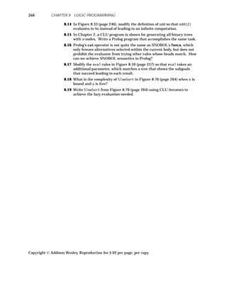
![Figure 9.1 StringVar := "this is a very long string that c 1
I place on several lines, but it represents c 2
a string without line breaks or gaps." 3
Operations on strings are provided either by predefined procedures or by
operators in the language. The simplest operations on strings, such as copy-
ing, equality testing, and lexical comparison, are often provided as overloaded
meanings of := , = , and < . Another simple operation is concatenation, of-
ten represented by the overloaded operator + . (SNOBOL represents con-
catenation by an empty space operator, which is quite confusing, particularly
since the same invisible operator also represents pattern matching!) In addi-
tion, a few languages, such as ABC, provide operators for string repetition
("ho" * 3 is "hohoho"), string length, and arcane operations such as finding
the minimum character in a string.
Languages usually provide ways to convert other data types to strings.
This facility is particularly important for output, which is often a long string
computed from values of various types. Conversions to string are usually
separate functions for each type to be converted, but C has a single function
sprintf that can convert and concatenate any combination of basic types ac-
cording to a format string, as in Figure 9.2.
Figure 9.2 IntVar := 23; 1
sprintf(ResultString, 2
"Give me %d number%s between %5g and 10%c.", 3
IntVar, if IntVar = 1 then "" else "s" end, 4
4.5, ’0’"); 5
The format string in line 3 is copied to ResultString, but certain escapes pre-
fixed by % cause later actual parameters to be converted and inserted into
the string. The formats are specified by %d for integer, %s for string, %g for
float, and %c for character. Formats can include width specifiers, as shown by
%5g. This code places in ResultString the value
"Give me 23 numbers between 4.5 and 100."
A related and even simpler method is provided by Sal in the form of
edited strings [Sturgill 89]. Figure 9.3 is the edited string equivalent of Fig-
ure 9.2.
Figure 9.3 IntVar := 23; 1
ResultString := 2
’Give me {IntVar} numberc 3
{if IntVar = 1 then "" else "s" end} c 4
between {4.5:5} and 10{’0’}.’ 5
Expressions in braces are evaluated at runtime and formatted as appropriate
to their type and according to any width specification given. Edited strings
use a different set of delimiters from ordinary strings as a way to warn the
compiler to inspect them for included expressions, which the compiler inter-
prets to generate code. This code is executed when the edited string is first
Copyright Addison-Wesley. Reproduction fee $.02 per page, per copy.
270 CHAPTER 9 AGGREGATES](https://image.slidesharecdn.com/advancedprogramminglanguagedesign-230706034617-464d64c2/85/Advanced_programming_language_design-pdf-278-320.jpg)
![271
evaluated; the result is an ordinary string that is not reevaluated later.
Edited strings are more type-secure than the sprintf function, because there
is no way to accidentally request that a value of some type be treated as a dif-
ferent type.
Languages often provide either a special syntax or a function call to ex-
tract substrings of a subject string based on position and length, as in Figure
9.4.
Figure 9.4 substr("A sample", 3, 4)
This string evaluates to "samp", starting at the third position of "A sample"
and continuing for 4 characters.
It is also common to provide for character or substring search. Search can
be designed to return a Boolean to indicate success, the position of the char-
acter or substring if found (0 otherwise), or a pointer to the character or sub-
string if found (nil otherwise), as in Figure 9.5.
Figure 9.5 CharSearch("sample string", ’s’) 1
StringSearch("Target string", "get") 2
The search in line 1 could return true, 1, or a pointer to the entire string.
The search in line 2 could return true, 4, or a pointer to the substring "get
string". There might also be variants to conduct the search from right to
left.
Slightly more complex than searching for characters is extracting data
from a string while converting types; see Figure 9.6.
Figure 9.6 MyString := "4 and 4 make 8 in base 10" 1
sscanf(MyString, "%d and %d make %g.", First, Second, 2
Third); -- First := 4, Second := 4, Third := 8.0 3
Here the formats are used not to convert from numeric data to string data,
but the reverse, to convert parts of the string into numeric data. The occur-
rences of %d in line 2 cause the substring "4" to be converted to the integer 4;
the %g format converts "8" to the real 8.0.
Another way to extract data from a string is to split it into fields based on
some character. Several languages (for example, ABC, Perl, and Sal) provide
a split procedure that takes a string and a set of characters considered to be
field separators and a string array (passed by result) into which the given
string is to be separated, as in Figure 9.7.
Figure 9.7 split("Veni, vidi, vici", ",", ResultArray)
This call would assign "Veni" into ResultArray[0], " vidi" into Result-
Array[1] (with the initial space), and " vici" into ResultArray[2].
Copyright Addison-Wesley. Reproduction fee $.02 per page, per copy.
1 STRINGS](https://image.slidesharecdn.com/advancedprogramminglanguagedesign-230706034617-464d64c2/85/Advanced_programming_language_design-pdf-279-320.jpg)
![1.2 Representation
Usually, programmers don’t need to worry about how a language implementa-
tion represents strings. However, the representation can affect both the
speed of computation and the way the program must manipulate strings. For
example, C defines strings as consecutive characters terminated by a null (bi-
nary zero) character. This representation makes it slow to concatenate a
string to the end of another (the implementation must find the end of the sec-
ond string by a linear method) and does not allow nulls to be contained within
strings. It encourages a programming style in which a variable points into
the string and advances character by character until the terminating null is
seen.
Alternative representations have some advantages. If the length of the
string is encoded, perhaps in the first few bytes, then concatenation becomes
faster, and strings may contain null characters. If strings are declared with a
compile-time length, many operations become faster, and the compiler can
keep track of the length of intermediate strings in complex expressions.
However, some operations produce results whose length cannot be predicted.
For example, a substring operation might take a variable length parameter.
Therefore, languages in which strings are explicitly declared usually declare
the maximum length that the string value might attain. This information de-
termines storage requirements but does not dictate the length of particular
values put into storage.
One attractive proposal is to omit a string-length code at the start of the
storage area for a string, use a terminating null, but use the last byte of the
storage area to indicate the distance back to the terminating null [Bron 89].
If the string just fits in the storage area, so that the terminating null is in the
last place, the null looks like the number 0, indicating zero distance to the
terminating null. This representation makes it a bit harder for programs to
build new strings directly, but a reasonable library of string-building opera-
tions can circumvent this problem, and programs may still scan through
strings by using explicit pointers.
1.3 Pattern Matching
Sal, Awk, and Perl provide a match operator ˜ that compares a target string
to a regular expression. The result is Boolean, indicating success. A regular
expression is a string, where most characters match themselves, but some
characters and character combinations have special meanings. The following
table lists some of these special meanings; Perl has an even richer set.
Copyright Addison-Wesley. Reproduction fee $.02 per page, per copy.
272 CHAPTER 9 AGGREGATES](https://image.slidesharecdn.com/advancedprogramminglanguagedesign-230706034617-464d64c2/85/Advanced_programming_language_design-pdf-280-320.jpg)
![273
Regular expression Matches
. any character
< start of word
> end of word
s white space
d a digit (like [0-9])
w a word
ˆ the beginning of the target string
$ the end of the target string
[abc...] any character in the set; ranges like: [3-7A-P]
[ˆabc...] any character not in the set
r1 | r2 either r1 or r2 (alternation)
r* zero or more r’s
r+ one or more r’s
r? zero or one r’s
r{3,5} match 3, 4, or 5 r’s
(r) match r, call it a group
2 string matched by the second group
Some of these expressions, like . and ‘s , match (and “use up”) a single
character. Others, like < and ˆ , do not use up any characters. For exam-
ple, the < expression matches the beginning of an alphanumeric region of
the string; it is used to signal the start of a word. Grouping a subpattern al-
lows you to refer to it later. Groups are numbered according to the left-to-
right order of their opening parentheses. Figure 9.8 shows some examples of
regular expressions.
Figure 9.8 "literal" -- matches "literal" 1
"l*iteral" -- matches "iteral", "literal", "lllliteral" ... 2
"(l | b)(i| o)b2" -- matches "libi", "lobo", "bibi", "bobo" 3
"[lb][io]b" -- matches "lib", "lob", "bib", "bob" 4
The match operator can return the start and length of the matched substring
via predeclared global variables or make them available through functions to
be called after the match. If several matches are possible, one match is cho-
sen. The usual rule is that * extends its match as far as possible and that
the alternatives indicated by | are tried in the order given. In Perl, the
search can be made insensitive to the case of the subject string, it can be
made to start either at the beginning of the string or where the previous
search left off, and it can be set not to extend the match as far as possible.
Slightly more sophisticated than matching a pattern is replacing the
matched substring with new contents. The new contents can depend on parts
of the matched patterns. Those parts are typically parenthesized groups,
numbered in the order of their opening parentheses, as in Figure 9.9.
Figure 9.9 MyString := "here is a nice sample"; 1
Substitute(MyString, "(i(s) )", "wa2"); 2
The Substitute procedure in line 2 assigns "here was a nice sample" to My-
Copyright Addison-Wesley. Reproduction fee $.02 per page, per copy.
1 STRINGS](https://image.slidesharecdn.com/advancedprogramminglanguagedesign-230706034617-464d64c2/85/Advanced_programming_language_design-pdf-281-320.jpg)
![String. The ‘2’ in line 2 fills in what the second group, (s), matched,
namely, "s". Some languages provide sequences that can be placed in the
third parameter of Substitute to indicate the part of the target string before
the match, the entire matched part, and the part after the match, as in Fig-
ure 9.10.
Figure 9.10 MyString := "I think, therefore I am"; 1
Substitute(MyString, ",", " that ‘&’,"); 2
The expression ‘&’ in line 2 indicates the entire string, built up of the
parts before, during, and after the match. The substitution changes MyString
to "I think that I think, therefore I am, therefore I am".
1.4 Associative Arrays
Languages dealing with strings often provide a data type known as an asso-
ciative array, which is indexed by strings instead of by integers or other
scalar types. Associative arrays are usually implemented by hash tables. In
some languages, like Sal and SNOBOL, the declaration of such an array indi-
cates how large to make the hash table. If more elements are stored than the
hash table size, access will become progressively slower but will still work.
Other languages, like Perl, use extensible hashing and do not require any size
declaration. ABC uses binary trees instead of hashing, so that a program can
iterate through the array in key order. Other languages can only iterate in
an implementation-dependent order.
Associative arrays are quite helpful in database applications. For exam-
ple, to check for duplicates in a database with one field, say, StudentName, I
could use the Boolean associative array Present of Figure 9.11.
Figure 9.11 variable 1
Present : array string of Boolean; 2
ThisEntry : string; 3
loop 4
ThisEntry := GetNextEntryOfDatabase(); 5
if ThisEntry = "" then break end; -- exit loop 6
if defined Present[ThisEntry] then -- found duplicate 7
write("{ThisEntry} is a duplicate."); 8
end; 9
Present[ThisEntry] := true; 10
end; 11
In line 7, the defined operator indicates whether a value has been defined for
the particular index value given; it returns a Boolean. The assignment in
line 10 could just as easily use false; what counts is that some value is
placed in Present[ThisEntry].
Associative arrays often come with a control structure for iterating over
all index values that have been defined. Figure 9.12 continues the previous
example.
Copyright Addison-Wesley. Reproduction fee $.02 per page, per copy.
274 CHAPTER 9 AGGREGATES](https://image.slidesharecdn.com/advancedprogramminglanguagedesign-230706034617-464d64c2/85/Advanced_programming_language_design-pdf-282-320.jpg)
![275
Figure 9.12 for Entry in Present do 1
write(Entry); 2
end; 3
1.5 Substrings as First-Class Values
Allowing substrings to be first-class values of a predeclared substring type
has several advantages [Hansen 92]. Substring values can record not only
their contents but also the identity of their base string. Dynamic allocation of
space for substrings can be handled by the language at runtime.
Each value of the substring type contains a base string (perhaps imple-
mented as a pointer) and the left and right positions in that string that de-
limit the substring. As with Icon, I understand positions to be between
characters of the string.
The primitive operations on substrings can be simple and few. Here is a
reasonable set of primitive operations:
• start(x). Returns a substring with the same base as x, with both left
and right set to left of x.
• base(x). Returns a substring with the same base as x, left set before the
first character of x, and right set to after the last character of x.
• next(x). Returns a substring with the same base as x, left set to right of
x, and right set one character after left if possible. Otherwise, right is set
to the same position as left.
• prev(x). Returns a substring with the same base as x, right set to left of
x, and left set one character before right if possible. Otherwise, left is set
to the same position as right.
• extent(x,y). If x and y have different base strings, returns an empty
substring of the empty base "". Otherwise, returns a substring with right
set to the right of y and left set to either left of x or right of y, whichever is
earlier in the base.
• x = y. The base strings of the two substrings are compared character by
character between their left and right positions. The result is true if and
only if the lengths are identical and the selected characters match exactly.
• x + y. Returns a substring containing a new base string that is the con-
catenation of the substrings x and y, and left and right at the beginning
and end of that new base string.
• x := y. The old value of x is discarded; x acquires the same value as y,
including the base string and the left and right positions.
Given these primitive operations, I can write a function that takes a sub-
string representing a word terminated by blanks and returns a substring rep-
resenting the next word, as in Figure 9.13 [Hansen 92].
Copyright Addison-Wesley. Reproduction fee $.02 per page, per copy.
1 STRINGS](https://image.slidesharecdn.com/advancedprogramminglanguagedesign-230706034617-464d64c2/85/Advanced_programming_language_design-pdf-283-320.jpg)
![Figure 9.13 function NextWord(value aWord : substring) : substring; 1
begin 2
loop -- skip to end of word 3
aWord := next(aWord); 4
if aWord ≠ " " then break end; 5
end; 6
while next(aWord) ≠ "" and next(aWord) ≠ " " do 7
aWord := extent(aWord, next(aWord)); 8
end; 9
return aWord; 10
end; -- NextWord 11
The primitive substring operations can be used to build slightly more
sophisticated operations, such as rest, which returns all but the first charac-
ter of its substring parameter, and last, which returns just the last character
of its substring parameter. They can also be used to build Icon’s matching
procedures.
1.6 SNOBOL
SNOBOL was developed by Ralph E. Griswold and others at Bell Telephone
Laboratories around 1965 [Griswold 71]. It has a strange syntax, partially
because it was developed before Algol-like syntax became popular. Spaces act
as both the concatenation and the match operators. The only statement form
includes pattern match, replacement, and success and failure gotos. To avoid
confusion, I translate all the SNOBOL examples into an Ada-like syntax, us-
ing match and replace operators. SNOBOL uses dynamic typing and dy-
namic scope rules; its primitive data types are strings, integers, and reals.
The structured types include patterns (distinct from strings), nonhomoge-
neous arrays, and associative arrays.
Variables are not declared; all conceivable strings (even the empty string)
name variables. Initially, all variables have the value "". In a sense, there-
fore, all string values point to other strings, as in Figure 9.14.
Figure 9.14 somewhere := "over"; 1
over := "the"; 2
the := "rainbow"; 3
write(somewhereˆˆ); -- writes "rainbow" 4
SNOBOL is homoiconic, after a fashion. A program is a string, and it is
possible at runtime to compile a string and to branch to a label in it. How-
ever, this facility is much less attractive than LISP’s equal treatment of pro-
gram and data structure. SNOBOL has not been heavily used for artificial
intelligence programming.
SNOBOL patterns are like regular expressions, but more powerful. They
are structured values built recursively. The simplest patterns are string liter-
als and string-valued expressions, which match themselves. More complex
patterns are formed by sequencing (somewhat like and), alternation (some-
what like or), and by invoking pattern-returning predeclared functions. Pat-
terns are matched by a backtracking algorithm, trying earlier alternatives
first. Backtracking in pattern matching is very similar to backtracking in
Copyright Addison-Wesley. Reproduction fee $.02 per page, per copy.
276 CHAPTER 9 AGGREGATES](https://image.slidesharecdn.com/advancedprogramminglanguagedesign-230706034617-464d64c2/85/Advanced_programming_language_design-pdf-284-320.jpg)
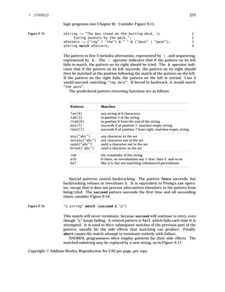
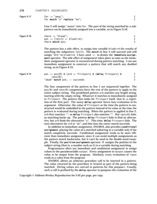
![279
actual parameters and the invocation of the procedure until match time. If
the procedure fails, then that part of the pattern match fails, and backtrack-
ing takes over. Information resulting from the match so far can be passed to
the procedure via immediate assignment to global variables or to local vari-
ables passed as actual parameters.
1.7 Icon
Icon was developed by Ralph E. Griswold, one of the developers of SNOBOL,
in the late 1970s as a result of his dissatisfaction with how SNOBOL’s pat-
terns fit into the language [Griswold 80]. It retains the virtues of SNOBOL’s
pattern matching without a pattern data type. It is an expression-oriented
language, with each evaluation resulting in either a value (counted as a suc-
cess) or failure. Instead of using Boolean values, conditionals base their ac-
tions on the success or failure of evaluating their conditions.
The first novel idea in Icon is the scan statement. (I call it a statement,
even though all constructs in Icon are actually expressions, because it is usu-
ally not used for its value.) This statement introduces a name scope that cre-
ates a new binding for two predeclared variables, subject and pos, which
specify the current string being matched and the current position within the
string. Consider Figure 9.20 (I take liberties with actual Icon syntax to keep
my examples consistent).
Figure 9.20 scan "peristalsis" using 1
write("[" + move(4) + "]") 2
end; 3
This program prints "[peri]". The scan in line 1 maps subject to "peri-
stalsis" and sets pos initially to 1. The body of scan is in line 2; it implicitly
uses both subject and pos (modifying the latter). The predeclared procedure
move causes the position to be incremented, if subject is long enough, and if
it succeeds, it returns the substring of subject over which it has advanced.
The + operator is string concatenation. After the body, both subject and pos
revert to whatever values they had before. Figure 9.21 shows a more complex
nested example.
Figure 9.21 scan MyString using 1
loop -- each iteration deals with one word 2
scan tab(upto(" ")) using 3
if upto("-") then -- word has a hyphen 4
write(subject); 5
end; 6
end; -- scan tab(upto(" ")) 7
move(1); -- past " " 8
end; -- loop 9
end; -- scan MyString 10
This program prints out all space-delimited words in MyString that contain a
hyphen. The outer scan (lines 1–10) contains a loop that repeatedly advances
pos to a space, scans the intervening word (lines 3–7), and then moves past
the space (line 8). The predefined function upto (lines 3 and 4) returns the
Copyright Addison-Wesley. Reproduction fee $.02 per page, per copy.
1 STRINGS](https://image.slidesharecdn.com/advancedprogramminglanguagedesign-230706034617-464d64c2/85/Advanced_programming_language_design-pdf-287-320.jpg)
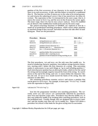
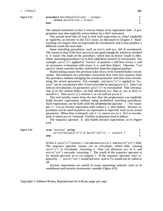
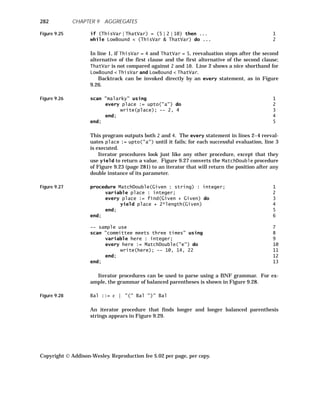
![283
Figure 9.29 procedure Bal() : integer; 1
every 2
match("") | ( 3
tab(match("(")) & tab(Bal()) & 4
tab(match(")")) & tab(Bal()) 5
) 6
do 7
yield pos; 8
end; 9
end; 10
-- sample use 11
scan "()(())(" using 12
variable here : integer; 13
every here := Bal() do 14
write(here); -- 1, 3, 7 15
end; 16
end; 17
1.8 Homoiconic Use of Strings: Tcl
Several syntax rules in Tcl interact to make it homoiconic. Lists are repre-
sented as strings; the individual elements are delimited by white space. Ev-
ery string names a variable. The R-value of a variable is denoted by $ before
the string that represents the variable. (This rule makes Tcl programs error-
prone, because it is so easy to forget the $ .) Strings need not be delimited by
quotes unless they have embedded spaces. There are quotes ( { and } ) that
prevent any evaluation within a string, quotes ( " ) that allow evaluation, and
quotes ( [ and ] ) that force the string to be evaluated. Evaluating a string
means treating it as a series of commands delimited by end-of-line characters
or semicolons. Each command is the name of a procedure (many are prede-
clared; I will show them in bold monospace) followed by parameters. The
whole program is a string to be evaluated. Figure 9.30 shows a simple Tcl ex-
ample.
Figure 9.30 set a 4 -- a := 4 1
set b [expr $a + 5] -- b := 9 2
while {$b > 0} { 3
puts "b is now $b" 4
set b [expr $b - 2] 5
} 6
This program prints b is now 9 and then four more similar outputs. Line 1
is the assignment statement. It takes the name, not the R-value, of the vari-
able to be assigned. Line 2 shows the quotes that force evaluation: [ and ] .
The expr command evaluates any number of parameters as an arithmetic ex-
pression. It returns the value of that expression. Line 3 introduces the
quotes that prevent evaluation: { and } . The while command takes two
unevaluated strings, the first representing a conditional and the second rep-
resenting the body of the loop. It repeatedly invokes expr on the first param-
eter, and if the result is true, it evaluates the second parameter, thereby
Copyright Addison-Wesley. Reproduction fee $.02 per page, per copy.
1 STRINGS](https://image.slidesharecdn.com/advancedprogramminglanguagedesign-230706034617-464d64c2/85/Advanced_programming_language_design-pdf-291-320.jpg)
![executing the body. The body contains end-of-line characters, allowing the
parser to separate it into individual statements. Line 4 shows the last kind of
quotes, which can build a string containing spaces, but which do not prevent
evaluation of such constructs as $b.
To see how Tcl is homoiconic, consider Figure 9.31, a less readable version
of the same program.
Figure 9.31 set a 4 -- a := 4 1
set rhs {expr $a +} -- rhs := "expr $a +" 2
set rhs [append rhs 5] -- rhs := "expr $a + 5" 3
set b [eval $rhs] -- b := 9 4
set cond {$b > 0} -- cond := "$b > 0" 5
set body { 6
puts "b is now $b" 7
set b [expr $b - 2] 8
} 9
while $cond $body 10
The condition and the body of the while loop in line 10 are the result of previ-
ous computations. Even commands can be computed, as in Figure 9.32.
Figure 9.32 set a ile -- a := "ile" 1
wh$a {$b > 0} {set b [expr $b - 2]} 2
Line 2 is actually a while command, because the first word evaluates to
while.
2 ◆ ARRAYS: APL
Arrays are especially important in mathematical computation. One of the
principal advances in FORTRAN 90 over earlier versions of FORTRAN is its
ability to manipulate arrays without dealing with the individual array ele-
ments. However, the best example of an array language is not FORTRAN,
but APL. The APL language was invented by Kenneth E. Iverson in the early
1960s and has had a small but devoted following ever since. It could be con-
sidered a single-minded language: All computation is cast in the mold of ar-
ray manipulation. Its practitioners point with pride at the conciseness of
their programs; detractors point with scorn at the unreadability of the same
programs. APL has long suffered from the fact that most of its operators are
not normal ASCII symbols, so ordinary keyboards are not adequate for repre-
senting APL programs. Dialects such as J and APL/11 use several ASCII
characters together to represent the unusual symbols. My examples expand
unusual symbols into keywords to help you read them.
APL programs must be studied; they cannot simply be read. Not only does
APL have an unusual character set, but it lacks control structures such as
while and conditionals.
APL’s greatest strength is its ability to handle arrays of any dimension
with the same operators that apply to scalars (which are zero-dimensional ar-
rays). The meaning is to apply the operator pointwise to each member of the
array. The resulting uniformity, along with the wealth of arithmetic opera-
Copyright Addison-Wesley. Reproduction fee $.02 per page, per copy.
284 CHAPTER 9 AGGREGATES](https://image.slidesharecdn.com/advancedprogramminglanguagedesign-230706034617-464d64c2/85/Advanced_programming_language_design-pdf-292-320.jpg)
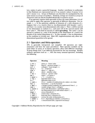
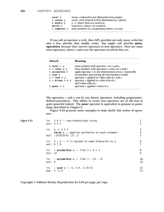
![287
in: max accumulate a 14
out: 5 15
in: * accumulate recip a -- .333333333 * .25 * .2 16
out: .0166666667 17
in: a=a -- pointwise comparison 18
out: 1 1 1 19
in: ≠ accumulate a=a -- determine parity 20
out: 1 21
in: fill 4 22
out: 1 2 3 4 23
in: recip fill 4 24
out: 1 .5 .333333333 .25 25
in: (2 3) layout fill 6 26
out: 1 2 3 27
4 5 6 28
in: a := (2 3) layout fill 6 29
a[1,1] := 9 -- indices start at 1 30
a[2,] := 8 -- entire row; 8 is spread 31
a[,2] := 7 -- entire column; 7 is spread 32
a 33
out: 9 7 3 34
8 7 8 35
in: (2 3) layout (5 6) -- last parens not needed 36
out: 5 6 5 37
6 5 6 38
in: + accumulate (2 3) layout (5 6) 39
out: 16 17 40
in: + scan (2 3) layout (5 6) 41
out: 5 11 16 42
6 11 17 43
in: 1 rotate (3 2) layout fill 6 44
out: 3 4 45
5 6 46
1 2 47
in: (fill 4) + inner * (fill 4) 48
-- sum of products; last parens not needed 49
out: 30 50
in: (fill 2) + inner * ((2 3) layout fill 6) 51
-- sum of products 52
out: 9 12 15 53
Copyright Addison-Wesley. Reproduction fee $.02 per page, per copy.
2 ARRAYS: APL](https://image.slidesharecdn.com/advancedprogramminglanguagedesign-230706034617-464d64c2/85/Advanced_programming_language_design-pdf-295-320.jpg)
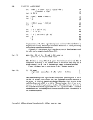
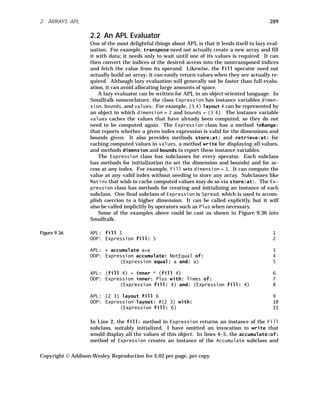
![gives it both an operator, represented as the class NotEqual, and an expres-
sion to manipulate (all of line 5). If it needs to make calculations, it can in-
stantiate NotEqual as many times as needed and initialize those instances to
the appropriate values. Array literals such as #(2 3) (line 10) could be co-
erced to the appropriate constant Expression, or I could require that they be
explicitly converted by saying Expression constant: #(2 3).
2.3 Incremental Evaluation
In some applications, the same program is executed repeatedly on slightly dif-
ferent inputs. For example, spreadsheet programs are often reevaluated with
slightly different data. Functional programming languages have been de-
signed that can quickly evaluate expressions given new data expressed as a
modification of previous data [Yellin 91].
I want to show you how this idea can be embedded in an APL interpreter.
To keep the discussion simple, I do not use a lazy interpreter, and I assume
that the program is a single function with no internal variables. Given an old
value and a new value, a delta represents how to change the old value to the
new value. Of course, by value I mean an array of some shape. The delta and
the old value together are enough to completely specify the new value.
Every operator instance records the most recent value it has produced. It
provides that value to its caller as a delta. The ultimate caller is typically the
outer-level write routine, which uses the delta it receives to display the value
of the program. (It might even display the delta, if the user is interested in
that representation instead of the fully expanded result.) The first time the
program is run, the deltas show the difference between the void value (not
even a zero-dimensional array!) and the initial value.
In order for this scheme to be efficient, incremental computation should
usually not be more expensive than computing from scratch. If we are lucky,
incremental computation is very inexpensive. An occasional inefficient re-
computation is perfectly acceptable, though.
Achieving efficiency has two parts. First, the format for the deltas should
not be longer than the new value. If a value has changed in major ways, it is
better just to provide the new value outright. For APL arrays, a delta might
indicate dimensions to delete, indices within a dimension to delete, particular
values to change, and new indices within a dimension to add (with their val-
ues). For example, the delta from 1 3 4 5 7 to 1 2 4 5 might be represented as
“change at index 2 to value 2, delete index 5.”
Second, each operator and meta-operator should be implemented to take
advantage of deltas. For example, the + operator generates an output delta
that only includes indices where the input deltas indicate a change. The ac-
cumulate meta-operator could make use of an inverse to the operator it is
given, if one exists, in order to remove the effects of any deleted array ele-
ments before adding the effects of inserted elements.
Copyright Addison-Wesley. Reproduction fee $.02 per page, per copy.
290 CHAPTER 9 AGGREGATES](https://image.slidesharecdn.com/advancedprogramminglanguagedesign-230706034617-464d64c2/85/Advanced_programming_language_design-pdf-298-320.jpg)
![291
3 ◆ DATABASE LANGUAGES
Databases are much more varied in structure than strings or arrays. The
range of languages designed for databases is also quite wide. Database lan-
guages tend to look like ordinary algebraic languages and are often Algol-
based. They integrate database operations by providing additional data types
and control constructs. Typically, programmers need to keep two “current lo-
cations” in mind: the current point of execution of the program, and the cur-
rent record of a database. In some languages, it is also necessary to keep the
current relation in mind.
3.1 Data Types
There are several ways to represent data in a database, known as hierarchi-
cal, network, and relational. I concentrate on relational databases, in which
information is stored in relations, which are persistent homogeneous arrays
of records.
My examples are taken from dBASE [Simpson 87], Sal [Sturgill 89], and a
higher-level language, SQL. My examples will be based on the relations
shown in Figure 9.37.
Figure 9.37 People : relation 1
FirstName, LastName : string; 2
BirthYear : integer; 3
end; 4
Events : relation 5
Place, What : string; 6
EventYear : integer; 7
end; 8
That is, People and Events are homogeneous persistent arrays of records
with the fields as shown. I have not limited the length of the string fields
(dBASE requires declaring the exact length; Sal does not, but does allow pat-
terns that restrict valid values) nor the range of the integer fields (dBASE re-
quires specifying the number of characters in a string version of the field; Sal
allows explicit range specification). The data specifications, known as
schemata, are usually stored in files, as are the relations themselves.
Schemata are built either interactively (dBASE) or by a specification file
(Sal).
In dBASE, a program that uses a relation opens it for use, at which time
the field names become defined. dBASE is dynamic-typed. Runtime func-
tions are available to determine the types of fields. In Sal, a program must
read the relation into a local relation variable before using it and must specify
which fields are to be read. Runtime type checking verifies that the specified
fields actually exist and are consistent with the uses to which they are put.
Both dBASE and Sal allow the programmer to restrict attention to those
records in a relation for which some Boolean expression holds. In dBASE,
there are two techniques for restriction. First, a filter statement causes
records to be invisible, as in Figure 9.38.
Copyright Addison-Wesley. Reproduction fee $.02 per page, per copy.
3 DATABASE LANGUAGES](https://image.slidesharecdn.com/advancedprogramminglanguagedesign-230706034617-464d64c2/85/Advanced_programming_language_design-pdf-299-320.jpg)
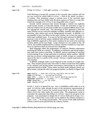
![293
Some database languages, such as DMAWK [Sicheram 91], permit a field
to have multiple values within a single record. Each field is an implicit zero-
based array; the programmer can refer to FirstName[2], for example, to get a
person’s third name. DMAWK has the strange rule that omitting the sub-
script represents the last element of the array for R-values, but one past the
end for L-values. Assigning a nil value to a field deletes the field. Therefore,
in a record that is initially empty, Figure 9.40
Figure 9.40 FirstName := "Jones"; -- FirstName[0] := "Jones" 1
FirstName := FirstName; -- FirstName[1] := FirstName[0] 2
FirstName[1] := nil; -- delete FirstName[1] 3
FirstName := "Hamzah"; -- FirstName[1] := "Hamzah" 4
would have the effect of setting FirstName[0] and FirstName[1] both to
"Jones" (lines 1 and 2) before clearing the latter (line 3), later resetting the
latter to "Hamzah" (line 4).
Since database languages deal heavily with string data, they can take ad-
vantage of the data structures and string operations discussed earlier in this
chapter, particularly associative arrays and pattern matching. Sal, for exam-
ple, has both.
3.2 Control Structures
Control structures are needed for setting the current-record mark and for it-
erating through all relevant records in a relation. Sal has no methods for ex-
plicitly moving the current-record mark; it only provides for iteration.
In dBASE, seek uses the current order to search quickly for a record
whose order value matches the given expression. In addition, the program-
mer can undertake a search within a subset of the records for one whose
fields match any Boolean expression. Such a search is slower than seek, be-
cause the order information allows an O(log n) binary search, where n is the
number of records. Finally, dBASE provides a goto statement that sets the
current-record mark to any given record by serial number in the natural or-
der, and a skip statement that moves any number of records relative to the
current record in the current order. There are predeclared routines that indi-
cate the value of the current-record mark and the number of records in the
relation.
Iteration is accomplished in Sal by a foreach statement. In Sal, foreach
indicates which relation variable to use and names a control variable, as in
Figure 9.41.
Figure 9.41 variable 1
People : relation 2
FirstName, LastName : string; 3
BirthYear : integer; 4
end; 5
Person : tuple of People; 6
Copyright Addison-Wesley. Reproduction fee $.02 per page, per copy.
3 DATABASE LANGUAGES](https://image.slidesharecdn.com/advancedprogramminglanguagedesign-230706034617-464d64c2/85/Advanced_programming_language_design-pdf-301-320.jpg)
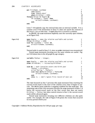
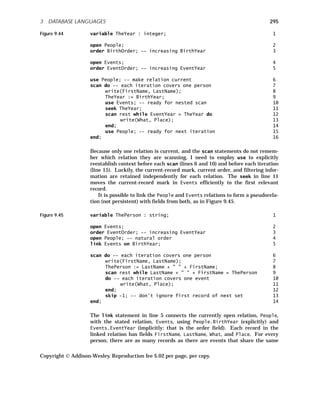
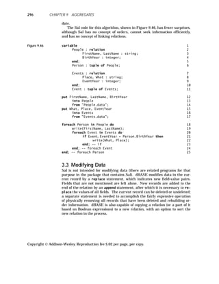
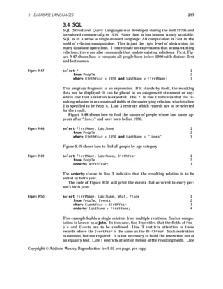
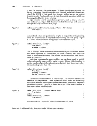
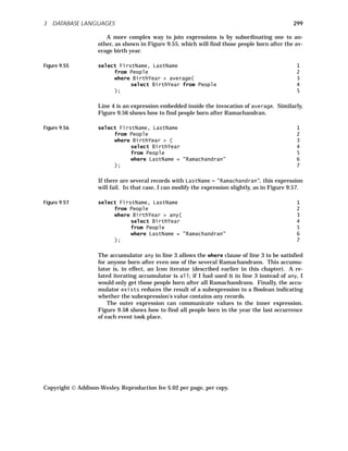
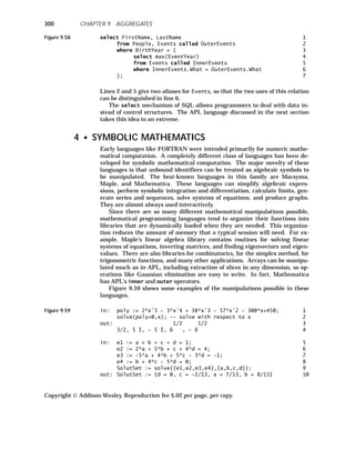
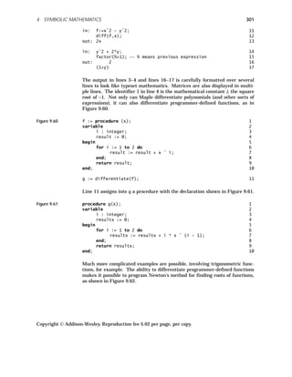
; 1
begin 2
Fibonacci(n-1) + Fibonacci(n-2); 3
end; 4
Fibonacci(0) := 0; -- assigns to the remember table 5
Fibonacci(1) := 1; -- assigns to the remember table 6
The option remember in line 1 causes Fibonacci to store and use previously
computed values. The assignments in lines 5 and 6 explicitly place values in
Fibonacci’s remember table, making it unnecessary to put special cases in
the body of the procedure itself.
5 ◆ FINAL COMMENTS
Languages that are aimed at special applications tend to concentrate on par-
ticular aggregates in order to help the programmer write clear and efficient
code. SNOBOL and Icon are particularly designed for applications that need
to read and manipulate textual data. The related scripting languages are
used to scan text files, extract information, print reports, construct input for
other programs, and collect output from other programs. Such languages in-
clude command interpreters like Csh, stream editors like Awk and Sed, and
interpreted languages such as Perl and Tcl. These languages generally have
many features for manipulating strings. Extensions to Prolog (see Chapter 8)
for dealing with strings are actively being researched, giving rise to lan-
guages such as CLP(Σ). The problem that string Prolog must grapple with is
Copyright Addison-Wesley. Reproduction fee $.02 per page, per copy.
302 CHAPTER 9 AGGREGATES](https://image.slidesharecdn.com/advancedprogramminglanguagedesign-230706034617-464d64c2/85/Advanced_programming_language_design-pdf-310-320.jpg)
![303
that unification over strings is intractable (it is at least NP hard, although it
is decidable) [Rajasekar 94]. Which language to use depends, of course, on
what is available (Csh is only available under Unix), how fast the program
must run (interpreted programs are generally slower), and how sophisticated
the string manipulations need to be.
SNOBOL has some excellent points. The fact that backtracking is built
into the language frees the SNOBOL programmer from writing backtrack
code, which is tricky to get right. Patterns free the programmer from worry-
ing about maintaining an explicit variable for the focus of attention (the posi-
tion in the subject string that is being matched). Patterns can be assigned to
variables and used to build more complex patterns. In fact, the BNF for a
context-free (and even a context-sensitive) language can be represented di-
rectly in SNOBOL, so it is easy to write parsers.
SNOBOL also has some unfortunate points.
1. There are many ways to build patterns, and it takes a significant
amount of effort to learn how to use these methods. Patterns can grow
so complex that they become difficult to understand, debug, and main-
tain.
2. The programmer must remember the difference between pattern-
construction time and pattern-matching time. It is easy to write ineffi-
cient programs that construct patterns each time they are used instead
of saving them in pattern variables. Variables used in a pattern often
need to be marked for lazy evaluation.
3. The fact that side effects are an essential part of pattern application
makes programs unclear, especially if the pattern is stored in a pattern
variable and applied in a different part of the program.
4. Although patterns are something like procedures, they do not take pa-
rameters, and they do not introduce a name scope, so they are forced to
communicate and perform local computations through global variables.
5. The pattern-matching part of SNOBOL is mostly divorced from the rest
of the language. For example, a good way to find if the first comma in a
string Subject is at least 10 characters from the beginning is shown in
Figure 9.64 [Griswold 80].
Figure 9.64 Subject match ((break(",") @ here) & fence & 1
(delay ge(here,10))); 2
The ‘@’ operator assigns the position in Subject achieved by finding the
first comma. It is prevented from finding a later comma by the fence
operator. The ge integer-comparison procedure is invoked lazily to
make sure that here is current when the parameters to ge are evalu-
ated. This example shows how awkward it is to build programs that in-
volve both pattern matching and arithmetic.
The two novel ideas of Icon, the concept of scanning strings by matching
procedures and the idea of iterator expressions, are both unusual and power-
ful. However, this power has a price. The global nature of subject and pos,
and the fact that matching procedures have side effects on these pseudovari-
ables, can make programs hard to follow. It is possible to directly assign into
both subject and pos, which can wreak havoc, especially in a scan body. Al-
Copyright Addison-Wesley. Reproduction fee $.02 per page, per copy.
5 FINAL COMMENTS](https://image.slidesharecdn.com/advancedprogramminglanguagedesign-230706034617-464d64c2/85/Advanced_programming_language_design-pdf-311-320.jpg)
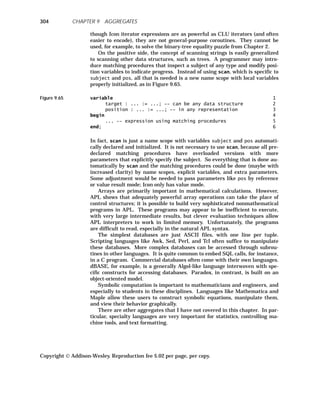
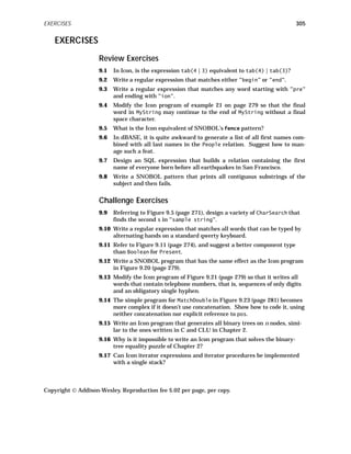
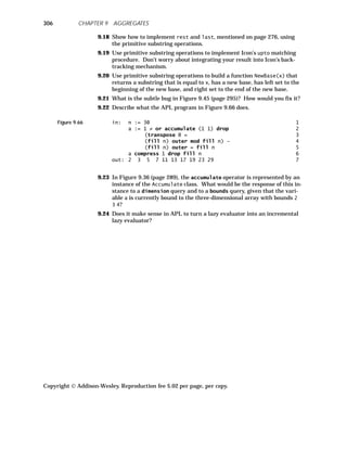
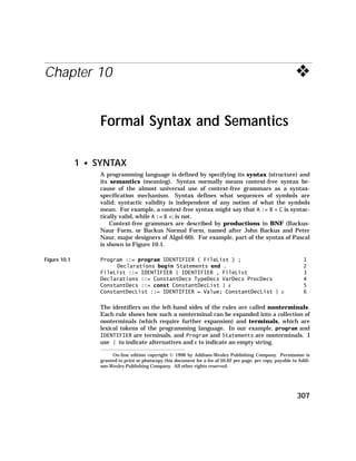
![Sometimes, a clearer notation may be used for BNF; the purpose of nota-
tion, after all, is to specify ideas precisely and clearly. The FileList and Con-
stantDecList productions use recursion to represent arbitrarily long lists. I
can rewrite those productions as shown in Figure 10.2, introducing iteration
for the recursion.
Figure 10.2 FileList ::= [ IDENTIFIER +,] 1
ConstantDecList ::= [ IDENTIFIER = Value ; *] 2
Here I use brackets [ and ] to surround repeated groups. I end the group
either with * , which means 0 or more times (line 2), with + , which means 1
or more times (line 1), or with neither, which means 0 or 1 time. Optionally,
following the * or + is a string that is to be inserted between repetitions. So
line 1 means that there may be one or more identifiers, and if there are more
than one, they are separated by , characters. Line 2 means there may zero
or more constant declarations; each is terminated by the ; character. This
notation obscures whether the repeated items are to be associated to the left
or to the right. If this information is important, it can be specified in some
other way, or the productions can be written in the usual recursive fashion.
The BNF specification is helpful for each of the three software-tool aspects
of a programming language.
1. It helps the programming language designer specify exactly what the
language looks like.
2. It can be used by automatic compiler-generator tools to build the parser
for a compiler.
3. It guides the programmer in building syntactically correct programs.
BNF is inadequate to describe the syntax for some languages. For exam-
ple, Metafont dynamically modifies the meanings of input tokens, so that it is
not so easy to apply standard BNF.
BNF also fails to cover all of program structure. Type compatibility and
scoping rules (for example, that A := B + C is invalid if B or C is Boolean) can-
not be specified by context-free grammars. (Although context-sensitive gram-
mars suffice, they are never used in practice because they are hard to parse.)
Instead of calling this part of program structure static semantics, as has be-
come customary, let me call it advanced syntax. Advanced syntax aug-
ments context-free specifications and completes the definition of what valid
programs look like. Advanced syntax can be specified in two ways:
1. Informally via a programming language report, as is done for most pro-
gramming languages. An informal specification can be compact and
easy to read but is usually imprecise.
2. Formally (for example, via two-level van Wijngaarten grammars or at-
tribute grammars).
Attribute grammars are one popular method of formal specification of ad-
vanced syntax. They formalize the semantic checks often found in compilers.
As an example of attribute grammars, the production E ::= E + T might be
augmented with a type attribute for E and T and a predicate requiring type
compatibility, as shown in Figure 10.3.
Copyright Addison-Wesley. Reproduction fee $.02 per page, per copy.
308 CHAPTER 10 FORMAL SYNTAX AND SEMANTICS](https://image.slidesharecdn.com/advancedprogramminglanguagedesign-230706034617-464d64c2/85/Advanced_programming_language_design-pdf-316-320.jpg)
![309
Figure 10.3 (E2.type = numeric) ∧ (T.type = numeric)
where E2 denotes the second occurrence of E in the production. Attribute
grammars are a reasonable blend of formality and readability, and they are
relatively easy to translate into compilers by standard techniques, but they
can still be rather verbose.
2 ◆ AXIOMATIC SEMANTICS
Semantics are used to specify what a program does (that is, what it com-
putes). These semantics are often specified very informally in a language
manual or report. Alternatively, a more formal operational semantics in-
terpreter model can be used. In such a model, a program state is defined, and
program execution is described in terms of changes to that state. For exam-
ple, the semantics of the statement A := 1 is that the state component corre-
sponding to A is changed to 1. The LISP interpreter presented in Chapter 4 is
operational in form. It defines the execution of a LISP program in terms of
the steps needed to convert it to a final reduced form, which is deemed the re-
sult of the computation. The Vienna Definition Language (VDL) embodies an
operational model in which abstract trees are traversed and decorated to
model program execution [Wegner 72]. VDL has been used to define the se-
mantics of PL/I, although the resulting definition is quite large and verbose.
Axiomatic semantics model execution at a more abstract level than op-
erational models [Gries 81]. The definitions are based on formally specified
predicates that relate program variables. Statements are defined by how
they modify these relations.
As an example of axiomatic definitions, the axiom defining var := exp usu-
ally states that a predicate involving var is true after statement execution if
and only if the predicate obtained by replacing all occurrences of var by exp is
true beforehand. For example, for y > 3 to be true after execution of the state-
ment y := x + 1, the predicate x + 1 > 3 would have to be true before the state-
ment is executed.
Similarly, y = 21 is true after execution of x := 1 if y = 21 is true before its
execution, which is a roundabout way of saying that changing x doesn’t affect
y. However, if x is an alias for y (for example, if x is a formal reference-mode
parameter bound to an actual parameter y), the axiom is invalid. In fact,
aliasing makes axiomatic definitions much more complex. This is one reason
why attempts to limit or ban aliasing are now common in modern language
designs (for example, Euclid and Ada).
The axiomatic approach is good for deriving proofs of program correctness,
because it avoids implementation details and concentrates on how relations
among variables are changed by statement execution. In the assignment ax-
iom, there is no concept of a location in memory being updated; rather, rela-
tions among variables are transformed by the assignment. Although axioms
can formalize important properties of the semantics of a programming lan-
guage, it is difficult to use them to define a language completely. For exam-
ple, they cannot easily model stack overflow or garbage collection.
Denotational semantics is more mathematical in form than operational
semantics, yet it still presents the notions of memory access and update that
are central to von Neumann languages. Because they rely upon notation and
Copyright Addison-Wesley. Reproduction fee $.02 per page, per copy.
2 AXIOMATIC SEMANTICS](https://image.slidesharecdn.com/advancedprogramminglanguagedesign-230706034617-464d64c2/85/Advanced_programming_language_design-pdf-317-320.jpg)
![terminology drawn from mathematics, denotational definitions are often
fairly compact, especially in comparison with operational definitions. Denota-
tional techniques have become quite popular, and a definition for all of Ada
(excluding concurrency) has been written. Indeed, this definition was the ba-
sis for some early Ada compilers, which operated by implementing the deno-
tational representation of a given program.1
A significant amount of effort in
compiler research is directed toward finding automatic ways to convert deno-
tational representations to equivalent representations that map directly to or-
dinary machine code [Wand 82; Appel 85]. If this effort is successful, a
denotational definition (along with lexical and syntactic definitions) may be
sufficient to automatically produce a working compiler.
The field of axiomatic semantics was pioneered by C. A. R. Hoare
[Hoare 69]. The notation
{P} S {R}
is a mathematical proposition about the semantics of a program fragment S.
It means, ‘‘If predicate P is true before program S starts, and program S suc-
cessfully terminates, then predicate R will be true after S terminates.’’
The predicates (P and R) typically involve the values of program variables.
P is called the precondition and R the postcondition of the proposition
above. The precondition indicates the assumptions that the program may
make, and the postcondition represents the result of correct computation. If
P and R are chosen properly, such a proposition can mean that S is a condi-
tionally correct program, which means it is correct if it terminates.
Relatively strong conditions hold for very few program states; relatively
weak conditions hold for very many. The strongest possible condition is false
(it holds for no program state); the weakest possible condition is true (it holds
for every program state). A strong proposition is one with a weak precondi-
tion or a strong postcondition (or both); thus
{true} S {false}
is exceptionally strong. In fact, it is so strong that it is true only of nontermi-
nating programs. It says that no matter what holds before S is executed,
nothing at all holds afterward. Conversely,
{false} S {true}
is an exceptionally weak proposition, true of all programs. It says that given
unbelievable initial conditions, after S finishes, one can say nothing interest-
ing about the state of variables.
hhhhhhhhhhhhhhhhhhhhhhhhhhhhhhhhhhhh
1
The first Ada implementation to take this approach was the NYU Ada/Ed system, infa-
mous for its slowness. Its authors claim this slowness is due primarily to inefficient implemen-
tation of certain denotational functions.
Copyright Addison-Wesley. Reproduction fee $.02 per page, per copy.
310 CHAPTER 10 FORMAL SYNTAX AND SEMANTICS](https://image.slidesharecdn.com/advancedprogramminglanguagedesign-230706034617-464d64c2/85/Advanced_programming_language_design-pdf-318-320.jpg)
![311
2.1 Axioms
The programming language designer can specify the meaning of control
structures by stating axioms, such as the axiom of assignment in Figure 10.4.
Figure 10.4 Axiom of assignment 1
{P[x → y]} x := y {P} 2
where 3
x is an identifier 4
y is an expression without side effects, possibly containing x 5
This notation says that to prove P after the assignment, one must first prove
a related predicate. P[x → y] means the predicate P with all references to x
replaced by references to y. For instance,
{y < 3 ∧ z < y} x := y {x < 3 ∧ z < y}
is a consequence of this axiom.
In addition to axioms, axiomatic semantics contain rules of inference,
which specify how to combine axioms to create provable propositions. They
have the form:
if X and Y then Z
That is, if one already knows X and Y, then proposition Z is proven as well.
Figure 10.5 shows some obvious rules of inference.
Figure 10.5 Rules of consequence 1
if {P} S {R} and R ⇒ Q then {P} S {Q} 2
if {P} S {R} and Q ⇒ P then {Q} S {R} 3
Since R ⇒ S means “R is stronger than S,” the rules of consequence say that
one may always weaken a postcondition or strengthen a precondition. In
other words, one may weaken a proposition that is already proven.
The easiest control structure to say anything about is the composition of
two statements, as in Figure 10.6.
Figure 10.6 Axiom of composition 1
if {P} S1 {Q} and {Q} S2 {R} then {P} S1; S2 {R} 2
Iteration with a while loop is also easy to describe, as shown in Figure
10.7.
Figure 10.7 Axiom of iteration 1
if {P ∧ B} S {P} then 2
{P} while B do S end {¬ B ∧ P} 3
That is, to prove that after the loop B will be false and that P still holds, it suf-
fices to show that each iteration through the loop preserves P, given that B
Copyright Addison-Wesley. Reproduction fee $.02 per page, per copy.
2 AXIOMATIC SEMANTICS](https://image.slidesharecdn.com/advancedprogramminglanguagedesign-230706034617-464d64c2/85/Advanced_programming_language_design-pdf-319-320.jpg)
![holds at the outset of the loop. P is called an invariant of the loop, because
the loop does not cause it to become false.
Figure 10.8 presents an axiom for conditional statements.
Figure 10.8 Axiom of condition 1
if {P ∧ B} S {Q} and {P ∧ ¬B} T {Q} then 2
{P} if B then S else T end {Q} 3
2.2 A Simple Proof
I will now use these axioms to prove a simple program correct. The program
of Figure 10.9 is intended to find the quotient and remainder obtained by di-
viding a dividend by a divisor. It is not very efficient.
Figure 10.9 remainder := dividend; 1
quotient := 0; 2
while divisor ≤ remainder do 3
remainder := remainder - divisor; 4
quotient := quotient + 1 5
end; 6
I would like the predicate shown in Figure 10.10 to be true at the end of this
program.
Figure 10.10 {FINAL: remainder < divisor ∧ 1
dividend = remainder + (divisor * quotient)} 2
The proposition I must prove is {true} Divide {FINAL}. Figure 10.11 pre-
sents a proof.
Figure 10.11 true ⇒ dividend = dividend + divisor * 0 [algebra] 1
{dividend = dividend + divisor*0} remainder := dividend
{dividend = remainder + divisor*0} [assignment] 2
{dividend = remainder + divisor*0} quotient := 0
{dividend = remainder + divisor*quotient} [assignment] 3
{true} remainder := dividend {dividend = remainder+divisor*0}
[consequence, 1, 2] 4
{true} remainder := dividend; quotient := 0
{dividend = remainder+divisor*quotient}
[composition, 3, 4] 5
dividend = remainder+divisor*quotient ∧ divisor ≤ remainder ⇒
dividend=(remainder-divisor)+divisor*(1+quotient)
[algebra] 6
Copyright Addison-Wesley. Reproduction fee $.02 per page, per copy.
312 CHAPTER 10 FORMAL SYNTAX AND SEMANTICS](https://image.slidesharecdn.com/advancedprogramminglanguagedesign-230706034617-464d64c2/85/Advanced_programming_language_design-pdf-320-320.jpg)
![313
{dividend=(remainder-divisor)+divisor*(1+quotient)}
remainder := remainder-divisor
{dividend=remainder+divisor*(1+quotient)} [assignment] 7
{dividend=remainder+divisor*(1+quotient)}
quotient := quotient+1
{dividend=remainder+divisor*quotient} [assignment] 8
{dividend=(remainder-divisor)+divisor*(1+quotient)}
remainder := remainder-divisor; quotient := quotient+1
{dividend=remainder+divisor*quotient}
[composition, 7, 8] 9
{dividend = remainder+divisor*quotient ∧ divisor ≤ remainder}
remainder := remainder-divisor; quotient := quotient+1
{dividend=remainder+divisor*quotient}
[consequence, 6, 9] 10
{dividend = remainder+divisor*quotient}
while divisor≤remainder do
remainder := remainder-divisor;
quotient := quotient+1
end
{remainder < divisor ∧
dividend=remainder+divisor*quotient}
[iteration, 10] 11
{true} Divide {FINAL} [composition, 5, 11] 12
This style of proof is not very enlightening. It is more instructive to deco-
rate the program with predicates in such a way that an interested reader (or
an automated theorem prover) can verify that each statement produces the
stated postcondition given the stated precondition. Each loop needs to be dec-
orated with an invariant. Figure 10.12 shows the same program with decora-
tions.
Figure 10.12 {true} 1
{dividend = dividend + divisor*0} 2
remainder := dividend; 3
{dividend = remainder + divisor*0} 4
quotient := 0; 5
{invariant: dividend = remainder + divisor*quotient} 6
while divisor ≤ remainder do 7
{dividend = (remainder − divisor) + 8
divisor * (quotient+1)} 9
remainder := remainder - divisor; 10
{dividend = remainder + divisor * (quotient + 1)} 11
quotient := quotient + 1 12
{dividend = remainder + divisor * quotient} 13
end; 14
{remainder<divisor ∧ 15
dividend = remainder + (divisor*quotient)} 16
Copyright Addison-Wesley. Reproduction fee $.02 per page, per copy.
2 AXIOMATIC SEMANTICS](https://image.slidesharecdn.com/advancedprogramminglanguagedesign-230706034617-464d64c2/85/Advanced_programming_language_design-pdf-321-320.jpg)
![Unfortunately, the program is erroneous, even though I have managed to
prove it correct! What happens if dividend = 4 and divisor = -2? The while
loop never terminates. The program is only conditionally, not totally, correct.
The idea of axiomatic semantics has proved fruitful. It has been applied
not only to the constructs you have seen, but also to more complex ones such
as procedure and function call, break from a loop, and even goto. Figure
10.13 shows two examples of concurrent programming constructs to which it
has been applied [Owicki 76].
Figure 10.13 Parallel execution axiom 1
if ∀ 0 ≤ i ≤ n, {Pi} Si {Qi}, 2
and no variable free in Pi or Qi is changed in Sj≠i 3
and all variables in I(r) belong to resource r, 4
then 5
{P1 ∧ ... ∧ Pn ∧ I(r)} 6
resource r: cobegin S1 // ... // Sn coend 7
{Q1 ∧... ∧ Qn} 8
Critical section axiom 9
if I(r) is the invariant from the cobegin statement 10
and {I(r) ∧ P ∧ B} S {I(r) ∧ Q) 11
and no variable free in P or Q is changed in 12
another thread 13
then {P} region r await B do S end {Q} 14
The cobegin and region statements are described in Chapter 7. If the formal
axiomatic specification of a construct would suffice to make it intelligible, this
example should require no further clarification. However, it may help to
point out several facts.
• A resource is a set of shared variables.
• The region statement may only appear in a cobegin.
• Region statements for the same resource may not be nested.
The axiomatic method has given rise to an attitude summarized in the fol-
lowing tenets:
1. Programmers should be aware of the propositions that are meant to
hold at different stages of the program.
2. The precondition and the postcondition of each whole program should be
stated explicitly.
3. Students learning to program should write out the loop invariant explic-
itly for each loop.
4. Language constructs that do not have simple axioms (such as goto and
multiple assignment) should not be used.
5. Programmers should prove their programs correct.
6. Proof checkers should be built to assist programmers in proving their
programs correct. Such checkers should understand the axioms and
enough algebra so that only occasional decorations (such as loop invari-
ants) should be needed.
7. Programmers should develop their programs by starting with the post-
condition and working slowly backward, attempting to render it true.
Copyright Addison-Wesley. Reproduction fee $.02 per page, per copy.
314 CHAPTER 10 FORMAL SYNTAX AND SEMANTICS](https://image.slidesharecdn.com/advancedprogramminglanguagedesign-230706034617-464d64c2/85/Advanced_programming_language_design-pdf-322-320.jpg)
![315
8. Programming languages should allow the programmer to explicitly
show loop invariants, preconditions and postconditions to procedure
calls, and other decorations, and the compiler should include a proof
checker.
This attitude has led to extensive research in programming language de-
sign (Alphard and Eiffel were designed with the last point in mind) and auto-
matic theorem provers. However, these tenets are not universally accepted.
The strong argument can be made, for example, that program proofs are only
as good as the precondition/postcondition specification, and that it is just as
easy to introduce a bug in the specifications as it is in the program. For ex-
ample, a sorting routine might have a postcondition that specifies the result
be sorted but might accidentally omit the requirement that the elements be a
permutation of the values in the input. Furthermore, it is hard to put much
faith in an automated proof that is so complex that no human is willing to fol-
low it.
2.3 Weakest Preconditions
The suggestion that a program can itself be developed by attention to the ax-
iomatic meaning of language constructs and that programmers should de-
velop their programs backward was elucidated by Edsger W. Dijkstra
[Dijkstra 75]. Instead of seeing the axioms as static relations between pre-
conditions and postconditions, Dijkstra introduced the concept of weakest
precondition. I will say that P = wp(S, Q) if the following statements hold:
• {P} S {Q}. That is, P is a precondition to S.
• S is guaranteed to terminate, given P. That is, S shows total correct-
ness, not just conditional correctness.
• If {R} S {Q}, then R ⇒ P. That is, P is the weakest precondition, so {P} S
{Q} is the strongest proposition that can be made given S and Q.
Weakest preconditions satisfy several properties:
1. For any statement S, wp(S, false) = false (law of the excluded mira-
cle).
2. If P ⇒ Q, then wp(S, P) ⇒ wp(S, Q) (related to the rules of consequence).
3. wp(S, P) ∧ wp(S, Q) = wp(S, P ∧ Q) (again, related to rules of conse-
quence).
The axioms shown earlier can be restated in terms of wp, as shown in Fig-
ure 10.14.
Figure 10.14 Empty statement 1
wp(skip, R) = R 2
Assignment statement 3
wp(x := y, R) = R[x → y] 4
Composition 5
wp(S1, S2) = wp(S1, wp(S2)) 6
Copyright Addison-Wesley. Reproduction fee $.02 per page, per copy.
2 AXIOMATIC SEMANTICS](https://image.slidesharecdn.com/advancedprogramminglanguagedesign-230706034617-464d64c2/85/Advanced_programming_language_design-pdf-323-320.jpg)
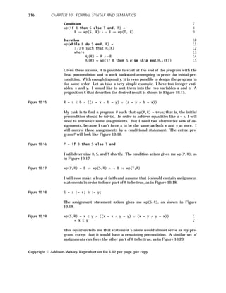
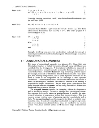
![Stmt → if Expr then Stmt else Stmt
without worrying that not all expressions or statements are valid in an if
statement or that if statements are closed by end to deal with the dangling-
else problem.
Semantic domains define the abstract objects a program manipulates.
These include integers (the mathematical variety, without size limits),
Booleans, and memories (modeled as functions mapping addresses to primi-
tive values). Semantic functions map abstract syntactic structures to corre-
sponding semantic objects. The meaning of a program is the semantic object
produced by the appropriate semantic function. For simple expressions, this
object might be an integer or real; for more complex programs it is a function
mapping input values to output values, or a function mapping memory before
execution to memory after execution.
Concrete examples will make this abstract discussion much clearer. I will
build a denotational description of a programming language by starting with
very simple ideas and enhancing them little by little. As a start, I present in
Figure 10.23 the semantics of binary literals—sequences of 0s and 1s. Be-
cause syntactic and semantic objects often have a similar representation (for
example, 0 can be a binary digit or the integer zero), I will follow the rule that
syntactic objects are always enclosed by [ and ] . The syntactic domain will
be named BinLit and defined by abstract syntax rules. The semantic domain
will be N, the natural numbers. The semantic function will be named E (for
“Expression”) and will map binary literals into natural numbers. The symbol
| separates alternative right-hand sides in productions.
Figure 10.23 Abstract syntax 1
BN ∈ BinLit 2
BN → Seq 3
Seq → 0 | 1 | Seq 0 | Seq 1 4
Semantic domain 5
N = {0,1,2, ...} 6
Semantic function 7
E: BinLit → N 8
E[0] = 0 9
E[1] = 1 10
E[Seq 0] = 2 × E[Seq] 11
E[Seq 1] = 2 × E[Seq] + 1 12
The operators used in the semantic function ( × , + , = ) are standard integer
operators.
I have made a small start at defining the semantics of a programming lan-
guage. At the heart of each denotational-semantics definition is a set of se-
mantic functions. The meaning of a program is, in general, a function
Copyright Addison-Wesley. Reproduction fee $.02 per page, per copy.
318 CHAPTER 10 FORMAL SYNTAX AND SEMANTICS](https://image.slidesharecdn.com/advancedprogramminglanguagedesign-230706034617-464d64c2/85/Advanced_programming_language_design-pdf-326-320.jpg)
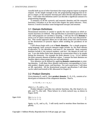
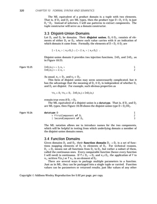
![321
type.
I will need notation for a few simple functions. First, there is the constant
function. For example,
f(x:D) = 17
denotes the function in D → N that always produces the value 17.
Second, I will need a function that differs from an existing function on
only a single parameter value. Suppose f ∈ D1 → D2, x1 ∈ D1, and x2 ∈ D2.
Then
f[x1 ← x2]
denotes the function that differs from f only by producing result x2 on param-
eter x1; that is:
f[x1 ← x2] y = if y = x1 then x2 else f y
This simple device allows me to build up all almost-everywhere-constant
functions—functions that return the same result on all but finitely many dis-
tinct parameter values. This mechanism is particularly useful in modeling
declarations and memory updates.
3.5 Domain Equations
I will define a collection of domains D1, . . . , Dk by a system of formal equa-
tions, as in Figure 10.27.
Figure 10.27 D1 = rhs1 1
... 2
Dk = rhsk 3
Each right-hand side rhsi is a domain expression, built from basic domains
(and possibly from some of the Di themselves) using the domain constructors
given above.
For technical reasons, it is important that I not treat these formal equa-
tions as meaning strict equality. Instead, I use a somewhat more liberal in-
terpretation. I say that domains D1, . . . , Dk comprise a solution to the above
system of domain equations if, for each i, Di is isomorphic to the domain de-
noted by rhsi; that is, there exists a one-to-one, onto function between them.
While I have not shown that this liberal interpretation of domain equa-
tions is technically necessary, you can certainly appreciate its convenience.
Consider the single equation:
D = N ⊕ Bool .
Intuitively, the set N∪Bool has all the properties required of a solution to this
equation. The right-hand side of this equation denotes
Copyright Addison-Wesley. Reproduction fee $.02 per page, per copy.
3 DENOTATIONAL SEMANTICS](https://image.slidesharecdn.com/advancedprogramminglanguagedesign-230706034617-464d64c2/85/Advanced_programming_language_design-pdf-329-320.jpg)
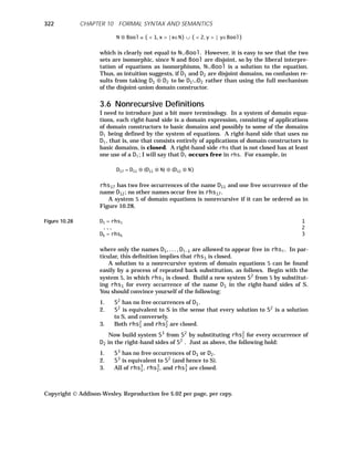
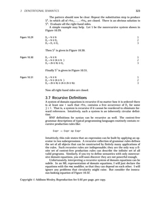
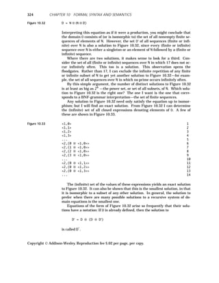
![325
Function domains cause problems in recursive systems of domain equa-
tions. Even a simple recursive equation like
D = . . . ⊕ (D → D) ⊕ . . .
is suspect. Any solution to this equation would have the property that some
subset of itself was isomorphic to its own function space. Unfortunately, if a
set has more than one element, then the cardinality of its function space is
strictly greater than the cardinality of the set itself, so no such isomorphism
is possible!
Am I stuck? Not really. As mentioned above, I interpret D → D to mean
not all functions from D to D, but just a distinguished set of functions called
the continuous ones. There are sufficiently few continuous functions that the
above cardinality argument does not apply, but sufficiently many of them that
all functions computable by programming languages are continuous.
3.8 Expressions
Now that I have discussed domains, I can begin to create richer and more re-
alistic semantic functions. I first extend my definition of binary literals to in-
clude infix operators; see Figure 10.34.
Figure 10.34 Abstract syntax 1
T ∈ Exp 2
T → T + T 3
T → T - T 4
T → T * T 5
T → Seq 6
Seq → 0 | 1 | Seq 0 | Seq 1 7
Semantic domain 8
N = {0,1,2, ..., -1, -2, ...} 9
Semantic function 10
E: Exp → N 11
E[0] = 0 12
E[1] = 1 13
E[Seq 0] = 2 × E[Seq] 14
E[Seq 1] = 2 × E[Seq] + 1 15
E[T1 + T2] = E[T1] + E[T2] 16
E[T1 − T2] = E[T1] − E[T2] 17
E[T1 * T2] = E[T1] × E[T2] 18
This example can be specified in ML as shown in Figure 10.35.
Copyright Addison-Wesley. Reproduction fee $.02 per page, per copy.
3 DENOTATIONAL SEMANTICS](https://image.slidesharecdn.com/advancedprogramminglanguagedesign-230706034617-464d64c2/85/Advanced_programming_language_design-pdf-333-320.jpg)
![Figure 10.35 -- abstract syntax 1
datatype Operator = plus | minus | times; 2
datatype Exp 3
= BinLit of int list -- [0,1] means 10 = 2 4
| Term of Exp*Operator*Exp; 5
-- semantic functions 6
val rec E = 7
fn BinLit([0]) => 0 8
| BinLit([1]) => 1 9
| BinLit(0 :: tail) => 2*E(BinLit(tail)) 10
| BinLit(1 :: tail) => 1+2*E(BinLit(tail)) 11
| Term(x, plus, y) => E(x) + E(y) 12
| Term(x, minus, y) => E(x) - E(y) 13
| Term(x, times, y) => E(x) * E(y); 14
Because it is easier to access the front of a list than the rear, I chose to let
BinLits (line 4) store least-significant bits at the front of the list. A benefit of
the ML description is that it can be given to an ML interpreter to check. For
instance, I have checked the code shown in Figure 10.36.
Figure 10.36 in: E(Term(BinLit([1,1]), plus, 1
BinLit([0,1]))); -- 3 + 2 2
out: 5 : int 3
To include division, I must define what division by zero means. To do so, I
augment the semantic domain with an error element, ⊥. That is, I now have
a domain of R = N ⊕ {⊥}, where R represents “results.” Because this is a dis-
joint-union domain, I can test which subdomain a given semantic element be-
longs to. I use the notation v?D to test if value v is in domain D. I also will
use the following concise conditional-expression notation:
b ⇒ x,y means if b then x else y
Errors must propagate through arithmetic operations, so I need to upgrade
the semantic functions. Figure 10.37 presents the denotation of expressions
with division.
Figure 10.37 Semantic domain 1
R = N ⊕ {⊥} 2
Copyright Addison-Wesley. Reproduction fee $.02 per page, per copy.
326 CHAPTER 10 FORMAL SYNTAX AND SEMANTICS](https://image.slidesharecdn.com/advancedprogramminglanguagedesign-230706034617-464d64c2/85/Advanced_programming_language_design-pdf-334-320.jpg)
![327
Semantic function 3
E: Exp → R 4
E[0] = 0 5
E[1] = 1 6
E[Seq 0] = 2 × E[Seq] 7
E[Seq 1] = 2 × E[Seq] + 1 8
E[T1 + T2] = E[T1]?N ∧ E[T2]?N ⇒ E[T1] + E[T2], ⊥ 9
E[T1 − T2] = E[T1]?N ∧ E[T2]?N ⇒ E[T1] − E[T2], ⊥ 10
E[T1 * T2] = E[T1]?N ∧ E[T2]?N ⇒ E[T1] × E[T2], ⊥ 11
E[T1 / T2] = E[T1]?N ∧ E[T2]?N ⇒ (E[T2] = 0 ⇒ ⊥, E[T1] / E[T2]), ⊥ 12
This definition is unrealistic in that it ignores the finite range of computer
arithmetic. Since I have an error value, I can use it to represent range errors.
I will introduce a function range such that:
range: N → {minInt..maxInt} ⊕ {⊥}. 1
range(n) = minInt ≤ n ≤ maxInt ⇒ n, ⊥ 2
Figure 10.38 shows how to insert Range into the definition of E.
Figure 10.38 Semantic function 1
E: Exp → R 2
E[0] = 0 3
E[1] = 1 4
E[Seq 0] = E[Seq]?N ⇒ range(2 × E[Seq]), ⊥ 5
E[Seq 1] = E[Seq]?N ⇒ range(2 × E[Seq] + 1), ⊥ 6
E[T1 + T2] = E[T1]?N ∧ E[T2]?N ⇒ range(E[T1] + E[T2]), ⊥ 7
E[T1 − T2] = E[T1]?N ∧ E[T2]? ⇒ range(E[T1] − E[T2]), ⊥ 8
E[T1 * T2] = E[T1]?N ∧ E[T2]?N ⇒ range(E[T1] × E[T2]), ⊥ 9
E[T1/T2] = E[T1]?N ∧ E[T2]?N ⇒ 10
(E[T2] = 0 ⇒ ⊥, range(E[T1] / E[T2])), ⊥ 11
It is time to show the ML equivalent, given in Figure 10.39.
Figure 10.39 -- tools 1
val SayError = fn (str, result) => -- report error 2
( output(std_out, str); 3
result -- returned 4
); 5
-- limits 6
val MaxInt = 1000; -- or whatever 7
val MinInt = -1000; -- or whatever 8
Copyright Addison-Wesley. Reproduction fee $.02 per page, per copy.
3 DENOTATIONAL SEMANTICS](https://image.slidesharecdn.com/advancedprogramminglanguagedesign-230706034617-464d64c2/85/Advanced_programming_language_design-pdf-335-320.jpg)
![-- abstract syntax 9
datatype Operator = plus | minus | times | divide; 10
datatype Exp 11
= BinLit of int list -- [0,1] means 10 = 2 12
| Term of Exp*Operator*Exp; 13
-- semantic domains 14
datatype R 15
= NaturalR of int 16
| ErrorR; 17
-- semantic functions 18
val Range = 19
fn NaturalR(a) => 20
if MinInt ≤ a and a ≤ MaxInt then 21
NaturalR(a) 22
else 23
SayError("overflow", ErrorR) 24
| _ => ErrorR; 25
val Add = 26
fn (NaturalR(a),NaturalR(b)) => NaturalR(a+b); 27
val Sub = 28
fn (NaturalR(a),NaturalR(b)) => NaturalR(a-b); 29
val Mul = 30
fn (NaturalR(a),NaturalR(b)) => NaturalR(a*b); 31
val Div = 32
fn (NaturalR(a),NaturalR(0)) => 33
SayError("Divide by zero", ErrorR) 34
| (NaturalR(a),NaturalR(b)) => 35
NaturalR(floor(real(a)/real(b))); 36
val rec E = 37
fn BinLit([0]) => NaturalR(0) 38
| BinLit([1]) => NaturalR(1) 39
| BinLit(0 :: tail) => 40
let val NaturalR(num) = E(BinLit(tail)) 41
in NaturalR(2*num) 42
end 43
| BinLit(1 :: tail) => 44
let val NaturalR(num) = E(BinLit(tail)) 45
in NaturalR(2*num + 1) 46
end 47
| Term(x, plus, y) => Range(Add(E(x), E(y))) 48
| Term(x, minus, y) => Range(Sub(E(x), E(y))) 49
| Term(x, times, y) => Range(Mul(E(x), E(y))) 50
| Term(x, divide, y) => Range(Div(E(x), E(y))); 51
I have introduced an error routine SayError (lines 2–5) so that a user can see
exactly what sort of error has occurred instead of just getting a result of ⊥.
The Range function (lines 19–25) not only checks ranges, but also makes sure
Copyright Addison-Wesley. Reproduction fee $.02 per page, per copy.
328 CHAPTER 10 FORMAL SYNTAX AND SEMANTICS](https://image.slidesharecdn.com/advancedprogramminglanguagedesign-230706034617-464d64c2/85/Advanced_programming_language_design-pdf-336-320.jpg)
![329
that its parameter is a natural number. I have split out Add, Sub, Mul, and
Div (lines 26–36), so that they can check the types of their parameters. I
could have given them alternatives that return ⊥ if the types are not right.
The semantic function E (lines 37–51) needs to convert parameters of type
BinLit to results of type R.
Any realistic programming language will have more than one type, which
I illustrate by adding the semantic domain Bool corresponding to Booleans. I
also add the comparison operator = that can compare two integers or two
Booleans. The additions I need to upgrade Figure 10.38 are given in Figure
10.40.
Figure 10.40 Abstract syntax 1
T → T = T 2
Semantic domain 3
R = N ⊕ Bool ⊕ {⊥} 4
Semantic function 5
E[T1 = T2] = (E[T1]?N ∧ E[T2]?N) ∨ (E[T1]?Bool ∧ E[T2]?Bool) ⇒ 6
(E[T1] = E[T2]), ⊥ 7
3.9 Identifiers
I can now introduce predeclared identifiers, including true and false, max-
int, minint, and so forth. Let Id be the syntactic domain of identifiers, and
let L be a semantic lookup function such that L: Id → V, where
V = N ⊕ Bool ⊕ {udef}. That is, L returns an integer or Boolean value, or
udef if the identifier is undefined. The additions needed for Figure 10.40 are
given in Figure 10.41.
Figure 10.41 Abstract syntax 1
I ∈ Id 2
T → I 3
Semantic domains 4
V = N ⊕ Bool ⊕ {udef} 5
Semantic functions 6
L: Id → V 7
E[I] = L[I]?{udef} ⇒ ⊥, L[I] 8
Copyright Addison-Wesley. Reproduction fee $.02 per page, per copy.
3 DENOTATIONAL SEMANTICS](https://image.slidesharecdn.com/advancedprogramminglanguagedesign-230706034617-464d64c2/85/Advanced_programming_language_design-pdf-337-320.jpg)
![3.10 Environments
The next step is to introduce programmer-defined named constants. This
step requires the concept of an environment that is updated when declara-
tions are made. An environment is a function that maps identifiers (drawn
from the syntactic domain) into results. I will denote the domain of environ-
ments as U, where U = Id → V and V = N ⊕ Bool ⊕ {udef} ⊕ {⊥}, as in Fig-
ure 10.42. If u ∈ U and I ∈ Id, then u[I] is an integer, Boolean, udef, or ⊥,
depending on how and whether I has been declared. I can incorporate the
definition of predeclared named constants by including them in u0, a prede-
fined environment. I no longer need the lookup function L.
Figure 10.42 Semantic domain 1
V = N ⊕ Bool ⊕ {udef} ⊕ {⊥} 2
U = Id → V 3
Semantic functions 4
E[I] = u0[I]?{udef} ⇒ ⊥, u0[I] 5
The environment approach is useful because environments can be computed
as the results of semantic functions (those that define the meaning of a local
constant declaration).
It is time to expand my abstract syntax for a program into a sequence of
declarations followed by an expression that yields the result of a program. I
can specify whatever I like for the meaning of a redefinition of an identifier.
In Figure 10.43, redefinitions will have no effect.
I will introduce two new semantic functions: D, which defines the semantic
effect of declarations, and M, which defines the meaning of a program. D is
curried; it maps a declaration and an old environment into a new environ-
ment in two steps. There is a major change to E; it now maps an expression
and an environment into a result. Pr is the syntactic domain of all programs;
Decls is the syntactic domain of declarations.
Figure 10.43 Abstract syntax 1
P ∈ Pr -- a program 2
T ∈ Exp -- an expression 3
I ∈ Id -- an identifier 4
Def ∈ Decls -- a declaration 5
P → Def T 6
Def → ε -- empty declaration 7
Def → I = T ; -- constant declaration 8
Def → Def Def -- declaration list 9
T → I -- identifier expression 10
Copyright Addison-Wesley. Reproduction fee $.02 per page, per copy.
330 CHAPTER 10 FORMAL SYNTAX AND SEMANTICS](https://image.slidesharecdn.com/advancedprogramminglanguagedesign-230706034617-464d64c2/85/Advanced_programming_language_design-pdf-338-320.jpg)
![331
Semantic domains 11
R = N ⊕ Bool ⊕ {⊥} -- program results 12
V = N ⊕ Bool ⊕ {udef} ⊕ {⊥} -- lookup values 13
U = Id → V -- environments 14
Semantic functions 15
E: Exp → U → R 16
D: Decls → U → U 17
M: Pr → R 18
M[Def T] = E[T]u 19
where u = D[Def]u0. 20
D[ε]u = u 21
D[I = T]u = u[I]?{udef} ⇒ u[I ← e], u 22
where e = E[T]u. 23
D[Def1 Def2] u = D[Def2]v 24
where v = D[Def1]u. 25
E[I] = u[I] ?{udef} ⇒ ⊥, u[I] 26
E[0]u = 0 27
E[1]u = 1 28
E[Seq 0] u = E[Seq]u?N ⇒ range(2 × E[Seq]u), ⊥ 29
E[Seq 1] u = E[Seq]u?N ⇒ range(2 × E[Seq]u + 1), ⊥ 30
E[T1 + T2] u = E[T1]u?N ∧ E[T2]u?N ⇒ 31
range(E[T1] u + E[T2]u), ⊥ 32
E[T1 − T2] u = E[T1]u?N ∧ E[T2]u?N ⇒ 33
range(E[T1] u − E[T2]u), ⊥ 34
E[T1 * T2] u = E[T1]u?N ∧ E[T2]u?N ⇒ 35
range(E[T1] u × E[T2]u), ⊥ 36
E[T1 / T2] u = E[T1]u?N ∧ E[T2]u?N ⇒ 37
(E[T2] u = 0 ⇒ ⊥, range(E[T1] u / E[T2]u)), ⊥ 38
E[T1 = T2]u = (E[T1]u?N ∧ E[T2]u?N) ∨ (E[T1]u?Bool ∧ E[T2]u?Bool) ⇒ 39
(E[T1]u = E[T2]u), ⊥ 40
Lines 19–20 define the meaning of a program to be the value of the expres-
sion T in the environment u formed by modifying the initial environment u0
by the declarations. Lines 22–23 show how declarations modify a given envi-
ronment u by substituting the meaning of T for the identifier I in u. Multiple
declarations build the final environment in stages (lines 24–25).
Line 22 explicitly ignores attempts to redefine an identifier, but I can
make the language a bit more realistic. I will let a redefinition of an identi-
fier return an environment in which the identifier is bound to a new kind of
error value named redef. E of a redefined identifier will yield ⊥. I extend the
domain V of possible environment values to include redef. Figure 10.44
shows the differences.
Copyright Addison-Wesley. Reproduction fee $.02 per page, per copy.
3 DENOTATIONAL SEMANTICS](https://image.slidesharecdn.com/advancedprogramminglanguagedesign-230706034617-464d64c2/85/Advanced_programming_language_design-pdf-339-320.jpg)
![Figure 10.44 Semantic domains 1
V = N ⊕ Bool ⊕ {⊥} ⊕ {udef} ⊕{redef} 2
Semantic functions 3
D[I = T]u = u[I]?{udef} ⇒ u[I ← e], u[I ← redef] 4
where e = E[T]u. 5
E[I]u = u[I]?({udef} ⊕ {redef}) ⇒ ⊥, u[I] 6
At this point I could add block structure, but since programs only compute
a single expression, scoping isn’t needed yet. Instead, I will put in variables.
3.11 Variables
I can model variables in several ways. The most general model employs an
environment that maps identifiers to locations and a store that maps loca-
tions to values. This is how most languages are implemented, and it would
allow me to model aliasing, reuse of storage, and so forth.
For the present, I’ll use a simpler interpreter model and continue to use
the environment function to map identifiers directly to values. I will also
store a flag that indicates if a value can be changed (that is, if it’s an L-value,
not an R-value). An interpreter does roughly the same thing, maintaining a
runtime symbol table for all program variables. From the semantic point of
view, the distinction between interpreters and compilers is irrelevant—what
is important is what the answer is, not how it’s produced. The interpreter ap-
proach will allow interesting variations. For example, an untyped language
(like Smalltalk) is just as easy to model as a strongly typed language.
I begin by extending the environment domain U as in Figure 10.45 to in-
clude an indication of how an identifier can be used:
U = Id → {var, const, uninit} ⊗ V
Uninit models the fact that after a variable is declared, it may be assigned to,
but not yet used. After a variable is assigned a value, its flag changes from
uninit to var. It is time to introduce statements. (In denotational for-
malisms, statements are usually called commands.) A statement maps an en-
vironment into a new environment (or ⊥). That is,
S: Stm → U → (U ⊕ {⊥})
where S is the semantic function for statements, and Stm is the syntactic do-
main of statements.
I will first add only variable declarations and assignment statements to
the programming language. Since there is no I/O, I will define the result of
the program to be the final value of an identifier that is mentioned in the pro-
gram header, as in Figure 10.45, which produces 1 as its result.
Copyright Addison-Wesley. Reproduction fee $.02 per page, per copy.
332 CHAPTER 10 FORMAL SYNTAX AND SEMANTICS](https://image.slidesharecdn.com/advancedprogramminglanguagedesign-230706034617-464d64c2/85/Advanced_programming_language_design-pdf-340-320.jpg)
![Semantic functions 20
E: Exp → U → R 21
D: Decls → U → U 22
M: Pr → R 23
S: Stm → U → (U ⊕ {⊥}) 24
M[program (I) Def St end] = c?U ⇒ E[I]c, ⊥ 25
where u = D[Def]u0; c = S[St]u. 26
D[ε]u = u 27
D[I = T]u = u[I]?{udef} ⇒ u[I ← f], u[I ← redef] 28
where e = E[T]u; f = e?⊥ ⇒ ⊥, < const, e > . 29
D[I: integer]u = u[I]?{udef} ⇒ u[I ← e], u[I ← redef] 30
where e = <uninit, InN(0)> 31
D[I: Boolean]u = u[I]?{udef} ⇒ u[I ← e], u[I ← redef] 32
where e = <uninit, InBool(true)>. 33
D[Def1 Def2]u = D[Def2]v 34
where v = D[Def1]u. 35
E[I]u = v?({redef} ⊕ {udef} ⊕ {⊥}) ⇒ ⊥, 36
(Hd(v) = uninit ⇒ ⊥, Tl(v)) 37
where v = u[I]. 38
S[ε]u = u 39
S[I: = T]u = v?({redef}⊕{udef}⊕{⊥}) ∨ (Hd(v) = const) ∨ e?{⊥} ⇒ 40
⊥, (e?N ∧ Tl(v)?N) ∨ (e?Bool ∧ Tl(v)?Bool) ⇒ 41
u[I ← < var, e >], ⊥ 42
where e = E[T]u; v = u[I]. 43
S[St1 St2] u = g?U ⇒ S[St2]g, ⊥ 44
where g = S[St1]u. 45
The easiest way to read the semantic functions is to first look at the where
clauses to see the local shorthands. (These are like ML let blocks.) Then
look at the definition itself, following the case where no errors are encoun-
tered. Much of each definition necessarily deals with checking for error situ-
ations, which tend to confuse the central issue. When I describe definitions, I
will generally ignore all the error cases and concentrate on the usual case.
Lastly, assure yourself that the functions are given parameters of the correct
domains and produce results in the correct domains.
For example, lines 40–43 describe what an assignment does to the envi-
ronment u. Start with line 43. The local variable e stands for the value of
the right-hand side of the assignment in environment u, and v stands for the
meaning of the identifier on the left-hand side. This meaning is evaluated in
the same environment u, so if evaluating the right-hand side had a side effect
(it can’t yet, but it might later), that effect is ignored in determining the iden-
tifier’s meaning. Then (line 40) given that v is properly declared and not a
constant, given that e evaluates successfully, and given (line 41) that the ex-
pression and identifier are the same type, the statement creates a new envi-
ronment (line 42) that is just like the old one with the identifier reassigned.
To check domain consistency, I will ignore all error cases and write out
these few lines again in Figure 10.47.
Copyright Addison-Wesley. Reproduction fee $.02 per page, per copy.
334 CHAPTER 10 FORMAL SYNTAX AND SEMANTICS](https://image.slidesharecdn.com/advancedprogramminglanguagedesign-230706034617-464d64c2/85/Advanced_programming_language_design-pdf-342-320.jpg)
![335
Figure 10.47 S[I: = T]u = u[I ← < var, e >] 1
where e = E[T]u. 2
Now I can painstakingly infer the type of S, as shown in Figure 10.48.
Figure 10.48 E: Exp → U → R 1
E[T]: U → R 2
e = E[T]u: R 3
e: V, since V is a superset of R 4
u: U 5
u: Id → {var, const, uninit} ⊗ V 6
u[I]: {var, const, uninit} ⊗ V 7
< var, e > : {var, const, uninit} ⊗ V 8
u[I ← < var, e >]: U 9
u[I ← < var, e >]: U ⊕ {⊥}, which is a superset of U 10
S: Stm → U → (U ⊕ {⊥}) 11
S[I: = T]: U → (U ⊕ {⊥}) 12
S[I: = T]u: U ⊕ {⊥} 13
Line 10 shows the type of the right-hand side of the equation in line 1, and
line 13 shows the type of the left-hand side. They match. It was necessary to
raise several types; see lines 4 and 10. If this example were coded in ML, I
would need to use explicit type converters.
Other notes on Figure 10.46: The value of 0 in line 31 is arbitrary since I
don’t allow access to variables with an uninit flag. In the definition of state-
ment execution (lines 43–44), as soon as a statement yields ⊥, all further
statement execution is abandoned.
As I suggested earlier, my definitions can easily be modified to handle un-
typed languages like Smalltalk. I would of course modify the variable-
declaration syntax to omit the type specification. A variable would assume
the type of the object assigned to it. The definitions of E and S would be writ-
ten as in Figure 10.49.
Figure 10.49 E[I]u = v?({redef} ⊕ {udef} ⊕ {⊥}) ⇒ ⊥, Tl(v) 1
where v = u[I]. 2
S[I: = T]u = v?({redef}⊕{⊥}) ∨ (Hd(v) = const) ∨ e?{⊥} ⇒ 3
⊥, u[I ← < var, e >] 4
where e = E[T]u; v = u[I]. 5
3.12 Conditional and Iterative Statements
Conditional execution and iterative execution for a fixed number of iterations
are readily modeled with the additions to the previous definition shown in
Figure 10.50.
Copyright Addison-Wesley. Reproduction fee $.02 per page, per copy.
3 DENOTATIONAL SEMANTICS](https://image.slidesharecdn.com/advancedprogramminglanguagedesign-230706034617-464d64c2/85/Advanced_programming_language_design-pdf-343-320.jpg)
![Figure 10.50 Abstract syntax 1
St → if T then St else St 2
St → do T times St 3
Semantic functions 4
S[if T then St1 else St2]u = e?Bool ⇒ 5
(e ⇒ S[St1]u, S[St2]u), ⊥ 6
where e = E[T]u. 7
S[do T times St]u = e?N ⇒ vm , ⊥ 8
where e = E[T]u; m = max(0, e); v0 = u; 9
vi+1 = vi?U ⇒ S[St]vi, ⊥. 10
In lines 8–10, vi is the environment after i iterations of the loop.
The semantic definition of a while loop requires special care. The problem
is that some while loops will never terminate, and I would like a mathemati-
cally sound definition of all loops. I might try to build on the definition for
the do loop, but for nonterminating loops that would create an infinite se-
quence of intermediate environments (vi’s).
I will follow standard mathematical practice for dealing with infinite se-
quences and try to determine if a limit exists. I will then be able to conclude
that infinite loops have a value of ⊥, though the semantic function for while
loops will not always be computable (because of decidability issues). Follow-
ing Tennent, I will define a sequence of approximations to the meaning of a
while loop [Tennent 81].
Let p0 ≡ ⊥. This formula represents a while loop whose Boolean expres-
sion has been tested zero times. Since a loop can’t terminate until its Boolean
expression has evaluated to false, p0 represents the base state in which the
definition hasn’t yet established termination. Now I define pi+1 recursively,
as in Figure 10.51.
Figure 10.51 pi+1(u) = e?Bool ⇒ (e ⇒ (v?{⊥}⇒⊥, pi(v)), u), ⊥ 1
where e = E[T]u; v = S[St]u. 2
If a while loop terminates without error after exactly one evaluation of the
control expression (because the expression is initially false), p1(u) returns u
(the environment after zero iterations through the loop). In all other cases,
p1(u) returns ⊥.
If a while loop terminates without error after at most two evaluations of
the control expression, p2(u) returns v, the environment after loop termina-
tion. In all other cases, p2(u) returns ⊥. In general, if a loop terminates after
n iterations, pm(u) for m ≥ n will yield the environment after termination,
given an initial environment u. For all terminating loops, the limit of pi(u) as
i → ∞ is the environment after loop termination. If the loop doesn’t termi-
nate or encounters a runtime error, then all pi’s return ⊥, which is then triv-
ially the limit as i → ∞. The sequence of pi’s always converges, so the limit is
always defined. This leads to the definition of a while loop given in Figure
10.52.
Copyright Addison-Wesley. Reproduction fee $.02 per page, per copy.
336 CHAPTER 10 FORMAL SYNTAX AND SEMANTICS](https://image.slidesharecdn.com/advancedprogramminglanguagedesign-230706034617-464d64c2/85/Advanced_programming_language_design-pdf-344-320.jpg)
![337
Figure 10.52 S[while T do St]u =
i→∞
lim pi(u) 1
where pi+1(w) = e?Bool ⇒ (e ⇒ (v?{⊥} ⇒ ⊥, pi(v)), w), ⊥; 2
e = E[T]w; v = S[St]w. 3
In general, the above limit is not computable (because the halting problem is
undecidable), but the limit can be computed for some infinite loops (and all fi-
nite loops). For example, it doesn’t take an oracle to decide that the loop in
Figure 10.53 has some problems.
Figure 10.53 while true do 1
x := x + 1 2
What does the denotational definition say about this loop? Assuming true
hasn’t been redefined, the semantic function is shown in Figure 10.54.
Figure 10.54 pi+1(u) = (true ⇒ (v?{⊥} ⇒ ⊥, pi(v)), u) = v?{⊥} ⇒ ⊥, pi(v) 1
where v = S[St]u. 2
Now, pi+1(u) is either equal to ⊥ or pi(v). Similarly, pi(v) is either equal to ⊥
or pi−1(v′). But p0(s) ≡ ⊥ for all s, so each pi must reduce to ⊥, so ⊥ is the
limit of the sequence. The loop fails either because x overflows or because the
loop doesn’t terminate. Since both failings are represented by ⊥, the denota-
tional definition has correctly handled this example.
3.13 Procedures
I now consider simple procedures of the abstract form shown in Figure 10.55.
Figure 10.55 procedure I; 1
St 2
Procedures are invoked by a call statement (for example, call I). Since
there are no scope rules yet, a procedure invocation is equivalent to macro
substitution and immediate execution of the procedure’s body. A procedure
can call another procedure, but I will forbid recursion for now. Since a proce-
dure name is a synonym for a list of statements, it represents a mapping from
an environment to an updated environment or to ⊥. The semantic domain for
procedure declarations is given in Figure 10.56.
Figure 10.56 Proc = U → (U ⊕ {⊥})
I need to upgrade the environment domain to include procedures, as well as
introduce a new flag opencall. I will set opencall when a procedure call is
in progress, but not yet completed. To prevent recursion, I will disallow in-
voking a procedure that has opencall set. The environment domain U is now
as shown in Figure 10.57.
Copyright Addison-Wesley. Reproduction fee $.02 per page, per copy.
3 DENOTATIONAL SEMANTICS](https://image.slidesharecdn.com/advancedprogramminglanguagedesign-230706034617-464d64c2/85/Advanced_programming_language_design-pdf-345-320.jpg)
![Figure 10.57 V = N ⊕ Bool ⊕ Proc ⊕ {⊥} ⊕ {udef} ⊕{redef} -- id value 1
U = Id → {var, const, uninit, opencall} ⊗ V -- environments 2
These domain equations are recursive: U references Proc, and Proc refer-
ences U. Before, I used f[x ← y] to denote the function equal to f for all pa-
rameters except x, where y is to be returned. In the case that y is a member
of a product domain, I will extend the notation;
f[Hd[x ← y]]
will denote the function equal to f for all parameters except x, where
Hd(f(x)) = y, but Tl(f(x)) is unchanged; f[Tl[x ← y]] will have an analo-
gous definition. Figure 10.58 gives the new part of the definition, building on
Figure 10.46 (page 333).
Figure 10.58 Abstract syntax 1
Def → procedure I; St 2
St → call I 3
Semantic domains 4
Proc = U → (U ⊕ {⊥}) -- procedure declaration 5
V = N ⊕ Bool ⊕ Proc ⊕ {⊥} ⊕ {udef} ⊕{redef} -- id value 6
U = Id → {var, const, uninit, opencall} ⊗ V -- environments 7
Semantic functions 8
D[procedure I; St]u = u[I]?{udef} ⇒ u[I ← c], u[I ← redef] 9
where c = < const, InProc(S[St]) > . 10
S[call I]u = Tl(v)?Proc ∧ Hd(v) = const ∧ w?U ⇒ 11
w[Hd[I ← const]], ⊥ 12
where v = u[I]; w = Tl(v)(u[Hd[I ← opencall]]); 13
A procedure declaration (lines 9–10) updates the current environment u by
calculating the meaning of the body St and converting the result to domain
Proc (line 10). This result is used to build a meaning for I in the environ-
ment (line 9). The definition of procedure invocation in lines 11–13 first mod-
ifies I in the environment u to indicate the call is open, then applies the body
of procedure I (Tl(v) in line 13), storing the resulting environment in w. It
then returns w, but first restores the definition of I (line 12).
3.14 Functions
Functions, like procedures, execute a list of statements. They also return a
value by evaluating an expression immediately prior to return. For the pre-
sent, I will constrain functions to be nonrecursive. The abstract syntax of in-
teger functions will be as shown in Figure 10.59.
Copyright Addison-Wesley. Reproduction fee $.02 per page, per copy.
338 CHAPTER 10 FORMAL SYNTAX AND SEMANTICS](https://image.slidesharecdn.com/advancedprogramminglanguagedesign-230706034617-464d64c2/85/Advanced_programming_language_design-pdf-346-320.jpg)
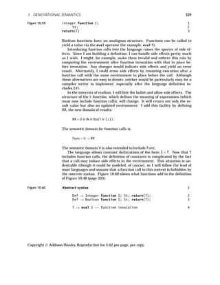
![Semantic domains 5
RR = U ⊗ (N ⊕ Bool ⊕ {⊥}) -- expression result 6
Func = U → RR 7
V = N ⊕ Bool ⊕ Proc ⊕ Func {⊥} ⊕ {udef} ⊕{redef} -- id value 8
U = Id → {var, const, uninit, opencall} ⊗ V -- environments 9
Semantic functions 10
E: Exp → U → RR 11
M[program (I) Def St end] = c?U ⇒ Tl(E[I]c), ⊥ 12
where u = D[Def]u0; c = S[St]u. 13
D[I = T]u = u[I]?{udef} ⇒ u[I ← f], u[I ← redef] 14
where e = E[T]u; f = e?{⊥} ⇒ ⊥, < const, Tl(e) > . 15
D[Integer function I; St; return(T)]u = 16
u[I]?{udef} ⇒ u[I ← f], u[I ← redef] 17
where f = < const, InFunc(v) > ; c = S[St]; e(w) = E[T](c(w)); 18
v(w) = c(w)?{⊥} ∨ e(w)?{⊥} ⇒ ⊥, (Tl(e(w))?N ⇒ e(w), ⊥). 19
D[Boolean function I; St; return(T)]u = 20
u[I]?{udef} ⇒ u[I ← f], u[I ← redef] 21
where f = < const, InFunc(v) > ; c = S[St]; e(w) = E[T](c(w)); 22
v(w) = c(w)?{⊥} ∨ e(w)?{⊥} ⇒ ⊥, (Tl(e(w))?Bool ⇒ e(w), ⊥). 23
E[0]u = < u, 0 > 24
E[1]u = < u, 1 > 25
E[Seq 0] u = e?N ∧ range(2 × e)?N ⇒ < u, 2 × e > , ⊥ 26
where e = Tl(E[Seq]u). 27
E[Seq 1] u = e?N ∧ range(2 × e + 1)?N ⇒ < u, 2 × e + 1 > , ⊥ 28
where e = Tl(E[Seq]u). 29
E[T1 + T2] u = Tl(e)?N ∧ Tl(f)?N ∧ 30
range(Tl(e) + Tl(f))?N ⇒ < Hd(f), Tl(e) + Tl(f) > , ⊥ 31
where e = E[T1]u; f = E[T2]Hd(e). 32
E[T1 − T2] u = Tl(e)?N ∧ Tl(f)?N ∧ 33
range(Tl(e) − Tl(f))?N ⇒ < Hd(f), Tl(e) − Tl(f) > , ⊥ 34
where e = E[T1]u; f = E[T2]Hd(e). 35
E[T1 * T2] u = Tl(e)?N ∧ Tl(f)?N ∧ 36
range(Tl(e) × Tl(f))?N ⇒ < Hd(f), Tl(e) × Tl(f) > , ⊥ 37
where e = E[T1]u; f = E[T2]Hd(e). 38
E[T1 / T2] u = Tl(e)?N ∧ Tl(f)?N ∧ Tl(f)≠0 ∧ 39
range(Tl(e) / Tl(f))?N ⇒ < Hd(f), Tl(e)/Tl(f) > , ⊥ 40
where e = E[T1]u; f = E[T2]Hd(e). 41
E[T1 = T2] u = (Tl(e)?N ∧ Tl(f)?N) ∨ (Tl(e)?Bool ∧ Tl(f)?Bool) ⇒ 42
< Hd(f), (Tl(e) = Tl(f)) > , ⊥ 43
where e = E[T1]u; f = E[T2]Hd(e). 44
E[eval I]u = Tl(v)?Func ∧ Hd(v) = const ∧ w≠⊥ ⇒ 45
w[Hd[I ← const]], ⊥ 46
where v = u[I]; w = Tl(v)(u[Hd[I ← opencall]]). 47
E[I]u = v?({redef} ⊕ {⊥} ⊕{udef}) ⇒ ⊥, 48
(Hd(v) = uninit ⇒ ⊥, < u, Tl(v) >) 49
where v = u[I]. 50
Copyright Addison-Wesley. Reproduction fee $.02 per page, per copy.
340 CHAPTER 10 FORMAL SYNTAX AND SEMANTICS](https://image.slidesharecdn.com/advancedprogramminglanguagedesign-230706034617-464d64c2/85/Advanced_programming_language_design-pdf-348-320.jpg)
![341
S[I: = T]u = v?({redef} ⊕ {⊥} ⊕{udef}) ∨ 51
(Hd(v) = const) ∨ e?{⊥} ⇒ ⊥, 52
(Tl(e)?N ∧ Tl(v)?N) ∨ (Tl(e)?Bool ∧ Tl(v)?Bool) ⇒ 53
Hd(e)[I ←< var, Tl(e) >], ⊥ 54
where e = E[T]u; v = u[I]. 55
S[if T then St1 else St2]u = 56
Tl(e)?Bool ⇒ (Tl(e) ⇒ S[St1]Hd(e), S[St2]Hd(e)), ⊥ 57
where e = E[T]u. 58
S[do T times St]u = Tl(e)?N ⇒ vm(Hd(e)), ⊥ 59
where e = E[T]u; m = max(0, Tl(e)); 60
v0(w) = w; vi+1(w) = vi(w)?U ⇒ S[St]vi(w), ⊥. 61
S[while T do St]u =
i → ∞
lim pi(u) 62
where p0(w) = ⊥; 63
pi+1(w) = Tl(e)?Bool ⇒ 64
(Tl(e) ⇒ (v?{⊥} ⇒ ⊥, pi(v)), Hd(e)), ⊥; 65
e = E[T]w; v = S[St]Hd(e). 66
In line 14, I assume that the concrete syntax forbids function calls in the defi-
nition of a constant.
3.15 Recursive Routines
The danger in allowing recursive routines is that the definitions may become
circular. As it stands, I define the meaning of a call in terms of the meaning
of its body. If recursion is allowed, the meaning of a routine’s body may itself
be defined in terms of any calls it contains. My current definition breaks this
potential circularity by forbidding calls of a routine (directly or indirectly)
from its own body.
I will generalize the definition of a subroutine call to allow calls of
bounded depth. The meaning of a routine with a maximum call depth of n
will be defined in terms of the meaning of the subroutine’s body with subse-
quent calls limited to a depth of n−1. The meaning of a call with a maximum
depth of zero is ⊥.
If a call to a routine will ever return, then it can be modeled by a call lim-
ited to depth n as long as n is sufficiently large. As n approaches ∞, the
bounded-call-depth model converges to the unbounded-call model if the latter
ever returns. But if a routine call doesn’t ever return, then the bounded-call-
depth model will always produce an error result ⊥, which is a correct defini-
tion of an infinite recursion. Thus the limit as n approaches ∞ of the
bounded-call-depth model is ⊥, which I will take as the definition of the
meaning of a call of unbounded depth that never returns. This approach par-
allels how I handled unbounded iteration, which isn’t surprising, given the
similarity of looping and subroutine call.
I will redefine U to replace the opencall flag with an integer representing
the maximum depth to which a given procedure or function can be called. If
this value is zero, the call is invalid. What used to be opencall is now repre-
sented by 0; the previous model always had a maximum call depth of 1. Fig-
ure 10.61 shows the necessary additions.
Copyright Addison-Wesley. Reproduction fee $.02 per page, per copy.
3 DENOTATIONAL SEMANTICS](https://image.slidesharecdn.com/advancedprogramminglanguagedesign-230706034617-464d64c2/85/Advanced_programming_language_design-pdf-349-320.jpg)
![Figure 10.61 U = Id → ({var, const, uninit} ⊕ N) ⊗ V 1
S[call I]u = Tl(v)?Proc ⇒
i → ∞
lim pi(u, v), ⊥ 2
where v = u[I]; 3
p0(u′, v′) = ⊥; 4
pi+1(u′, v′) = Hd(v′) = const ⇒ (w?U ⇒ w[Hd[I ← const]], ⊥), 5
Hd(v′) > 0 ∧ y?U ⇒ y[Hd[I ← Hd(v′)]], ⊥; 6
w = Tl(v′)(u′[Hd[I ← i]]); 7
y = Tl(v′)(u′[Hd[I ← Hd(v′) − 1]]). 8
E[eval I]u = Tl(v)?Func ⇒
i → ∞
lim pi(u, v), ⊥ 9
where v = u[I]; 10
p0(u′, v′) = ⊥; 11
pi+1(u′, v′) = Hd(v′) = const ⇒ (w≠⊥{⊥}⇒{⊥} 12
w[Hd[I ← const]], ⊥), 13
Hd(v′) > 0 ∧ y≠⊥ ⇒ y[Hd[I ← Hd(v′)]], ⊥; 14
w = Tl(v′)(u′[Hd[I ← i]]); 15
y = Tl(v′)(u′[Hd[I ← Hd(v′) − 1]]). 16
3.16 Modeling Memory and Files
I am now ready to model variables more accurately. I will use a finite seman-
tic domain Loc to name addressable memory locations. A semantic domain
Mem will model memories as a mapping from Loc to an integer or Boolean
value or to error values uninitInt, uninitBool, unalloc:
Mem = Loc → N ⊕ Bool ⊕ uninitInt ⊕ uninitBool ⊕ unalloc
The uninitialized flag will now be in the memory mapping, not the environ-
ment mapping. Two different uninit flags are used to remember the type an
uninitialized location is expected to hold. If a memory location is marked as
unalloc, then it can be allocated for use (and possibly deallocated later). If
m ∈ Mem, then I define alloc as follows:
alloc(m) = any l ∈ Loc such that m(l) = unalloc
= ⊥ if no such l exists
Alloc specifies no particular memory allocation pattern; this definition allows
implementations the widest latitude in memory management.
I will model files as finite sequences over integers, Booleans, and eof, the
end-of-file flag. I define the semantic domain File as:
File = (N ⊕ Bool ⊕ eof) *
That is, a file is a potentially infinite string of typed values. My definitions
will never consider values in files following the first eof. Programs will now
take an input file and produce an output file (or ⊥). To model this semantics,
I will have a semantic domain State that consists of a memory and a pair of
files:
Copyright Addison-Wesley. Reproduction fee $.02 per page, per copy.
342 CHAPTER 10 FORMAL SYNTAX AND SEMANTICS](https://image.slidesharecdn.com/advancedprogramminglanguagedesign-230706034617-464d64c2/85/Advanced_programming_language_design-pdf-350-320.jpg)
![343
State = Mem ⊗ File ⊗ File
At any point during execution, the current state is a combination of the cur-
rent memory contents, what is left of the input file, and what has been writ-
ten to the output file.
My definition of environments will now more nearly match the symbol ta-
bles found in conventional compilers. I will map identifiers to constant val-
ues, locations or routines:
V = N ⊕ Bool ⊕ Loc ⊕ Proc ⊕ Func ⊕ {⊥} ⊕ {udef} ⊕ {redef}
U = Id → V
Statements will take an environment and a state and will produce an up-
dated state or an error value. Declarations will take an environment and
state and will produce an updated environment and state (since memory allo-
cation, performed by declarations, will update the original state). Figure
10.62 shows the additions and changes to the formal definition.
Figure 10.62 Abstract syntax 1
P → program Def St end -- program 2
St → read I -- read statement 3
St → write T -- write statement 4
Semantic domains 5
State = Mem ⊗ File ⊗ File 6
RR = State ⊗ (N ⊕ Bool ⊕ {⊥}) 7
Proc = (U → State → (State ⊕ {⊥})) ⊗ Loc 8
Func = (U → State → RR) ⊗ Loc 9
Mem = Loc → N ⊕ Bool ⊕ {uninitInt} ⊕ {uninitBool} ⊕ 10
{unalloc} 11
File = (N ⊕ Bool ⊕ {eof}) * 12
V = N ⊕ Bool ⊕ Loc ⊕ Proc ⊕ Func ⊕ {⊥}⊕{udef}⊕{redef} 13
U = Id → V 14
Semantic functions 15
E: Exp → U → State → RR 16
D: Decls → (U ⊗ State) → (U ⊗ State) 17
M: Pr → File → File ⊕ {⊥} 18
S: Stm → U → State → (State ⊕ {⊥}) 19
E[0] u s = < s, 0 > 20
E[1] u s = < s, 1 > 21
E[Seq0] u s = e?N ∧ range(2 × e)?N ⇒ < s, 2 × e > , ⊥ 22
where e = Tl(E[Seq] u s). 23
E[Seq1] u s = e?N ∧ range(2 × e + 1)?N ⇒ < s, 2 × e + 1 > , ⊥ 24
where e = Tl(E[Seq] u s). 25
Copyright Addison-Wesley. Reproduction fee $.02 per page, per copy.
3 DENOTATIONAL SEMANTICS](https://image.slidesharecdn.com/advancedprogramminglanguagedesign-230706034617-464d64c2/85/Advanced_programming_language_design-pdf-351-320.jpg)
![E[I] u s = v?({⊥} ⊕ {redef} ⊕ {udef}) ⇒ ⊥, 26
v?Loc ⇒ (m(v)?({uninitInt}⊕{uninitBool}) ⇒ ⊥, 27
< s, m(v) >), < s, v > 28
where v = u[I]; s = < m, i, o > . 29
E[T1 + T2] u s = Tl(e)?N ∧ Tl(f)?N ∧ 30
range(Tl(e) + Tl(f))?N ⇒ < Hd(f), Tl(e) + Tl(f) > , ⊥ 31
where e = E[T1] u s; f = E[T2] u Hd(e). 32
E[T1 − T2] u s = Tl(e)?N ∧ Tl(f)?N ∧ 33
range(Tl(e) − Tl(f))?N ⇒ < Hd(f), Tl(e) − Tl(f) > , ⊥ 34
where e = E[T1] u s; f = E[T2] u Hd(e). 35
E[T1 * T2] u s = Tl(e)?N ∧ Tl(f)?N ∧ 36
range(Tl(e) × Tl(f))?N ⇒ < Hd(f), Tl(e) × Tl(f) > , ⊥ 37
where e = E[T1] u s; f = E[T2] u Hd(e). 38
E[T1 / T2] u s = Tl(e)?N ∧ Tl(f)?N ∧ Tl(f) ≠ 0 ∧ 39
range(Tl(e)/Tl(f))?N ⇒ < Hd(f), Tl(e)/Tl(f) > , ⊥ 40
where e = E[T1] u s; f = E[T2] u Hd(e). 41
E[T1 = T2] u s = (Tl(e)?N ∧ Tl(f)?N) ∨ (Tl(e)?Bool ∧ Tl(f)?Bool) ⇒ 42
< Hd(f), (Tl(e) = Tl(f)) > , ⊥ 43
where e = E[T1] u s; f = E[T2] u Hd(e). 44
E[evalI] u s = v?Func ⇒
i → ∞
lim pi(s, v), ⊥ 45
where v = u[I]; p0(s′, v′) = ⊥; 46
pi+1(s′, v′) = m(l)?{uninitInt} ⇒ 47
(w?{⊥} ⇒ ⊥, w[Hd[l ← uninitInt]]); 48
m(l) > 0 ∧ y?{⊥} ⇒ ⊥, y[Hd[l ← m(l)]]; 49
s′ = < m, I, O > ; v′ = < f, l > ; w = fu < m[l ← i], I, O > ; 50
y = fu < m[l ← m(l) − 1], I, O > . 51
D[ε] < u, s > = < u, s > 52
D[I: integer] < u, s > = u[I]?{udef} ⇒ 53
(l ?{⊥} ⇒ < u[I ← ⊥], s > , < u[I ← l], 54
i< m[l ← uninitInt], i, o >>), < u[I ← redef], s > 55
where s = < m, i, o > ; l = alloc(m). 56
D[I: Boolean] < u, s > = u[I]?{udef} ⇒ 57
(l ?{⊥} ⇒ < u[I ← ⊥], s > , 58
< u[I ← l], < m[l ← uninitBool], i, o >>), 59
< u[I ← redef], s > 60
where s = < m, i, o > ; l = alloc(m). 61
D[Def1 Def2] < u, s > = D[Def2] < v, t > 62
where < v, t > = D[Def1] < u, s > . 63
D[I = T] < u, s > = u[I]?{udef} ⇒ < u[I ← f], s > , 64
< u[I ← redef], s > 65
where e = E[T] u s; f = e?{⊥} ⇒ ⊥, Tl(e). 66
D[procedure I; St] < u, s > = u[I]?{udef} ⇒ 67
(l ?{⊥} ⇒ < u[I ← ⊥], s > , < u[I ←< c, l >], 68
< m[l ← uninitInt], i, o >>), < u[I ← redef], s > 69
where c = S[St]; s = < m, i, o > ; l = alloc(m). 70
D[Integer function I; St; return(T)] < u, s > = 71
u[I]?{udef} ⇒ (l ?{⊥} ⇒ < u[I ← ⊥], s > , 72
< u[I ←< v, l >], < m[l ← uninitInt], i, o >>), 73
< u[I ← redef], s > 74
where s = < m, i, o > ; l = alloc(m); c = S[St]; 75
e(w, t) = E[T] w c(w, t); 76
v(w, t) = c(w, t)?{⊥} ∨ e(w, t)?{⊥} ⇒ ⊥, 77
(Tl(e(w, t))?N ⇒ e(w, t), ⊥). 78
Copyright Addison-Wesley. Reproduction fee $.02 per page, per copy.
344 CHAPTER 10 FORMAL SYNTAX AND SEMANTICS](https://image.slidesharecdn.com/advancedprogramminglanguagedesign-230706034617-464d64c2/85/Advanced_programming_language_design-pdf-352-320.jpg)
![345
D[Boolean function I; St; return(T)] < u, s > = 79
u[I]?{udef} ⇒ (l ?{⊥} ⇒ < u[I ← ⊥], s > , 80
< u[I ←< v, l >], < m[l ← uninitInt], i, o >>), 81
< u[I ← redef], s > 82
where s = < m, i, o > ; l = alloc(m); c = S[St]; 83
e(w, t) = E[T] w c(w, t); 84
v(w, t) = c(w, t)?{⊥} ∨ e(w, t)?{⊥} ⇒ ⊥, 85
(Tl(e(w, t))?Bool ⇒ e(w, t), ⊥). 86
M[program Def St end]i = c?{⊥} ⇒ ⊥, Tl(Tl(c)) 87
where < u, s > = D[Def] < u0, < m0, i, eof >> ; 88
c = S[St] u s 89
S[ε] u s = s 90
S[St1 St2] u s = g?{⊥} ⇒ ⊥, S[St2] u g 91
where g = S[St1] u s. 92
S[I: = T] u s = v?Loc ∧ 93
((Tl(e)?N ∧ m(v)?N ⊕{uninitInt}) ∨ 94
(Tl(e)?Bool ∧ m(v)?Bool ⊕{uninitBool})) ⇒ 95
< m[v ← Tl(e) >], i, o > , ⊥ 96
where e = E[T] u s; Hd(e) = < m, i, o > ; v = u[I]. 97
S[read I] u s = v?Loc ∧ i≠eof ∧ 98
((Hd(i)?N ∧ m(v)?N ⊕{uninitInt}) ∨ 99
(Hd(i)?Bool ∧ m(v)?Bool ⊕{uninitBool})) ⇒ 100
< m[v ← Hd(i) >], Tl(i), o > , ⊥ 101
where s = < m, i, o > ; v = u[I]. 102
S[write T] u s = e?{⊥} ⇒ ⊥, < m, i, append(o, < Tl(e), eof >) > 103
where e = E[T] u s; Hd(e) = < m, i, o > . 104
S[if T then St1 else St2] u s = 105
Tl(e)?Bool ⇒ (Tl(e) ⇒ S[St1] u Hd(e), S[St2] u Hd(e)), ⊥ 106
where e = E[T] u s. 107
S[do T times St] u s = Tl(e)?N ⇒ vm(Hd(e)), ⊥ 108
where e = E[T] u s; m = max(0, Tl(e)); v0(w) = w; 109
vi+1(w) = vi(w)?{⊥} ⇒ ⊥, S[St] u vi(w). 110
S[while T do St] u s =
i → ∞
lim pi(s) 111
where p0(w) = ⊥; 112
pi+1(w) = Tl(e)?Bool ⇒ (Tl(e) ⇒ 113
(v?{⊥} ⇒ ⊥, pi(v)), Hd(e)), ⊥; 114
e = E[T] u w; v = S[St] u Hd(e). 115
S[call I] u s = v?Proc ⇒
i → ∞
lim pi(s, v), ⊥ 116
where v = u[I]; 117
p0(s′, v′) = ⊥; 118
pi+1(s′, v′) = m(l)?{uninitInt} ⇒ (w?{⊥} ⇒ ⊥, 119
w[Hd[l ← uninitInt]]), 120
m(l) > 0 ∧ y?{⊥} ⇒ ⊥, y[Hd[l ← m(l)]]; 121
s′ = < m, I, O > ; v′ = < f, l > ; w = f u < m[l ← i], I, O > ; 122
y = f u < m[l ← m(l) − 1], I, O > . 123
The syntax for programs (line 2) no longer needs an identifier in the header. I
assume integers and Booleans each require one location in memory. I still
forbid function calls in the definition of a constant. Append (line 102) concate-
nates two sequences, each terminated by eof. The initial memory configura-
tion, in which all locations map to unalloc, is m0 (line 87).
Copyright Addison-Wesley. Reproduction fee $.02 per page, per copy.
3 DENOTATIONAL SEMANTICS](https://image.slidesharecdn.com/advancedprogramminglanguagedesign-230706034617-464d64c2/85/Advanced_programming_language_design-pdf-353-320.jpg)
![The location associated with procedures and functions (lines 8 and 9) is
used to hold the depth count, which appears in the definition of procedure
(lines 115–122) and function (lines 44–50) calls. This count is no longer kept
in the environment, because expressions and statements now update states,
not environments. If no calls of a routine are in progress, its associated mem-
ory location will contain uninitInt.
3.17 Blocks and Scoping
I will now model block structure and name scoping by adding a begin-end
block to the syntax, as in Figure 10.63.
Figure 10.63 St → begin Def St end
As in most block-structured languages, declarations within a block are lo-
cal to it, and local redefinition of a nonlocal identifier is allowed. Rather than
a single environment, I will employ a sequence of environments, with the first
environment representing local declarations, and the last environment repre-
senting the outermost (predeclared) declarations. The new semantic domain
UU = U* will represent this sequence of environments. All definitions will be
made in the head of the environment sequence, while lookup will proceed
through the sequence of environments, using the functions Top and Find,
shown in Figure 10.64.
Figure 10.64 Top: UU → U 1
Top(u) = u?U ⇒ u, Hd(u) 2
Find: UU → Id → V 3
Find(u)[I] = Top(u)[I]?{udef} ⇒ 4
(u?U ⇒ ⊥, Find(Tl(u))[I]), Top(u)[I] 5
Block structure introduces a memory-management issue. Most languages
specify that memory for local variables is created (or allocated) upon block en-
try and released upon block exit. To model allocation, I create a function Free
(Figure 10.65) that records the set of free memory locations.
Figure 10.65 Free: Mem → 2Loc
1
Free(m) = {l | m(l)=unalloc} 2
I will record free locations at block entry and reset them at block exit. Most
implementations do this by pushing and later popping locations from a run-
time stack. My definition, of course, does not require any particular imple-
mentation.
Figure 10.66 presents the definition of block structure, updating all defini-
tions that explicitly use environments so that they now use sequences of envi-
ronments. I also modify slightly the definition of the main program to put
predeclared identifiers in a scope outside that of the main program.
Copyright Addison-Wesley. Reproduction fee $.02 per page, per copy.
346 CHAPTER 10 FORMAL SYNTAX AND SEMANTICS](https://image.slidesharecdn.com/advancedprogramminglanguagedesign-230706034617-464d64c2/85/Advanced_programming_language_design-pdf-354-320.jpg)
![347
Figure 10.66 Abstract syntax 1
St → begin Def St end 2
Semantic domains 3
UU = U * -- sequence of environments 4
Proc = (UU → State → (State ⊕ {⊥})) ⊗Loc 5
Func = (UU → State → RR) ⊗ Loc 6
Semantic functions 7
E: Exp → UU → State → RR 8
D: Decls → (UU ⊗ State) → (UU ⊗ State) 9
S: Stm → UU → State → (State ⊕ {⊥}) 10
S[begin Def St end] u s = c?{⊥} ⇒ ⊥, 11
< m[Free(Hd(s)) ← unalloc], i, o > 12
where < v, t > = D[Def] << ue, u > , s > ; 13
c = S[St] v t = < m, i, o > . 14
M[program Def St end]i = c?{⊥} ⇒ ⊥, Tl(Tl(c)) 15
where < u, s > = D[Def] << ue, u0 > , < m0, i, eof >> ; 16
c = S[St] u s. 17
E[I] u s = v?({⊥} ⊕ {redef} ⊕ {udef}) ⇒ ⊥, 18
v?Loc ⇒ (m(v)?({uninitInt}⊕{uninitBool}) ⇒ ⊥, 19
< s, m(v) >), < s, v > 20
where v = Find(u)[I]; s = < m, i, o > . 21
E[eval I] u s = v?Func ⇒
i → ∞
lim pi(s, v), ⊥ 22
where v = Find(u)[I]; 23
p0(s′, v′) = ⊥; 24
pi+1(s′, v′) = m(l)?{uninitInt} ⇒ (w?{⊥} ⇒ 25
⊥, w[Hd[l ← uninitInt]]), 26
m(l) > 0 ∧ y?{⊥} ⇒ ⊥, y[Hd[l ← m(l)]]; 27
s′ = < m, I, O > ; v′ = < f, l > ; 28
w = f u < m[l ← i], I, O > ; 29
y = f u < m[l ← m(l) − 1], I, O > . 30
D[I: integer] < u, s > = Hd(u)[I]?{udef} ⇒ 31
(l ?{⊥} ⇒ < u[Hd[I ← ⊥]], s > , < u[Hd[I ← l]], 32
< m[l ← uninitInt], i, o >>), < u[Hd[I ← redef]], s > 33
where s = < m, i, o > ; l = alloc(m). 34
D[I: Boolean] < u, s > = Hd(u)[I]?{udef} ⇒ 35
(l ?{⊥} ⇒ < u[Hd[[I ← ⊥]], s > , < u[Hd[[I ← l]], 36
< m[l ← uninitBool], i, o >>), < u[Hd[[I ← redef]], s > 37
where s = < m, i, o > ; l = alloc(m). 38
D[I = T] < u, s > = Hd(u)[I]?{udef} ⇒ < u[Hd[I ← f]], s > , 39
< u[Hd[I ← redef]], s > 40
where e = E[T] u s; f = e?{⊥} ⇒ ⊥, Tl(e). 41
Copyright Addison-Wesley. Reproduction fee $.02 per page, per copy.
3 DENOTATIONAL SEMANTICS](https://image.slidesharecdn.com/advancedprogramminglanguagedesign-230706034617-464d64c2/85/Advanced_programming_language_design-pdf-355-320.jpg)
![D[procedure I; St] < u, s > = Hd(u)[I]?{udef} ⇒ 42
(l ?{⊥} ⇒ < u[Hd[I ← ⊥]], s > , < u[Hd[I ←< c, l >]], 43
< m[l ← uninitInt], i, o >>), < u[Hd[I ← redef]], s > 44
where c = S[St]; s = < m, i, o > ; l = alloc(m). 45
D[Integer function I; St; return(T)] < u, s > = 46
Hd(u)[I]?{udef} ⇒ (l ?{⊥} ⇒ < u[Hd[I ← ⊥]], s > , 47
< [Hd[I ←< v, l >]], < m[l ← uninitInt], i, o >>), 48
< u[Hd[I ← redef]], s > 49
where s = < m, i, o > ; l = alloc(m); c = S[St]; 50
e(w, t) = E[T] w c(w, t); 51
v(w, t) = c(w, t)?{⊥} ∨ e(w, t)?{⊥} ⇒ 52
⊥, (Tl(e(w, t))?N ⇒ e(w, t), ⊥). 53
D[Boolean function I; St; return(T)] < u, s > = 54
Hd(u)[I]?{udef} ⇒ (l ?{⊥} ⇒ < u[Hd[I ← ⊥]], s > , 55
< u[Hd[I ←< v, l >]], < m[l ← uninitInt], i, o >>), 56
< u[Hd[I ← redef]], s > 57
where s = < m, i, o > ; l = alloc(m); c = S[St]; 58
e(w, t) = E[T] w c(w, t); 59
v(w, t) = c(w, t)?{⊥} ∨ e(w, t)?{⊥} ⇒ ⊥, 60
(Tl(e(w, t))?Bool ⇒ e(w, t), ⊥). 61
S[I: = T] u s = 62
v?Loc ∧ ((Tl(e)?N ∧ m(v)?N ⊕{uninitInt}) ∨ 63
(Tl(e)?Bool ∧ m(v)?Bool ⊕{uninitBool})) ⇒ 64
< m[v ← Tl(e) >], i, o > , ⊥ 65
where e = E[T] u s; Hd(e) = < m, i, o > ; v = Find(u)[I]. 66
S[read I] u s = v?Loc ∧ i ≠ eof ∧ 67
((Hd(i)?N ∧ m(v)?N ⊕{uninitInt}) ∨ (Hd(i)?Bool ∧ 68
m(v)?Bool ⊕ {uninitBool})) ⇒ < m[v ← Hd(i) >], Tl(i), o > , ⊥ 69
where s = < m, i, o > ; v = Find(u)[I]. 70
S[call I] u s = v?Proc ⇒
i → ∞
lim pi(s, v), ⊥ 71
where v = Find(u)[I]; 72
p0(s′, v′) = ⊥; 73
pi+1(s′, v′) = m(l)?{uninitInt} ⇒ (w?{⊥} ⇒ ⊥, 74
w[Hd[l ← uninitInt]]), 75
m(l) > 0 ∧ y?{⊥} ⇒ ⊥, y[Hd[l ← m(l)]]; 76
s′ = < m, I, O > ; v′ = < f, l > ; 77
w = f u < m[l ← i], I, O > ; 78
y = f u < m[l ← m(l) − 1], I, O > . 79
In lines 13 and 16, ue is the empty environment in which all identifiers map
to udef.
3.18 Parameters
Now that I have scoping, I will turn my attention to procedures and func-
tions. As defined above, procedures and functions execute in the environ-
ment of the call, not the environment of definition. No environment is stored
with a procedure or function definition; rather, they use an environment pro-
vided at the point of call. In other words, I have provided dynamic scoping
and shallow binding, which is common in interpreted, but not in compiled,
languages. I will now refine the model to use the more common static model
of scoping.
Copyright Addison-Wesley. Reproduction fee $.02 per page, per copy.
348 CHAPTER 10 FORMAL SYNTAX AND SEMANTICS](https://image.slidesharecdn.com/advancedprogramminglanguagedesign-230706034617-464d64c2/85/Advanced_programming_language_design-pdf-356-320.jpg)
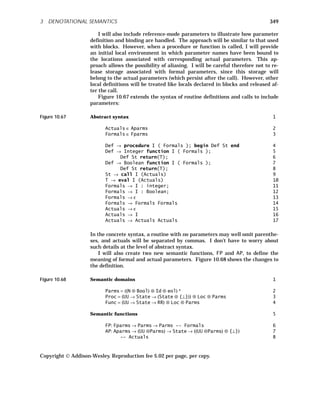
![FP[I: integer]p = append(p, << 0, I > , eol >) 9
FP[I: Boolean]p = append(p, << false, I > , eol >) 10
FP[ε]p = p 11
FP[Formals1 Formals2] p = FP[Formals2]q 12
where q = FP[Formals1]p. 13
AP[I] < u, p > s = v?Loc ∧ p≠eol ∧ 14
((Hd(pp)?N ∧ m(v)?N ⊕ {uninitInt}) ∨ (Hd(pp)?Bool ∧ 15
m(v)?Bool ⊕ {uninitBool})) ⇒ 16
< u[Hd[Tl(pp) ← v]], Tl(p) > , ⊥ 17
where v = Find(Tl(u))[I]; pp = Hd(p); s = < m, i, o > . 18
AP[ε] < u, p > s = < u, p > 19
AP[Actuals1 Actuals2] < u, p > s = q?{⊥} ⇒ ⊥, 20
AP[Actuals2] q s 21
where q = AP[Actuals1] < u, p > s. 22
D[procedure I (Formals); Def St] < u, s > = 23
Hd(u)[I]?{udef} ⇒ (l ?{⊥} ⇒ < u[Hd[I ← ⊥]], s > , 24
< uu, < m[l ← uninitInt], i, o >>), < u[Hd[I ← redef]], s > 25
where f(v, t) = S[St]v′t′; < v′, t′ > = D[Def] << v, uu > , t > ; 26
s = < m, i, o > ; l = alloc(m); 27
uu = u[Hd[I ←< f, l, p >]]; p = FP[Formals]eol. 28
D[Integer function(Formals) I; Def St return(T)] 29
< u, s > = Hd(u)[I]?{udef} ⇒ 30
(l ?{⊥} ⇒ < u[Hd[I ← ⊥]], s > , 31
< uu, < m[l ← uninitInt], i, o >>), < u[Hd[I ← redef]], s > 32
where s = < m, i, o > ; l = alloc(m); e(w, r) = E[T](w c(w, r)); 33
c(v, t) = S[St]v′t′; < v′, t′ > = D[Def] << v, uu > , t > ; 34
f(vv, tt) = c(vv, tt)?{⊥} ∨ e(vv, tt)?{⊥} ⇒ 35
⊥, (Tl(e(vv, tt))?N ⇒ e(vv, tt), ⊥); 36
uu = u[Hd[I ←< f, l, p >]]; p = FP[Formals]eol. 37
D[Boolean function(Formals) I; Def St return(T)] 38
< u, s > = Hd(u)[I]?{udef} ⇒ 39
(l ?{⊥} ⇒ < u[Hd[I ← ⊥]], s > , 40
< uu, < m[l ← uninitInt], i, o >>), < u[Hd[I ← redef]], s > 41
where s = < m, i, o > ; l = alloc(m); e(w, r) = E[T](w c(w, r)); 42
c(v, t) = S[St]v′t′; < v′, t′ > = D[Def] << v, uu > , t > ; 43
f(vv, tt) = c(vv, tt)?{⊥} ∨ e(vv, tt)?{⊥} ⇒ 44
⊥, (Tl(e(vv, tt))?Bool ⇒ e(vv, tt), ⊥); 45
uu = u[Hd[I ←< f, l, p >]]; p = FP[Formals]eol. 46
S[call I(Actuals)] u s = v?Proc ∧ 47
q≠⊥ ∧ Tl(q) = eol ⇒
i → ∞
lim pi(s, Hd(Hd(q))), ⊥ 48
where v = Find(u)[I] = < f, l, r > ; 49
p0(s′, u′) = ⊥; 50
pi+1(s′, u′) = m(l)?{uninitInt} ⇒ (w?{⊥} ⇒ ⊥, ww), 51
m(l) > 0 ∧ y?{⊥} ⇒ ⊥, yy; 52
q = AP[Actuals] << ue, u > , r > s; 53
s′ = < m, I, O > ; 54
w = f u′ < m[l ← i], I, O > ; 55
ww = w[Hd[l ← uninitInt]][Hd[Free(m) ← unalloc]]; 56
y = f u′ < m[l ← m(l) − 1], I, O > ; 57
yy = y[Hd[l ← m(l)]][Hd[Free(m) ← unalloc]]. 58
Copyright Addison-Wesley. Reproduction fee $.02 per page, per copy.
350 CHAPTER 10 FORMAL SYNTAX AND SEMANTICS](https://image.slidesharecdn.com/advancedprogramminglanguagedesign-230706034617-464d64c2/85/Advanced_programming_language_design-pdf-358-320.jpg)
![351
E[eval I(Actuals)] u s = v?Func ∧ q ≠ ⊥ ∧ Tl(q) = eol ⇒ 59
i → ∞
lim pi(s, Hd(Hd(q))), ⊥ 60
where v = Find(u)[I] = < f, l, r > ; 61
p0(s′, u′) = ⊥; 62
pi+1(s′, u′) = m(l)?{uninitInt} ⇒ (w?{⊥} ⇒ ⊥, ww), 63
m(l) > 0 ∧ y?{⊥} ⇒ ⊥, yy; 64
q = AP[Actuals] << ue, u > , r > s; 65
s′ = < m, I, O > ; 66
w = f u′ < m[l ← i], I, O > ; 67
ww = w[Hd[l ← uninitInt]][Hd[Free(m) ← unalloc]]; 68
y = f u′ < m[l ← m(l) − 1], I, O > ; 69
yy = y[Hd[l ← m(l)]][Hd[Hd[Free(m) ← unalloc]]]. 70
The eol in line 2 represents “end of list.”
3.19 Continuations
The denotational approach is very structured; the meaning of a construct is
defined in terms of a composition of the meanings of the construct’s con-
stituents. The meaning of a program can be viewed as a top-down traversal
of an abstract syntax tree from the root (the program nonterminal) to the
leaves (identifiers, constants, and so forth). The meanings associated with
the leaves are then percolated back up to the root, where the meaning of the
whole program is determined.
This structured approach has problems with statements such as break or
goto that don’t readily fit the composition model. Further, it forces values to
percolate throughout the whole tree, even if this action is unnecessary. Con-
sider, for example, a stop statement. When stop is executed, I would like to
discontinue statement evaluation and immediately return to the main pro-
gram production, where the final result (the output file) is produced. But I
can’t; the meaning of stop must be composed with that of the remaining
statements (even though stop means one must ignore the remaining state-
ments!). As it stands, my definition of the meaning of a statement sequence
(see lines 90–91 in Figure 10.62, page 345) checks for error on the first state-
ment before evaluating the second. I could add another sort of value, like ⊥,
that indicates that execution should stop, even though there is no error. This
device would work but would be rather clumsy, as I would model stop not by
stopping but by continuing to traverse program statements while ignoring
them.
Continuations were invented to remedy these problems. A continuation
is a function passed as a parameter to every semantic function. The semantic
function determines its value as usual and then calls (directly or indirectly)
the continuation with its value as a parameter. This approach is quite clever
but is much less intuitive than the structured approach I have presented so
far.
I will first consider expression continuations, which have a semantic do-
main EC, defined as:
EC = (N ⊕ Bool) → State → R
The expression continuation takes a value and a state (since side effects in
Copyright Addison-Wesley. Reproduction fee $.02 per page, per copy.
3 DENOTATIONAL SEMANTICS](https://image.slidesharecdn.com/advancedprogramminglanguagedesign-230706034617-464d64c2/85/Advanced_programming_language_design-pdf-359-320.jpg)
![evaluating the expression can change the state) and produces a result. The E
semantic function will now include an expression continuation as a parame-
ter:
E: Exp → UU → State → EC → R
E now produces a result rather than a state-result pair because state changes
are included in the continuation component. Figure 10.69 now redefines the
meaning of simple integer-valued bit strings. The expression continuation, k,
uses the value and state computed by the semantic function E.
Figure 10.69 Semantic functions 1
E[0] u s k = k(0, s) 2
E[1] u s k = k(1, s) 3
E[Seq 0] u s k = E[Seq] u s k1 4
where k1(r, t) = range(2 × r)?{⊥} ⇒ ⊥, k(2 × r, t). 5
E[Seq 1] u s k = E[Seq] u s k1 6
where k1(r, t) = range(2 × r + 1)?{⊥} ⇒ ⊥, k(2 × r + 1, t). 7
It is no longer necessary to test if a construct produces ⊥; if it does, the
construct returns ⊥ immediately. Otherwise, it calls its continuation parame-
ter with values it knows to be valid. To see how evaluation proceeds, consider
the following example. Evaluate E[111]ue s0 K, where ue and s0 are the empty
environment and initial state, and K(r,s)=r returns the final result.
1. E[111]ue s0 K = E[11]ue s0 k1, where
k1(r1, s1) = range(2 × r1 + 1)?{⊥} ⇒ ⊥, K(2 × r1 + 1, s1).
2. E[11]ue s0 k1 = E[1]ue s0 k2, where
k2(r2, s2) = range(2 × r2 + 1)?{⊥} ⇒ ⊥, k1(2 × r2 + 1, s2).
3. E[1]ue s0 k2 = k2(1, s0) = range(2 × 1 + 1)?{⊥} ⇒ ⊥, k1(2 × 1 + 1, s0) =
k1(3, s0) = range(2 × 3 + 1)?{⊥} ⇒ ⊥, K(2 × 3 + 1, s0) = K(7, s0) = 7.
Figure 10.70 shows how the binary operators are handled.
Figure 10.70 Semantic functions 1
E[T1 + T2] u s k = E[T1] u s k1 2
where k1(r1, s1) = r1?N ⇒ E[T2] u s1 k2, ⊥; 3
k2(r2, s2) = r2?N ∧ range(r1 + r2)?N ⇒ k(r1 + r2, s2), ⊥. 4
Consider this example: Compute E[22 + 33]ue s0 K, where again K(r, s) = r.
1. E[22 + 33]ue s0 K = E[22]ue s0 k1, where
k1(r1, s1) = r1?N ⇒ E[33] u s1 k2, k2(r2, s2) = r2?N and
range(r1 + r2)?N ⇒ k(r1 + r2, s2), ⊥.
2. E[22]ue s0 k1 = k1(22, s0) = 22?N ⇒ E[33]ue s0 k2, ⊥ =
E[33]ue s0 k2 = k2(33, s0) = 33?N and
range(22 + 33)?N ⇒ K(22 + 33, s0), ⊥ = K(55, s0) = 55.
The rest of the binary operators are similar in form, as shown in Figure
10.71.
Copyright Addison-Wesley. Reproduction fee $.02 per page, per copy.
352 CHAPTER 10 FORMAL SYNTAX AND SEMANTICS](https://image.slidesharecdn.com/advancedprogramminglanguagedesign-230706034617-464d64c2/85/Advanced_programming_language_design-pdf-360-320.jpg)
![353
Figure 10.71 Semantic functions 1
E[T1 − T2] u s k = E[T1] u s k1 2
where k1(r1, s1) = r1?N ⇒ E[T2] u s1 k2, ⊥; 3
k2(r2, s2) = r2?N ∧ range(r1 − r2)?N ⇒ k(r1 − r2, s2), ⊥. 4
E[T1 * T2] u s k = E[T1] u s k1 5
where k1(r1, s1) = r1?N ⇒ E[T2] u s1 k2, ⊥; 6
k2(r2, s2) = r2?N ∧ range(r1 × r2)?N ⇒ k(r1 × r2, s2), ⊥. 7
E[T1/T2] u s k = E[T1] u s k1 8
where k1(r1, s1) = r1?N ⇒ E[T2] u s1 k2, ⊥; 9
k2(r2, s2) = r2?N ∧ r2≠0 ∧ range(r1/r2)?N ⇒ k(r1/r2, s2), ⊥. 10
E[T1 = T2] u s k = E[T1] u s k1 11
where k1(r1,s1) = E[T2] u s1 k2; 12
k2(r2, s2) = (r1?N ∧ r2?N) ∨ (r1?Bool ∧ r2?Bool) ⇒ 13
k(r1 = r2, s2), ⊥. 14
Identifier lookup is straightforward; see Figure 10.72.
Figure 10.72 E[I] u s k = v?({⊥} ⊕ {redef} ⊕ {udef}) ⇒ ⊥, 1
v?Loc ⇒ (m(v)?({uninitInt}⊕{uninitBool}) ⇒ 2
⊥, k(m(v), s)), k(v, s) 3
where v = Find(u)[I]; s = < m, i, o > . 4
To see how side effects are handled, I will introduce an assignment expression
similar to that found in C: I ← T is an expression that evaluates to T and (as a
side effect) sets I to T, as in Figure 10.73.
Figure 10.73 E[I ← T] u s k = E[T] u s k1 1
where k1(r, t) = v?Loc ∧ 2
((r?N ∧ m(v)?N ⊕ {uninitInt}) ∨ 3
(r?Bool ∧ m(v)?Bool ⊕ {uninitBool})) ⇒ 4
k(r, < m[v ← r], i, o >), ⊥. 5
t = < m, i, o > ; v = Find(u)[I]. 6
Consider this example: Compute E[I + I ← 0]u0 s0 K, where u0 and s0 contain a
variable I with value 10 and K(r, s) = r + Hd(s)(u0[I]) adds the final value of I to
the value of the expression.
1. E[I + I ← 0]u0 s0 K = E[I]u0 s0 k1, where
k1(r1, s1) = r1?N ⇒ E[I ← 0] u s1 k2, ⊥. k2(r2, s2) = r2?N.
range(r1 + r2)?N ⇒ K(r1 + r2, s2), ⊥.
2. E[I]u0 s0 k1 = v?({⊥} ⊕ {redef} ⊕ {udef}) ⇒ ⊥.
v?Loc ⇒(m(v)?({uninitInt}⊕{uninitBool}) ⇒ ⊥, k1(m(v), s0)), k1(v, s0),
where v = Find(u0)[I], s0 = < m, i, o >.
3. E[I]u0 s0 k1 = k1(m(v), s0) = k1(10, s0) = 10?N ⇒
E[I ← 0] u s0 k2, ⊥ = E[I ← 0] u s0 k2.
4. E[I ← 0]u0 s0 k2 = E[0]u0 s0 k3, where
k3(r, t) = v?Loc ∧ ((r?N ∧ m(v)?N ⊕ {uninitInt}) ∨
(r?Bool ∧ m(v)?Bool⊕{uninitBool})) ⇒ k2(r, < m[v ← r], i, o >), ⊥.
t = < m, i, o > , v = Find(u)[I].
Copyright Addison-Wesley. Reproduction fee $.02 per page, per copy.
3 DENOTATIONAL SEMANTICS](https://image.slidesharecdn.com/advancedprogramminglanguagedesign-230706034617-464d64c2/85/Advanced_programming_language_design-pdf-361-320.jpg)
![5. E[0] u s0 k3 = k3(0, s0) = v?Loc ∧ ((0?N ∧ m(v)?N ⊕{uninitInt}) ∨
(0?Bool ∧ m(v)?Bool⊕{uninitBool})) ⇒ k2(0, < m[v ← 0], i, o >), ⊥.
s0 = < m, i, o > . v = Find(u)[I].
6. E[0] u s0 k3 = k2(0, < m[v ← 0], i, o >) = k2(0, ss0), where
ss0 = < m[v ← 0], i, o > . k2(0, ss0) = 0?N.
range(10 + 0)?N ⇒ K(0 + 10, ss0), ⊥ = K(0 + 10, ss0).
7. K(10, ss0) = 10 + Hd(ss0)(u0[I]) = 10 + 0 = 10.
Continuations execute in the state that is current when they are evalu-
ated, not in the state that is current when they are defined (that’s why they
take state as a parameter).
3.20 Statement Continuations
I am now ready to consider statement continuations, which are particularly
useful because they allow me to handle nonstructured control flows. I will
first define SC, the semantic domain of statement continuations (see Figure
10.74). I will also slightly alter EC, the semantic domain of expression contin-
uations. In both cases, the continuations will return Ans, the domain of pro-
gram answers, reflecting the fact that expressions and statements are not
executed in isolation, but rather in contexts in which they contribute to the fi-
nal answer to be computed by the whole program.
Figure 10.74 Semantic domains 1
Ans = File ⊕ {⊥} 2
EC = (N ⊕ Bool) → State → Ans 3
SC = State → Ans 4
Statement continuations take only one parameter because the only program
component updated by a statement is the state. Figure 10.75 extends the S
semantic function to include a statement continuation parameter. All seman-
tic functions now return Ans because they all execute by evaluating (directly
or indirectly) some continuation function. The values that change during the
computation of a semantic function (a result, environment, or state) are now
parameters to a continuation function.
Figure 10.75 Semantic functions 1
E: Exp → UU → State → EC → Ans 2
S: Stm → UU → State → SC → Ans 3
To see the utility of statement continuations, consider the definition of state-
ment composition in Figure 10.76.
Figure 10.76 S[St1 St2] u s c = S[St1] u s c′ 1
where c′(s′) = S[St2] u s′c. 2
The statement continuation has a fairly intuitive interpretation: what to exe-
cute after the current statement. The advantage of the continuation ap-
Copyright Addison-Wesley. Reproduction fee $.02 per page, per copy.
354 CHAPTER 10 FORMAL SYNTAX AND SEMANTICS](https://image.slidesharecdn.com/advancedprogramminglanguagedesign-230706034617-464d64c2/85/Advanced_programming_language_design-pdf-362-320.jpg)
![355
proach is now evident. A statement need not execute its continuation if an
abnormal transfer of control is indicated. A stop statement executes by re-
turning an answer (the current value of the output file). Similarly, goto exe-
cutes by looking up (and executing) a statement continuation stored in the
environment as the value of the label!
I can now consider other statements, as shown in Figure 10.77.
Figure 10.77 S[ε] u s c = c(s) 1
S[I: = T] u s c = E[T] u s k 2
where k(r, t) = v?Loc ∧ 3
((r?N ∧ m(v)?N ⊕ {uninitInt}) ∨ 4
(r?Bool ∧ m(v)?Bool ⊕ uninitBool)) ⇒ 5
c(< m[v ← r], i, o >), ⊥; 6
t = < m, i, o > ; v = Find(u)[I]. 7
S[read I] u s c = v?Loc ∧ i ≠ eof ∧ 8
((Hd(i)?N ∧ m(v)?N ⊕ uninitInt) ∨ 9
(Hd(i)?Bool ∧ m(v)?Bool ⊕ uninitBool)) ⇒ 10
c(< m[v ← Hd(i)], Tl(i), o >), ⊥ 11
where s = < m, i, o > ; v = Find(u)[I]. 12
S[write T] u s c = E[T] u s k 13
where k(r, t) = c(< m, i, append(o, < r, eof >) >); t = < m, i, o > . 14
S[if T then St1 else St2] u s c = 15
E[T] u s k 16
where k(r, t) = r?Bool ⇒ (r ⇒ S[St1] u t c, S[St2] u t c), ⊥. 17
S[do T times St] u s c = E[T] u s k 18
where k(r, t) = r?N ⇒ vm(t), ⊥; 19
m = max(0, r); v0(s′) = c(s′); vi+1(s′) = S[St] u s′vi. 20
S[while T do St] u s c =
i → ∞
lim pi(s) 21
where p0(s′) = ⊥; pi+1(s′) = E[T] u s′ ki+1; 22
ki+1(r, t) = r?Bool ⇒ (r ⇒ S[St] u t pi, c(t)), ⊥ 23
3.21 Declaration Continuations
A declaration continuation will map an environment and state into an an-
swer. The D function will now take a declaration continuation from the do-
main DC, as in Figure 10.78.
Figure 10.78 DC = UU → State → Ans 1
D: Decls → UU → State → DC → Ans 2
Copyright Addison-Wesley. Reproduction fee $.02 per page, per copy.
3 DENOTATIONAL SEMANTICS](https://image.slidesharecdn.com/advancedprogramminglanguagedesign-230706034617-464d64c2/85/Advanced_programming_language_design-pdf-363-320.jpg)
![D[I: integer] u s d = Hd(u)[I]?{udef} ⇒ 3
(l ?{⊥} ⇒ d(u[Hd[I ← ⊥]], s), 4
d(u[Hd[I ← l]], < m[l ← uninitInt], i, o >)), 5
d(u[Hd[I ← redef]], s) 6
where s = < m, i, o > ; l = alloc(m). 7
D[I: Boolean] u s d = Hd(u)[I]?{udef} ⇒ 8
(l ?{⊥} ⇒ d(u[Hd[I ← ⊥]], s), 9
d(u[Hd[I ← l]], < m[l ← uninitBool], i, o >)), 10
d(u[Hd[I ← redef]], s) 11
where s = < m, i, o > ; l = alloc(m). 12
D[I = T] u s d = E[T] u s k 13
where k(r, t) = Hd(u)[I]?{udef} ⇒ 14
d(u[Hd[I ← r]], t), d(u[Hd[I ← redef]], t). 15
The expression T (line 13) can be allowed to contain function calls. If evalua-
tion of T faults, E will simply return ⊥; otherwise, it executes the declaration
continuation (d) with the value that T returns and a possibly updated state.
Other definitions are given in Figure 10.79.
Figure 10.79 D[ε] u s d = d(u, s) 1
D[Def1 Def2] u s d = D[Def1] u s d′ 2
where d′(v, t) = D[Def2] v t d. 3
S[begin Def St end] u s c = D[Def] < ue, u > s d 4
where d(v, t) = S[St] v t c′; 5
c′(t′) = c(t′[Hd[Free(Hd(s)) ← unalloc]]). 6
3.22 Procedures, Functions, and
Parameters
I now define routines and parameters in the new continuation notation.
First, declarations need to be handled, using D, DC, FP, and FC (formal param-
eter continuation), as shown in Figure 10.80.
Figure 10.80 FC = Parms → Ans 1
FP: Fparms → Parms → FC → Ans 2
FP[I : integer] p f = f(append(p, << 0, I > , eol >)) 3
FP[I : Boolean] p f = f(append(p, << false, I > , eol >)) 4
FP[ε] p f = f(p) 5
FP[Formals1 Formals2] p f = FP[Formals1] p f′ 6
where f′(p′) = FP[Formals2]p′f. 7
Procedures are generalizations of statements, and, like all statements, take a
statement continuation as a parameter. This continuation is essentially the
return point of the procedure; see Figure 10.81.
Copyright Addison-Wesley. Reproduction fee $.02 per page, per copy.
356 CHAPTER 10 FORMAL SYNTAX AND SEMANTICS](https://image.slidesharecdn.com/advancedprogramminglanguagedesign-230706034617-464d64c2/85/Advanced_programming_language_design-pdf-364-320.jpg)
![357
Figure 10.81 Proc = (U → State → SC → Ans) ⊗ Loc ⊗ Parms 1
D[procedure I (Formals); Def St] u s d = 2
FP[Formals]eol f, 3
where f(p) = Hd(u)[I]?{udef} ⇒ 4
(l ?{⊥} ⇒ d(u[Hd[I ← ⊥]], s), 5
d(uu, < m[l ← uninitInt], i, o >)), 6
d(u[Hd[I ← redef]], s); 7
s = < m, i, o > ; l = alloc(m); uu = u[Hd[I ←< r, l, p >]]; 8
r(v, t, cc) = D[Def] < v, uu > t d′; 9
d′(v′, t′) = S[St]v′t′c′; 10
c′(tt) = cc(tt[Hd[Free(t) ← unalloc]]). 11
Since functions are a generalization of expressions, they will now include an
expression continuation that represents the mechanism through which the
function’s value is returned, as in Figure 10.82.
Figure 10.82 Func = (U → State → EC → Ans) ⊗ Loc ⊗ Parms 1
D[Integer function(Formals) I; St; return(T)] u s d = 2
FP[Formals]eol f, 3
where f(p) = Hd(u)[I]?{udef} ⇒ 4
(l ?{⊥} ⇒ d(u[Hd[I ← ⊥]], s), 5
d(uu, < m[l ← uninitInt], i, o >)), 6
d(u[Hd[I ← redef]], s); 7
s = < m, i, o > ; l = alloc(m); uu = u[Hd[I ←< r, l, p >]]; 8
r(u′, s′, ec) = D[Def] < u′, uu > s′d′; 9
d′(v, t) = S[St] v t c; 10
c(v′, t′) = E[T]v′t′k; 11
k(r, tt) = r?N ⇒ ec(r, tt[Hd[Free(s′) ← unalloc]]), ⊥. 12
D[Boolean function(Formals) I; St; return(T)] u s d = 13
FP[Formals]eol f, 14
where f(p) = Hd(u)[I]?{udef} ⇒ 15
(l ?{⊥} ⇒ d(u[Hd[I ← ⊥]], s), 16
d(uu, < m[l ← uninitInt], i, o >)), 17
d(u[Hd[I ← redef]], s); 18
s = < m, i, o > ; l = alloc(m); uu = u[Hd[I ←< r, l, p >]]; 19
r(u′, s′, ec) = D[Def] < u′, uu > s′ d′; 20
d′(v, t) = S[St] v t c; 21
c(v′, t′) = E[T]v′ t′ k; 22
k(r, tt) = r?Bool ⇒ ec(r, tt[Hd[Free(s′) ← unalloc]]), ⊥. 23
Copyright Addison-Wesley. Reproduction fee $.02 per page, per copy.
3 DENOTATIONAL SEMANTICS](https://image.slidesharecdn.com/advancedprogramminglanguagedesign-230706034617-464d64c2/85/Advanced_programming_language_design-pdf-365-320.jpg)
![It is time to consider actual-parameter evaluation and procedure and function
calls; see Figure 10.83. AC is the semantic domain of actual-parameter contin-
uations.
Figure 10.83 AC = UU → Parms → Ans 1
AP: Aparms → UU → Parms → State → AC → Ans 2
AP[I] u p s a = v?Loc ∧ p ≠ eol ∧ 3
((Hd(pp)?N ∧ m(v)?N ⊕ uninitInt) ∨ 4
(Hd(pp)?Bool ∧ m(v)?Bool ⊕ uninitBool)) ⇒ 5
a(u[Hd[Tl(pp) ← v]], Tl(p)), ⊥ 6
where v = Find(Tl(u))[I]; pp = Hd(p); s = < m, i, o > . 7
AP[ε] u p s a = a(u, p) 8
AP[Actuals1 Actuals2] u p s a = 9
AP[Actuals1] u p s a′ 10
where a′(u′, p′) = AP[Actuals2]u′ p′ s a. 11
S[call I(Actuals)] u s c = v?Proc ⇒ 12
AP[Actuals] < ue, u > r sa, ⊥ 13
where a(u′, q) = (q = eol) ⇒ 14
i → ∞
lim pi(s, Hd(u′)), ⊥; 15
v = Find(u)[I] = < f, l, r > ; 16
p0(s′, w) = ⊥; 17
pi+1(s′, w) = m(l) = uninitInt ⇒ 18
f w < m[l ← i], I, O > c1, 19
m(l) > 0 ⇒ f w < m[l ← m(l) − 1], I, O > c2, ⊥; 20
s′ =< m, I, O > ; 21
c1(t1) = c(t1[Hd[l <- uninitInt]]); 22
c2(t2) = c(t2[Hd[l <- m(l)]]). 23
E[eval I (Actuals)] u s k = v?Func ⇒ 24
AP[Actuals] < ue, u > r sa, ⊥ 25
where a(u′, q) = (q = eol) ⇒ 26
i → ∞
lim pi(s, Hd(u′)), ⊥; 27
v = Find(u)[I] = < f, l, r > ; 28
p0(s′, w) = ⊥; 29
pi+1(s′, w) = m(l) = uninitInt ⇒ 30
f w < m[l ← i], I, O > k1, 31
m(l) > 0 ⇒ f w < m[l ← m(l) − 1], I, O > k2, ⊥; 32
s′ = < m, I, O > ; 33
k1(r1, t1) = k(r1, t1[Hd[l ← uninitInt]]); 34
k2(r2, t2) = k(r1, t2[Hd[l ← m(l)]]). 35
Finally, I redefine the M function using continuations, as shown in Figure
10.84.
Copyright Addison-Wesley. Reproduction fee $.02 per page, per copy.
358 CHAPTER 10 FORMAL SYNTAX AND SEMANTICS](https://image.slidesharecdn.com/advancedprogramminglanguagedesign-230706034617-464d64c2/85/Advanced_programming_language_design-pdf-366-320.jpg)
![359
Figure 10.84 M: Pr → File → Ans 1
M[program Def St end] i = 2
D[Def] < ue, u0 > < m0, i, eof > d 3
where d(v, t) = S[St] v tc; c(t′) = Tl(Tl(t′)). 4
3.23 Flow of Control
Now that I have the machinery of continuations in place, I can illustrate how
to implement statements that alter the flow of control. I begin with the stop
statement, which forces immediate termination of execution. Figure 10.85
shows the semantic function.
Figure 10.85 S[stop] u s c = Tl(Tl(s))
Stop returns the output file component of the current state. It avoids the nor-
mal flow of control by ignoring its continuation parameter.
A more interesting illustration is break, which I will use to exit any of the
structured statements in the language (if, do, while, begin-end). I will let
any of these statements be optionally labeled with an identifier, which will
follow normal scoping rules. I define break I to cause execution to immedi-
ately break out of the structure labeled with I and then to continue execution
with the normal successor to the labeled statement. If I isn’t declared as a la-
bel in the scope of the break, the statement produces an error value.
I extend V, the domain of environment contents, to include statement con-
tinuations:
U = Id → V
V = N ⊕ Bool ⊕ Loc ⊕ Proc ⊕ Func ⊕ SC ⊕ {⊥}⊕{udef}⊕{redef}
The meaning of a label on a structured statement will be the continuation as-
sociated with that statement. Figure 10.86 adds definitions for structured
statements with labels (the definitions for unlabeled statements are, of
course, retained).
Figure 10.86 S[I: if T thenSt1 else St2] u s c = E[T] uu s k 1
where k(r, t) = r?Bool ⇒ (r ⇒ S[St1] uu t c, S[St2] uu t c), ⊥; 2
uu = Hd(u)[I]?{udef} ⇒ u[Hd[I ← c′]], u[Hd[I ← redef]]; 3
c′(t′) = c(t′[Hd[Free(Hd(s)) ← unalloc]]). 4
S[I: do T times St] u s c = E[T] uu s k 5
where k(r, t) = r?N ⇒ vm(t), ⊥; 6
m = max(0, t); v0(s′) = c(s′); 7
vi+1(s′) = S[St] uu s′ vi; 8
uu = Hd(u)[I]?{udef} ⇒ u[Hd[I ← c′]], u[Hd[I ← redef]]; 9
c′(t′) = c(t′[Hd[Free(Hd(s)) ← unalloc]]). 10
S[I: while T do St] u s c =
i → ∞
lim pi(s) 11
where p0(s′) = ⊥; pi+1(s′) = E[T] uu s′ ki+1; 12
ki+1(r, t) = r?Bool ⇒ (r ⇒ S[St] uu t pi, c(t)), ⊥; 13
uu = Hd(u)[I]?{udef} ⇒ u[Hd[I ← c′]], u[Hd[I ← redef]]; 14
c′(t′) = c(t′[Hd[Free(Hd(s)) ← unalloc]]); 15
Copyright Addison-Wesley. Reproduction fee $.02 per page, per copy.
3 DENOTATIONAL SEMANTICS](https://image.slidesharecdn.com/advancedprogramminglanguagedesign-230706034617-464d64c2/85/Advanced_programming_language_design-pdf-367-320.jpg)
![S[I: begin Def St end] u s c = 16
D[Def] < ue, uu > s d, 17
where d(v, t) = S[St] v t c′; 18
c′(t′) = c(t′[Hd[Free(Hd(s)) ← unalloc]]); 19
uu = Hd(u)[I]?{udef} ⇒ u[Hd[I ← c′]], u[Hd[I ← redef]]. 20
Break looks up its identifier, and if it is bound to a statement continuation, it
executes that continuation in the current state; see Figure 10.87.
Figure 10.87 S[break I] u s c = v?SC ⇒ v(s), ⊥ 1
where v = Find(u)[I]. 2
3.24 Summary of Syntactic and Semantic
Domains and Semantic Functions
The domains used in the denotational definitions in this chapter have been
upgraded during the progression of examples. Figure 10.88 lists the most re-
cent meanings.
Figure 10.88 Syntactic domains 1
BinLit: binary literals; nonterminals BN, Seq 2
Exp: expressions; nonterminal T 3
Id: identifiers; nonterminal I 4
Pr: programs; nonterminal P 5
Decls: declarations; nonterminal Def 6
Stm: statements; nonterminal St 7
Semantic domains 8
Basic: 9
N = {0, 1, 2, ...} (natural numbers) 10
Bool = {false, true} (Boolean values) 11
Complex: 12
Loc = {0, 1, . . . } -- finite domain of memory locations 13
Mem = Loc → N ⊕ Bool ⊕ {uninitInt} ⊕ {uninitBool} ⊕ 14
{unalloc} -- memory location 15
File = (N ⊕ Bool ⊕ {eof}) * -- contents of a file 16
R = N ⊕ Bool ⊕ {⊥} -- value of an expression 17
RR = State ⊗ (N ⊕ Bool ⊕ {⊥}) 18
-- result of function 19
State = Mem ⊗ File ⊗ File -- program state 20
Ans = File ⊕ {⊥} -- program result 21
V = N ⊕ Bool ⊕ Loc ⊕ Proc ⊕ Func ⊕ SC ⊕ {⊥} ⊕ {udef} ⊕ 22
{redef} -- value of an identifier 23
U = Id → V -- environment 24
UU = U * -- sequence of environments 25
Proc = (U → State → SC → Ans) ⊗ Loc ⊗ Parms 26
-- procedure 27
Func = (U → State → EC → Ans) ⊗ Loc ⊗ Parms 28
-- function 29
Copyright Addison-Wesley. Reproduction fee $.02 per page, per copy.
360 CHAPTER 10 FORMAL SYNTAX AND SEMANTICS](https://image.slidesharecdn.com/advancedprogramminglanguagedesign-230706034617-464d64c2/85/Advanced_programming_language_design-pdf-368-320.jpg)
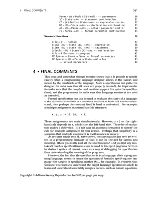
![There is no guarantee that every error case has been dealt with, and the no-
tation is complex enough that such an omission would probably pass unno-
ticed.
The fact that I have succeeded in denoting standard features of a pro-
gramming language gives me no particular confidence that I could handle
such constructs as CLU coroutines (Chapter 2), ML higher-level functions
(Chapter 3), Prolog resolution (Chapter 8), Post guardians (Chapter 6),
SNOBOL patterns (Chapter 9), or Modula monitors (Chapter 7). An enor-
mous amount of cleverness is required to build denotational semantic defini-
tions. As you have seen, introducing a single concept into a language is likely
to modify the definitions for everything else. A typical modification involves
making functions like E even higher-order. The result is anything but
straightforward.
Several excellent books deal with programming language semantics. I can
especially recommend Tennent [Tennent 81] and Pagan [Pagan 81].
EXERCISES
Review Exercises
10.1 Describe the language (that is, the set of strings) generated by this BNF
grammar:
S ::= ( S ) S | ε
10.2 Show a different BNF grammar that generates exactly the same lan-
guage as the grammar in Exercise 10.1.
10.3 Write BNF productions for if statements.
10.4 An ambiguous grammar is one that generates strings that have more
than one parse tree. Is the grammar of Figure 10.89 ambiguous? Does
it have any other problems?
Figure 10.89 Expression ::= 1
Expression + Expression | 2
Expression * Expression | 3
INTEGER 4
10.5 Prove the program in Figure 10.90 correct.
Figure 10.90 {a < 3} 1
if a < 4 then x := 2 else x := 10 end; 2
{x = 2} 3
Copyright Addison-Wesley. Reproduction fee $.02 per page, per copy.
362 CHAPTER 10 FORMAL SYNTAX AND SEMANTICS](https://image.slidesharecdn.com/advancedprogramminglanguagedesign-230706034617-464d64c2/85/Advanced_programming_language_design-pdf-370-320.jpg)