This document presents a machine learning methodology for diagnosing chronic kidney disease (CKD) utilizing a dataset from the UCI Machine Learning Repository, which was processed to handle missing values using k-nearest neighbor (KNN) imputation. Six machine learning algorithms were employed, with Random Forest yielding a diagnosis accuracy of 99.75%, while an integrated model combining Logistic Regression and Random Forest achieved an average accuracy of 99.83%. The findings suggest that this methodology could enhance early detection and timely treatment of CKD in clinical settings.

1. Received December 5, 2019, accepted December 16, 2019, date of publication December 30, 2019, date of current version February 4, 2020.
Digital Object Identifier 10.1109/ACCESS.2019.2963053
A Machine Learning Methodology for
Diagnosing Chronic Kidney Disease
JIONGMING QIN 1, LIN CHEN 2, YUHUA LIU 1, CHUANJUN LIU 2,
CHANGHAO FENG 1, AND BIN CHEN 1
1Chongqing Key Laboratory of Non-linear Circuit and Intelligent Information Processing, College of Electronic and Information Engineering, Southwest
University, Chongqing 400715, China
2Department of Electronics, Graduate School of Information Science and Electrical Engineering, Kyushu University, Fukuoka 819-0395, Japan
Corresponding author: Bin Chen (chenbin121@swu.edu.cn)
This work was supported in part by the National Nature Science Foundation of China under Grant 61801400 and Grant 61703348, and in
part by the Central Universities under Grant XDJK2018C021, Grant JSPS KAKENHI, and Grant JP18F18392.
ABSTRACT Chronic kidney disease (CKD) is a global health problem with high morbidity and mortality
rate, and it induces other diseases. Since there are no obvious symptoms during the early stages of CKD,
patients often fail to notice the disease. Early detection of CKD enables patients to receive timely treatment
to ameliorate the progression of this disease. Machine learning models can effectively aid clinicians achieve
this goal due to their fast and accurate recognition performance. In this study, we propose a machine
learning methodology for diagnosing CKD. The CKD data set was obtained from the University of California
Irvine (UCI) machine learning repository, which has a large number of missing values. KNN imputation was
used to fill in the missing values, which selects several complete samples with the most similar measurements
to process the missing data for each incomplete sample. Missing values are usually seen in real-life medical
situations because patients may miss some measurements for various reasons. After effectively filling out
the incomplete data set, six machine learning algorithms (logistic regression, random forest, support vector
machine, k-nearest neighbor, naive Bayes classifier and feed forward neural network) were used to establish
models. Among these machine learning models, random forest achieved the best performance with 99.75%
diagnosis accuracy. By analyzing the misjudgments generated by the established models, we proposed an
integrated model that combines logistic regression and random forest by using perceptron, which could
achieve an average accuracy of 99.83% after ten times of simulation. Hence, we speculated that this
methodology could be applicable to more complicated clinical data for disease diagnosis.
INDEX TERMS Chronic kidney disease, machine learning, KNN imputation, integrated model.
I. INTRODUCTION
Chronic kidney disease (CKD) is a global public health prob-
lem affecting approximately 10% of the world’s population
[1], [2]. The percentage of prevalence of CKD in China is
10.8% [3], and the range of prevalence is 10%-15% in the
United States [4]. According to another study, this percentage
has reached 14.7% in the Mexican adult general population
[5]. This disease is characterised by a slow deterioration in
renal function, which eventually causes a complete loss of
renal function. CKD does not show obvious symptoms in its
early stages. Therefore, the disease may not be detected until
the kidney loses about 25% of its function [6]. In addition,
CKD has high morbidity and mortality, with a global impact
The associate editor coordinating the review of this manuscript and
approving it for publication was Hao Ji.
on the human body [7]. It can induce the occurrence of
cardiovascular disease [8], [9]. CKD is a progressive and
irreversible pathologic syndrome [10]. Hence, the prediction
and diagnosis of CKD in its early stages is quite essential,
it may be able to enable patients to receive timely treatment
to ameliorate the progression of the disease.
Machine learning refers to a computer program, which
calculates and deduces the information related to the task
and obtains the characteristics of the corresponding pattern
[11]. This technology can achieve accurate and economical
diagnoses of diseases; hence, it might be a promising method
for diagnosing CKD. It has become a new kind of medical
tool with the development of information technology [12]
and has a broad application prospect because of the rapid
development of electronic health record [13]. In the medical
field, machine learning has already been used to detect human
VOLUME 8, 2020
This work is licensed under a Creative Commons Attribution 4.0 License. For more information, see http://creativecommons.org/licenses/by/4.0/
20991

2. J. Qin et al.: Machine Learning Methodology for Diagnosing CKD
body status [14], analyze the relevant factors of the disease
[15] and diagnose various diseases. For example, the models
built by machine learning algorithms were used to diagnose
heart disease [16], [17], diabetes and retinopathy [18], [19],
acute kidney injury [20], [21], cancer [22] and other diseases
[23], [24]. In these models, algorithms based on regression,
tree, probability, decision surface and neural network were
often effective. In the field of CKD diagnosis, Hodneland
et al. utilized image registration to detect renal morphologic
changes [25]. Vasquez-Morales et al. established a classifier
based on neural network using large-scale CKD data, and
the accuracy of the model on their test data was 95% [26].
In addition, most of the previous studies utilized the CKD
data set that was obtained from the UCI machine learning
repository. Chen et al. used k-nearest neighbor (KNN), sup-
port vector machine (SVM) and soft independent modelling
of class analogy to diagnose CKD, KNN and SVM achieved
the highest accuracy of 99.7% [27]. In addition, they used
fuzzy rule-building expert system, fuzzy optimal associative
memory and partial least squares discriminant analysis to
diagnose CKD, and the range of accuracy in those models was
95.5%-99.6% [1]. Their studies have achieved good results
in the diagnosis of CKD. In the above models, the mean
imputation is used to fill in the missing values and it depends
on the diagnostic categories of the samples. As a result,
their method could not be used when the diagnostic results
of the samples are unknown. In reality, patients might miss
some measurements for various reasons before diagnosing.
In addition, for missing values in categorical variables, data
obtained using mean imputation might have a large deviation
from the actual values. For example, for variables with only
two categories, we set the categories to 0 and 1, but the
mean of the variables might be between 0 and 1. Polat et al.
developed an SVM based on feature selection technology,
the proposed models reduced the computational cost through
feature selection, and the range of accuracy in those models
was from 97.75%-98.5% [6]. J. Aljaaf et al. used novel mul-
tiple imputation to fill in the missing values, and then MLP
neural network (MLP) achieved an accuracy of 98.1% [28].
Subas et al. used MLP, SVM, KNN, C4.5 decision tree and
random forest (RF) to diagnose CKD, and the RF achieved an
accuracy of 100% [2]. In the models established by Boukenze
et al., MLP achieved the highest accuracy of 99.75% [29].
The studies of [2], [29] focus mainly on the establishment
of models and achieve an ideal result. However, a complete
process of filling in the missing values is not described in
detail, and no feature selection technology is used to select
predictors as well. Almansour et al. used SVM and neural
network to diagnose CKD, and the accuracy of the models
was 97.75% and 99.75%, respectively [30]. In the models
established by Gunarathne et al., zero was used to fill out the
missing values and decision forest achieved the best perfor-
mance with the accuracy was 99.1% [31].
To summarize the previous CKD diagnostic models,
we find that most of them suffering from either the method
used to impute missing values has a limited application
range or relatively low accuracy. Therefore, in this work,
we propose a methodology to extend application range of the
CKD diagnostic models. At the same time, the accuracy of the
model is further improved. The contributions of the proposed
work are as follows.
1) we used KNN imputation to fill in the missing values in
the data set, which could be applied to the data set with the
diagnostic categories are unknown.
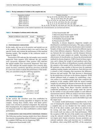
2) Logistic regression (LOG), RF, SVM, KNN, naive
Bayes classifier (NB) and feed forward neural network (FNN)
were used to establish CKD diagnostic models on the com-
plete CKD data sets. The models with better performance
were extracted for misjudgment analysis.
3) An integrated model that combines LOG and RF by
using perceptron was established and it improved the perfor-
mance of the component models in CKD diagnosis after the
missing values were filled by KNN imputation.
KNN imputation is used to fill in the missing values. To our
knowledge, this is the first time that KNN imputation has
been used for the diagnosis of CKD. In addition, building an
integrated model is also a good way to improve the perfor-
mance of separate individual models. The proposed method-
ology might effectively deal with the scene where patients
are missing certain measurements before being diagnosed.
In addition, the resulting integrated model shows a higher
accuracy. Therefore, it is speculated that this methodology
might be applicable to the clinical data in the actual medical
diagnosis.
The rest of the paper is organized as follows. In Section II,
we describe the preliminaries. The establishments of the
individual model and the integrated model are described in
Section III. In Section IV, we evaluate and discuss the perfor-
mance of the integrated model. In Section V, we summarize
the work and its contributions, including future works.
II. PRELIMINARIES
In this section, we describe the preliminaries before estab-
lishing the models, including the description of the data set
and the operating environment, the imputation of the missing
values and the extraction of the feature vector.
A. DATA DESCRIPTION AND OPERATING ENVIRONMENT
The CKD data set used in this study was obtained from the
UCI machine learning repository [32], which was collected
from hospital and donated by Soundarapandian et al. on 3rd
July, 2015. The data set contains 400 samples. In this CKD
data set, each sample has 24 predictive variables or features
(11 numerical variables and 13 categorical (nominal) vari-
ables) and a categorical response variable (class). Each class
has two values, namely, ckd (sample with CKD) and notckd
(sample without CKD). In the 400 samples, 250 samples
belong to the category of ckd, whereas 150 samples belong to
the category of notckd. It is worth mentioning that there is a
large number of missing values in the data. The details of each
variable are listed in Table 1. All of the algorithms were con-
ducted in R (version 3.5.2), and the packages used included
20992 VOLUME 8, 2020

3. J. Qin et al.: Machine Learning Methodology for Diagnosing CKD
TABLE 1. Details of each variable in the original CKD data set.
Hmisc(4.2-0), DMwR(0.4.1), leaps(3.0), randomForest
(4.6-14), caret(6.0-81), e1071(1.7-0.1), class(7.3-14) and
neuralnet(1.44.2).
B. DATA PROCESSING
Each categorical (nominal) variable was coded to facilitate
the processing in a computer. For the values of rbc and pc,
normal and abnormal were coded as 1 and 0, respectively. For
the values of pcc and ba, present and notpresent were coded
as 1 and 0, respectively. For the values of htn, dm, cad, pe and
ane, yes and no were coded as 1 and 0, respectively. For the
value of appet, good and poor were coded as 1 and 0, respec-
tively. Although the original data description defines three
variables sg, al and su as categorical types, the values of these
three variables are still numeric based, thus these variables
were treated as numeric variables. All the categorical vari-
ables were transformed into factors. Each sample was given
an independent number that ranged from 1 to 400. There is
a large number of missing values in the data set, and the
number of complete instances is 158. In general, the patients
might miss some measurements for various reasons before
making a diagnosis. Thus, missing values will appear in the
data when the diagnostic categories of samples are unknown,
and a corresponding imputation method is needed.
After encoding the categorical variables, the missing val-
ues in the original CKD data set were processed and filled at
first. KNN imputation was used in this study, and it selects the
K complete samples with the shortest Euclidean distance for
each sample with missing values. For the numerical variables,
the missing values are filled using the median of the corre-
sponding variable in K complete samples, and for the cate-
gory variables, the missing values are filled using the category
that has the highest frequency in the corresponding variable
in K complete samples. For physiological measurements,
people with similar physical conditions should have similar
physiological measurements, which is the reason for using
the method based on a KNN to fill in the missing values. For
example, the physiological measurements should be stable
within a certain range for healthy individuals. For diseased
individuals, the physiological measurements of the person
with a similar degree of the same disease should be similar.
In particular, the differences in physiological measurements
data should not be large for people with similar situations.
This method should also be adapted to the diagnostic data
of other diseases, as it has been applied in the area of
hyperuricemia [33].
When the median of corresponding variables in K com-
plete samples are selected, K is preferably taken as an odd
number because in this case the middle number is naturally
the median when the values of the numeric variables in the K
complete samples are sorted by numerical value. The selec-
tion of K should neither be too large nor too small. An exces-
sively large K value may ignore the inconspicuous mode,
which might be important. Conversely, an excessively small
K value causes noise and the abnormal data affects the filling
of the missing values exceedingly. Therefore, the values of K
in this work were chosen as 3, 5, 7, 9 and 11. As a result, five
complete CKD data sets were generated. In addition, we also
proved the effectiveness of KNN imputation by comparing it
with two other methods in section III. One is to use random
values to fill in the missing values, the other is to use mean
and mode of the corresponding variables to fill in missing
values of continuous and categorical variables, respectively.
C. EXTRACTING FEATURE VECTORS OR PREDICTORS
Extracting feature vectors or predictors could remove vari-
ables that are neither useful for prediction nor related to
response variables and thus prevent these unrelated variables
VOLUME 8, 2020 20993

4. J. Qin et al.: Machine Learning Methodology for Diagnosing CKD
FIGURE 1. The results of important variables extraction by using optimal subset regression at K = 9.
FIGURE 2. The results of important variables extraction by RF at K = 9.
from interfering with the model construction, which causes
the models to make an accurate prediction [34]. Herein,
we used optimal subset regression and RF to extract the
variables that are most meaningful to the prediction. Opti-
mal subset regression detects the model performance of all
possible combinations of predictors and selects the best com-
bination of variables. RF detects the contribution of each
variable to the reduction in the Gini index. The larger the Gini
index, the higher the uncertainty in classifying the samples.
Therefore, the variables with contribution of 0 are treated as
redundant variables. The step of feature extraction was run on
each complete data set. Images obtained on one complete data
set are shown in Figs. 1 and 2, and this data set was obtained
by KNN imputation when K equaling to 9.
Fig. 1 represents the optimal combination of variables in
the case of selecting one to all variables when the optimal
subset regression was used. The vertical axis represents vari-
ables. The horizontal axis is the adjusted r-squared which
represents the degree to which the combination of variables
explains the response variable. To make it easy to distin-
guish each combination of variables, we used four colors
(red, green, blue and black) to mark the selected variables.
The combinations are ranked from left to right by the degree
of explanations to the response variable and the right-most
combination has the strongest interception to the response
variable. Since the space is limited, the values represented by
the horizontal axis in Fig. 1 are retained in two decimal places.
The right-most combinations of variables in the images which
were obtained by the optimal subset regression on each com-
plete data set are shown in Table 2. For the complete data sets
obtained by the KNN imputation, we selected the intersection
of the optimal combinations on all complete data sets as
the extracted combination of variables to obtain a uniform
combination. In Table 2, for the complete data sets obtained
by the KNN imputation, we used the intersection (bp, sg, al,
bu, hemo, htn, dm, appet) to establish the models. For the
complete data set obtained by the mean and mode imputation,
the combination of the last row in Table 2 was used. For the
complete data sets obtained by random imputation, we used
the corresponding optimal combination obtained from each
complete data set.
The result of feature extraction of RF is represented
in Fig. 2, the vertical axis represents the variables, and the
horizontal axis represents the reduced Gini index. The larger
the reduced Gini index, the stronger the predictability of the
variable to the response variable. When the RF was used to
remove the variables with the contribution of zero, no matter
which method was used to fill in the missing values, the vari-
ables with contribution of zero were the same, including pcc,
ba and cad. Therefore, when the RF was used to extract the
variables, all variables were selected expect pcc, ba and cad.
20994 VOLUME 8, 2020

5. J. Qin et al.: Machine Learning Methodology for Diagnosing CKD
TABLE 2. The top combinations of variables on the complete data sets.
TABLE 3. The template of confusion matrix in this study.
D. PERFORMANCE INDICATORS
In this study, ckd was set to be positive and notckd was set
to be negative. The confusion matrix was used to show the
specific results and evaluate the performance of the machine
learning models. The template of the confusion matrix is
shown in Table 3.
True positive (TP) indicates the ckd samples were correctly
diagnosed. False negative (FN) indicates the ckd samples
were incorrectly diagnosed. False positive (FP) indicates
the notckd samples were incorrectly diagnosed. True nega-
tive (TN) indicates the notckd samples were correctly diag-
nosed. Accuracy, sensitivity, specificity, precision, recall and
F1 score were used to evaluate the performance of the model.
They are calculated using the following equations:
accuracy =
TP + TN
TP + FN + FP + TN
(1)
recall = sensitivity =
TP
TP + FN
(2)
specificity =
TN
FP + TN
(3)
precision =
TP
TP + FP
(4)
F1 score = 2 ×
precision × recall
precision + recall
(5)
III. PROPOSED MODEL
In this section, the classifiers were first established by
different machine learning algorithms to diagnose the data
samples. Among these models, those with better perfor-
mance were selected as potential components. By analyzing
their misjudgments, the component models were determined.
An integrated model was then established to achieve higher
performance.
A. ESTABLISHING AND EVALUATING INDIVIDUAL MODELS
The following machine learning models have been obtained
by using the corresponding subset of features or predictors on
the complete CKD data sets for diagnosing CKD.
1) Regression-based model: LOG
2) Tree-based model: RF
3) Decision plane-based model: SVM
4) Distance-based model: KNN
5) Probability-based model: NB
6) Neural network: FNN
Generally, in disease diagnosis, diagnostic samples are
distributed in a multidimensional space. This space comprises
predictors that are used for data classification (ckd or notckd).
Samples of data in the space are clustered in different regions
due to their different categories. Therefore, there is a bound-
ary between the two categories, and the distances between
samples in the same category are smaller. According to the
effectiveness of classification, we choose the aforementioned
methods for disease diagnosis. LOG is based on linear regres-
sion, and it obtains the weight of each predictor and a bias.
If the sum of the effects of all predictors exceeds a threshold,
the category of the sample will be classified as ckd or notckd.
RF generates a large number of decision trees by randomly
sampling training samples and predictors. Each decision tree
is trained to find a boundary that maximises the difference
between ckd and notckd. The final decision is determined
by the predictions of all trees in the disease diagnosis. SVM
divides different kinds of samples by establishing a deci-
sion surface in a multidimensional space that comprises the
predictors of the samples. KNN finds the nearest training
samples by calculating the distances between the test sample
and the training samples and then determines the diagnostic
category by voting. Naive Bayes classifier calculates the
conditional probabilities of the sample under the interval
by the number of ckd and notckd samples in each different
measurement interval. FNN can analyse non-linear relation-
ships in the data sets due to its complex structure, and the
sigmoid activation function was used in the hidden layer and
the output layer.
To evaluate model performance comprehensively, in the
case of retaining the sample distribution in the original data,
a complete data set was divided into four subsets evenly.
For all of the above models, each subset was utilized once
for testing, and other subsets were utilized for training,
the overall result was taken as the final performance. With
the exception of RF, the rest of the models were established
using the selected variables by feature extraction. RF does
not require prior feature extraction, because predictors are
selected randomly when each decision tree is established.
In addition, when using KNN and FNN, all the categorical
VOLUME 8, 2020 20995

6. J. Qin et al.: Machine Learning Methodology for Diagnosing CKD
TABLE 4. The accuracy of two types of RF after the KNN imputation was
run.
variables were converted into numeric types: categories 0 and
1 were converted to values 0 and 1, respectively, and the
complete data sets were then normalised with the mean that is
equal to 0 and the standard deviation that is equal to 1. Details
of all are as follows:
1) The output of LOG was the probability that the sample
belongs to notckd, and the threshold was set to 0.5.
2) RF was established using all variables. Two strategies
were used to determine the number of decision trees gen-
erated. One is to use the default 500 trees and the other is
to use the number of trees corresponding to the minimum
error in the training stage. The RF was established using both
strategies and evaluated on the data sets obtained by KNN
imputation. The same random number seed 1234 was used to
divide data and establish model, and the accuracy is shown
in Table 4. It can be seen that the default number of trees is
a better choice, therefore we selected the default 500 trees to
establish RF.
3) The models of SVM were generated by using the RBF
kernel function, and the function is described as follow:
Khx1, x2i = e−γ kx1−x2k2
(6)
where γ was set to [0.1, 0.5, 1, 2, 3, 4]. Parameter C
represents the weight of misjudgment loss, and it was set
to [0.5, 1, 2, 3]. In each calculation of the model training,
the algorithm selects the best combination of parameters to
establish the model by grid search.
4) For the NB, the value of Laplace was equal to 1.
5) For the KNN, due to the nearest Euclidean distance
with the detected sample, when the number of samples that
are selected in training data set is an even number, the algo-
rithm randomly selects a category as the output result of
the detected sample in the situation wherein the number of
selected samples belonging to ckd and notckd are the same.
To avoid this in the work, the nearest neighbor parameter was
set to [1, 3, 5, . . . , 19]. In each calculation of model training,
the algorithm selected the best parameter to establish the
model by grid search.
6) For the FNN, the network had a hidden layer. Presently,
there is no clear theory in determining the best number of
hidden layer nodes in a neural network. A method proposed in
the previous study that was used to evaluate the performance
of neural networks by increasing the number of hidden layer
nodes one by one [35] was used in this study. The number of
hidden layer nodes was increased one by one from 1 to 30.
Then, the best result was selected.
To ensure the repeatability and comparability of the results,
in the division of data, the establishment of RF with FNN,
and the selection of the best parameters of SVM with KNN,
the same seed of 1234 was used. For the random imputation,
TABLE 5. The accuracy (%) of the basic models after the optimal subset
regression.
TABLE 6. The accuracy (%) of the basic models after the features
extraction of RF was run.
the step of feature extraction was run on the complete data set
obtained. Then, the models were established and evaluated
by using the extracted features. Because of the randomness
of the random imputation, the whole process was repeated
five times to get the average result. For the KNN imputation
and the mean and mode imputation, due to the certainty
of data, the evaluation of models was executed once. After
the feature extraction methods of optimal subset regression
and RF were run, the accuracy of the basic models on
the complete data sets are shown in Table 5 and Table 6,
respectively.
It can been seen from Tables 5 and 6 that the optimal subset
regression is more suitable for LOG and SVM when the
KNN imputation is used, and the feature extraction method
of RF is more suitable for FNN and KNN. When the KNN
imputation is used, the accuracy of LOG and SVM is sig-
nificantly improved (Table 5). In Table 6, the accuracy of
LOG and SVM is relatively low, which might be due to the
fact that there are too many redundant variables compared
to the optimal subset regression. The accuracy of FNN is
slightly improved and RF shows better performance when
the KNN imputation is used both in Tables 5 and 6. For the
NB and the KNN, the performance of the models when using
KNN imputation is not very ideal compared to using random
imputation or mean and mode imputation in Tables 5 and 6.
The above result also proves the validity of the KNN impu-
tation, since KNN imputation does improve the accuracy of
some models, such as LOG, RF and SVM (Table 5). From
Tables 5 and 6, LOG and SVM with the use of optimal
subset regression, KNN and FNN with the use of the feature
extraction of random forest and RF have better performance.
Therefore, they are selected as the potential component
models.
20996 VOLUME 8, 2020

7. J. Qin et al.: Machine Learning Methodology for Diagnosing CKD
TABLE 7. The numbers of misjudgments of the extracted models.
B. MISJUDGMENT ANALYSIS AND SELECTING
COMPONENT MODELS
After evaluating the above models, the potential component
models were extracted for misjudgment analysis to determine
which would be used as the components. The misjudgment
analysis here refers to find out and compare the samples
misjudged by different models, and then determine which
model is suitable to establish the final integrated model.
The misjudgment analysis was performed on the extracted
models. The prerequisite for generating an integrated model
is that the misjudged samples from each component model
are different. If each component model misjudges the same
samples, the generated integrated model would not make a
correct judgement for the samples either. When the data were
read, each sample was given a unique number ranging from
1 to 400. The numbers of misjudgments for the extracted
models on each complete data are shown in Table 7, and the
black part indicates that the samples were misjudged by other
models except FNN.
In Table 7, for the FNN, it can be seen that most of
the misjudgments are simultaneously misjudged by other
models. In addition, the performance of FNN is affected
by the number of nodes in the hidden layer. It is not easy
to establish a unified model for different data. Therefore,
the FNN was excluded firstly. For the best model (RF), when
K equaling to 7, only one misjudgment is simultaneously
misjudged by the LOG. In other cases, all the samples that
are misjudged by RF can be correctly judged by the rest of
the models. Hence, the combinations of the RF with the rest
of the models could be used to establish an integrated model.
Next, we investigate which specific model combination could
generate the best integrated model for diagnosing CKD.
TABLE 8. The time spent by RF, LOG, SVM and KNN on the complete data.
From Tables 5 and 6, it can be seen that there is no significant
difference between LOG, SVM and KNN. In the case where
the performance of the models is similar, the models are
evaluated by the complexity of the algorithm, the running
time and the computational resources consumed. LOG, RF,
SVM and KNN were run five times on each complete data,
and the average time taken are summarized in Table 8. It can
be seen that the SVM and KNN take more time than the
LOG and RF. In addition, SVM and KNN are also effected
by their respective model parameters, so the parameters need
to be adjusted before the models are established, which means
more manual intervention is needed. For the LOG, there was
no additional parameter that need to be adjusted. For the
RF, the default parameters of the model were used. Hence,
a combination of the LOG and the RF was selected to generate
the final integrated model.
C. ESTABLISHING THE INTEGRATED MODEL
LOG and RF were selected as underlying components to
generate the integrated model to improve the performance
of judging. The probabilities that each sample was judged as
notckd in LOG and RF were used as the outputs of underlying
components. These two probabilities of each sample were
obtained and could be expressed in a two-dimensional plane.
In the complete CKD data sets, the probability distributions
of the samples in a two-dimensional plane are similar. There-
fore, the probability distribution of samples when K equaling
to 11 is shown in Fig. 3.
It can be seen from Fig. 3 that the samples have different
aggregation regions in the two-dimensional plane due to the
different categories (ckd or notckd). In general, samples with
ckd are concentrated in the lower left part, while the notckd
samples are distributed in the top right part. Due to the
fact that the results in the two models are different, some
samples are located at the top left and lower right, and one
of the two models makes the misjudgments. Perceptron can
be used to separate samples of two categories by plotting a
decision line in the two-dimensional plane of the probability
distribution. Ciaburro and Venkateswaran defined perceptron
as the basic building block of a neural network, and it can
be understood as anything that requires multiple inputs and
produces an output [36]. The perceptron used in this study is
shown in Fig. 4.
In Fig. 4, prob1 and prob2 are the probabilities that a sam-
ple was judged as notckd by LOG and RF, respectively. w0,
w1 and w2 are the weights of input signals. w0 corresponds
to 1, w1 corresponds to prob1 and w2 corresponds to prob2,
respectively. y is calculated according to (7):
y = w0 + w1 × prob1 + w2 × prob2. (7)
VOLUME 8, 2020 20997

8. J. Qin et al.: Machine Learning Methodology for Diagnosing CKD
FIGURE 3. The probability distribution of the samples in the complete
CKD data set (at K = 11), the horizontal axis and the vertical axis
represent the probabilities that the samples were judged as notckd by
the LOG and the RF, respectively.
FIGURE 4. The structure of the perceptron used in this study.
The input signal corresponding to the weight w0 is 1, which
is a bias. The function of Signum is used to calculate output
by processing the value of y as follows: If y > 0, then the
output = 1, whereas if y < 0, then the output = −1. For
the output, 1 corresponds to notckd, whereas -1 corresponds
to ckd. A single perceptron is a linear classifier that can be
used to detect binary targets. The weights are the core of the
perceptron and adjusted in the training stage. y = 0 is the
decision line, and this line can be described as (8):
prob2 = −
w1
w2
prob1 −
w0
w2
. (8)
In the training stage, the models of LOG and RF were
established by the training data at first. Then, a new training
data set was generated though combining the probabilities
of output of the two component models on the training data
and the labels of the samples. This new training data set was
used to establish the perceptron. For the binary classification,
the samples have two types of labels, i.e. Y = ±1. The
output of perceptron is calculated according to (7), we use
g(X) to represent the matrix form of this calculation, where
W = [w1, w2], X = [prob1, prob2]T , and b = w0. When the
g(X) > 0, the output = 1, whereas the g(X) < 0, then the
output = −1. Therefore, for all samples correctly judged by
the model, the following equation is valid:
Y × g(X) = Y(WX + b) > 0. (9)
For all misjudgments, the value of (9) is less than zero, and
the large the absolute value, the more serious the model mis-
judges the samples. Hence, for a misjudged sample (Xi, Yi),
the loss of the perceptron can be expressed as (10):
L = −Yi(WXi + b). (10)
The perceptron is trained by the gradient descent method to
adjust the weight and bias. The partial derivative of the weight
and bias of the loss function are expressed as follows:
∂L
∂W
= −YiXT
i (11)
∂L
∂b
= −Yi (12)
Therefore, in the training stage, for each misjudgment,
the weight and bias are updated by (13) and (14):
W = W + ηYiXT
i (13)
b = b + ηYi (14)
where the η is the learning rate.
However, for the bias, when the updating method of (14)
was used, the obtained decision line could classify the sam-
ples, but the line was located at the edge of the solution
area, so it is not reliable. To solve this problem, a new bias
adjustment strategy proposed in chapter 4 of the previous
literature [36] was referred and used, which is expressed in
(15):
b = b + ηYiR2
(15)
where the R is the maximum of the L2 norm of the eigen-
vectors in all training samples. When the (15) was used,
the obtained decision line could correctly classify the sam-
ples, and the line was located in the middle of the solu-
tion area, so it is more reliable than (14). When the second
subset was utilized for testing (at K = 11), the above phe-
nomenon was obvious. Figs. 5(a) and (b) plot the decision
line constructed by the perceptron on the training data set
when the updating strategies of (14) and (15) were used,
respectively. It can be seen that the updating strategy of (15)
in Fig. 5(b) is more reliable than (14) in Fig. 5(a). Therefore,
(13) and (15) were used as the updating strategies of the
perception. The pseudo code of the model is described as
follows:
Training stage
Input: Training data
Output: Integrated model (LOG, RF and perception).
Procedure
1. Use training data to train the model of LOG.
2. Use training data and default parameters to train the
model of RF.
3. Input training data into LOG and RF to record the
probabilities that the samples are judged as notckd by them.
20998 VOLUME 8, 2020

9. J. Qin et al.: Machine Learning Methodology for Diagnosing CKD
FIGURE 5. The decision line (blue line) obtained by the perceptron in the training data set. The horizontal axis and the
vertical axis represent the probabilities that samples were judged as notckd by models.
4. Build a new training data set, the predictors are the
probabilities of being recorded, and the response variable
is the label of training data.
5. Initialize the perceptron, W is randomly generated and
b is set to 0.
6. Traverse the samples in the new training data set. If (9)
is not satisfied, update W and b using (13) and (15).
7. Repeat step 6 until all of the sample satisfies (9).
8. Return LOG, RF and perception.
Testing stage
Input: Test data
Output: Sample category
Procedure
1. Input the data into LOG and RF to record the probabili-
ties that the samples are judged as notckd by them.
2. Input the probabilities into the perceptron to obtain the
result.
IV. EXPERIMENTS AND EVALUATIONS
In order to verify whether the integrated model can improve
the performance of the component models, we first used the
same random number seed 1234 to establish and evaluate
the integrated model on each complete data, and the con-
fusion matrices returned are shown in Table 9. Comparing
Tables 9 and 5, it can be found that the integrated model
improves the performance of the component models and
achieves an accuracy of 100% when K equaling to 3 and 11.
When K equaling to 5, 7 and 9, the integrated model improves
the performance of LOG and has the same accuracy with the
RF.
Next, for a comprehensive evaluation, we removed the
random number seed 1234 which was used to divide the
data into four subsets and establish the RF. The integrated
model was then run 10 times on the complete data sets. The
average results of the integrated models and two component
models are shown in Table 10, and the integrated model has
the best performance in detecting the two categories because
TABLE 9. The confusion matrices returned by the integrated models.
it achieves the highest accuracy and F1 scores under almost
all conditions. The accuracy and F1 scores of integrated
model have different degrees of improvement compared to
component models, and the sensitivity of components has
also been improved by integrated model. We can find that
the integrated model does improve the performance of the
component models and could achieve an ideal effect. We also
compared the methodology in this study (LOG, RF and inte-
grated model) with the other models on the same data in
previous studies (called contrast models), and the comparison
result is shown in Table 11. It can be seen that although the
performance of the LOG established in this work is relatively
low compared to some models established in previous studies,
it is still better than half of the contrast models. For the RF,
the performance is superior to most of the models built in
previous works, however, it is consistent with some mod-
els [29], [30]. The proposed integrated model improves the
performance of separate individual models and is superior to
almost all the contrast models, with the highest accuracy and
F1 score can achieve 100% in Table 9.
Our results show the feasibility of the proposed
methodology. By the use of KNN imputation, LOG, RF,
SVM and FNN could achieve better performance than the
VOLUME 8, 2020 20999

10. J. Qin et al.: Machine Learning Methodology for Diagnosing CKD
TABLE 10. Performance comparison between the LOG, RF and the proposed integrated model.
TABLE 11. Performance comparison between the other models and the proposed model on the same data.
cases when the random imputation and mean and mode
imputation were used. KNN imputation could fill in the
missing values in the data set for the cases wherein the diag-
nostic categories are unknown, which is closer to the real-life
medical situation. Through the misjudgments analysis, LOG
and RF were selected as the component models. The LOG
achieved an accuracy of around 98.75%, which indicates
most samples in the data set are linearly separable. The
RF achieved better performance compared with the LOG
with the accuracy was around 99.75%. From Tables 7 and 8,
the misjudgments produced by LOG and RF are differ-
ent in almost all cases, and the corresponding calculation
speeds are relatively fast. Therefore, an integrated model
combining LOG and RF was established to improve the
performance of the component models. From the simulation
result, the method of integrating several different classifiers
is feasible and effective. We speculate that this methodol-
ogy could be extended to more complex situations. When
processing more complex data, various different algorithms
are first attempted to establish models. After misjudgment
analysis, the better algorithms that produce different mis-
judgments are extracted as component models. An integrated
model is then established to improve the performance of the
classifier. From Tables 10 and 11, it can be seen that the
proposed methodology improves the performance of the oth-
erwise independent models and achieves comparable or better
performance compared to the models proposed in previous
studies. In addition, the CKD data set is composed of mixed
variables (numeric and category), so the similarity evaluation
methods based on mixed data could be used to calculate
the similarity between samples, such as general similarity
coefficient [37]. In this study, we used euclidean distance
to evaluate the similarity between samples, and KNN could
obtain a good result based on euclidean distance with the
highest accuracy of 99.25%. Therefore, we did not use other
methods to evaluate the similarity between samples.
V. CONCLUSION
The proposed CKD diagnostic methodology is feasible in
terms of data imputation and samples diagnosis. After unsu-
pervised imputation of missing values in the data set by
using KNN imputation, the integrated model could achieve
a satisfactory accuracy. Hence, we speculate that applying
this methodology to the practical diagnosis of CKD would
achieve a desirable effect. In addition, this methodology
might be applicable to the clinical data of the other diseases
in actual medical diagnosis. However, in the process of estab-
lishing the model, due to the limitations of the conditions,
the available data samples are relatively small, including only
400 samples. Therefore, the generalization performance of
the model might be limited. In addition, due to there are
only two categories (ckd and notckd) of data samples in the
21000 VOLUME 8, 2020

11. J. Qin et al.: Machine Learning Methodology for Diagnosing CKD
data set, the model can not diagnose the severity of CKD.
In the future, a large number of more complex and repre-
sentative data will be collected to train the model to improve
the generalization performance while enabling it to detect the
severity of the disease. We believe that this model will be
more and more perfect by the increase of size and quality of
the data.
ACKNOWLEDGMENT
J. Qin would like to thank the UCI machine learning
repository and the donators for sharing this CKD data set.
REFERENCES
[1] Z. Chen, Z. Zhang, R. Zhu, Y. Xiang, and P. B. Harrington, ‘‘Diagnosis
of patients with chronic kidney disease by using two fuzzy classifiers,’’
Chemometrics Intell. Lab. Syst., vol. 153, pp. 140–145, Apr. 2016.
[2] A. Subasi, E. Alickovic, and J. Kevric, ‘‘Diagnosis of chronic kidney
disease by using random forest,’’ in Proc. Int. Conf. Med. Biol. Eng.,
Mar. 2017, pp. 589–594.
[3] L. Zhang, ‘‘Prevalence of chronic kidney disease in China: A cross-
sectional survey,’’ Lancet, vol. 379, pp. 815–822, Mar. 2012.
[4] A. Singh, G. Nadkarni, O. Gottesman, S. B. Ellis, E. P. Bottinger, and
J. V. Guttag, ‘‘Incorporating temporal EHR data in predictive models for
risk stratification of renal function deterioration,’’ J. Biomed. Informat.,
vol. 53, pp. 220–228, Feb. 2015.
[5] A. M. Cueto-Manzano, L. Cortés-Sanabria, H. R. Martínez-Ramírez,
E. Rojas-Campos, B. Gómez-Navarro, and M. Castillero-Manzano,
‘‘Prevalence of chronic kidney disease in an adult population,’’ Arch. Med.
Res., vol. 45, no. 6, pp. 507–513, Aug. 2014.
[6] H. Polat, H. D. Mehr, and A. Cetin, ‘‘Diagnosis of chronic kidney disease
based on support vector machine by feature selection methods,’’ J. Med.
Syst., vol. 41, no. 4, p. 55, Apr. 2017.
[7] C. Barbieri, F. Mari, A. Stopper, E. Gatti, P. Escandell-Montero,
J. M. Martínez-Martínez, and J. D. Martín-Guerrero, ‘‘A new machine
learning approach for predicting the response to anemia treatment in a large
cohort of end stage renal disease patients undergoing dialysis,’’ Comput.
Biol. Med., vol. 61, pp. 56–61, Jun. 2015.
[8] V. Papademetriou, E. S. Nylen, M. Doumas, J. Probstfield, J. F. Mann,
R. E. Gilbert, and H. C. Gerstein, ‘‘Chronic kidney disease, basal insulin
glargine, and health outcomes in people with dysglycemia: The ORIGIN
Study,’’ Amer. J. Med., vol. 130, no. 12, pp. 1465.e27–1465.e39, Dec. 2017.
[9] N. R. Hill, ‘‘Global prevalence of chronic kidney disease—A system-
atic review and meta-analysis,’’ PLoS ONE, vol. 11, no. 7, Jul. 2016,
Art. no. e0158765.
[10] M. M. Hossain, R. K. Detwiler, E. H. Chang, M. C. Caughey, M. W. Fisher,
T. C. Nichols, E. P. Merricks, R. A. Raymer, M. Whitford, D. A. Bellinger,
L. E. Wimsey, and C. M. Gallippi, ‘‘Mechanical anisotropy assessment in
kidney cortex using ARFI peak displacement: Preclinical validation and
pilot in vivo clinical results in kidney allografts,’’ IEEE Trans. Ultrason.,
Ferroelectr., Freq. Control, vol. 66, no. 3, pp. 551–562, Mar. 2019.
[11] M. Alloghani, D. Al-Jumeily, T. Baker, A. Hussain, J. Mustafina, and
A. J. Aljaaf, ‘‘Applications of machine learning techniques for software
engineering learning and early prediction of students’ performance,’’ in
Proc. Int. Conf. Soft Comput. Data Sci., Dec. 2018, pp. 246–258.
[12] D. Gupta, S. Khare, and A. Aggarwal, ‘‘A method to predict diagnostic
codes for chronic diseases using machine learning techniques,’’ in Proc.
Int. Conf. Comput., Commun. Autom. (ICCCA), Apr. 2016, pp. 281–287.
[13] L. Du, C. Xia, Z. Deng, G. Lu, S. Xia, and J. Ma, ‘‘A machine learning
based approach to identify protected health information in Chinese clinical
text,’’ Int. J. Med. Informat., vol. 116, pp. 24–32, Aug. 2018.
[14] R. Abbas, A. J. Hussain, D. Al-Jumeily, T. Baker, and A. Khattak, ‘‘Classi-
fication of foetal distress and hypoxia using machine learning approaches,’’
in Proc. Int. Conf. Intell. Comput., Jul. 2018, pp. 767–776.
[15] M. Mahyoub, M. Randles, T. Baker, and P. Yang, ‘‘Comparison analysis
of machine learning algorithms to rank alzheimer’s disease risk factors
by importance,’’ in Proc. 11th Int. Conf. Develop. eSyst. Eng. (DeSE),
Sep. 2018, pp. 1–11.
[16] E. Alickovic and A. Subasi, ‘‘Medical decision support system for diagno-
sis of heart arrhythmia using DWT and random forests classifier,’’ J. Med.
Syst., vol. 40, no. 4, Apr. 2016.
[17] Z. Masetic and A. Subasi, ‘‘Congestive heart failure detection using ran-
dom forest classifier,’’ Comput. Methods Programs Biomed., vol. 130,
pp. 54–64, Jul. 2016.
[18] Q. Zou, ‘‘Predicting diabetes mellitus with machine learning techniques,’’
Frontiers Genet., vol. 9, p. 515, Nov. 2018.
[19] Z. Gao, J. Li, J. Guo, Y. Chen, Z. Yi, and J. Zhong, ‘‘Diagnosis of
diabetic retinopathy using deep neural networks,’’ IEEE Access, vol. 7,
pp. 3360–3370, 2019.
[20] R. J. Kate, R. M. Perez, D. Mazumdar, K. S. Pasupathy, and V. Nilakantan,
‘‘Prediction and detection models for acute kidney injury in hospital-
ized older adults,’’ BMC Med. Inform. Decis. Making, vol. 16, p. 39,
Mar. 2016.
[21] N. Park, E. Kang, M. Park, H. Lee, H.-G. Kang, H.-J. Yoon, and U. Kang,
‘‘Predicting acute kidney injury in cancer patients using heterogeneous and
irregular data,’’ PLoS ONE, vol. 13, no. 7, Jul. 2018, Art. no. e0199839.
[22] M. Patricio, ‘‘Using Resistin, glucose, age and BMI to predict the presence
of breast cancer,’’ BMC Cancer, vol. 18, p. 29, Jan. 2018.
[23] X. Wang, Z. Wang, J. Weng, C. Wen, H. Chen, and X. Wang, ‘‘A new
effective machine learning framework for sepsis diagnosis,’’ IEEE Access,
vol. 6, pp. 48300–48310, 2018.
[24] Y. Chen, Y. Luo, W. Huang, D. Hu, R.-Q. Zheng, S.-Z. Cong, F.-K. Meng,
H. Yang, H.-J. Lin, Y. Sun, X.-Y. Wang, T. Wu, J. Ren, S.-F. Pei, Y. Zheng,
Y. He, Y. Hu, N. Yang, and H. Yan, ‘‘Machine-learning-based classification
of real-time tissue elastography for hepatic fibrosis in patients with chronic
hepatitis B,’’ Comput. Biol. Med., vol. 89, pp. 18–23, Oct. 2017.
[25] E. Hodneland, E. Keilegavlen, E. A. Hanson, E. Andersen, J. A. Mon-
ssen, J. Rorvik, S. Leh, H.-P. Marti, A. Lundervold, E. Svarstad, and
J. M. Nordbotten, ‘‘In Vivo detection of chronic kidney disease using tissue
deformation fields from dynamic MR imaging,’’ IEEE Trans. Biomed.
Eng., vol. 66, no. 6, pp. 1779–1790, Jun. 2019.
[26] G. R. Vasquez-Morales, S. M. Martinez-Monterrubio, P. Moreno-Ger, and
J. A. Recio-Garcia, ‘‘Explainable prediction of chronic renal disease in the
colombian population using neural networks and case-based reasoning,’’
IEEE Access, vol. 7, pp. 152900–152910, 2019.
[27] Z. Chen, X. Zhang, and Z. Zhang, ‘‘Clinical risk assessment of
patients with chronic kidney disease by using clinical data and multi-
variate models,’’ Int. Urol. Nephrol., vol. 48, no. 12, pp. 2069–2075,
Dec. 2016.
[28] A. J. Aljaaf, D. Al-Jumeily, H. M. Haglan, M. Alloghani, T. Baker,
A. J. Hussain, and J. Mustafina, ‘‘Early prediction of chronic kidney
disease using machine learning supported by predictive analytics,’’ in Proc.
IEEE Congr. Evol. Comput. (CEC), Jul. 2018, pp. 1–9.
[29] B. Boukenze, A. Haqiq, and H. Mousannif, ‘‘Predicting chronic kidney
failure disease using data mining techniques,’’ in Proc. Int. Symp. Ubiqui-
tous Netw., Nov. 2016, pp. 701–712.
[30] N. A. Almansour, H. F. Syed, N. R. Khayat, R. K. Altheeb, R. E.
Juri, J. Alhiyafi, S. Alrashed, and S. O. Olatunji, ‘‘Neural network
and support vector machine for the prediction of chronic kidney dis-
ease: A comparative study,’’ Comput. Biol. Med., vol. 109, pp. 101–111,
Jun. 2019.
[31] W. Gunarathne, K. Perera, and K. Kahandawaarachchi, ‘‘Performance
evaluation on machine learning classification techniques for disease clas-
sification and forecasting through data analytics for chronic kidney disease
(CKD),’’ in Proc. IEEE 17th Int. Conf. Bioinf. Bioeng. (BIBE), Oct. 2017,
pp. 291–296.
[32] D. Dua and C. Graff, ‘‘UCI machine learning repository,’’ Ph.D. disserta-
tion, School Inf. Comput. Sci., Univ. California, Oakland, CA, USA, 2017.
[Online]. Available: http://archive.ics.uci.edu/ml.
[33] D. Ichikawa, T. Saito, W. Ujita, and H. Oyama, ‘‘How can machine-
learning methods assist in virtual screening for hyperuricemia? A health-
care machine-learning approach,’’ J. Biomed. Informat., vol. 64, pp. 20–24,
Dec. 2016.
[34] L. N. Sanchez-Pinto, L. R. Venable, J. Fahrenbach, and M. M. Churpek,
‘‘Comparison of variable selection methods for clinical predictive model-
ing,’’ Int. J. Med. Informat., vol. 116, pp. 10–17, Aug. 2018.
[35] G. Feng, G.-B. Huang, Q. Lin, and R. Gay, ‘‘Error minimized extreme
learning machine with growth of hidden nodes and incremental learn-
ing,’’ IEEE Trans. Neural Netw., vol. 20, no. 8, pp. 1352–1357,
Aug. 2009.
[36] G. Ciaburro and B. Venkateswaran, Neural Networks With R. Beijing,
China: China Machine Press, 2018, pp. 93–106.
[37] M. Hummel, D. Edelmann, and A. Kopp-Schneider, ‘‘Clustering of sam-
ples and variables with mixed-type data,’’ PLoS ONE, vol. 12, no. 11,
Nov. 2017, Art. no. e0188274.
VOLUME 8, 2020 21001

12. J. Qin et al.: Machine Learning Methodology for Diagnosing CKD
JIONGMING QIN received the B.S. degree in
electronic information engineering from Shanxi
University, China, in 2018. He is currently pursu-
ing the master’s degree with the Graduate School
of Electronic Information Engineering, Southwest
University, involving in the research of machine
learning and deep learning.
LIN CHEN received the B.S. degree in electronic
and information engineering from the School of
Electronics and Information Engineering, South-
west University, Chongqing, in 2018. He is cur-
rently pursuing the master’s degree with Kyushu
University, Fukuoka, Japan, in the research field
of gas and odor sensors.
YUHUA LIU received the B.S. degree in electronic
information engineering from the Chongqing Uni-
versity of Posts and Telecommunications, in 2016.
He is currently pursuing the master’s degree
in electronic and communication engineering
with Southwest University. His research inter-
ests include artificial intelligence and machine
learning.
CHUANJUN LIU received the Ph.D. degree in
material engineering from the Nagaoka University
of Technology, Japan, in 2006. He has been as a
Research Fellow with the Nagaoka University of
Technology, since 2006, and Kyushu University,
since 2018, where he has also been an Assistant
Professor with the Graduate School of Information
Science and Electrical Engineering, since 2012,
and an Associate Professor with the Research and
Development Center for Taste and Odor Sensing
(TAOS), since 2016. He is currently a Principle Researcher with the Research
Laboratory of U.S.E. Company, Ltd., Japan. His research interests include
the development and application of organic electronic devices, nanoscale
sensing materials, and gas and odor sensors. He is a member of the Society of
Polymer Science Japan and the Institute of Electrical Engineering of Japan.
CHANGHAO FENG received the M.S. degree
from the Department of Electronic Sciences
and Technology, Heilongjiang University, China,
in 2012, and the Ph.D. degree from Jilin Univer-
sity, China, in 2016. He is currently a Lecturer
with the College of Electronic and Information
Engineering, Southwest University, and involving
in the research of gas sensors.
BIN CHEN received the Ph.D. degree from
the Graduate School of Information Science and
Electrical Engineering, Kyushu University, Japan,
in 2014. She is currently an Associate Professor
with the College of Electronic and Information
Engineering, Southwest University. She is a JSPS
Fellow work with Kyushu University, involving in
the research of chemical sensors, portable gadget
and device development, and machine learning.
21002 VOLUME 8, 2020