With Nathan Lindle. ANTS VIII, 2008.

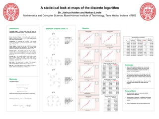
1. A statistical look at maps of the discrete logarithm
Dr. Joshua Holden and Nathan Lindle
Mathematics and Computer Science, Rose-Hulman Institute of Technology, Terre Haute, Indiana 47803
Definitions Example Graphs (mod 11) Results
Functional Graph – A directed graph where the edges are
determined by a transition function. In this case the function is
g=3
Binary Functional Graph – A functional graph where the in-
Components: 2 Sample Maximum Tail Statistics
degree of each node is either 0 or 2. All the graphs studied
Cyclic nodes: 4 Mean Std. Dev.
were binary functional graphs.
Average cycle: 2.2
p Predicted Observed P‐value Observed
Average tail: 0.8
Component - A connected set of nodes. The average 99923 547.605802 543.281073 0 163.809
Max cycle: 3
number of components is measured for each prime modulus
(e.g. 1.75 for p = 11)
Max tail: 2 99961 547.710225 541.005022 0 163.494
99971 547.737702 544.967041 0.002 165.249
Cyclic Nodes – Nodes that are part of a cycle, including 99989 547.787156 542.47563 0 163.809
nodes which loop back on themselves. The average cyclic
99991 547.792651 541.265167 0 163.805
nodes are measured for each prime (e.g. 3.25 for p = 11)
100003 547.825617 543.876996 0 163.295
Average Cycle – The average cycle size as seen from a 100019 547.86957 542.008421 0 163.79
random node in a functional graph divided by the number of 100049 547.951971 544.38604 0.002 165.651
nodes in all the functional graphs for a given prime (e.g. 2.05
for p = 11) 100069 548.006899 549.379291 0.318 165.926
g=4
100103 548.100263 540.966673 0 164.496
Average Tail – The average distance to the cycle as seen
from a random node in the graph. Cyclic nodes have a
distance of 0. Computation is similar to that of the average Components: 1
cycle (e.g. 1.225 for p = 11) Cyclic nodes: 2
Average cycle: 2
Max Cycle – The largest cycle in a graph. The average is Average tail: 2
taken over all bases for a given p (e.g. 2.5 for p = 11) Max cycle: 2 Sample Average Cycle Std. Dev.
Max tail: 4 p Predicted Observed
Max Tail – The longest distance from a node to its cycle in a 99923 164.857 143.637
Summary
graph. Similar to max cycle (e.g. 2.75 for p = 11) • Many of the statistics gathered do not provide
99961 164.888 140.91
99971 164.897 143.442 sufficient evidence to question the theory that
g=5 99989 164.911 144.856 modular exponentiation graphs are similar to
99991 164.913 143.678 random functional graphs.
100003 164.923 143.686
100019 164.936 143.632 • The observed variance in the average cycle and
100049 164.961 142.121
the average tail were significantly lower than the
100069 164.978 143.612
Components: 2 expected variance for a random binary functional
100103 165.006 142.79
Cyclic nodes: 3 graph.
Methods Average cycle: 1.4 Sample Average Tail Std. Dev.
Average tail: 1.3 p Predicted Observed • A few tests had surprisingly low p-values, but the
Generating functions:
Max cycle: 2 99923 164.858 86.025 normality tests indicate that these were just
Max tail: 3 99961 164.89 85.319 outliers.
99971 164.898 86.914
99989 164.913 85.661
99991 164.914 85.227
100003 164.924 85.261
100019 164.938 86.029
100049 164.962 86.398 Future Work
g=9 100069 164.979 87.876
Marked generating function for total number of components: 100103 165.007 86.234
• Get theoretical values for maximum tail and
maximum cycle variance.
Sample Max Cycle Std. Dev.
Components: 2
p Observed • Analyze lower variances in average cycle length
Generating function for total number of components: Cyclic nodes: 4 99923 154.949 and average tail length to try and come up with a
Average cycle: 2.6 99961 152.417 reason.
Average tail: 0.8 99971 154.931
Max cycle: 3 99989 156.06
Max tail: 2 • Find an explanation for the lower maximum tail.
99991 154.534
100003 154.874
100019 154.535
100049 153.792
100069 155.018
100103 154.1