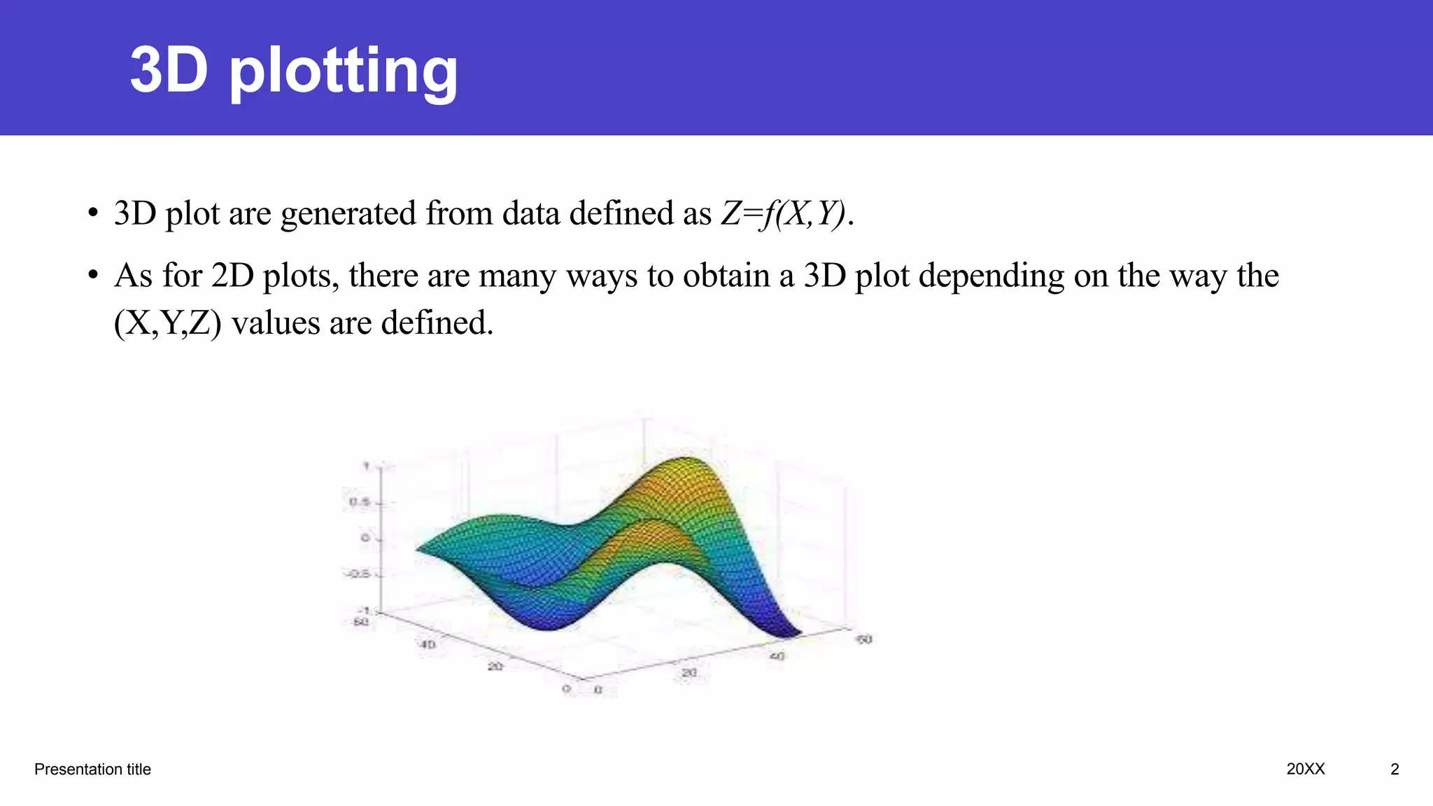
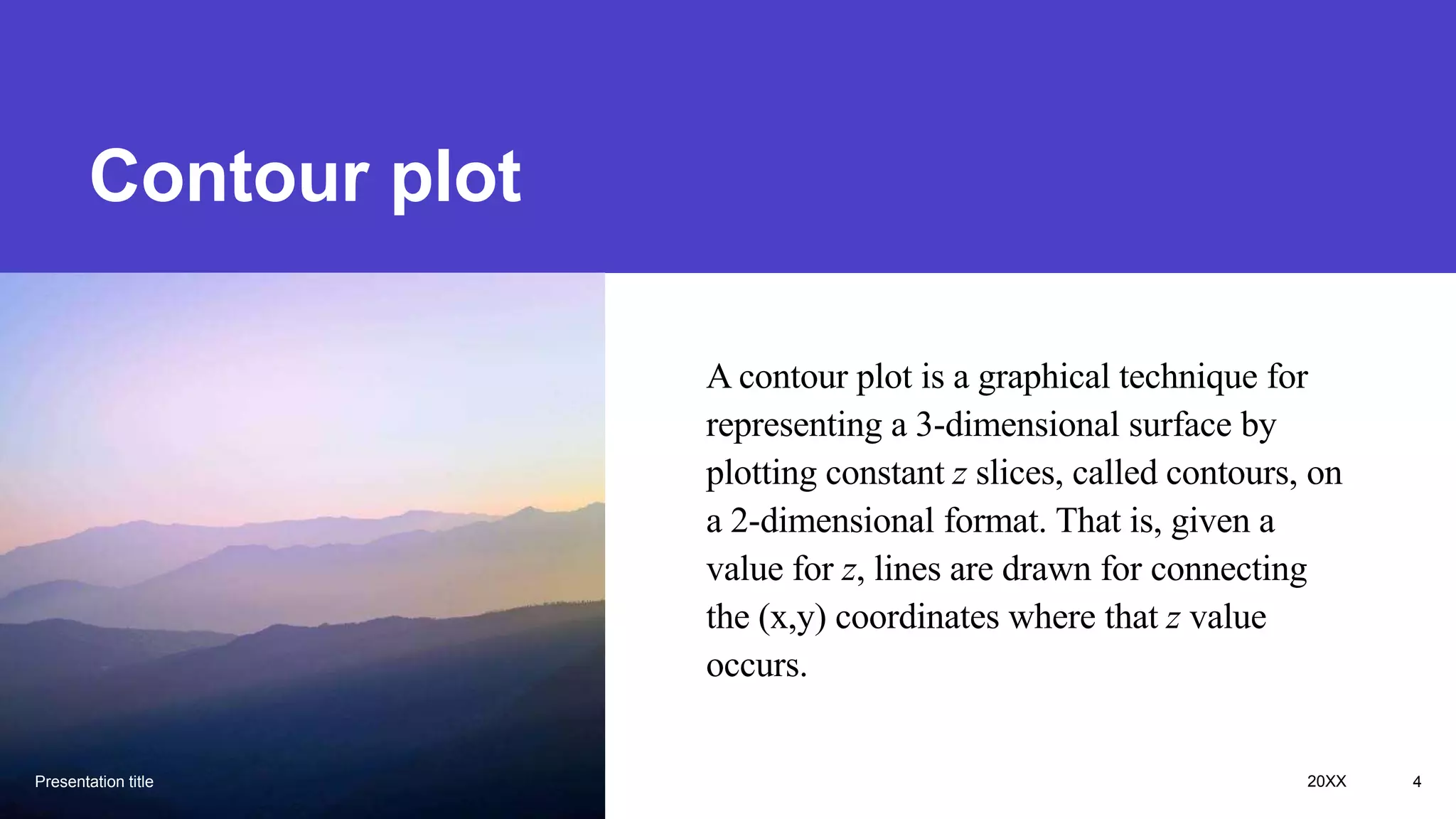
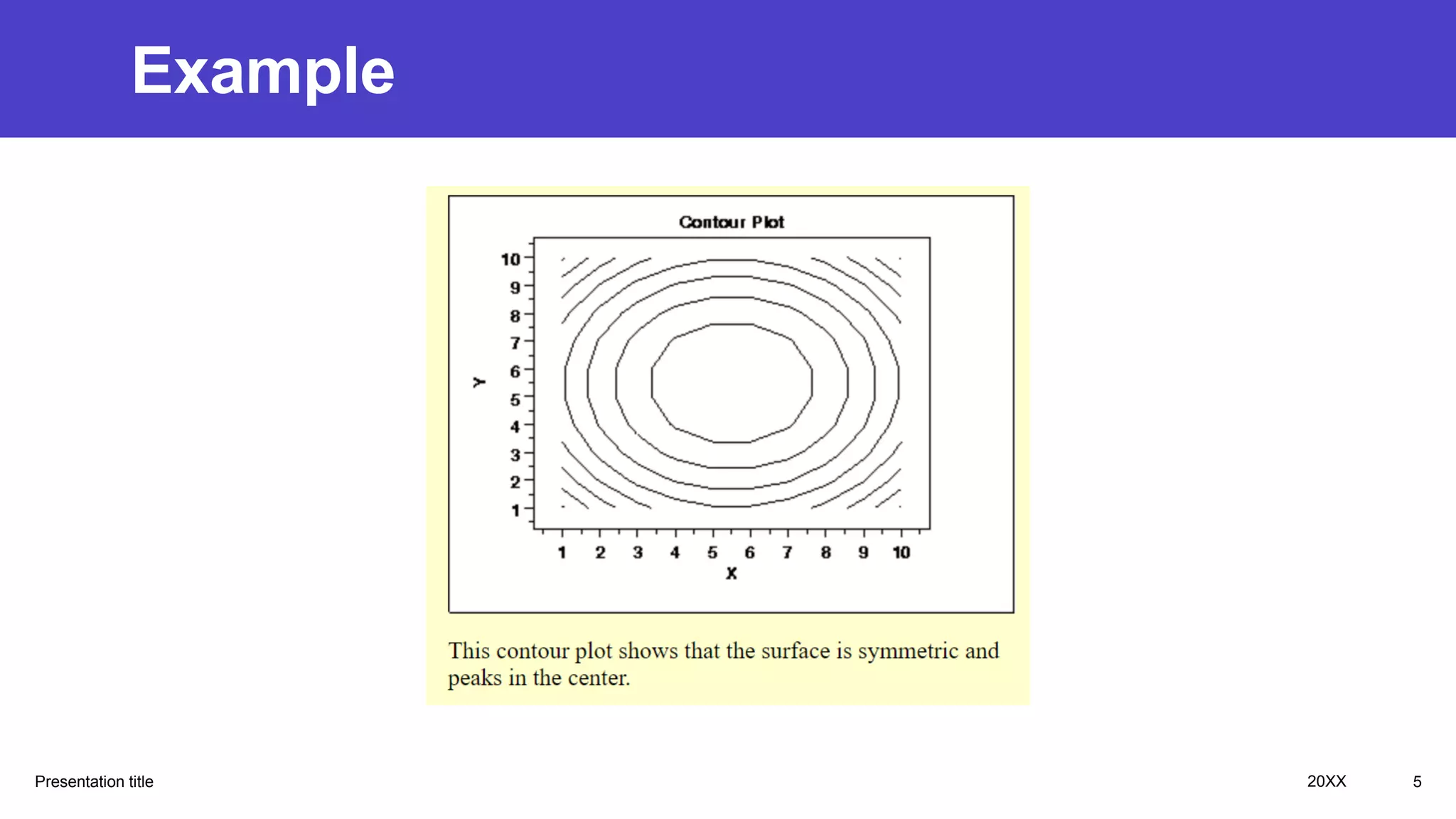
3D plots are generated from data defined as Z=f(X,Y), with Plot3D[] being the main code. Contour plots represent a 3D surface by plotting constant z slices called contours on 2D, drawing lines connecting (x,y) coordinates with the same z value. ContourPlot[] is the main code, and examples can be found in Mathematica files.

1. 3D plotting
and contour
plotting
Areej Fatima

2. 3D plotting
• 3D plot are generated from data defined as Z=f(X,Y).
• As for 2D plots, there are many ways to obtain a 3D plot depending on the way the
(X,Y,Z) values are defined.
Presentation title 20XX 2

3. Code
Presentation title
• Plot3D [] .. This is the main code for 3D plotting
• Plot3D [equation/function , {variable,
min,max},{var,min,max}]
• Consult Mathematica files for examples.
20XX 3

4. Contour plot
Presentation title
A contour plot is a graphical technique for
representing a 3-dimensional surface by
plotting constant z slices, called contours, on
a 2-dimensional format. That is, given a
value for z, lines are drawn for connecting
the (x,y) coordinates where that z value
occurs.
20XX 4

5. Example
Presentation title 20XX 5

6. Code
Presentation title
• ContourPlot [] .. This is the main code for 3D plotting
• ContourPlot[equation/function , {variable,
min,max},{var,min,max}]
• Consult Mathematica files for examples.
20XX 6

7. The way to get
started is to quit talking
and begin doing.
Walt Disney
Presentation title 20XX 7

8. Thank you
Areej Fatima
Presentation title 20XX 8