3a The Dynamic Implications of Sequence Risk on a Distribution Portfolio JFP Jun 2010.pdf

52 Journal of Financial Planning | JU N E 2010 www.FPAjournal.org
Contributions
Larry R. Frank Sr., CFP®, a wealth adviser and author,
lives in Rocklin, California. He has combined an MBA
with a finance concentration from the University of South
Dakota with a BS cum laude physics from the University
of Minnesota to bring the time dimension into the dynam-
ics of retirement distributions in personal finance.
David M. Blanchett, CFP®, CLU, AIFA®, QPA, CFA, is an
institutional consultant at Unified Trust Company in
Lexington, Kentucky. He oversees fiduciary, compliance,
operational, and investment issues relating to Unified
Trust’s retirement plan and wealth management services.
He won the Journal of Financial Planning’s 2007
Financial Frontiers Award with a paper titled
“Determining the Optimal Distribution Glide Path.”
S
equence risk, or the effect of
returns on the probability of suc-
cess for a distribution portfolio, is
a timely issue. The stock market decline in
2008 left many retirees, and their advisers,
questioning the long-term sustainability of
their distribution portfolio. When markets
drop and force a higher than sustainable
withdrawal rate, advisers and their clients
are left with many questions: How does
one recognize and manage such inadver-
tent exposure? Is this exposure the same
with different portfolio allocations? Is this
exposure the same as the retiree ages?
Does sequence risk ever really go away?
Unlike past research, which has sug-
gested sequence risk only exists for a cer-
tain period, the authors contend that a
“spectrum” of exposure to sequence risk
exists, and that sequence risk is always
present, regardless of how long distribu-
tions have been occurring. This paper will
discuss this exposure to sequence risk and
argue that sequence risk is always present
to some degree when there are cash flows
The Dynamic Implications of Sequence
Risk on a Distribution Portfolio
by Larry R. Frank Sr., CFP®
, and David M. Blanchett, CFP®
, CLU, AIFA®
, QPA, CFA
FR A N K | BL A N C H E T T
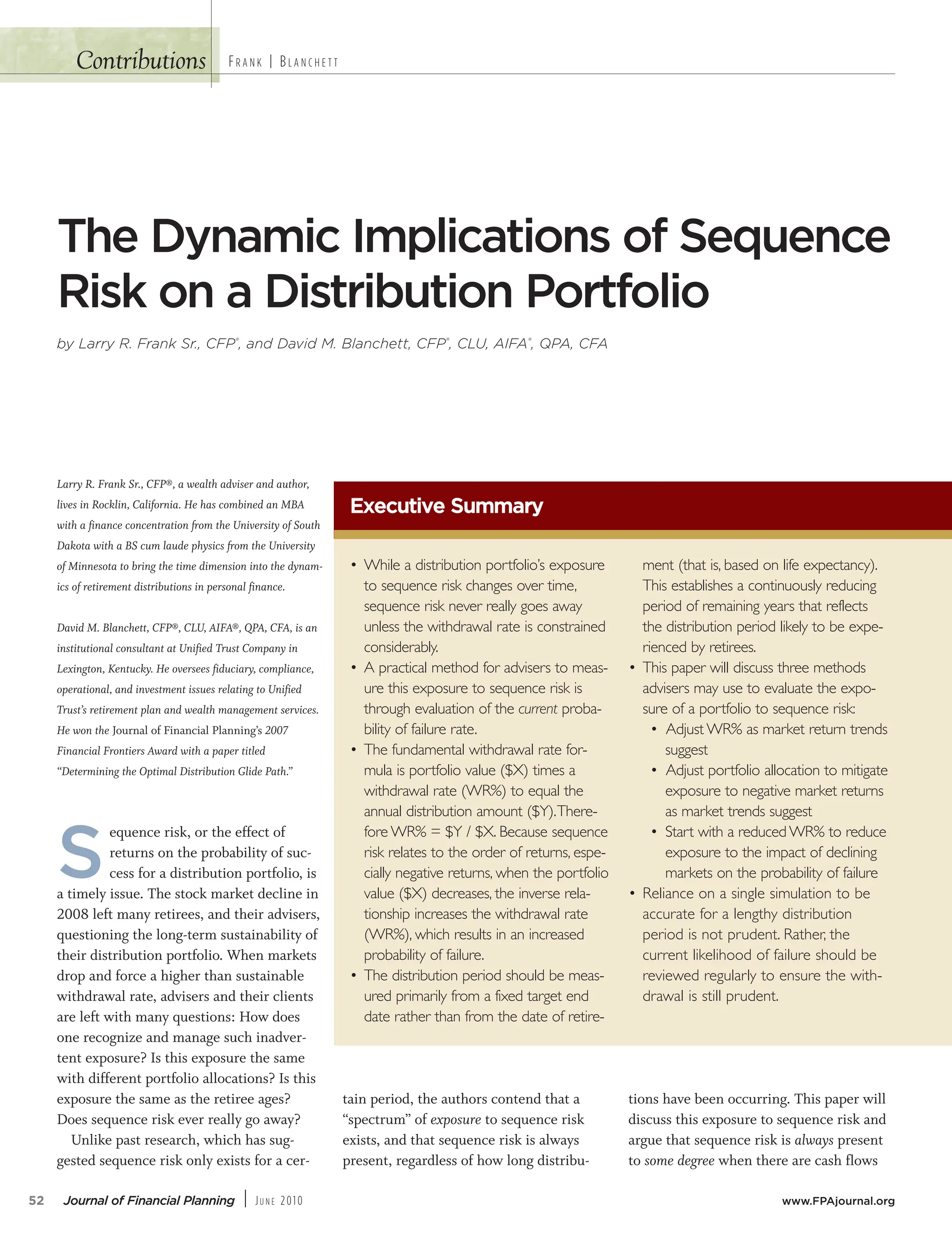
• While a distribution portfolio’s exposure
to sequence risk changes over time,
sequence risk never really goes away
unless the withdrawal rate is constrained
considerably.
• A practical method for advisers to meas-
ure this exposure to sequence risk is
through evaluation of the current proba-
bility of failure rate.
• The fundamental withdrawal rate for-
mula is portfolio value ($X) times a
withdrawal rate (WR%) to equal the
annual distribution amount ($Y).There-
fore WR% = $Y / $X. Because sequence
risk relates to the order of returns, espe-
cially negative returns, when the portfolio
value ($X) decreases, the inverse rela-
tionship increases the withdrawal rate
(WR%), which results in an increased
probability of failure.
• The distribution period should be meas-
ured primarily from a fixed target end
date rather than from the date of retire-
ment (that is, based on life expectancy).
This establishes a continuously reducing
period of remaining years that reflects
the distribution period likely to be expe-
rienced by retirees.
• This paper will discuss three methods
advisers may use to evaluate the expo-
sure of a portfolio to sequence risk:
• Adjust WR% as market return trends
suggest
• Adjust portfolio allocation to mitigate
exposure to negative market returns
as market trends suggest
• Start with a reduced WR% to reduce
exposure to the impact of declining
markets on the probability of failure
• Reliance on a single simulation to be
accurate for a lengthy distribution
period is not prudent. Rather, the
current likelihood of failure should be
reviewed regularly to ensure the with-
drawal is still prudent.
Executive Summary

Contributions
out of the portfolio. This paper will also
demonstrate that the degree of exposure
can be determined through evaluation of
the current probability of failure of the
portfolio’s value being depleted during the
remaining distribution period.
As a practical matter, sequence risk
depends on the degree of cash flow relative
to the direction of the portfolio value’s
trend. Sequence risk is only really a con-
cern when the value of a portfolio drops
combined with an ongoing cash flow
requirement (for example, lifetime income
for a retiree). An increase in the value of a
portfolio does not increase sequence risk
and, while it is possible for a portfolio with
no cash-flows to experience sequence risk
(for example, just before retirement), out-
going cash flows are typically required.
The fundamental withdrawal rate for-
mula is portfolio value ($X) times a with-
drawal rate (WR%) to equal the annual dis-
tribution amount ($Y). Therefore WR% =
$Y / $X. Because sequence risk relates to
the order of returns, especially negative
returns, as the denominator value $X (or
portfolio account balance) decreases, the
inverse relationship forces WR% higher,
which translates to a higher probability of
failure, a direct relationship with WR%.
Literature Review
Recent market events have increased the
available literature on sequence risk, a
topic that had not received much scrutiny
in the past. Furthermore, Mitchell (2009)
states, “Existing research does not address
the question of acceptable probabilities of
failure (running out of money before the
end of the planning horizon) …” where
acceptable is an explicitly defined limit or
zone, rather than a value determined and
then unmonitored once distributions have
begun. Milevsky (2006) writes, “The first
decade of retirement is the most crucial
one in determining whether your retire-
ment plan will be successful.” Continuing,
“It seems that the first seven years of
retirement are the most crucial in affecting
the probability of ruin.” The implication is
that, as time passes, the risk of ruin sub-
sides. This observation emanates from
referring to the date the withdrawals began
and then counting forward from that date.
This creates a time paradox. For example,
how can it be that the sequence risk for a
couple that is 10 years into their projected
40-year retirement period be different than
that for a couple about to retire with a pro-
jected 30-year distribution period? The real
question that a retiree should be asking is,
“What is the current probability of ruin for
the current exposure to a detrimental
market?” Because time is dynamic, and
withdrawals are taken currently, the start-
ing point for measur-
ing sequence risk
should always be
from the present
going forward.
Time Measurement
With traditional
retirement distribu-
tion thinking, both
measurement points,
retirement age and
average mortality age, actually “float with
time” as the retiree ages. The authors’
convention in this paper is to fix the mor-
tality age point, called “target end date,”
so that measurement of distribution peri-
ods dynamically reflect time remaining
from the current retirement age as the
retiree ages. Previous research has demon-
strated that age 95 is a reasonable target
end date for a retiring couple (Blanchett
2008) as well as individuals (Frank 2009).
Trying to “fudge” a shorter target end date
through rationalization of disease or sick-
ness may be fraught with risk through
unforeseen medical advances and cures.
However, selecting a distribution period
that is too long subjects the retirees to
under consumption, meaning they could
have consumed more during their life-
times. Therefore, when determining the
length of the distribution period, the esti-
mate should be neither too conservative
nor too aggressive.
What Is Sequence Risk?
When considering sequence risk, it is first
important to separate the order of returns
from the returns themselves. Monte Carlo
simulations involve generating a random
series of returns dispersed around a mean
return, with the variability defined by the
standard deviation. To demonstrate why
and how return order (or more generally,
sequence risk) is important, an iterative
simulation of 10,000 runs was conducted
based on various equity allocations (which
correspond to historical real rates of return
and historical standard deviations) for a
30-year distribution period based on a 5
percent initial real withdrawal rate.
For this simulation, though, the returns
for each of the runs are “equalized” so that
the simulation has the same real rate of
return for the entire 30-year distribution
period. Therefore, the only difference in
the individual simulations would be order
(sequence) or returns experienced by the
portfolio. This method was used so as to
“isolate” and control other return factors to
demonstrate the effect of sequence risk on
a portfolio, and the results are included in
Figure 1.
Figure 1 demonstrates that even when
the return for the entire period in each test
run is the same, there can still be a consid-
erable dispersion in the potential probabil-
ity of failure. The key is when the low
returns are realized. Those runs that fail
tend to have lower than average initial
returns (and above average ending
returns), while the runs that pass have
www.FPAjournal.org JU N E 2010 | Journal of Financial Planning 53
“Even when you equalize the total
period returns for a simulation, some runs
may fail while others pass, the reason being
the order, or sequence, in which they are
experienced.
”

Contributions
higher than average initial returns (and
below average ending returns). To summa-
rize, even when you equalize the total
period returns for a simulation, some runs
may fail while others pass, the reason
being the order, or sequence, in which they
are experienced. Brayman (2009) found
similar results; lucky or unlucky sequence
of events explained more of the phenome-
non than over- or under-achieving
expected returns. This concept is demon-
strated visually in Figure 2, where the aver-
age returns of passing runs and failing runs
are separated for a single simulation.
What Happens to Sequence Risk over Time?
While it is commonly assumed that
sequence risk “goes away,” sequence risk is
actually something that is always present.
With time, the portfolio tends to move into
a range of either certain failure or certain
success. This is why withdrawal rates
should be lower for longer distribution
periods and may be higher for shorter dis-
tribution periods, with an equal exposure to
probability of failure (Figure 3).
First generation withdrawal thinking has
been to establish an initial withdrawal rate
(WR%) and then adjust the resulting dollar
distribution ($Y) for inflation. Thus, the
withdrawal rate is not directly adjusted,
because an initial dollar amount is
increased (decreased) for inflation (defla-
tion). However, when the stock market
falls, the current withdrawal rate (the with-
drawal as a percentage of the portfolio
assets) increases, potentially dramatically,
due to the inverse relationship of the dollar
distribution to the portfolio value.
For example, if a portfolio were to drop
in value by 25 percent, a retiree with a $1
million portfolio and a $40,000 withdrawal
would see the withdrawal rate as a percent-
age of total assets increase from 4 percent
($40,000/$1 million) to 5.33 percent
($40,000/$750,000) (not including the
annual withdrawal). Clearly, a 5.33 percent
distribution rate has a higher probability of
failure than a 4 percent distribution rate
for the same distribution period. Such a
relative change in portfolio value can occur
at anytime during the retiree’s lifetime.
This concept is illustrated graphically in
Figure 3, which reflects the probability of
failure for various periods based on the ini-
tial real withdrawal rate and the real return
of the portfolio in the first year for a 60/40
portfolio (that is, the return for the first
year is listed on the y-axis, and the follow-
ing returns are randomized). The graphs
for the time periods in Figure 3 have been
arranged to demonstrate the fact that the
probability of failure “ticks down” to a ter-
mination date/age.
Moving from Uncertainty to Certainty
As a distribution portfolio moves through
time, the “uncertainty” of its outcome
declines. At the beginning of most Monte
Figure 2: Return Differences BetweenThose Portfolios that Passed and
Failed for the 30% Equity Portfolio
0.00%
1.00%
2.00%
3.00%
4.00%
5.00%
6.00%
1 4 7 10 13 16 19 22 25 28
Real
Average
Geometric
Rate
of
Return
Distribution Year
Runs that Failed Runs that Passed Portfolio Average
Figure 1:
0%
10%
20%
30%
40%
50%
60%
70%
80%
90%
100%
1.8% 2.5% 3.0% 3.6% 4.2% 4.7% 5.2% 5.7% 6.1% 6.6% 7.0%
Percentage
of
Total
Runs
Portfolio Rate of Return
Runs that Failed Runs that Passed
Probability of Failure forVarious Equity Allocations with 30-Year
Distribution Period and a 5% Initial RealWithdrawal Rate

Contributions
Carlo simulations, the probability of
achieving a goal is defined by a certain
probability. What happens, though, if you
“revisit” the probability of the portfolio
successfully achieving its goal through
time? Doing so allows the individual to see
that the uncertainty associated with the
outcome moves to one of two outcomes:
certain success or certain failure. This con-
cept is demonstrated in Figure 4, which
shows the range of “uncertain” outcomes
where the probability of failure is between
5 percent and 95 percent (a probability of
failure below 5 percent is deemed to be
certain success while a probability of fail-
ure above 95 percent is deemed to be cer-
tain failure). Figure 4 demonstrates the con-
cept of how in the absence of any type of
intervention (for example, changing the port-
folio allocation or the withdrawal rate) the
uncertainty surrounding the outcome of a
given decumulation decreases through time.
Referring to the time measurement dis-
cussion above, imagine all the end points in
Figure 4 set at the client’s calendar age 95.
This helps emphasize the current year range
of outcomes illustrated and the changing
nature of withdrawal rates with time.
Taking an Adaptive Approach to Distribution
Planning to Manage Exposure to Sequence Risk
Previous research by Blanchett and Frank
(2009) introduced a relatively simple frame-
work for adjusting the annual real with-
drawal from a distribution portfolio based on
the ongoing probability of success of the
portfolio. By recalculating the probability of
portfolio failure each year (that is, replicate
the methodology that financial planners typi-
cally employ when working with clients) it
becomes possible to make adjustments if
sequence risk becomes an issue. The authors
suggested that exposure to sequence risk is
recognizable when the probability of failure
(of the same portfolio allocation and same
withdrawal dollar amount) begins to rise.
The probability of failure begins to go up
when the current withdrawal rate goes up.
For the revisiting strategy, the probability
of failure was calculated for each year of each
run of each scenario to replicate the dynamic
approach an adviser may take when working
with a retired client as markets change. The
withdrawal stayed the same, increased, or
decreased based on the probability of success
for the current withdrawal rate. Figure 5
demonstrates the various success rates for a
distribution strategy without revisiting (that
is, when the withdrawal does not change)
and with revisiting (that is, when the with-
drawal changes are based on the projected
probability of success for the portfolio). Simi-
lar to Figure 4, the reader can see in Figure 5
that the uncertainty associated with a given
simulation decreases through time.
Figure 5 suggests it is possible to recognize
exposure to sequence risk and make adjust-
ments to a portfolio to improve the likeli-
hood of retirement success. Two actions
directly under the client’s control are: (1)
reduce the portfolio’s exposure to decline
through a change in the asset allocation or
(2) reduce the portfolio’s distributions (that
is, a retiree pay cut).
Figure 3: Comparison ofVariousWithdrawal Rates withVarying First
Year Portfolio Returns for Different Distribution Periods
(60/40 Portfolio)
Portfolio
Return
in
the
First
Distribution
Year
40-Year Distribution Period, 5% Real
Return & 10% Annual Standard Deviation
20%
15%
10%
5%
0%
-5%
-10%
-15%
-20%
-25%
-30%
-35%
-40%
Portfolio
Return
in
the
First
Distribution
Year
20%
15%
10%
5%
0%
-5%
-10%
-15%
-20%
-25%
-30%
-35%
-40%
Portfolio
Return
in
the
First
Distribution
Year
20%
15%
10%
5%
0%
-5%
-10%
-15%
-20%
-25%
-30%
-35%
-40%
Portfolio
Return
in
the
First
Distribution
Year
20%
15%
10%
5%
0%
-5%
-10%
-15%
-20%
-25%
-30%
-35%
-40%
Initial Real Withdrawal Rate
3% 4% 5% 6% 7% 8% 9% 10% 3% 4% 5% 6% 7% 8% 9% 10%
3% 4% 5% 6% 7% 8% 9% 10% 3% 4% 5% 6% 7% 8% 9% 10%
Corresponding Color Probability of Failure Relative Likelihood
0%–5%
6%–25%
26%–50%
51%–75%
76%–95%
96%–100%
Highly Unlikely
Unlikely
Not Probable
Probable
Likely
Highly Likely

Contributions
Probability of Failure Trajectories
The basic formula WR% = $Y / $X is a
generalized form where key defining sub-
scripts are not displayed. Each WR% has
associated with it a probability of failure
(POF) for a given remaining distribution
time (t), which is displayed in Figure 6.
This information is obtained from Figure 2
in Blanchett and Frank (2009). Note that
different portfolio allocations and with-
drawal strategies would have different
graphs published in the previous paper.
The simulations in Figure 6 are based on
a constant distribution period and assume
a static withdrawal rate. WR% may be writ-
ten more specifically for this discussion as
WR% (POF, t) to accentuate the relation-
ships between time, withdrawal rate, and
probability of failure.1 Introducing a
dynamic remaining distribution time (t)
variable helps explain why a withdrawal
rate WR%, for example 9 percent for t=10,
may be greater than a withdrawal rate of 4
percent for t=30, and yet both have similar
probability of failure rates (0 percent–5
percent) as they both lie on the same prob-
ability of failure trajectory (upper edge of
the green zone). As the portfolio value
increases or decreases as a function of
market value, WR% (POF, t) varies inversely
along the probability of failure trajectory.
In other words, when t is held constant, for
a decreasing portfolio value $X (denomina-
tor), the probability of failure goes up
because the withdrawal rate has increased
relative to a set annual withdrawal $Y, or
vice versa. However, t is not constant.
A different way to visualize Figure 6
would be to determine withdrawal rates for
various time periods and withdrawal rates
with the same approximate probability of
failure. This has been done in Figure 7,
where the probability of failure for each of
the simulations is 0 percent–5 percent
(that is, deemed highly unlikely). Higher
threshold landscapes (for example, Figure
6’s yellow zone) would map out higher on
the x-axis compared to the 0 percent–5
percent threshold illustrated, because cor-
responding withdrawal rates are higher. In
other words, the 0 percent–5 percent land-
scape is the lowest probability of failure
landscape. Note that as distribution time
shortens, withdrawal rates may increase,
all with a similar approximate exposure to
Advisers and their clients should deter-
mine, based on client circumstances, what
an appropriate probability of failure deci-
sion threshold should be. For example, a
retiree with little discretionary flexibility
should have a lower threshold than a retiree
who has discretionary expenses that can be
reduced, thus giving this second retiree
more tolerance for a higher threshold
before making withdrawal adjustments in
order to affect their probability of failure.
This is another area where further probabil-
ity of failure research is currently being
explored (Frank, Klement, Mitchell 2010).
Since sequence risk is ever present, to
what degree is a retiree exposed to the
Figure 4: Range of “Uncertain”Outcomes (Probability of Failure Between
5% and 95%) for a 60/40 Portfolio for 30-Year Distribution Period
0%
10%
20%
30%
40%
50%
60%
70%
80%
90%
100%
1 3 5 7 9 11 13 15 17 19 21 23 25 27 29
"Uncertain"
Runs Years Remaining
30-Year Distribution Period
5% Withdrawal 6% Withdrawal 7% Withdrawal 8% Withdrawal
0%
10%
20%
30%
40%
50%
60%
70%
80%
90%
100%
1 3 5 7 9 11 13 15 17 19
"Uncertain"
Runs
Years Remaining
0%
10%
20%
30%
40%
50%
60%
70%
80%
90%
100%
1 2 3 4 5 6 7 8 9 10
Years Remaining
"Uncertain"
Runs

effects of sequence risk? For example,
referring to Figure 6, starting at 30 years
and taking an initial 4 percent inflation
adjusted withdrawal, that 4 percent would
be below the 5 percent current withdrawal
rate possible when time remaining (t) is 20
years, unless the portfolio growth rate had
exceeded the inflation rate; in which case
the exposure to sequence risk is moot
because the portfolio has grown in value
rather than declined. Stated differently, if
portfolio values were to now decline at
t=20 (that is, WR% increases and
sequence risk is experienced), then for the
probability of failure to exceed 5 percent,
for example, this would correlate to a with-
drawal rate of over 6 percent. Figure 7
illustrates this three dimensionally by
graphing what withdrawal rates would be
necessary to exceed the 5 percent probabil-
ity of failure zone with different portfolio
allocations and time remaining.
Therefore, the concept of time remaining
(t) is necessary to evaluate properly the
exposure to sequence risk. Knowing the
withdrawal rate alone does not suffice,
because that value may have differing prob-
ability of failure rates depending on the
distribution time (t) remaining (Blanchett
and Frank, 2009) and portfolio allocation.
Thus, the important value that the adviser
should monitor for the current exposure to
sequence risk is the probability of failure
rate at that moment in time t.
Conclusions
Reliance on a single simulation, albeit
many thousands of runs, to be accurate for
any future period is not prudent. Monitor-
ing current exposure to probability of fail-
ure when portfolio values decline is not
“fire and forget,” but an ongoing exercise.
Contributions
!"#$%$&'&()*#+*,%&'-".*/%01.*
Figure 5: The Aggregate Probabilities of Failure (per Year and Run) When the Probability of Failure Is Revisited
Annually
0%
10%
20%
30%
40%
50%
60%
70%
80%
90%
100%
1 3 5 7 9 11 13 15 17 19 21 23 25 27 29
Percentage
of
Total
Runs
Years
0%
10%
20%
30%
40%
50%
60%
70%
80%
90%
100%
1 3 5 7 9 11 13 15 17 19 21 23 25 27 29
Percentage
of
Total
Runs
Years
With Revisiting
Without Revisiting
0%–5% 5%–25% 25%–50% 50%–75% 75%–95% 95%–100%
Probability of Failure Range
Certain Failure
Certain Success Certain Success
nnually
:
5
e
r
u
g
i
F
A
he A
T
nnually
obabilities of F
r
e P
t
ega
ggr
he A hen the P
W
un)
ear and R
Y
Year and R
er
e (p
ailur
obabilities of F e I
ailur
y of F
obabilit
r
hen the P ed
visit
s Re
e I
100%
90%
80%
70%
60%
50%
40%
30%
Percentage
of
Total
Runs
Without Revisiting
100%
90%
80%
70%
60%
50%
40%
30%
Percentage
of
Total
Runs
With Revisiting
20%
10%
0%
Percentage
of
Total
Runs
5
3
1
Years
23
21
19
17
15
13
11
9
7
5
0%–5% 5%–25%
29
27
25
23
20%
10%
0%
Percentage
of
Total
Runs
3
1
25%–50% 50%–75%
Years
21
19
17
15
13
11
9
7
5
75%–95%
95%–100%
29
27
25
23
95%–100%
NumberofYears
Figure 6: Illustration of the Concept of Probability of Failure (POF)
Trajectories,Illustrated with a Hypothetical Path of a With-
drawal Rate Drawn over Time (WR% ) (Blanchett and Frank
2009,Figure 2)
12%
11%
10%
9%
8%
7%
6%
5%
4%
3%
Initial
Withdrawal
(WR%)
50 45 40 35 30 25 20 15 10
Probability of Failure
Number of Years
0%–5%
>5%–20%
>20%–50%
>50%–80%
>80%–95%
>95%–100%
POF,t

Contributions
The long-term future, as well as any past
period, is not as relevant as the short-term
future. This paper demonstrated that
sequence risk is always present in the short
term, and can be measured indirectly
through evaluation of the current probabil-
ity of failure of the current withdrawal rate
over the remaining distribution period.
It may appear that sequence risk “goes
away” with time. However, a closer
inspec,tion of Figure 6 indicates that the
exposure to sequence risk may decrease
with time if the withdrawal rate is below an
“optimal” trajectory (for example, boundary
between green and yellow zones). For
example, a withdrawal rate at 30 years
remaining with a probability of failure of 0
percent–5 percent has a similar probability
of failure rate for a 5 percent withdrawal
rate at 20 years, and similar again to a 9
percent withdrawal rate at 10 years remain-
ing. Figure 7 provides the same observa-
tions for four portfolio allocation slices.
Sequence risk would appear to diminish
with time by constraining the withdrawal
rate below a rate otherwise possible for the
period remaining.
The possibility of a higher withdrawal
rate is arguably the retiree’s goal, especially
if that rate has a similar
Hence, a probability of
failure rate trajectory
emerges in which the
withdrawal rate may
increase over time but
the probability of failure
rate remains relatively
constant simply because
of the remaining distribu-
tion period shortening.
The temptation is to
withdraw more early
with thoughts of withdrawing less later,
that is, consumption “smoothing.” How-
ever, sequence risk exposure suggests this
is a risky strategy because it essentially
entails an increased probability of failure,
when portfolio values decline, with an
already increased probability of failure
through a higher withdrawal rate resulting
from an attempt to smooth withdrawals
over time. A smoothing strategy may work
for those affluent retirees who have the
discretionary ability to reduce their expen-
ditures, possibly dramatically, during
declining markets in order to adjust their
exposure to sequence risk’s effects on prob-
ability of failure.
The current year is the first year in the
time sequence, regardless of how many
years remain in the sequence or how many
years may have passed before. Hence, there
appear to be two methods to manage the
portfolio’s exposure to sequence risk. First,
by managing the current withdrawal rate so
as not to exceed an excessive current proba-
bility of failure (Figure 6). Second, by man-
aging the current asset allocation so as not
to exceed an excessive exposure to current
volatility of the asset class exhibiting
marked decline—another method to
manage probability of failure (Figure 7).
Some combination of these two may also
be used to manage probability of failure.
For risk averse clients, or those who cannot
adjust their expenditures down when port-
folio values fall, the adviser may suggest
they start with a reduced WR% to reduce
exposure to declining markets on the prob-
ability of failure—observe in Figure 7 that
this is the result when a conservative port-
folio is chosen. Additional research is
required to investigate the efficacy of the
above strategies.
Arguably, the goal of withdrawal plan-
ning is to maximize the distributions over
the client’s lifetime. The authors suggest
slowly increasing the withdrawal rate over
time along a probability of failure trajec-
tory, when the exposure to sequence risk is
within a feasiblility “zone,” to accomplish
this. However, decline in portfolio value as
a result of market declines or sudden
unplanned additional withdrawals would
result in a higher withdrawal rate with a
commensurate increase in probability of
failure going forward. The reverse would
be true with market gains or sudden addi-
tonal deposits (for example, inheritance).
A fire-and-forget approach to retirement
distributions is unlikely to be possible
because market returns are always volatile.
Figure 7: Probability of Failure of 0% to 5% with ChangingWithdrawal
Rate and Portfolio Allocation overTime
80/20
40/60
0%
1%
2%
3%
4%
5%
6%
7%
8%
9%
10%
10
15
20
25
30
35
40
45
50
Portfolio
Allocation
Distribution
Period (Years)
9%–10%
8%–9%
7%–8%
6%–7%
5%–6%
4%–5%
3%–4%
2%–3%
1%–2%
0%–1%
Initial
Real
Withdrawal
Rate
y
:
7
e
r
u
g
i
F t
i
l
i
b
a
b
o
r
P h
C
h
t
i
w
%
5
o
t
%
0
f
o
e
r
u
l
i
a
F
Fa
f
o l
a
w
a
r
d
h
t
i
W
g
n
i
g
n
a
h
o
:
7
e
r
u
g
i
F
P
d
n
a
e
t
a
R
y
t
i
l
i
b
a
b
o
r
P
10%
9%
8%
7%
6%
5%
4%
3%
2%
Initial
Real
Withdrawal
Rate
e
m
i
T
r
e
v
ve
o
n
o
i
t
a
c
o
l
l
A
o
i
l
o
f
fo
t
r
o
h
C
h
t
i
w
%
5
o
t
%
0
f
o
e
r
u
l
i
a
F
Fa
f
o l
a
w
a
r
d
h
t
i
W
g
n
i
g
n
a
h
9%–10%
8%–9%
7%–8%
6%–7%
5%–6%
4%–5%
3%–4%
2%
1%
Allocation
Portfolio
Initial
Real
Withdrawal
Rate
Period (Years)
50 Period (Years)
3%–4%
2%–3%
1%–2%
0%–1%
“The authors suggest slowly increasing
the withdrawal rate over time along a
probability of failure trajectory, when the
exposure to sequence risk is within a
feasiblility ‘zone.’
”

Contributions
Some degree of portfolio decline is proba-
bly acceptable, as the market tends to
recover most of the time. With cyclical
market declines that take longer to correct,
damage may be done to a portfolio trying
to sustain long-term distributions. Recog-
nizing a withdrawal rate that continues to
grow is the key to evaluating the probabil-
ity of failure associated with that with-
drawal rate.
First generation thought was to apply an
initial withdrawal rate to the portfolio
value to derive a dollar amount to be with-
drawn; a dollar amount that subsequently
is increased for inflation to arrive at
another dollar amount. Hence, there is no
referral to what the withdrawal rate may be
currently, nor to the current probability of
failure. Second generation thought is that
one needs to periodically refer to the cur-
rent withdrawal rate and current probabil-
ity of failure. This paper demonstrated
that, by referring to the probability of fail-
ure, one may evaluate the exposure to
sequence risk.
Second generation thought should
change perspective from initial to current
withdrawal rate; from distribution period
to distribution time remaining; and finally,
should elevate probability of failure to
higher consideration, especially as a
method to evaluate exposure to sequence
risk; all of these under dynamic considera-
tions where all the variables change con-
tinuously and simultaneously.
Understanding the “physics” of possible
statistical states of the dynamic interaction
of all the variables including the fourth
dimension of changing time (∆t) as the
retiree ages during retirement will usher in
the third generation of thought about man-
aging distributions, as portfolio values
change based on market forces, which
results in variable exposures to sequence
risk that can be measured by the probabil-
ity of failure.
Although the discussion about sequence
risk has been in terms of withdrawal rate
research, the purpose of this paper is to
shift more attention to the use of probabil-
ity of failure as a dynamic tool to continu-
ally evaluate ongoing exposure to adverse
market sequences (risk) as a retiree ages
through his or her distribution years.
It appears probability of failure may be more
prominent a value to understand than
simply the withdrawal rate alone as a valu-
able tool for sequence risk evaluation. Fur-
ther research is required on strategies to
respond to sequence risk each time it devel-
ops over a retiree’s remaining lifetime.
Endnote
1. To represent all the variables incorpo-
rated into a withdrawal percentage
value, a more complete withdrawal rate
expression would be WR% N, I, i, s, µ, t, ∆t
where, for the portfolio, N = number of
distribution years of the portfolio simu-
lation, I = inflation, i = rate of return,
s= standard deviation, µ = probability
of failure, t = time set at a fixed target
end date, for example age 95, and ∆t =
change in time (years) to represent
aging of the person. There are two
“time” functions to represent the
number of years for the portfolio, and
the number of years of the person. Con-
vention used in this paper was to set
both time functions to the same
number of years and both with low
probability of failure (POF), arguably
the retiree’s goal of not outliving his or
her money. POF of the person would rep-
resent a low probability of outliving the
target end age using current life tables.
References
Blanchett, David M., and Brian C.
Blanchett. 2008. “Joint Life Expectancy
and the Retirement Distribution
Period.” Journal of Financial Planning
(December): 54–60.
Blanchett, David M., and Larry R. Frank
Sr. 2009. “A Dynamic and Adaptive
Approach to Distribution Planning and
Monitoring.” Journal of Financial Plan-
ning (April): 52–66.
Brayman, Shawn. 2009. “Sequence Risk:
Understanding the Luck Factor.” Pre-
sented at the Academy of Financial
Services, Anaheim, California, October
9. shawn@planplus.com.
Frank Sr., Larry R. 2009. “In Search of the
Numbers. A Practical Application of
Withdrawal Rate Research for Pre-
retirees and Its Possible Implications.”
Presented at the Academy of Financial
Services, Anaheim, California, October
9. Available at SSRN: http://ssrn.com/
abstract=1488130.
Frank Sr., Larry R., Joachim Klement, and
John B. Mitchell. 2010. “Sequence Risk:
Managing Retiree Exposure to
Sequence Risk Through Probability of
Failure Based Decision Rules.” Submis-
sion to the Academy of Financial Serv-
ices, Denver, Colorado, October 9–10.
Goodman, Marina. 2002. “Applications of
Actuarial Math to Financial Planning.”
Journal of Financial Planning (Septem-
ber): 96–102.
Milevsky, Moshe A. 2006. The Calculus of
Retirement Income: Financial Models on
Pension Annuities and Life Insurance.
New York: Cambridge University Press.
205–206.
Milevsky, Moshe A., Anna Abaimova, and
Brett Cavalieri. 2009. “Retirement
Income Sustainability: How to Measure
the Tail of a Black Swan.” Journal of
Financial Planning (October): 56–67.
Mitchell, John B. 2009. “Withdrawal Rate
Strategies for Retirement Portfolios:
Preventive Reductions and Risk Man-
agement.” Presented at the Academy of
Financial Services, Anaheim, California,
October 9. Available at SSRN:
http://ssrn.com/abstract=1489657.
The National Center for Health Statistics:
cdc.gov/nchs/about.html. Current or
period life tables using search term
“Life Tables.” Disease mortality rate
tables using search term “Deaths and
Mortality.”
Society of Actuaries: soa.org. Research on
factors for living to advanced age using
search term “Living to 100.”

3a The Dynamic Implications of Sequence Risk on a Distribution Portfolio JFP Jun 2010.pdf

More Related Content

Similar to 3a The Dynamic Implications of Sequence Risk on a Distribution Portfolio JFP Jun 2010.pdf

More from Better Financial Education

Recently uploaded

3a The Dynamic Implications of Sequence Risk on a Distribution Portfolio JFP Jun 2010.pdf