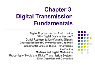
Chapter 3
Digital Transmission
Fundamentals
DigitalRepresentation of Information
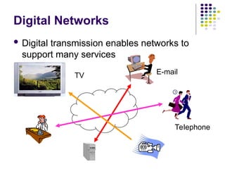
Why Digital Communications?
Digital Representation of Analog Signals
Characterization of Communication Channels
Fundamental Limits in Digital Transmission
Line Coding
Modems and Digital Modulation
Properties of Media and Digital Transmission Systems
Error Detection and Correction
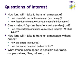
Questions of Interest
How long will it take to transmit a message?
How many bits are in the message (text, image)?
How fast does the network/system transfer information?
Can a network/system handle a voice (video) call?
How many bits/second does voice/video require? At what
quality?
How long will it take to transmit a message without
errors?
How are errors introduced?
How are errors detected and corrected?
What transmission speed is possible over radio,
copper cables, fiber, infrared, …?
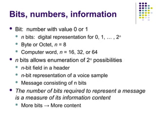
Bits, numbers, information
Bit: number with value 0 or 1
n bits: digital representation for 0, 1, … , 2n
Byte or Octet, n = 8
Computer word, n = 16, 32, or 64
n bits allows enumeration of 2n
possibilities
n-bit field in a header
n-bit representation of a voice sample
Message consisting of n bits
The number of bits required to represent a message
is a measure of its information content
More bits → More content
7.
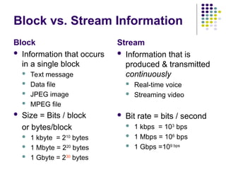
Block vs. StreamInformation
Block
Information that occurs
in a single block
Text message
Data file
JPEG image
MPEG file
Size = Bits / block
or bytes/block
1 kbyte = 210
bytes
1 Mbyte = 220
bytes
1 Gbyte = 230
bytes
Stream
Information that is
produced & transmitted
continuously
Real-time voice
Streaming video
Bit rate = bits / second
1 kbps = 103
bps
1 Mbps = 106
bps
1 Gbps =109 bps
8.
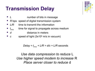
Transmission Delay
Use datacompression to reduce L
Use higher speed modem to increase R
Place server closer to reduce d
L number of bits in message
R bps speed of digital transmission system
L/R time to transmit the information
tprop time for signal to propagate across medium
d distance in meters
c speed of light (3x10⁸
m/s in vacuum)
Delay = tprop + L/R = d/c + L/R seconds
9.
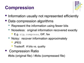
Compression
Information usuallynot represented efficiently
Data compression algorithms
Represent the information using fewer bits
Noiseless: original information recovered exactly
E.g. zip, compress, GIF, fax
Noisy: recover information approximately
JPEG
Tradeoff: # bits vs. quality
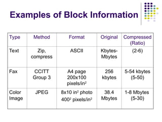
Compression Ratio
#bits (original file) / #bits (compressed file)
Type Method FormatOriginal Compressed
(Ratio)
Text Zip,
compress
ASCII Kbytes-
Mbytes
(2-6)
Fax CCITT
Group 3
A4 page
200x100
pixels/in2
256
kbytes
5-54 kbytes
(5-50)
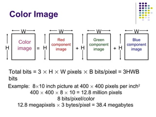
Color
Image
JPEG 8x10 in2
photo
4002
pixels/in2
38.4
Mbytes
1-8 Mbytes
(5-30)
Examples of Block Information
12.
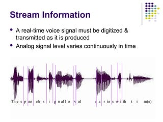
Th e sp ee ch s i g n al l e v el v a r ie s w i th t i m(e)
Stream Information
A real-time voice signal must be digitized &
transmitted as it is produced
Analog signal level varies continuously in time
13.
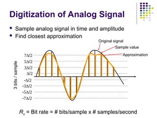
Digitization of AnalogSignal
Sample analog signal in time and amplitude
Find closest approximation
Original signal
Sample value
Approximation
Rs = Bit rate = # bits/sample x # samples/second
3
bits
/
sample
14.
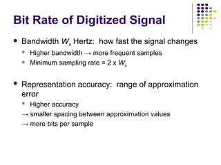
Bit Rate ofDigitized Signal
Bandwidth Ws Hertz: how fast the signal changes
Higher bandwidth → more frequent samples
Minimum sampling rate = 2 x Ws
Representation accuracy: range of approximation
error
Higher accuracy
→ smaller spacing between approximation values
→ more bits per sample
15.
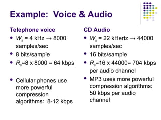
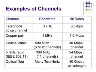
Example: Voice &Audio
Telephone voice
Ws = 4 kHz → 8000
samples/sec
8 bits/sample
Rs=8 x 8000 = 64 kbps
Cellular phones use
more powerful
compression
algorithms: 8-12 kbps
CD Audio
Ws = 22 kHertz → 44000
samples/sec
16 bits/sample
Rs=16 x 44000= 704 kbps
per audio channel
MP3 uses more powerful
compression algorithms:
50 kbps per audio
channel
16.
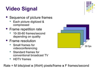
Video Signal
Sequenceof picture frames
Each picture digitized &
compressed
Frame repetition rate
10-30-60 frames/second
depending on quality
Frame resolution
Small frames for
videoconferencing
Standard frames for
conventional broadcast TV
HDTV frames
30 fps
Rate = M bits/pixel x (WxH) pixels/frame x F frames/second
17.
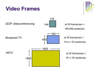
Video Frames
Broadcast TVat 30 frames/sec =
10.4 x 10⁶
pixels/sec
720
480
HDTV at 30 frames/sec =
67 x 106
pixels/sec
1080
1920
QCIF videoconferencing at 30 frames/sec =
760,000 pixels/sec
144
176
18.
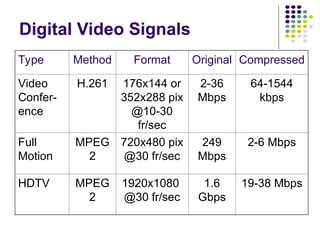
Digital Video Signals
TypeMethod Format Original Compressed
Video
Confer-
ence
H.261 176x144 or
352x288 pix
@10-30
fr/sec
2-36
Mbps
64-1544
kbps
Full
Motion
MPEG
2
720x480 pix
@30 fr/sec
249
Mbps
2-6 Mbps
HDTV MPEG
2
1920x1080
@30 fr/sec
1.6
Gbps
19-38 Mbps
19.
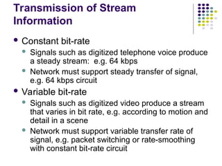
Transmission of Stream
Information
Constant bit-rate
Signals such as digitized telephone voice produce
a steady stream: e.g. 64 kbps
Network must support steady transfer of signal,
e.g. 64 kbps circuit
Variable bit-rate
Signals such as digitized video produce a stream
that varies in bit rate, e.g. according to motion and
detail in a scene
Network must support variable transfer rate of
signal, e.g. packet switching or rate-smoothing
with constant bit-rate circuit
20.
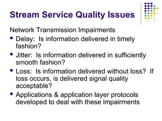
Stream Service QualityIssues
Network Transmission Impairments
Delay: Is information delivered in timely
fashion?
Jitter: Is information delivered in sufficiently
smooth fashion?
Loss: Is information delivered without loss? If
loss occurs, is delivered signal quality
acceptable?
Applications & application layer protocols
developed to deal with these impairments
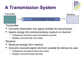
A Transmission System
Transmitter
Converts information into signal suitable for transmission
Injects energy into communications medium or channel
Telephone converts voice into electric current
Modem converts bits into tones
Receiver
Receives energy from medium
Converts received signal into form suitable for delivery to user
Telephone converts current into voice
Modem converts tones into bits
Receiver
Communication channel
Transmitter
23.
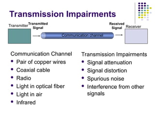
Transmission Impairments
Communication Channel
Pair of copper wires
Coaxial cable
Radio
Light in optical fiber
Light in air
Infrared
Transmission Impairments
Signal attenuation
Signal distortion
Spurious noise
Interference from other
signals
Transmitted
Signal
Received
Signal Receiver
Communication channel
Transmitter
24.
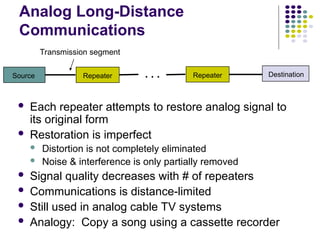
Analog Long-Distance
Communications
Eachrepeater attempts to restore analog signal to
its original form
Restoration is imperfect
Distortion is not completely eliminated
Noise & interference is only partially removed
Signal quality decreases with # of repeaters
Communications is distance-limited
Still used in analog cable TV systems
Analogy: Copy a song using a cassette recorder
Source Destination
Repeater
Transmission segment
Repeater
. . .
25.
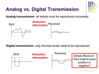
Analog vs. DigitalTransmission
Analog transmission: all details must be reproduced accurately
Sent
Sent
Received
Received
Distortion
Attenuation
Digital transmission: only discrete levels need to be reproduced
Distortion
Attenuation
Simple Receiver:
Was original pulse
positive or
negative?
26.
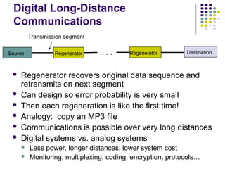
Digital Long-Distance
Communications
Regeneratorrecovers original data sequence and
retransmits on next segment
Can design so error probability is very small
Then each regeneration is like the first time!
Analogy: copy an MP3 file
Communications is possible over very long distances
Digital systems vs. analog systems
Less power, longer distances, lower system cost
Monitoring, multiplexing, coding, encryption, protocols…
Source Destination
Regenerator
Transmission segment
Regenerator
. . .
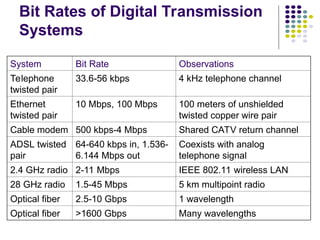
27.
Bit Rates ofDigital Transmission
Systems
System Bit Rate Observations
Telephone
twisted pair
33.6-56 kbps 4 kHz telephone channel
Ethernet
twisted pair
10 Mbps, 100 Mbps 100 meters of unshielded
twisted copper wire pair
Cable modem 500 kbps-4 Mbps Shared CATV return channel
ADSL twisted
pair
64-640 kbps in, 1.536-
6.144 Mbps out
Coexists with analog
telephone signal
2.4 GHz radio 2-11 Mbps IEEE 802.11 wireless LAN
28 GHz radio 1.5-45 Mbps 5 km multipoint radio
Optical fiber 2.5-10 Gbps 1 wavelength
Optical fiber >1600 Gbps Many wavelengths
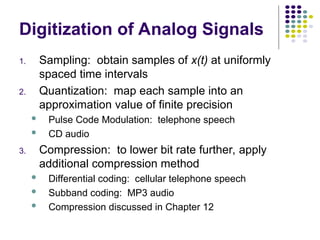
Digitization of AnalogSignals
1. Sampling: obtain samples of x(t) at uniformly
spaced time intervals
2. Quantization: map each sample into an
approximation value of finite precision
Pulse Code Modulation: telephone speech
CD audio
3. Compression: to lower bit rate further, apply
additional compression method
Differential coding: cellular telephone speech
Subband coding: MP3 audio
Compression discussed in Chapter 12
31.
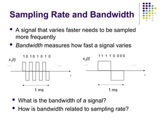
Sampling Rate andBandwidth
A signal that varies faster needs to be sampled
more frequently
Bandwidth measures how fast a signal varies
What is the bandwidth of a signal?
How is bandwidth related to sampling rate?
1 ms
1 1 1 1 0 0 0 0
. . . . . .
t
x2(t)
1 0 1 0 1 0 1 0
. . . . . .
t
1 ms
x1(t)
32.
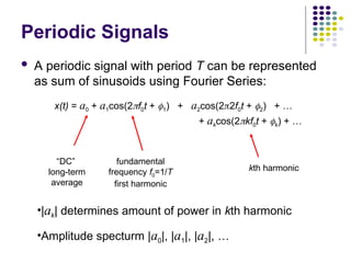
Periodic Signals
Aperiodic signal with period T can be represented
as sum of sinusoids using Fourier Series:
“DC”
long-term
average
fundamental
frequency f0=1/T
first harmonic
kth harmonic
x(t) = a0 + a1cos(2f0t + 1) + a2cos(22f0t + 2) + …
+ akcos(2kf0t + k) + …
•|ak| determines amount of power in kth harmonic
•Amplitude specturm |a0|, |a1|, |a2|, …
33.
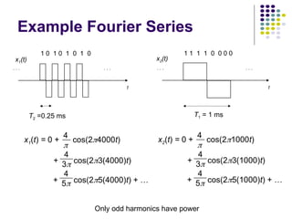
Example Fourier Series
T1= 1 ms
1 1 1 1 0 0 0 0
. . . . . .
t
x2(t)
1 0 1 0 1 0 1 0
. . . . . .
t
T2 =0.25 ms
x1(t)
Only odd harmonics have power
x1(t) = 0 + cos(24000t)
+ cos(23(4000)t)
+ cos(25(4000)t) + …
4
4
5
4
3
x2(t) = 0 + cos(21000t)
+ cos(23(1000)t)
+ cos(25(1000)t) + …
4
4
5
4
3
34.
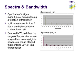
Spectra & Bandwidth
Spectrum of a signal:
magnitude of amplitudes as
a function of frequency
x1(t) varies faster in time &
has more high frequency
content than x2(t)
Bandwidth Ws is defined as
range of frequencies where
a signal has non-negligible
power, e.g. range of band
that contains 99% of total
signal power
0
0.2
0.4
0.6
0.8
1
1.2
0 3 6 9 12 15 18 21 24 27 30 33 36 39 42
frequency (kHz)
0
0.2
0.4
0.6
0.8
1
1.2
0 3 6 9 12 15 18 21 24 27 30 33 36 39 42
frequency (kHz)
Spectrum of x1(t)
Spectrum of x2(t)
35.
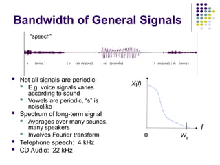
Bandwidth of GeneralSignals
Not all signals are periodic
E.g. voice signals varies
according to sound
Vowels are periodic, “s” is
noiselike
Spectrum of long-term signal
Averages over many sounds,
many speakers
Involves Fourier transform
Telephone speech: 4 kHz
CD Audio: 22 kHz
s (noisy ) | p (air stopped) | ee (periodic) | t (stopped) | sh (noisy)
X(f)
f
0 Ws
“speech”
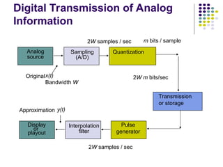
Digital Transmission ofAnalog
Information
Interpolation
filter
Display
or
playout
2W samples / sec
2W m bits/sec
x(t)
Bandwidth W
Sampling
(A/D)
Quantization
Analog
source
2W samples / sec m bits / sample
Pulse
generator
y(t)
Original
Approximation
Transmission
or storage
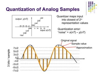
38.
input x(nT)
output y(nT)
Quantization error:
“noise” = x(nT) – y(nT)
Quantizer maps input
into closest of 2m
representation values
/2
3/2
5/2
7/2
-/2
-3/2
-5/2
-7/2
Original signal
Sample value
Approximation
3
bits
/
sample
Quantization of Analog Samples
39.
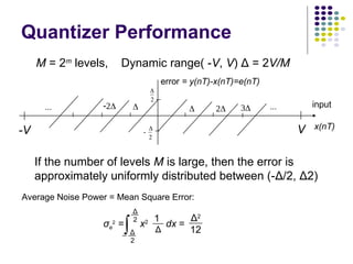
M = 2m
levels,Dynamic range( -V, V) Δ = 2V/M
Average Noise Power = Mean Square Error:
If the number of levels M is large, then the error is
approximately uniformly distributed between (-Δ/2, Δ2)
2
...
error = y(nT)-x(nT)=e(nT)
input
...
2
x(nT)
V
-V
Quantizer Performance
σe
2
= x2
dx =
Δ2
12
1
Δ
∫
Δ
2
Δ
2
40.
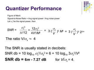
Figure of Merit:
Signal-to-NoiseRatio = Avg signal power / Avg noise power
Let x
2
be the signal power, then
x
2
/12
= 12x
2
4V2
/M2
=
x
3 (
V
)2
M2
= 3 (
V
)2
22m
x
SNR =
The ratio V/x 4
The SNR is usually stated in decibels:
SNR db = 10 log10 x
2
/e
2
= 6 + 10 log10 3x
2
/V2
SNR db = 6m - 7.27 dB for V/x = 4.
Quantizer Performance
41.
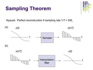
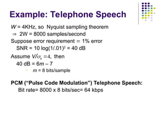
W = 4KHz,so Nyquist sampling theorem
2W = 8000 samples/second
Suppose error requirement 1% error
SNR = 10 log(1/.01)2
= 40 dB
Assume V/x then
40 dB = 6m – 7
m = 8 bits/sample
PCM (“Pulse Code Modulation”) Telephone Speech:
Bit rate= 8000 x 8 bits/sec= 64 kbps
Example: Telephone Speech
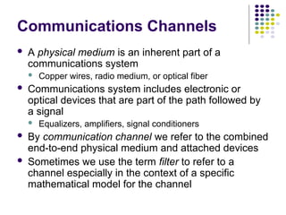
Communications Channels
Aphysical medium is an inherent part of a
communications system
Copper wires, radio medium, or optical fiber
Communications system includes electronic or
optical devices that are part of the path followed by
a signal
Equalizers, amplifiers, signal conditioners
By communication channel we refer to the combined
end-to-end physical medium and attached devices
Sometimes we use the term filter to refer to a
channel especially in the context of a specific
mathematical model for the channel
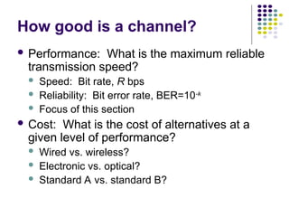
44.
How good isa channel?
Performance: What is the maximum reliable
transmission speed?
Speed: Bit rate, R bps
Reliability: Bit error rate, BER=10-k
Focus of this section
Cost: What is the cost of alternatives at a
given level of performance?
Wired vs. wireless?
Electronic vs. optical?
Standard A vs. standard B?
45.
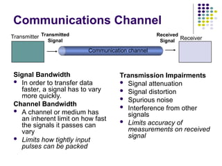
Communications Channel
Signal Bandwidth
In order to transfer data
faster, a signal has to vary
more quickly.
Channel Bandwidth
A channel or medium has
an inherent limit on how fast
the signals it passes can
vary
Limits how tightly input
pulses can be packed
Transmission Impairments
Signal attenuation
Signal distortion
Spurious noise
Interference from other
signals
Limits accuracy of
measurements on received
signal
Transmitted
Signal
Received
Signal Receiver
Communication channel
Transmitter
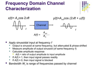
46.
Channel
t t
x(t)= Aincos2ft y(t)=Aoutcos (2ft + (f))
Aout
Ain
A(f) =
Frequency Domain Channel
Characterization
Apply sinusoidal input at frequency f
Output is sinusoid at same frequency, but attenuated & phase-shifted
Measure amplitude of output sinusoid (of same frequency f)
Calculate amplitude response
A(f) = ratio of output amplitude to input amplitude
If A(f) ≈ 1, then input signal passes readily
If A(f) ≈ 0, then input signal is blocked
Bandwidth Wc is range of frequencies passed by channel
47.
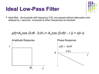
Ideal Low-Pass Filter
Ideal filter: all sinusoids with frequency f<Wc are passed without attenuation and
delayed by seconds; sinusoids at other frequencies are blocked
Amplitude Response
f
1
f
0
(f) = -2f
1/ 2
Phase Response
Wc
y(t)=Aincos (2ft - 2f )= Aincos (2f(t - )) = x(t-)
48.
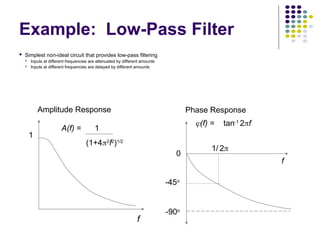
Example: Low-Pass Filter
Simplest non-ideal circuit that provides low-pass filtering
Inputs at different frequencies are attenuated by different amounts
Inputs at different frequencies are delayed by different amounts
f
1
A(f) = 1
(1+42
f2
)1/2
Amplitude Response
f
0
(f) = tan-1
2f
-45o
-90o
1/ 2
Phase Response
49.
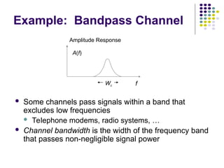
Example: Bandpass Channel
Some channels pass signals within a band that
excludes low frequencies
Telephone modems, radio systems, …
Channel bandwidth is the width of the frequency band
that passes non-negligible signal power
f
Amplitude Response
A(f)
Wc
50.
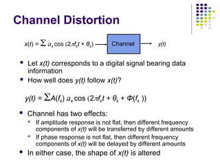
Channel Distortion
Channelhas two effects:
If amplitude response is not flat, then different frequency
components of x(t) will be transferred by different amounts
If phase response is not flat, then different frequency
components of x(t) will be delayed by different amounts
In either case, the shape of x(t) is altered
Let x(t) corresponds to a digital signal bearing data
information
How well does y(t) follow x(t)?
y(t) = A(fk) ak cos (2fkt + θk + Φ(fk ))
Channel y(t)
x(t) = ak cos (2fkt + θk)
51.
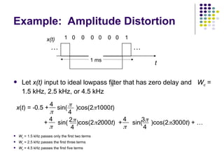
Example: Amplitude Distortion
Let x(t) input to ideal lowpass filter that has zero delay and Wc =
1.5 kHz, 2.5 kHz, or 4.5 kHz
1 0 0 0 0 0 0 1
. . . . . .
t
1 ms
x(t)
Wc = 1.5 kHz passes only the first two terms
Wc = 2.5 kHz passes the first three terms
Wc = 4.5 kHz passes the first five terms
x(t) = -0.5 + sin( )cos(21000t)
+ sin( )cos(22000t) + sin( )cos(23000t) + …
4
4
4
4
2
4
3
4
52.
- 1 .5
- 1
- 0 . 5
0
0 . 5
1
1 . 5
0
0
.
1
2
5
0
.
2
5
0
.
3
7
5
0
.
5
0
.
6
2
5
0
.
7
5
0
.
8
7
5
1
- 1 . 5
- 1
- 0 . 5
0
0 . 5
1
1 . 5
0
0
.
1
2
5
0
.
2
5
0
.
3
7
5
0
.
5
0
.
6
2
5
0
.
7
5
0
.
8
7
5
1
- 1 . 5
- 1
- 0 . 5
0
0 . 5
1
1 . 5
0
0
.
1
2
5
0
.
2
5
0
.
3
7
5
0
.
5
0
.
6
2
5
0
.
7
5
0
.
8
7
5
1
( b ) 2 H a r m o n i c s
( c ) 4 H a r m o n i c s
( a ) 1 H a r m o n i c
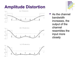
Amplitude Distortion
As the channel
bandwidth
increases, the
output of the
channel
resembles the
input more
closely
53.
Channel
t
0
t
h(t)
td
Time-domain Characterization
Time-domaincharacterization of a channel requires
finding the impulse response h(t)
Apply a very narrow pulse to a channel and observe
the channel output
h(t) typically a delayed pulse with ringing
Interested in system designs with h(t) that can be
packed closely without interfering with each other
54.
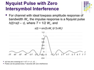
Nyquist Pulse withZero
Intersymbol Interference
For channel with ideal lowpass amplitude response of
bandwidth Wc, the impulse response is a Nyquist pulse
h(t)=s(t – ), where T = 1/2 Wc, and
-0.4
-0.2
0
0.2
0.4
0.6
0.8
1
1.2
-7 -6 -5 -4 -3 -2 -1 0 1 2 3 4 5 6 7
t
s(t) = sin(2Wc t)/ 2Wct
T T T T T T T T T T T T T T
s(t) has zero crossings at t = kT, k = +1, +2, …
Pulses can be packed every T seconds with zero interference
55.
-2
-1
0
1
2
-2 -1 01 2 3 4
t
T T T T T
T
-1
0
1
-2 -1 0 1 2 3 4
t
T T T T T
T
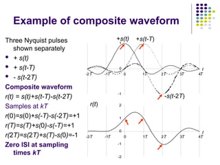
Example of composite waveform
Three Nyquist pulses
shown separately
+ s(t)
+ s(t-T)
- s(t-2T)
Composite waveform
r(t) = s(t)+s(t-T)-s(t-2T)
Samples at kT
r(0)=s(0)+s(-T)-s(-2T)=+1
r(T)=s(T)+s(0)-s(-T)=+1
r(2T)=s(2T)+s(T)-s(0)=-1
Zero ISI at sampling
times kT
r(t)
+s(t) +s(t-T)
-s(t-2T)
56.
0
f
A(f)
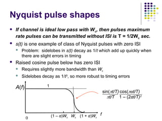
Nyquist pulse shapes
If channel is ideal low pass with Wc, then pulses maximum
rate pulses can be transmitted without ISI is T = 1/2Wc sec.
s(t) is one example of class of Nyquist pulses with zero ISI
Problem: sidelobes in s(t) decay as 1/t which add up quickly when
there are slight errors in timing
Raised cosine pulse below has zero ISI
Requires slightly more bandwidth than Wc
Sidelobes decay as 1/t3
, so more robust to timing errors
1
sin(t/T)
t/T
cos(αt/T)
1 – (2αt/T)2
(1 – α)Wc Wc (1 + α)Wc
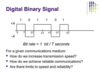
Digital Binary Signal
Fora given communications medium:
How do we increase transmission speed?
How do we achieve reliable communications?
Are there limits to speed and reliability?
+A
-A
0 T 2T 3T 4T 5T 6T
1 1 1 1
0 0
Bit rate = 1 bit / T seconds
59.
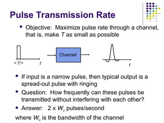
Pulse Transmission Rate
Objective: Maximize pulse rate through a channel,
that is, make T as small as possible
Channel
t t
If input is a narrow pulse, then typical output is a
spread-out pulse with ringing
Question: How frequently can these pulses be
transmitted without interfering with each other?
Answer: 2 x Wc pulses/second
where Wc is the bandwidth of the channel
T
60.
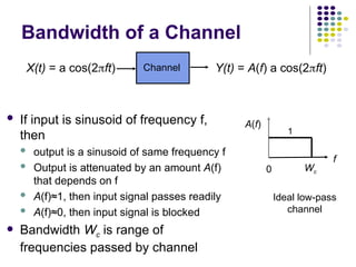
Bandwidth of aChannel
If input is sinusoid of frequency f,
then
output is a sinusoid of same frequency f
Output is attenuated by an amount A(f)
that depends on f
A(f)≈1, then input signal passes readily
A(f)≈0, then input signal is blocked
Bandwidth Wc is range of
frequencies passed by channel
Channel
X(t) = a cos(2ft) Y(t) = A(f) a cos(2ft)
Wc
0
f
A(f)
1
Ideal low-pass
channel
61.
Transmitter
Filter
Communication
Medium
Receiver
Filter Receiver
r(t)
Received signal
+A
-A
0T 2T 3T 4T 5T
1 1 1 1
0 0
t
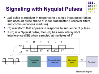
Signaling with Nyquist Pulses
p(t) pulse at receiver in response to a single input pulse (takes
into account pulse shape at input, transmitter & receiver filters,
and communications medium)
r(t) waveform that appears in response to sequence of pulses
If s(t) is a Nyquist pulse, then r(t) has zero intersymbol
interference (ISI) when sampled at multiples of T
62.
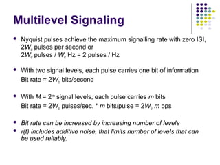
Multilevel Signaling
Nyquistpulses achieve the maximum signalling rate with zero ISI,
2Wc pulses per second or
2Wc pulses / Wc Hz = 2 pulses / Hz
With two signal levels, each pulse carries one bit of information
Bit rate = 2Wc bits/second
With M = 2m
signal levels, each pulse carries m bits
Bit rate = 2Wc pulses/sec. * m bits/pulse = 2Wc m bps
Bit rate can be increased by increasing number of levels
r(t) includes additive noise, that limits number of levels that can
be used reliably.
63.
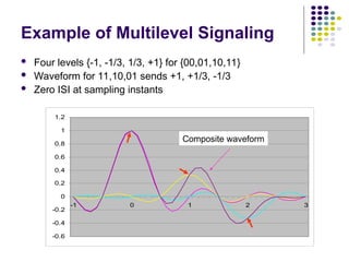
Example of MultilevelSignaling
Four levels {-1, -1/3, 1/3, +1} for {00,01,10,11}
Waveform for 11,10,01 sends +1, +1/3, -1/3
Zero ISI at sampling instants
-0.6
-0.4
-0.2
0
0.2
0.4
0.6
0.8
1
1.2
-1 0 1 2 3
Composite waveform
64.
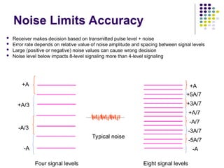
Four signal levelsEight signal levels
Typical noise
Noise Limits Accuracy
Receiver makes decision based on transmitted pulse level + noise
Error rate depends on relative value of noise amplitude and spacing between signal levels
Large (positive or negative) noise values can cause wrong decision
Noise level below impacts 8-level signaling more than 4-level signaling
+A
+A/3
-A/3
-A
+A
+5A/7
+3A/7
+A/7
-A/7
-3A/7
-5A/7
-A
65.
2
2
2
2
1
x
e
x
0
Noise distribution
Noise is characterized by probability density of amplitude samples
Likelihood that certain amplitude occurs
Thermal electronic noise is inevitable (due to vibrations of electrons)
Noise distribution is Gaussian (bell-shaped) as below
t
x
Pr[X(t)>x0 ] = ?
Pr[X(t)>x0 ] =
Area under
graph
x0
x0
= Avg Noise Power
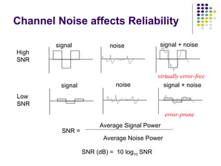
signal noise signal+ noise
signal noise signal + noise
High
SNR
Low
SNR
SNR =
Average Signal Power
Average Noise Power
SNR (dB) = 10 log10 SNR
virtually error-free
error-prone
Channel Noise affects Reliability
68.
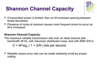
If transmittedpower is limited, then as M increases spacing between
levels decreases
Presence of noise at receiver causes more frequent errors to occur as
M is increased
Shannon Channel Capacity:
The maximum reliable transmission rate over an ideal channel with
bandwidth W Hz, with Gaussian distributed noise, and with SNR S/N is
C = W log2 ( 1 + S/N ) bits per second
Reliable means error rate can be made arbitrarily small by proper
coding
Shannon Channel Capacity
69.
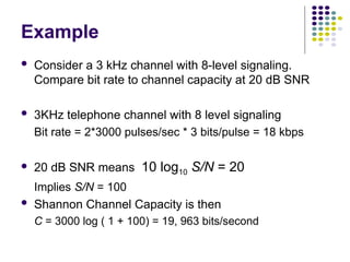
Example
Consider a3 kHz channel with 8-level signaling.
Compare bit rate to channel capacity at 20 dB SNR
3KHz telephone channel with 8 level signaling
Bit rate = 2*3000 pulses/sec * 3 bits/pulse = 18 kbps
20 dB SNR means 10 log10 S/N = 20
Implies S/N = 100
Shannon Channel Capacity is then
C = 3000 log ( 1 + 100) = 19, 963 bits/second
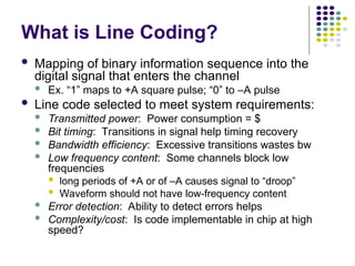
What is LineCoding?
Mapping of binary information sequence into the
digital signal that enters the channel
Ex. “1” maps to +A square pulse; “0” to –A pulse
Line code selected to meet system requirements:
Transmitted power: Power consumption = $
Bit timing: Transitions in signal help timing recovery
Bandwidth efficiency: Excessive transitions wastes bw
Low frequency content: Some channels block low
frequencies
long periods of +A or of –A causes signal to “droop”
Waveform should not have low-frequency content
Error detection: Ability to detect errors helps
Complexity/cost: Is code implementable in chip at high
speed?
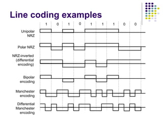
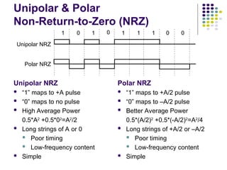
Unipolar & Polar
Non-Return-to-Zero(NRZ)
Unipolar NRZ
“1” maps to +A pulse
“0” maps to no pulse
High Average Power
0.5*A2
+0.5*02
=A2
/2
Long strings of A or 0
Poor timing
Low-frequency content
Simple
Polar NRZ
“1” maps to +A/2 pulse
“0” maps to –A/2 pulse
Better Average Power
0.5*(A/2)2
+0.5*(-A/2)2
=A2
/4
Long strings of +A/2 or –A/2
Poor timing
Low-frequency content
Simple
1 0 1 0 1 1 0 0
1
Unipolar NRZ
Polar NRZ
75.
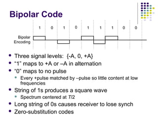
Bipolar Code
Threesignal levels: {-A, 0, +A}
“1” maps to +A or –A in alternation
“0” maps to no pulse
Every +pulse matched by –pulse so little content at low
frequencies
String of 1s produces a square wave
Spectrum centered at T/2
Long string of 0s causes receiver to lose synch
Zero-substitution codes
1 0 1 0 1 1 0 0
1
Bipolar
Encoding
76.
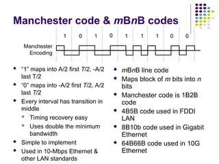
Manchester code &mBnB codes
“1” maps into A/2 first T/2, -A/2
last T/2
“0” maps into -A/2 first T/2, A/2
last T/2
Every interval has transition in
middle
Timing recovery easy
Uses double the minimum
bandwidth
Simple to implement
Used in 10-Mbps Ethernet &
other LAN standards
mBnB line code
Maps block of m bits into n
bits
Manchester code is 1B2B
code
4B5B code used in FDDI
LAN
8B10b code used in Gigabit
Ethernet
64B66B code used in 10G
Ethernet
1 0 1 0 1 1 0 0
1
Manchester
Encoding
77.
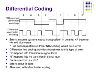
Differential Coding
Errorsin some systems cause transposition in polarity, +A become
–A and vice versa
All subsequent bits in Polar NRZ coding would be in error
Differential line coding provides robustness to this type of error
“1” mapped into transition in signal level
“0” mapped into no transition in signal level
Same spectrum as NRZ
Errors occur in pairs
Also used with Manchester coding
NRZ-inverted
(differential
encoding)
1 0 1 0 1 1 0 0
1
Differential
Manchester
encoding
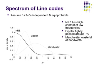
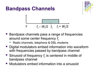
Bandpass Channels
Bandpasschannels pass a range of frequencies
around some center frequency fc
Radio channels, telephone & DSL modems
Digital modulators embed information into waveform
with frequencies passed by bandpass channel
Sinusoid of frequency fc is centered in middle of
bandpass channel
Modulators embed information into a sinusoid
fc – Wc/2 fc
0 fc + Wc/2
80.
Information 1 11 1
0 0
+1
-1
0 T 2T 3T 4T 5T 6T
Amplitude
Shift
Keying
+1
-1
Frequency
Shift
Keying 0 T 2T 3T 4T 5T 6T
t
t
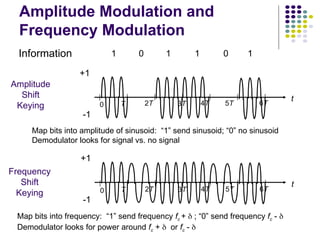
Amplitude Modulation and
Frequency Modulation
Map bits into amplitude of sinusoid: “1” send sinusoid; “0” no sinusoid
Demodulator looks for signal vs. no signal
Map bits into frequency: “1” send frequency fc + ; “0” send frequency fc -
Demodulator looks for power around fc + or fc -
81.
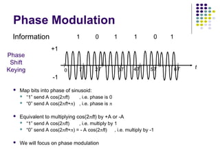
Phase Modulation
Mapbits into phase of sinusoid:
“1” send A cos(2ft) , i.e. phase is 0
“0” send A cos(2ft+) , i.e. phase is
Equivalent to multiplying cos(2ft) by +A or -A
“1” send A cos(2ft) , i.e. multiply by 1
“0” send A cos(2ft+) = - A cos(2ft) , i.e. multiply by -1
We will focus on phase modulation
+1
-1
Phase
Shift
Keying 0 T 2T 3T 4T 5T 6T t
Information 1 1 1 1
0 0
82.
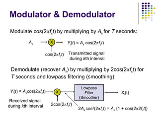
Modulate cos(2fct) bymultiplying by Ak for T seconds:
Ak
x
cos(2fct)
Yi(t) = Ak cos(2fct)
Transmitted signal
during kth interval
Demodulate (recover Ak) by multiplying by 2cos(2fct) for
T seconds and lowpass filtering (smoothing):
x
2cos(2fct)
2Ak cos2
(2fct) = Ak {1 + cos(22fct)}
Lowpass
Filter
(Smoother)
Xi(t)
Yi(t) = Akcos(2fct)
Received signal
during kth interval
Modulator & Demodulator
83.
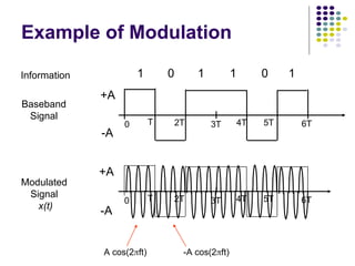
1 1 11
0 0
+A
-A
0 T 2T 3T 4T 5T 6T
Information
Baseband
Signal
Modulated
Signal
x(t)
+A
-A
0 T 2T 3T 4T 5T 6T
Example of Modulation
A cos(2ft) -A cos(2ft)
84.
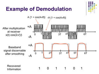
1 1 11
0 0
Recovered
Information
Baseband
signal discernable
after smoothing
After multiplication
at receiver
x(t) cos(2fct)
+A
-A
0 T 2T 3T 4T 5T 6T
+A
-A
0 T 2T 3T 4T 5T 6T
Example of Demodulation
A {1 + cos(4ft)} -A {1 + cos(4ft)}
85.
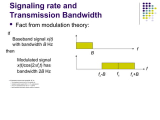
Signaling rate and
TransmissionBandwidth
Fact from modulation theory:
Baseband signal x(t)
with bandwidth B Hz
If
then B
fc+B
f
f
fc-B fc
Modulated signal
x(t)cos(2fct) has
bandwidth 2B Hz
If bandpass channel has bandwidth Wc Hz,
Then baseband channel has Wc/2 Hz available, so
modulation system supports Wc/2 x 2 = Wc pulses/second
That is, Wc pulses/second per Wc Hz = 1 pulse/Hz
Recall baseband transmission system supports 2 pulses/Hz
86.
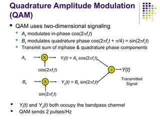
Ak
x
cos(2fct)
Yi(t) = Akcos(2fct)
Bk
x
sin(2fct)
Yq(t) = Bk sin(2fct)
+ Y(t)
Yi(t) and Yq(t) both occupy the bandpass channel
QAM sends 2 pulses/Hz
Quadrature Amplitude Modulation
(QAM)
QAM uses two-dimensional signaling
Ak modulates in-phase cos(2fct)
Bk modulates quadrature phase cos(2fct + /4) = sin(2fct)
Transmit sum of inphase & quadrature phase components
Transmitted
Signal
87.
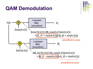
QAM Demodulation
Y(t) x
2cos(2fct)
2cos2
(2fct)+2Bkcos(2fct)sin(2fct)
= Ak {1 + cos(4fct)}+Bk {0 + sin(4fct)}
Lowpass
filter
(smoother)
Ak
2Bk sin2
(2fct)+2Ak cos(2fct)sin(2fct)
= Bk {1 - cos(4fct)}+Ak {0 + sin(4fct)}
x
2sin(2fct)
Bk
Lowpass
filter
(smoother)
smoothed to zero
smoothed to zero
88.
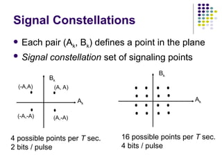
Signal Constellations
Eachpair (Ak, Bk) defines a point in the plane
Signal constellation set of signaling points
4 possible points per T sec.
2 bits / pulse
Ak
Bk
16 possible points per T sec.
4 bits / pulse
Ak
Bk
(A, A)
(A,-A)
(-A,-A)
(-A,A)
89.
Ak
Bk
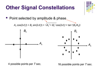
4 possible pointsper T sec.
Ak
Bk
16 possible points per T sec.
Other Signal Constellations
Point selected by amplitude & phase
Ak cos(2fct) + Bk sin(2fct) = √Ak
2
+ Bk
2
cos(2fct + tan-1
(Bk/Ak))
90.
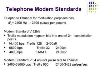
Telephone Modem Standards
TelephoneChannel for modulation purposes has
Wc = 2400 Hz → 2400 pulses per second
Modem Standard V.32bis
Trellis modulation maps m bits into one of 2m+1
constellation
points
14,400 bps Trellis 128 2400x6
9600 bps Trellis 32 2400x4
4800 bps QAM 4 2400x2
Modem Standard V.34 adjusts pulse rate to channel
2400-33600 bps Trellis 960 2400-3429 pulses/sec
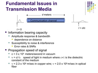
Fundamental Issues in
TransmissionMedia
Information bearing capacity
Amplitude response & bandwidth
dependence on distance
Susceptibility to noise & interference
Error rates & SNRs
Propagation speed of signal
c = 3 x 10⁸
meters/second in vacuum
= c/√speed of light in medium where is the dielectric
constant of the medium
= 2.3 x 10⁸
m/sec in copper wire; = 2.0 x 10⁸
m/sec in optical
fiber
t = 0
t = d/c
Communication channel
d meters
93.
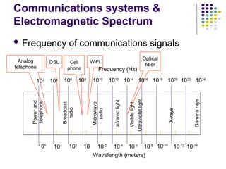
Communications systems &
ElectromagneticSpectrum
Frequency of communications signals
Analog
telephone
DSL Cell
phone
WiFi
Optical
fiber
102
104 106
108
1010
1012
1014
1016
1018
1020
1022
1024
Frequency (Hz)
Wavelength (meters)
106
104 102
10 10-2
10-4
10-6
10-8 10-10
10-12
10-14
Power
and
telephone
Broadcast
radio
Microwave
radio
Infrared
light
Visible
light
Ultraviolet
light
X-rays
Gamma
rays
94.
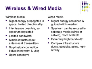
Wireless & WiredMedia
Wireless Media
Signal energy propagates in
space, limited directionality
Interference possible, so
spectrum regulated
Limited bandwidth
Simple infrastructure:
antennas & transmitters
No physical connection
between network & user
Users can move
Wired Media
Signal energy contained &
guided within medium
Spectrum can be re-used in
separate media (wires or
cables), more scalable
Extremely high bandwidth
Complex infrastructure:
ducts, conduits, poles, right-
of-way
95.
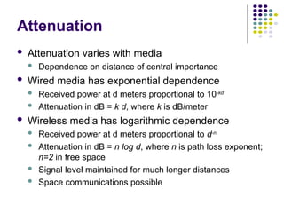
Attenuation
Attenuation varieswith media
Dependence on distance of central importance
Wired media has exponential dependence
Received power at d meters proportional to 10-kd
Attenuation in dB = k d, where k is dB/meter
Wireless media has logarithmic dependence
Received power at d meters proportional to d-n
Attenuation in dB = n log d, where n is path loss exponent;
n=2 in free space
Signal level maintained for much longer distances
Space communications possible
96.
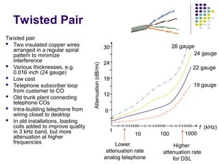
Twisted Pair
Twisted pair
Two insulated copper wires
arranged in a regular spiral
pattern to minimize
interference
Various thicknesses, e.g.
0.016 inch (24 gauge)
Low cost
Telephone subscriber loop
from customer to CO
Old trunk plant connecting
telephone COs
Intra-building telephone from
wiring closet to desktop
In old installations, loading
coils added to improve quality
in 3 kHz band, but more
attenuation at higher
frequencies
Attenuation
(dB/mi)
f (kHz)
19 gauge
22 gauge
24 gauge
26 gauge
6
12
18
24
30
1
10 100 1000
Lower
attenuation rate
analog telephone
Higher
attenuation rate
for DSL
97.
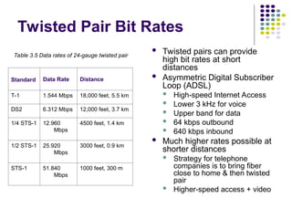
Twisted Pair BitRates
Twisted pairs can provide
high bit rates at short
distances
Asymmetric Digital Subscriber
Loop (ADSL)
High-speed Internet Access
Lower 3 kHz for voice
Upper band for data
64 kbps outbound
640 kbps inbound
Much higher rates possible at
shorter distances
Strategy for telephone
companies is to bring fiber
close to home & then twisted
pair
Higher-speed access + video
Table 3.5 Data rates of 24-gauge twisted pair
Standard Data Rate Distance
T-1 1.544 Mbps 18,000 feet, 5.5 km
DS2 6.312 Mbps 12,000 feet, 3.7 km
1/4 STS-1 12.960
Mbps
4500 feet, 1.4 km
1/2 STS-1 25.920
Mbps
3000 feet, 0.9 km
STS-1 51.840
Mbps
1000 feet, 300 m
98.
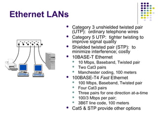
Ethernet LANs
Category3 unshielded twisted pair
(UTP): ordinary telephone wires
Category 5 UTP: tighter twisting to
improve signal quality
Shielded twisted pair (STP): to
minimize interference; costly
10BASE-T Ethernet
10 Mbps, Baseband, Twisted pair
Two Cat3 pairs
Manchester coding, 100 meters
100BASE-T4 Fast Ethernet
100 Mbps, Baseband, Twisted pair
Four Cat3 pairs
Three pairs for one direction at-a-time
100/3 Mbps per pair;
3B6T line code, 100 meters
Cat5 & STP provide other options
99.
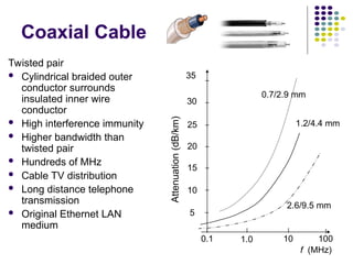
Coaxial Cable
Twisted pair
Cylindrical braided outer
conductor surrounds
insulated inner wire
conductor
High interference immunity
Higher bandwidth than
twisted pair
Hundreds of MHz
Cable TV distribution
Long distance telephone
transmission
Original Ethernet LAN
medium
35
30
10
25
20
5
15
Attenuation
(dB/km)
0.1 1.0 10 100
f (MHz)
2.6/9.5 mm
1.2/4.4 mm
0.7/2.9 mm
100.
Upstream
Downstream
5
MHz
42
MHz
54
MHz
500
MHz
550
MHz
750
MHz
Downstream
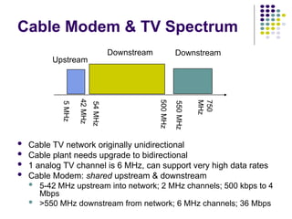
Cable Modem &TV Spectrum
Cable TV network originally unidirectional
Cable plant needs upgrade to bidirectional
1 analog TV channel is 6 MHz, can support very high data rates
Cable Modem: shared upstream & downstream
5-42 MHz upstream into network; 2 MHz channels; 500 kbps to 4
Mbps
>550 MHz downstream from network; 6 MHz channels; 36 Mbps
101.
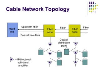
Cable Network Topology
Head
end
Upstreamfiber
Downstream fiber
Fiber
node
Coaxial
distribution
plant
Fiber
node
= Bidirectional
split-band
amplifier
Fiber Fiber
102.
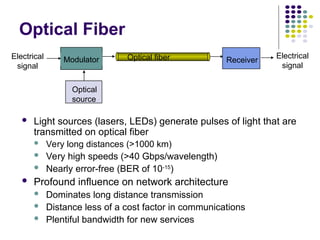
Optical Fiber
Lightsources (lasers, LEDs) generate pulses of light that are
transmitted on optical fiber
Very long distances (>1000 km)
Very high speeds (>40 Gbps/wavelength)
Nearly error-free (BER of 10-15
)
Profound influence on network architecture
Dominates long distance transmission
Distance less of a cost factor in communications
Plentiful bandwidth for new services
Optical fiber
Optical
source
Modulator
Electrical
signal
Receiver
Electrical
signal
103.
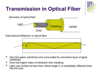
Core
Cladding Jacket
Light
c
Geometry ofoptical fiber
Total Internal Reflection in optical fiber
Transmission in Optical Fiber
Very fine glass cylindrical core surrounded by concentric layer of glass
(cladding)
Core has higher index of refraction than cladding
Light rays incident at less than critical angle c is completely reflected back
into the core
104.
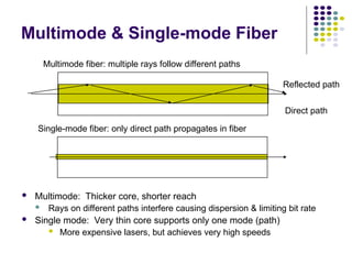
Multimode: Thickercore, shorter reach
Rays on different paths interfere causing dispersion & limiting bit rate
Single mode: Very thin core supports only one mode (path)
More expensive lasers, but achieves very high speeds
Multimode fiber: multiple rays follow different paths
Single-mode fiber: only direct path propagates in fiber
Direct path
Reflected path
Multimode & Single-mode Fiber
105.
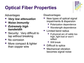
Optical Fiber Properties
Advantages
Very low attenuation
Noise immunity
Extremely high
bandwidth
Security: Very difficult to
tap without breaking
No corrosion
More compact & lighter
than copper wire
Disadvantages
New types of optical signal
impairments & dispersion
Polarization dependence
Wavelength dependence
Limited bend radius
If physical arc of cable too
high, light lost or won’t
reflect
Will break
Difficult to splice
Mechanical vibration
becomes signal noise
106.
100
50
10
5
1
0.5
0.1
0.05
0.01
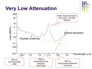
0.8 1.0 1.21.4 1.6 1.8 Wavelength (m)
Loss
(dB/km)
Infrared absorption
Rayleigh scattering
Very Low Attenuation
850 nm
Low-cost LEDs
LANs
1300 nm
Metropolitan Area
Networks
“Short Haul”
1550 nm
Long Distance Networks
“Long Haul
Water Vapor Absorption
(removed in new fiber
designs)
107.
100
50
10
5
1
0.5
0.1
0.8 1.0 1.21.4 1.6 1.8
Loss
(dB/km)
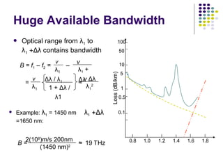
Huge Available Bandwidth
Optical range from λ1to
λ1Δλ contains bandwidth
Example: λ1= 1450 nm λ1Δλ
=1650 nm:
B = ≈ 19 THz
B = f1 – f2 = –
v
λ1 +
Δλ
v
λ1
v Δλ
λ1
2
= ≈
Δλ / λ1
1 + Δλ /
λ1
v
λ1
2(108
)m/s 200nm
(1450 nm)2
108.
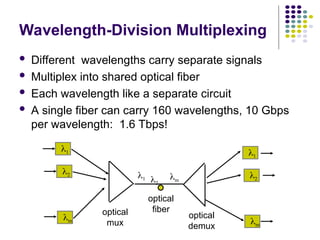
Wavelength-Division Multiplexing
Differentwavelengths carry separate signals
Multiplex into shared optical fiber
Each wavelength like a separate circuit
A single fiber can carry 160 wavelengths, 10 Gbps
per wavelength: 1.6 Tbps!
1
2
m
optical
mux
1
2
m
optical
demux
1 2.
m
optical
fiber
109.
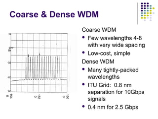
Coarse & DenseWDM
Coarse WDM
Few wavelengths 4-8
with very wide spacing
Low-cost, simple
Dense WDM
Many tightly-packed
wavelengths
ITU Grid: 0.8 nm
separation for 10Gbps
signals
0.4 nm for 2.5 Gbps
155
0
156
0
154
0
110.
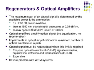
Regenerators & OpticalAmplifiers
The maximum span of an optical signal is determined by the
available power & the attenuation:
Ex. If 30 dB power available,
then at 1550 nm, optical signal attenuates at 0.25 dB/km,
so max span = 30 dB/0.25 km/dB = 120 km
Optical amplifiers amplify optical signal (no equalization, no
regeneration)
Impairments in optical amplification limit maximum number of
optical amplifiers in a path
Optical signal must be regenerated when this limit is reached
Requires optical-to-electrical (O-to-E) signal conversion,
equalization, detection and retransmission (E-to-O)
Expensive
Severe problem with WDM systems
111.
Regenerator
R R RR R R R R
DWDM
multiplexer
… …
R
R
R
R
…
R
R
R
R
…
R
R
R
R
…
R
R
R
R
…
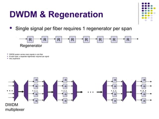
DWDM & Regeneration
Single signal per fiber requires 1 regenerator per span
DWDM system carries many signals in one fiber
At each span, a separate regenerator required per signal
Very expensive
112.
R
R
R
R
Optical
amplifier
… … …
R
R
R
R
OAOA OA OA
… …
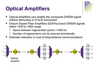
Optical Amplifiers
Optical amplifiers can amplify the composite DWDM signal
without demuxing or O-to-E conversion
Erbium Doped Fiber Amplifiers (EDFAs) boost DWDM signals
within 1530 to 1620 range
Spans between regeneration points >1000 km
Number of regenerators can be reduced dramatically
Dramatic reduction in cost of long-distance communications
113.
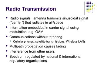
Radio Transmission
Radiosignals: antenna transmits sinusoidal signal
(“carrier”) that radiates in air/space
Information embedded in carrier signal using
modulation, e.g. QAM
Communications without tethering
Cellular phones, satellite transmissions, Wireless LANs
Multipath propagation causes fading
Interference from other users
Spectrum regulated by national & international
regulatory organizations
114.
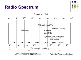
104 106
107
108
109
1010 10111012
Frequency (Hz)
Wavelength (meters)
103 102
101 1 10-1
10-2 10-3
105
Satellite and terrestrial
microwave
AM radio
FM radio and TV
LF MF HF VHF UHF SHF EHF
10
4
Cellular
and PCS
Wireless cable
Radio Spectrum
Omni-directional applications Point-to-Point applications
115.
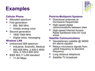
Examples
Cellular Phone
Allocatedspectrum
First generation:
800, 900 MHz
Initially analog voice
Second generation:
1800-1900 MHz
Digital voice, messaging
Wireless LAN
Unlicenced ISM spectrum
Industrial, Scientific, Medical
902-928 MHz, 2.400-2.4835
GHz, 5.725-5.850 GHz
IEEE 802.11 LAN standard
11-54 Mbps
Point-to-Multipoint Systems
Directional antennas at
microwave frequencies
High-speed digital
communications between sites
High-speed Internet Access
Radio backbone links for rural
areas
Satellite Communications
Geostationary satellite @ 36000
km above equator
Relays microwave signals from
uplink frequency to downlink
frequency
Long distance telephone
Satellite TV broadcast
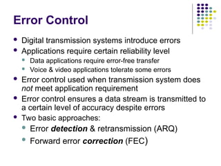
Error Control
Digitaltransmission systems introduce errors
Applications require certain reliability level
Data applications require error-free transfer
Voice & video applications tolerate some errors
Error control used when transmission system does
not meet application requirement
Error control ensures a data stream is transmitted to
a certain level of accuracy despite errors
Two basic approaches:
Error detection & retransmission (ARQ)
Forward error correction (FEC)
118.
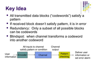
Key Idea
Alltransmitted data blocks (“codewords”) satisfy a
pattern
If received block doesn’t satisfy pattern, it is in error
Redundancy: Only a subset of all possible blocks
can be codewords
Blindspot: when channel transforms a codeword
into another codeword
Channel
Encoder
User
information
Pattern
checking
All inputs to channel
satisfy pattern or condition
Channel
output
Deliver user
information or
set error alarm
119.
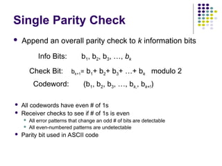
Single Parity Check
Append an overall parity check to k information bits
Info Bits: b1, b2, b3, …, bk
Check Bit: bk+1= b1+ b2+ b3+ …+ bk modulo 2
Codeword: (b1, b2, b3, …, bk,, bk+!)
All codewords have even # of 1s
Receiver checks to see if # of 1s is even
All error patterns that change an odd # of bits are detectable
All even-numbered patterns are undetectable
Parity bit used in ASCII code
120.
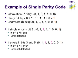
Example of SingleParity Code
Information (7 bits): (0, 1, 0, 1, 1, 0, 0)
Parity Bit: b8 = 0 + 1 +0 + 1 +1 + 0 = 1
Codeword (8 bits): (0, 1, 0, 1, 1, 0, 0, 1)
If single error in bit 3 : (0, 1, 1, 1, 1, 0, 0, 1)
# of 1’s =5, odd
Error detected
If errors in bits 3 and 5: (0, 1, 1, 1, 0, 0, 0, 1)
# of 1’s =4, even
Error not detected
121.
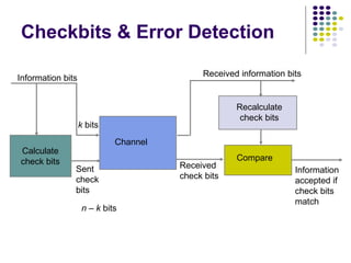
Checkbits & ErrorDetection
Calculate
check bits
Channel
Recalculate
check bits
Compare
Information bits Received information bits
Sent
check
bits
Information
accepted if
check bits
match
Received
check bits
k bits
n – k bits
122.
How good isthe single parity
check code?
Redundancy: Single parity check code adds 1
redundant bit per k information bits:
overhead = 1/(k + 1)
Coverage: all error patterns with odd # of errors can
be detected
An error patten is a binary (k + 1)-tuple with 1s where
errors occur and 0’s elsewhere
Of 2k+1
binary (k + 1)-tuples, ½ are odd, so 50% of error
patterns can be detected
Is it possible to detect more errors if we add more
check bits?
Yes, with the right codes
123.
What if biterrors are random?
Many transmission channels introduce bit errors at random,
independently of each other, and with probability p
Some error patterns are more probable than others:
In any worthwhile channel p < 0.5, and so p/(1 – p) < 1
It follows that patterns with 1 error are more likely than patterns with 2 errors and so
forth
What is the probability that an undetectable error pattern occurs?
P[10000000] = p(1 – p)7
and
P[11000000] = p2
(1 – p)6
124.
Single parity checkcode with
random bit errors
Undetectable error pattern if even # of bit errors:
Example: Evaluate above for n = 32, p = 10-3
For this example, roughly 1 in 2000 error patterns is undetectable
P[error detection failure] = P[undetectable error pattern]
= P[error patterns with even number of 1s]
= p2
(1 – p)n-2
+ p4
(1 – p)n-4
+ …
n
2
n
4
P[undetectable error] = (10-3
)2
(1 – 10-3
)30
+ (10-3
)4
(1 – 10-3
)28
≈ 496 (10-6
) + 35960 (10-12
) ≈ 4.96 (10-4
)
32
2
32
4
125.
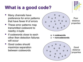
x = codewords
o= noncodewords
x
x x
x
x
x
x
o
o
o
o
o
o
o
o
o
o
o
o
o
x
x x
x
x
x
x
o
o
o
o
o
o
o
o
o
o
o Poor
distance
properties
What is a good code?
Many channels have
preference for error patterns
that have fewer # of errors
These error patterns map
transmitted codeword to
nearby n-tuple
If codewords close to each
other then detection failures
will occur
Good codes should
maximize separation
between codewords
Good
distance
properties
126.
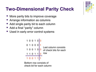
Two-Dimensional Parity Check
10 0 1 0 0
0 1 0 0 0 1
1 0 0 1 0 0
1 1 0 1 1 0
1 0 0 1 1 1
Bottom row consists of
check bit for each column
Last column consists
of check bits for each
row
More parity bits to improve coverage
Arrange information as columns
Add single parity bit to each column
Add a final “parity” column
Used in early error control systems
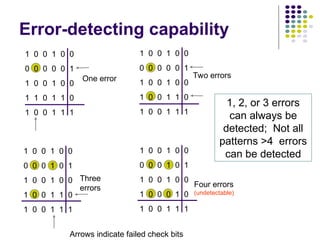
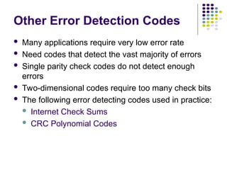
Other Error DetectionCodes
Many applications require very low error rate
Need codes that detect the vast majority of errors
Single parity check codes do not detect enough
errors
Two-dimensional codes require too many check bits
The following error detecting codes used in practice:
Internet Check Sums
CRC Polynomial Codes
129.
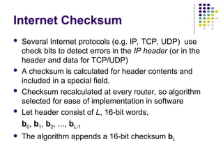
Internet Checksum
SeveralInternet protocols (e.g. IP, TCP, UDP) use
check bits to detect errors in the IP header (or in the
header and data for TCP/UDP)
A checksum is calculated for header contents and
included in a special field.
Checksum recalculated at every router, so algorithm
selected for ease of implementation in software
Let header consist of L, 16-bit words,
b0, b1, b2, ..., bL-1
The algorithm appends a 16-bit checksum bL
130.
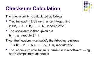
The checksum bLis calculated as follows:
Treating each 16-bit word as an integer, find
x = b0 + b1 + b2+ ...+ bL-1 modulo 216
-1
The checksum is then given by:
bL = - x modulo 216
-1
Thus, the headers must satisfy the following pattern:
0 = b0 + b1 + b2+ ...+ bL-1 + bL modulo 216
-1
The checksum calculation is carried out in software using
one’s complement arithmetic
Checksum Calculation
131.
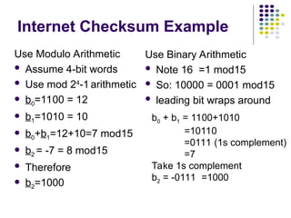
Internet Checksum Example
UseModulo Arithmetic
Assume 4-bit words
Use mod 24
-1 arithmetic
b0=1100 = 12
b1=1010 = 10
b0+b1=12+10=7 mod15
b2 = -7 = 8 mod15
Therefore
b2=1000
Use Binary Arithmetic
Note 16 =1 mod15
So: 10000 = 0001 mod15
leading bit wraps around
b0 + b1 = 1100+1010
=10110
=0111 (1s complement)
=7
Take 1s complement
b2 = -0111 =1000
132.
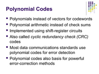
Polynomial Codes
Polynomialsinstead of vectors for codewords
Polynomial arithmetic instead of check sums
Implemented using shift-register circuits
Also called cyclic redundancy check (CRC)
codes
Most data communications standards use
polynomial codes for error detection
Polynomial codes also basis for powerful
error-correction methods
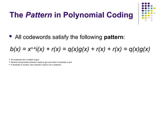
The Pattern inPolynomial Coding
All codewords satisfy the following pattern:
All codewords are a multiple of g(x)!
Receiver should divide received n-tuple by g(x) and check if remainder is zero
If remainder is nonzero, then received n-tuple is not a codeword
b(x) = xn-k
i(x) + r(x) = q(x)g(x) + r(x) + r(x) = q(x)g(x)
138.
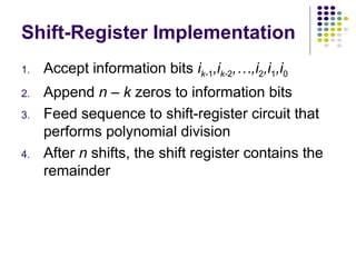
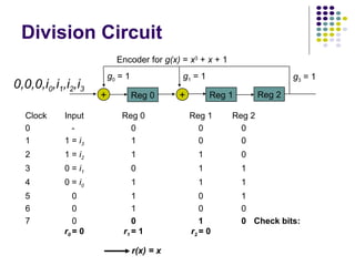
Shift-Register Implementation
1. Acceptinformation bits ik-1,ik-2,…,i2,i1,i0
2. Append n – k zeros to information bits
3. Feed sequence to shift-register circuit that
performs polynomial division
4. After n shifts, the shift register contains the
remainder
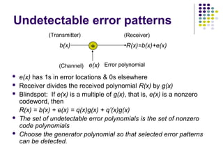
Undetectable error patterns
e(x) has 1s in error locations & 0s elsewhere
Receiver divides the received polynomial R(x) by g(x)
Blindspot: If e(x) is a multiple of g(x), that is, e(x) is a nonzero
codeword, then
R(x) = b(x) + e(x) = q(x)g(x) + q’(x)g(x)
The set of undetectable error polynomials is the set of nonzero
code polynomials
Choose the generator polynomial so that selected error patterns
can be detected.
b(x)
e(x)
R(x)=b(x)+e(x)
+
(Receiver)
(Transmitter)
Error polynomial
(Channel)
141.
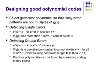
Designing good polynomialcodes
Select generator polynomial so that likely error
patterns are not multiples of g(x)
Detecting Single Errors
e(x) = xi
for error in location i + 1
If g(x) has more than 1 term, it cannot divide xi
Detecting Double Errors
e(x) = xi
+ xj
= xi
(xj-i
+1) where j>i
If g(x) is a primitive polynomial, it cannot divide xm
+1 for all
m<2n-k-1 (Need to keep codeword length less than 2n-k-1)
Primitive polynomials can be found by consulting coding
theory books
142.
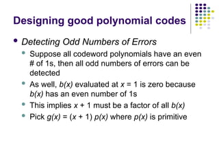
Designing good polynomialcodes
Detecting Odd Numbers of Errors
Suppose all codeword polynomials have an even
# of 1s, then all odd numbers of errors can be
detected
As well, b(x) evaluated at x = 1 is zero because
b(x) has an even number of 1s
This implies x + 1 must be a factor of all b(x)
Pick g(x) = (x + 1) p(x) where p(x) is primitive
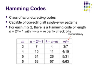
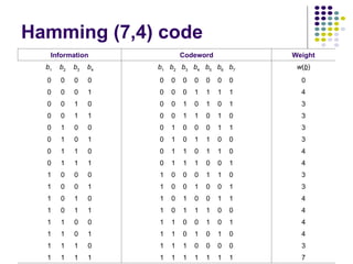
Hamming Codes
Classof error-correcting codes
Capable of correcting all single-error patterns
For each m > 2, there is a Hamming code of length
n = 2m
– 1 with n – k = m parity check bits
m n = 2m
–1 k = n–m m/n
3 7 4 3/7
4 15 11 4/15
5 31 26 5/31
6 63 57 6/63
Redundancy
145.
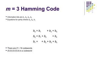
m = 3Hamming Code
Information bits are b1, b2, b3, b4
Equations for parity checks b5, b6, b7
There are 24
= 16 codewords
(0,0,0,0,0,0,0) is a codeword
b5 = b1 + b3 + b4
b6 = b1 + b2 + b4
b7 = + b2 + b3 + b4
Minimum distance ofHamming
Code
Previous slide shows that undetectable error pattern must
have 3 or more bits
At least 3 bits must be changed to convert one codeword
into another codeword
b1 b2
o o
o
o
o
o
o
o
Set of n-
tuples
within
distance 1
of b1
Set of n-
tuples
within
distance 1
of b2
Spheres of distance 1 around each codeword do not
overlap
If a single error occurs, the resulting n-tuple will be in a
unique sphere around the original codeword
Distance 3
150.
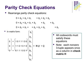
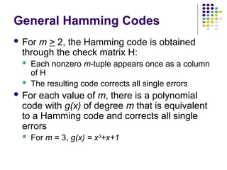
General Hamming Codes
For m > 2, the Hamming code is obtained
through the check matrix H:
Each nonzero m-tuple appears once as a column
of H
The resulting code corrects all single errors
For each value of m, there is a polynomial
code with g(x) of degree m that is equivalent
to a Hamming code and corrects all single
errors
For m = 3, g(x) = x3
+x+1
151.
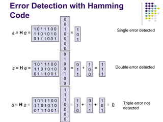
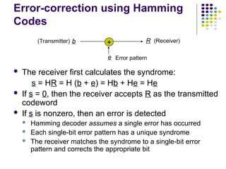
Error-correction using Hamming
Codes
The receiver first calculates the syndrome:
s = HR = H (b + e) = Hb + He = He
If s = 0, then the receiver accepts R as the transmitted
codeword
If s is nonzero, then an error is detected
Hamming decoder assumes a single error has occurred
Each single-bit error pattern has a unique syndrome
The receiver matches the syndrome to a single-bit error
pattern and corrects the appropriate bit
b
e
R
+ (Receiver)
(Transmitter)
Error pattern
152.
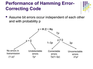
Performance of HammingError-
Correcting Code
Assume bit errors occur independent of each other
and with probability p
s = H R = He
s = 0 s = 0
No errors in
transmission
Undetectable
errors
Correctable
errors
Uncorrectable
errors
(1–p)7
7p3
1–3p 3p
7p
7p(1–3p) 21p2
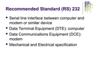
Recommended Standard (RS)232
Serial line interface between computer and
modem or similar device
Data Terminal Equipment (DTE): computer
Data Communications Equipment (DCE):
modem
Mechanical and Electrical specification
155.
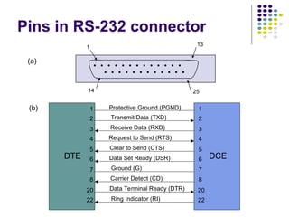
DTE DCE
Protective Ground(PGND)
Transmit Data (TXD)
Receive Data (RXD)
Request to Send (RTS)
Clear to Send (CTS)
Data Set Ready (DSR)
Ground (G)
Carrier Detect (CD)
Data Terminal Ready (DTR)
Ring Indicator (RI)
1
2
3
4
5
6
7
8
20
22
1
2
3
4
5
6
7
8
20
22
(b)
13
(a)
1
25
14
Pins in RS-232 connector
156.
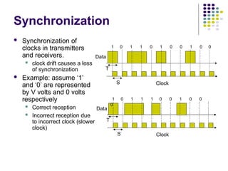
Synchronization
Synchronization of
clocksin transmitters
and receivers.
clock drift causes a loss
of synchronization
Example: assume ‘1’
and ‘0’ are represented
by V volts and 0 volts
respectively
Correct reception
Incorrect reception due
to incorrect clock (slower
clock)
Clock
Data
S
T
1 0 1 1 0 1 0 0 1 0 0
Clock
Data
S’
T
1 0 1 1 1 0 0 1 0 0
0
157.
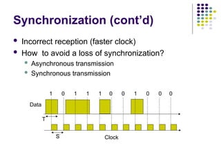
Synchronization (cont’d)
Incorrectreception (faster clock)
How to avoid a loss of synchronization?
Asynchronous transmission
Synchronous transmission
Clock
Data
S’
T
1 0 1 1 1 0 0 1 0 0 0
158.
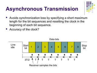
Asynchronous Transmission
Avoidssynchronization loss by specifying a short maximum
length for the bit sequences and resetting the clock in the
beginning of each bit sequence.
Accuracy of the clock?
Start
bit
Stop
bit
1 2 3 4 5 6 7 8
Data bits
Line
idle
3T/2 T T T T T T T
Receiver samples the bits
159.
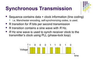
Synchronous Transmission
Voltage
1 00 0 1 1 0 1 0
time
Sequence contains data + clock information (line coding)
i.e. Manchester encoding, self-synchronizing codes, is used.
R transition for R bits per second transmission
R transition contains a sine wave with R Hz.
R Hz sine wave is used to synch receiver clock to the
transmitter’s clock using PLL (phase-lock loop)


![2
2
2
2
1
x
e
x
0
Noise distribution
Noise is characterized by probability density of amplitude samples
Likelihood that certain amplitude occurs
Thermal electronic noise is inevitable (due to vibrations of electrons)
Noise distribution is Gaussian (bell-shaped) as below
t
x
Pr[X(t)>x0 ] = ?
Pr[X(t)>x0 ] =
Area under
graph
x0
x0
= Avg Noise Power](https://image.slidesharecdn.com/3-250809070315-d0d2c8b5/85/3-Digital-transmission-fundamentals-ppt-65-320.jpg)
![1.00E-12
1.00E-11
1.00E-10
1.00E-09
1.00E-08
1.00E-07
1.00E-06
1.00E-05
1.00E-04
1.00E-03
1.00E-02
1.00E-01
1.00E+00
0 2 4 6 8
/2
Probability of Error
Error occurs if noise value exceeds certain magnitude
Prob. of large values drops quickly with Gaussian noise
Target probability of error achieved by designing system so
separation between signal levels is appropriate relative to
average noise power
Pr[X(t)> ]](https://image.slidesharecdn.com/3-250809070315-d0d2c8b5/85/3-Digital-transmission-fundamentals-ppt-66-320.jpg)
![What if bit errors are random?
Many transmission channels introduce bit errors at random,
independently of each other, and with probability p
Some error patterns are more probable than others:
In any worthwhile channel p < 0.5, and so p/(1 – p) < 1
It follows that patterns with 1 error are more likely than patterns with 2 errors and so
forth
What is the probability that an undetectable error pattern occurs?
P[10000000] = p(1 – p)7
and
P[11000000] = p2
(1 – p)6](https://image.slidesharecdn.com/3-250809070315-d0d2c8b5/85/3-Digital-transmission-fundamentals-ppt-123-320.jpg)
![Single parity check code with
random bit errors
Undetectable error pattern if even # of bit errors:
Example: Evaluate above for n = 32, p = 10-3
For this example, roughly 1 in 2000 error patterns is undetectable
P[error detection failure] = P[undetectable error pattern]
= P[error patterns with even number of 1s]
= p2
(1 – p)n-2
+ p4
(1 – p)n-4
+ …
n
2
n
4
P[undetectable error] = (10-3
)2
(1 – 10-3
)30
+ (10-3
)4
(1 – 10-3
)28
≈ 496 (10-6
) + 35960 (10-12
) ≈ 4.96 (10-4
)
32
2
32
4](https://image.slidesharecdn.com/3-250809070315-d0d2c8b5/85/3-Digital-transmission-fundamentals-ppt-124-320.jpg)