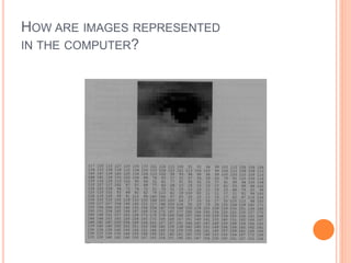
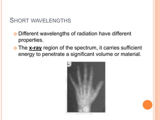
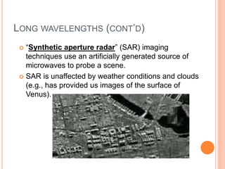
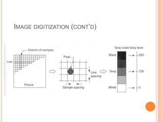
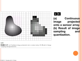
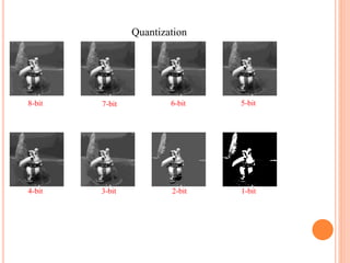
HOW ARE IMAGES REPRESENTED
IN THE COMPUTER?
COLOR IMAGES
A SIMPLE MODEL OF IMAGE FORMATION
 The scene is illuminated by a single source.
 The scene reflects radiation towards the camera.
 The camera senses it via chemicals on film.
PINHOLE CAMERA
 This is the simplest device to form an image of a 3D
scene on a 2D surface.
 Straight rays of light pass through a “pinhole” and
form an inverted image of the object on the image
plane.
CAMERA OPTICS
 In practice, the aperture must be larger to admit more light.
 Lenses are placed to in the aperture to focus the bundle of
rays from each scene point onto the corresponding point in
the image plane
WHAT IS LIGHT?
 The visible portion of the electromagnetic (EM)
spectrum.
 It occurs between wavelengths of approximately
400 and 700 nanometers.
SHORT WAVELENGTHS
 Different wavelengths of radiation have different
properties.
 The x-ray region of the spectrum, it carries sufficient
energy to penetrate a significant volume or material.
LONG WAVELENGTHS
 Copious quantities of infrared (IR) radiation are
emitted from warm objects (e.g., locate people in total
darkness).
LONG WAVELENGTHS (CONT’D)
 “Synthetic aperture radar” (SAR) imaging
techniques use an artificially generated source of
microwaves to probe a scene.
 SAR is unaffected by weather conditions and clouds
(e.g., has provided us images of the surface of
Venus).
CCD (CHARGED-COUPLED DEVICE) CAMERAS
 Tiny solid state cells convert light energy into
electrical charge.
 The image plane acts as a digital memory that can be
read row by row by a computer.
FRAME GRABBER
 Usually, a CCD camera plugs into a computer board
(frame grabber).
 The frame grabber digitizes the signal and stores it in
its memory (frame buffer).
IMAGE DIGITIZATION
 Sampling means measuring the value of an image at a finite
number of points.
 Quantization is the representation of the measured value at the
sampled point by an integer.
IMAGE DIGITIZATION (CONT’D)
IMAGE QUANTIZATION(EXAMPLE)
 256 gray levels (8bits/pixel) 32 gray levels (5 bits/pixel) 16 gray levels (4 bits/pixel)
 8 gray levels (3 bits/pixel) 4 gray levels (2 bits/pixel) 2 gray levels (1 bit/pixel)
IMAGE SAMPLING (EXAMPLE)
original image sampled by a factor of 2
sampled by a factor of 4 sampled by a factor of 8
SAMPLING AND QUANTIZATION
 To convert the image to digital form, we have to
sample the function in both coordinates and in
amplitude. Digitizing the coordinate values is called
sampling. Digitizing the amplitude values is called
quantization.
© 2002 R. C. Gonzalez & R. E. Woods
y (intensity values)
Generating a digital
image. (a) Continuous
image. (b) A scaling
line from A to B in the
continuous image,
used to illustrate the
concepts of sampling
and quantization. (c)
sampling and
quantization. (d) Digital
scan line.
a b
c d
© 2002 R. C. Gonzalez & R. E. Woods
(a) Continuous
image projected
onto a sensor array.
(b) Result of image
sampling and
quantization.
a b
 The one-dimensional function in Fig.2.16(b) is a plot of amplitude
(intensity level) values of the continuous image along the line
segment AB in Fig.2.16(a).
 The random variations are due to image noise.
 To sample this function,we take equally spaced samples along line
AB,as shown in Fig.2.16(c).
 The spatial location of each sample is indicated by a vertical tick
mark in the bottom part of the figure.
 The samples are shown as small white squares superimposed on
the function.
 The set of these discrete locations gives the sampled function.
 However,the values of the samples still span (vertically) a
continuous range of intensity values.
oIn order to form a digital function, the intensity values also must be converted
(quantized) into discrete quantities.
oThe right side of Fig. 2.16(c) shows the intensity scale divided into eight discrete
intervals, ranging from black to white.
oThe vertical tick marks indicate the specific value assigned to each of the eight
intensity intervals.
oThe continuous intensity levels are quantized by assigning one of the eight values
to each sample.
oThe assignment is made depending on the vertical proximity of a sample to a
vertical tick mark.
oThe digital samples resulting from both sampling and quantization are shown in
Fig.2.16(d).
oStarting at the top of the image and carrying out this procedure line by line
produces a two-dimensional digital image.
oIt is implied in Fig.2.16 that,in addition to the number of discrete levels used, the
accuracy achieved in quantization is highly dependent on the noise content of the
sampled signal.
0 0 0 75 75 75 128 128 128 128
0 75 75 75 128 128 128 255 255 255
75 75 75 200 200 200 255 255 255 200
128 128 128 200 200 255 255 200 200 200
128 128 128 255 255 200 200 200 75 75
175 175 175 225 225 225 75 75 75 100
175 175 100 100 100 225 225 75 75 100
75 75 75 35 35 35 0 0 0 35
35 35 35 0 0 0 35 35 35 75
75 75 75 100 100 100 200 200 200 200
Sampling
1024
512
256
128
64
32
Sampling
1024 512 256
128 64 32
imread() – reading an image with different
postfixes
imresize() – resizing an image to any given size
figure – opening a new graphical window
subplot(#of row, # of col, location) – showing
different plots/images in one graphical window
imshow() – displaying an image
im=imread('obelix.jpg');
im=rgb2gray(imread('obelix.jpg'));
im1=imresize(im, [1024 1024]);
im2=imresize(im1, [1024 1024]/2);
im3=imresize(im1, [1024 1024]/4);
im4=imresize(im1, [1024 1024]/8);
im5=imresize(im1, [1024 1024]/16);
im6=imresize(im1, [1024 1024]/32);
figure;imshow(im1)
figure;imshow(im2)
figure;imshow(im3)
figure;imshow(im4)
figure;imshow(im5)
figure;
subplot(2,3,1);imshow(im1);subplot(2,3,2);imshow(im2)
subplot(2,3,3);imshow(im3);subplot(2,3,4);imshow(im4)
subplot(2,3,5);imshow(im5);subplot(2,3,6);imshow(im6)
Quantization
8-bit 7-bit 6-bit 5-bit
4-bit 3-bit 2-bit 1-bit
figure;
subplot(2,4,1);imshow(im1,[]);subplot(2,4,2);imshow(im2,[])
subplot(2,4,3);imshow(im3,[]);subplot(2,4,4);imshow(im4,[])
subplot(2,4,5);imshow(im5,[]);subplot(2,4,6);imshow(im6,[])
subplot(2,4,7);imshow(im7,[]);subplot(2,4,8);imshow(im8,[])

2.ppt

  • 1.
    HOW ARE IMAGESREPRESENTED IN THE COMPUTER?
  • 2.
  • 3.
    A SIMPLE MODELOF IMAGE FORMATION  The scene is illuminated by a single source.  The scene reflects radiation towards the camera.  The camera senses it via chemicals on film.
  • 4.
    PINHOLE CAMERA  Thisis the simplest device to form an image of a 3D scene on a 2D surface.  Straight rays of light pass through a “pinhole” and form an inverted image of the object on the image plane.
  • 5.
    CAMERA OPTICS  Inpractice, the aperture must be larger to admit more light.  Lenses are placed to in the aperture to focus the bundle of rays from each scene point onto the corresponding point in the image plane
  • 6.
    WHAT IS LIGHT? The visible portion of the electromagnetic (EM) spectrum.  It occurs between wavelengths of approximately 400 and 700 nanometers.
  • 7.
    SHORT WAVELENGTHS  Differentwavelengths of radiation have different properties.  The x-ray region of the spectrum, it carries sufficient energy to penetrate a significant volume or material.
  • 8.
    LONG WAVELENGTHS  Copiousquantities of infrared (IR) radiation are emitted from warm objects (e.g., locate people in total darkness).
  • 9.
    LONG WAVELENGTHS (CONT’D) “Synthetic aperture radar” (SAR) imaging techniques use an artificially generated source of microwaves to probe a scene.  SAR is unaffected by weather conditions and clouds (e.g., has provided us images of the surface of Venus).
  • 10.
    CCD (CHARGED-COUPLED DEVICE)CAMERAS  Tiny solid state cells convert light energy into electrical charge.  The image plane acts as a digital memory that can be read row by row by a computer.
  • 11.
    FRAME GRABBER  Usually,a CCD camera plugs into a computer board (frame grabber).  The frame grabber digitizes the signal and stores it in its memory (frame buffer).
  • 12.
    IMAGE DIGITIZATION  Samplingmeans measuring the value of an image at a finite number of points.  Quantization is the representation of the measured value at the sampled point by an integer.
  • 13.
  • 14.
    IMAGE QUANTIZATION(EXAMPLE)  256gray levels (8bits/pixel) 32 gray levels (5 bits/pixel) 16 gray levels (4 bits/pixel)  8 gray levels (3 bits/pixel) 4 gray levels (2 bits/pixel) 2 gray levels (1 bit/pixel)
  • 15.
    IMAGE SAMPLING (EXAMPLE) originalimage sampled by a factor of 2 sampled by a factor of 4 sampled by a factor of 8
  • 16.
    SAMPLING AND QUANTIZATION To convert the image to digital form, we have to sample the function in both coordinates and in amplitude. Digitizing the coordinate values is called sampling. Digitizing the amplitude values is called quantization.
  • 17.
    © 2002 R.C. Gonzalez & R. E. Woods y (intensity values) Generating a digital image. (a) Continuous image. (b) A scaling line from A to B in the continuous image, used to illustrate the concepts of sampling and quantization. (c) sampling and quantization. (d) Digital scan line. a b c d
  • 18.
    © 2002 R.C. Gonzalez & R. E. Woods (a) Continuous image projected onto a sensor array. (b) Result of image sampling and quantization. a b
  • 19.
     The one-dimensionalfunction in Fig.2.16(b) is a plot of amplitude (intensity level) values of the continuous image along the line segment AB in Fig.2.16(a).  The random variations are due to image noise.  To sample this function,we take equally spaced samples along line AB,as shown in Fig.2.16(c).  The spatial location of each sample is indicated by a vertical tick mark in the bottom part of the figure.  The samples are shown as small white squares superimposed on the function.  The set of these discrete locations gives the sampled function.  However,the values of the samples still span (vertically) a continuous range of intensity values.
  • 20.
    oIn order toform a digital function, the intensity values also must be converted (quantized) into discrete quantities. oThe right side of Fig. 2.16(c) shows the intensity scale divided into eight discrete intervals, ranging from black to white. oThe vertical tick marks indicate the specific value assigned to each of the eight intensity intervals. oThe continuous intensity levels are quantized by assigning one of the eight values to each sample. oThe assignment is made depending on the vertical proximity of a sample to a vertical tick mark. oThe digital samples resulting from both sampling and quantization are shown in Fig.2.16(d). oStarting at the top of the image and carrying out this procedure line by line produces a two-dimensional digital image. oIt is implied in Fig.2.16 that,in addition to the number of discrete levels used, the accuracy achieved in quantization is highly dependent on the noise content of the sampled signal.
  • 21.
    0 0 075 75 75 128 128 128 128 0 75 75 75 128 128 128 255 255 255 75 75 75 200 200 200 255 255 255 200 128 128 128 200 200 255 255 200 200 200 128 128 128 255 255 200 200 200 75 75 175 175 175 225 225 225 75 75 75 100 175 175 100 100 100 225 225 75 75 100 75 75 75 35 35 35 0 0 0 35 35 35 35 0 0 0 35 35 35 75 75 75 75 100 100 100 200 200 200 200
  • 22.
  • 23.
  • 24.
    imread() – readingan image with different postfixes imresize() – resizing an image to any given size figure – opening a new graphical window subplot(#of row, # of col, location) – showing different plots/images in one graphical window imshow() – displaying an image
  • 25.
    im=imread('obelix.jpg'); im=rgb2gray(imread('obelix.jpg')); im1=imresize(im, [1024 1024]); im2=imresize(im1,[1024 1024]/2); im3=imresize(im1, [1024 1024]/4); im4=imresize(im1, [1024 1024]/8); im5=imresize(im1, [1024 1024]/16); im6=imresize(im1, [1024 1024]/32); figure;imshow(im1) figure;imshow(im2) figure;imshow(im3) figure;imshow(im4) figure;imshow(im5)
  • 26.
  • 27.
    Quantization 8-bit 7-bit 6-bit5-bit 4-bit 3-bit 2-bit 1-bit
  • 28.