2_Electromagnetic waves and propagation Lectures_part1_1.pdf
1.
LECTURES ON
ELECTROMAGNETIC WAVES
ANDWAVE PROPAGATION
Assoc. Prof. Yasser Mahmoud Madany
Senior Member, IEEE
URSI Senior Member
Founder and Chair of the IEEE Egypt AP-S/MTT-S Joint Chapter
Founder and Counselor of the IEEE AL Ryada Student Branch
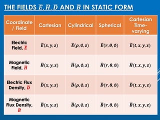
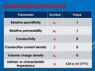
INTRODUCTION
❑ Static electricfield has applications in:
❖ Cathode ray oscilloscopes for deflecting
charged particles.
❖ Ink jet printers to increase the speed of printing
and improve print quality.
❑ Static magnetic field has applications in:
❖ Magnetic separators to separate magnetic
materials from non-magnetic materials.
❖ Cyclotrons for imparting high energy to charged
particles.
4.
INTRODUCTION
❑ Time-varying fieldsconstitute electromagnetic (EM) waves
which have wide applications in all the communications,
radars and also in Bio-medical engineering.
❑ EM waves are produced by time-varying currents.
❑ In brief, it may be noted that:
❖ Static charges produce electrostatic fields.
❖ Steady currents (DC currents) produce magneto-static
fields.
❖ Static magnetic charges (magnetic dipoles) also
produce magneto-static fields.
❖ Time-varying currents produce EM waves or EM fields.
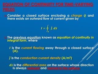
EQUATION OF CONTINUITYFOR TIME-VARYING
FIELDS
❑ Consider a closed surface enclosing a charge 𝑸 and
there exists an outward flow of current given by
𝑰 = ර
𝒔
ҧ
𝑱. 𝒅ത
𝒔
❑ The previous equation known as equation of continuity in
integral form, where
𝑰 is the current flowing away through a closed surface
(A).
ҧ
𝑱 is the conduction current density (A/m2).
𝒅ത
𝒔 is the differential area on the surface whose direction
is always outward and normal to the surface.
7.
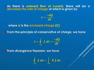
❑ As thereis outward flow of current, there will be a
decrease the rate of charge of which is given by
𝑰 =
−𝒅𝑸
𝒅𝒕
where 𝑸 is the enclosed charge (C).
❑ From the principle of conservative of charge, we have
𝑰 = ර
𝒔
ҧ
𝑱. 𝒅ത
𝒔 =
−𝒅𝑸
𝒅𝒕
❑ From divergence theorem, we have
ර
𝒔
ҧ
𝑱. 𝒅ത
𝒔 = න
𝒗
𝛁. ҧ
𝑱 𝒅𝒗
8.
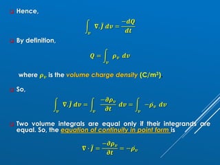
❑ Hence,
න
𝒗
𝛁. ҧ
𝑱𝒅𝒗 =
−𝒅𝑸
𝒅𝒕
❑ By definition,
𝑸 = න
𝒗
𝝆𝒗 𝒅𝒗
where 𝝆𝒗 is the volume charge density (C/m3).
❑ So,
න
𝒗
𝛁. ҧ
𝑱 𝒅𝒗 = න
𝒗
−𝝏𝝆𝒗
𝝏𝒕
𝒅𝒗 = න
𝒗
− ሶ
𝝆𝒗 𝒅𝒗
❑ Two volume integrals are equal only if their integrands are
equal. So, the equation of continuity in point form is
𝛁 ∙ ҧ
𝑱 =
−𝝏𝝆𝒗
𝝏𝒕
= − ሶ
𝝆𝒗
9.
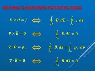
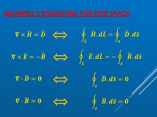
MAXWELL’S EQUATIONS FORTIME-VARYING
FIELDS
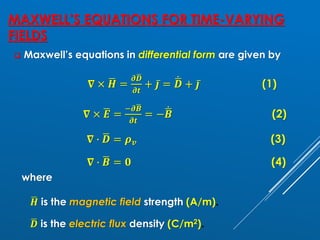
❑ Maxwell’s equations in differential form are given by
𝛁 × ഥ
𝑯 =
𝝏ഥ
𝑫
𝝏𝒕
+ ҧ
𝒋 = ሶ
ഥ
𝑫 + ҧ
𝒋 (1)
𝛁 × ഥ
𝑬 =
−𝝏ഥ
𝑩
𝝏𝒕
= − ሶ
ഥ
𝑩 (2)
𝛁 ∙ ഥ
𝑫 = 𝝆𝒗 (3)
𝛁 ∙ ഥ
𝑩 = 𝟎 (4)
where
ഥ
𝑯 is the magnetic field strength (A/m).
ഥ
𝑫 is the electric flux density (C/m2).
10.
MAXWELL’S EQUATIONS FORTIME-VARYING
FIELDS
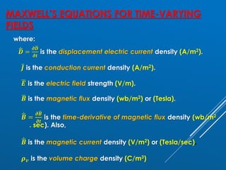
where:
ሶ
ഥ
𝑫 =
𝝏ഥ
𝑫
𝝏𝒕
is the displacement electric current density (A/m2).
ҧ
𝑱 is the conduction current density (A/m2).
ഥ
𝑬 is the electric field strength (V/m).
ഥ
𝑩 is the magnetic flux density (wb/m2) or (Tesla).
ሶ
ഥ
𝑩 =
𝝏ഥ
𝑩
𝝏𝒕
is the time-derivative of magnetic flux density (wb/m2
. sec). Also,
ሶ
ഥ
𝑩 is the magnetic current density (V/m2) or (Tesla/sec).
𝝆𝒗 is the volume charge density (C/m3)
11.
MAXWELL’S EQUATIONS FORTIME-VARYING
FIELDS
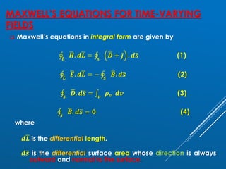
❑ Maxwell’s equations in integral form are given by
ׯ
𝑳
ഥ
𝑯. 𝒅ഥ
𝑳 = ׯ
𝒔
ሶ
ഥ
𝑫 + ҧ
𝒋 . 𝒅ത
𝒔 (1)
ׯ
𝑳
ഥ
𝑬. 𝒅ഥ
𝑳 = − ׯ
𝒔
ሶ
ഥ
𝑩. 𝒅ത
𝒔 (2)
ׯ
𝒔
ഥ
𝑫. 𝒅ത
𝒔 =
𝒗
𝝆𝒗 𝒅𝒗 (3)
ׯ
𝒔
ഥ
𝑩. 𝒅ത
𝒔 = 𝟎 (4)
where
𝒅ഥ
𝑳 is the differential length.
𝒅ത
𝒔 is the differential surface area whose direction is always
outward and normal to the surface.
12.
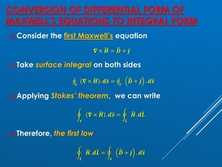
CONVERSION OF DIFFERENTIALFORM OF
MAXWELL’S EQUATIONS TO INTEGRAL FORM
❑ Consider the first Maxwell’s equation
𝛁 × ഥ
𝑯 = ሶ
ഥ
𝑫 + ҧ
𝒋
❑ Take surface integral on both sides
ׯ
𝒔
𝛁 × ഥ
𝑯 . 𝒅ത
𝒔 = ׯ
𝒔
ሶ
ഥ
𝑫 + ҧ
𝒋 . 𝒅ത
𝒔
❑ Applying Stokes’ theorem, we can write
ර
𝒔
𝛁 × ഥ
𝑯 . 𝒅ത
𝒔 = ර
𝑳
ഥ
𝑯. 𝒅ത
𝑳
❑ Therefore, the first low
ර
𝑳
ഥ
𝑯. 𝒅ത
𝑳 = ර
𝒔
ሶ
ഥ
𝑫 + ҧ
𝒋 . 𝒅ത
𝒔
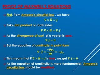
PROOF OF MAXWELL’SEQUATIONS
❑ First, from Ampere’s circuital law , we have
𝛁 × ഥ
𝑯 = ҧ
𝒋
❑ Take dot product on both sides
𝛁. 𝛁 × ഥ
𝑯 = 𝛁. ҧ
𝒋
❑ As the divergence of curl of a vector is zero,
𝛁. ҧ
𝒋 = 𝟎
❑ But the equation of continuity in point form
𝛁 ∙ ҧ
𝑱 =
−𝝏𝝆𝒗
𝝏𝒕
= − ሶ
𝝆𝒗
❑ This means that if 𝛁 × ഥ
𝑯 = ҧ
𝒋 is true, we get 𝛁. ҧ
𝒋 = 𝟎.
❑ As the equation of continuity is more fundamental, Ampere’s
circuital law should be modified.
21.
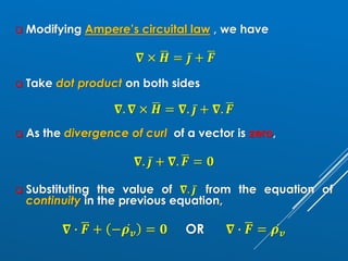
❑ Modifying Ampere’scircuital law , we have
𝛁 × ഥ
𝑯 = ҧ
𝒋 + ഥ
𝑭
❑ Take dot product on both sides
𝛁. 𝛁 × ഥ
𝑯 = 𝛁. ҧ
𝒋 + 𝛁. ഥ
𝑭
❑ As the divergence of curl of a vector is zero,
𝛁. ҧ
𝒋 + 𝛁. ഥ
𝑭 = 𝟎
❑ Substituting the value of 𝛁. ҧ
𝒋 from the equation of
continuity in the previous equation,
𝛁 ∙ ഥ
𝑭 + − ሶ
𝝆𝒗 = 𝟎 OR 𝛁 ∙ ഥ
𝑭 = ሶ
𝝆𝒗
22.
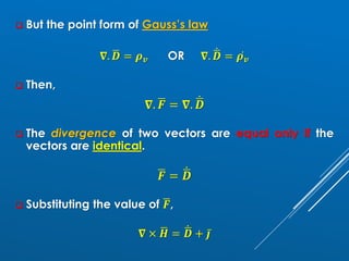
❑ But thepoint form of Gauss’s law
𝛁. ഥ
𝑫 = 𝝆𝒗 OR 𝛁. ሶ
ഥ
𝑫 = ሶ
𝝆𝒗
❑ Then,
𝛁. ഥ
𝑭 = 𝛁. ሶ
ഥ
𝑫
❑ The divergence of two vectors are equal only if the
vectors are identical.
ഥ
𝑭 = ሶ
ഥ
𝑫
❑ Substituting the value of ഥ
𝑭,
𝛁 × ഥ
𝑯 = ሶ
ഥ
𝑫 + ҧ
𝒋
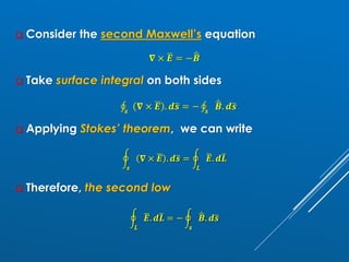
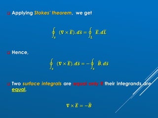
❑ Applying Stokes’theorem, we get
ර
𝒔
𝛁 × ഥ
𝑬 . 𝒅ത
𝒔 = ර
𝑳
ഥ
𝑬. 𝒅ഥ
𝑳
❑ Hence,
ර
𝒔
𝛁 × ഥ
𝑬 . 𝒅ത
𝒔 = − ර
𝒔
ሶ
ഥ
𝑩. 𝒅ത
𝒔
❑ Two surface integrals are equal only if their integrands are
equal,
𝛁 × ഥ
𝑬 = − ሶ
ഥ
𝑩
25.
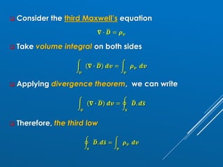
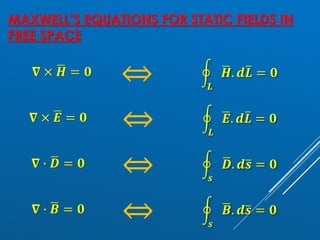
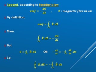
❑ Third, fromGauss’s law in electric field
ׯ
𝒔
ഥ
𝑫. 𝒅ത
𝒔 = 𝑸 = 𝒗
𝝆𝒗 𝒅𝒗
❑ Applying divergence theorem, we get
ර
𝒔
ഥ
𝑫. 𝒅ത
𝒔 = න
𝒗
𝛁 ∙ ഥ
𝑫 𝒅𝒗 = න
𝒗
𝝆𝒗 𝒅𝒗
❑ Two volume integrals are equal only if their integrands are
equal,
𝛁 ∙ ഥ
𝑫 = 𝝆𝒗
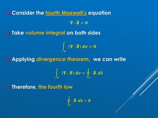
❑ Fourth, from Gauss’s law for magnetic field [the magnetic flux
lines are a closed loop]
ර
𝒔
ഥ
𝑩. 𝒅ത
𝒔 = 𝟎
❑ Applying divergence theorem, we get
𝒗
𝛁 ∙ ഥ
𝑩 𝒅𝒗 = 𝟎 OR 𝛁 ∙ ഥ
𝑩 = 𝟎
26.
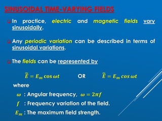
SINUSOIDAL TIME-VARYING FIELDS
❑In practice, electric and magnetic fields vary
sinusoidally.
❑ Any periodic variation can be described in terms of
sinusoidal variations.
❑ The fields can be represented by
෩
ഥ
𝑬 = 𝑬𝒎 𝐜𝐨𝐬 𝝎𝒕 OR ෩
ഥ
𝑬 = 𝑬𝒎 𝒄𝒐𝒔 𝝎𝒕
where
𝝎 : Angular frequency, 𝝎 = 𝟐𝝅𝒇
𝒇 : Frequency variation of the field.
𝑬𝒎 : The maximum field strength.
27.
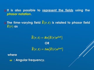
❑ It isalso possible to represent the fields using the
phasor notation.
❑ The time-varying field ෩
ഥ
𝑬(𝒓, 𝒕) is related to phasor field
ഥ
𝑬(𝒓) as
෩
ഥ
𝑬(𝒓, 𝒕) = 𝑹𝒆 ഥ
𝑬 𝒓 𝒆𝒋𝝎𝒕
OR
෩
ഥ
𝑬(𝒓, 𝒕) = 𝑰𝒎 ഥ
𝑬 𝒓 𝒆𝒋𝝎𝒕
where
𝝎 : Angular frequency.
28.
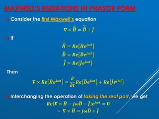
MAXWELL’S EQUATIONS INPHASOR FORM
❑ Consider the first Maxwell’s equation
𝛁 × ෩
ഥ
𝑯 =
෩ሶ
ഥ
𝑫 + ሚҧ
𝒋
❑ If
෩
ഥ
𝑯 = 𝑹𝒆 ഥ
𝑯𝒆𝒋𝝎𝒕
෩
ഥ
𝑫 = 𝑹𝒆 ഥ
𝑫𝒆𝒋𝝎𝒕
෨ҧ
𝑱 = 𝑹𝒆 ҧ
𝑱𝒆𝒋𝝎𝒕
Then
𝛁 × 𝑹𝒆 ഥ
𝑯𝒆𝒋𝝎𝒕
=
𝝏
𝝏𝒕
𝑹𝒆 ഥ
𝑫𝒆𝒋𝝎𝒕
+ 𝑹𝒆 ҧ
𝑱𝒆𝒋𝝎𝒕
❑ Interchanging the operation of taking the real part, we get
𝑹𝒆 𝛁 × ഥ
𝑯 − 𝒋𝝎ഥ
𝑫 − ҧ
𝑱 𝒆𝒋𝝎𝒕 = 𝟎
∴ 𝛁 × ഥ
𝑯 = 𝒋𝝎ഥ
𝑫 + ҧ
𝑱
29.
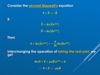
❑ Consider thesecond Maxwell’s equation
𝛁 × ෩
ഥ
𝑬 = −
෩ሶ
ഥ
𝑩
❑ If
෩
ഥ
𝑬 = 𝑹𝒆 ഥ
𝑬𝒆𝒋𝝎𝒕
෩
ഥ
𝑩 = 𝑹𝒆 ഥ
𝑩𝒆𝒋𝝎𝒕
❑ Then
𝛁 × 𝑹𝒆 ഥ
𝑬𝒆𝒋𝝎𝒕 = −
𝝏
𝝏𝒕
𝑹𝒆 ഥ
𝑩𝒆𝒋𝝎𝒕
❑ Interchanging the operation of taking the real part, we
get
𝑹𝒆 𝛁 × ഥ
𝑬 + 𝒋𝝎ഥ
𝑩 𝒆𝒋𝝎𝒕 = 𝟎
∴ 𝛁 × ഥ
𝑬 = −𝒋𝝎ഥ
𝑩
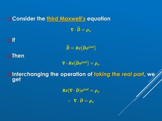
30.
❑ Consider thethird Maxwell’s equation
𝛁 ∙ ෩
ഥ
𝑫 = 𝝆𝒗
❑ If
෩
ഥ
𝑫 = 𝑹𝒆 ഥ
𝑫𝒆𝒋𝝎𝒕
❑ Then
𝛁 ∙ 𝑹𝒆 ഥ
𝑫𝒆𝒋𝝎𝒕 = 𝝆𝒗
❑ Interchanging the operation of taking the real part, we
get
𝑹𝒆 𝛁 ∙ ഥ
𝑫 𝒆𝒋𝝎𝒕 = 𝝆𝒗
∴ 𝛁 ∙ ഥ
𝑫 = 𝝆𝒗
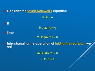
31.
❑ Consider thefourth Maxwell’s equation
𝛁 ∙ ෩
ഥ
𝑩 = 𝟎
❑ If
෩
ഥ
𝑩 = 𝑹𝒆 ഥ
𝑩𝒆𝒋𝝎𝒕
❑ Then
𝛁 ∙ 𝑹𝒆 ഥ
𝑩𝒆𝒋𝝎𝒕 = 𝟎
❑ Interchanging the operation of taking the real part, we
get
𝑹𝒆 𝛁 ∙ ഥ
𝑩 𝒆𝒋𝝎𝒕 = 𝟎
∴ 𝛁 ∙ ഥ
𝑩 = 𝟎
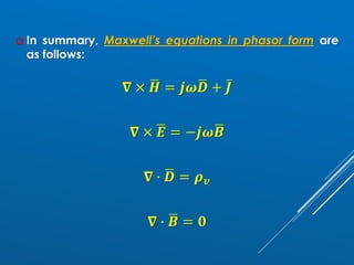
32.
❑ In summary,Maxwell’s equations in phasor form are
as follows:
𝛁 × ഥ
𝑯 = 𝒋𝝎ഥ
𝑫 + ҧ
𝑱
𝛁 × ഥ
𝑬 = −𝒋𝝎ഥ
𝑩
𝛁 ∙ ഥ
𝑫 = 𝝆𝒗
𝛁 ∙ ഥ
𝑩 = 𝟎

![❑ Third, from Gauss’s law in electric field
ׯ
𝒔
ഥ
𝑫. 𝒅ത
𝒔 = 𝑸 = 𝒗
𝝆𝒗 𝒅𝒗
❑ Applying divergence theorem, we get
ර
𝒔
ഥ
𝑫. 𝒅ത
𝒔 = න
𝒗
𝛁 ∙ ഥ
𝑫 𝒅𝒗 = න
𝒗
𝝆𝒗 𝒅𝒗
❑ Two volume integrals are equal only if their integrands are
equal,
𝛁 ∙ ഥ
𝑫 = 𝝆𝒗
❑ Fourth, from Gauss’s law for magnetic field [the magnetic flux
lines are a closed loop]
ර
𝒔
ഥ
𝑩. 𝒅ത
𝒔 = 𝟎
❑ Applying divergence theorem, we get
𝒗
𝛁 ∙ ഥ
𝑩 𝒅𝒗 = 𝟎 OR 𝛁 ∙ ഥ
𝑩 = 𝟎](https://image.slidesharecdn.com/2electromagneticwavesandpropagationlecturespart11-251014090444-844389de/85/2_Electromagnetic-waves-and-propagation-Lectures_part1_1-pdf-25-320.jpg)