neurodegenerative diseases [4].It is observed that the symptoms of AD
slowly worsen over time, damaging the patient’s capacity to perform
routine duties. The experts believe that the basis of this neurological
illness is a mix of genetics, long-term environmental situations, and
lifestyle choices. There is currently no treatment for AD, and all avail
able cures aim to reduce its progression. The treatment puts a long-term
financial strain on individuals, their families, and the government
health-care system [5]. Therefore, building a reliable and efficient
approach for early AD detection is essential. Patients will be able to
make treatment urgently to decrease the progression of the disease.
However, identifying AD in its early stages remains a challenging task.
Because current diagnostic methods depend on clinical judgments,
which are subjective, ignore small indications, and overlap with other
diseases [6]. AD causes dementia, which produces tissue loss throughout
the brain regions and reduces the patient’s cognitive abilities [7].
Therefore, Mild cognitive impairment (MCI) is believed to be a transi
tional stage between age-associated cognitive disease and AD. The MCI
patients are at higher risk of getting AD [8]. The disease stages are
categorized into cognitive normal (CN), MCI, and AD [9].
Brain scanning methods utilize MRI to acquire tomographic images
for the identification of anatomical and functional problems in the brain,
including dementia. MRI scans present images of the brain’s tissues and
other structures using radio waves and a magnetic field. It shows the
structural variations in the brain created due to AD, MCI, and CN dis
orders. It illustrates the changes in the cerebral cortex of Alzheimer’s
patients as the disease develops [10]. It is applied to expose structural
differences between AD patients and healthy persons, as well as to es
timate different phases of AD, such as the expansion of MCI [11].
Diagnosing and treating patients is hard for physicians due to the brain
image’s large volume and complexity. The diagnosis is also
time-consuming and error-prone because such diagnoses depend on the
physician’s knowledge and experience [12]. Brain tumor categorization
is critical for medical evaluation in computer-aided diagnostics (CAD)
[13]. It offers an auxiliary medical image analysis and interpretation
method, enhancing diagnostic precision and reducing radiologists’
burden while producing repeatable results. The combined attempts of
CAD tools and physicians significantly enhance the diagnostic capabil
ities [14]. In past studies, various machine learning (ML) approaches
have been employed to discover the changes in brain MRI images.
However, the images are very complex and have large dimensions, while
these approaches mainly rely on human-designed features, which
frequently lack the depth information required [15]. Additionally, these
approaches require preprocessing like dimensionality reduction, which
results in the loss of important information [16].
The DL models detect the hidden representations and relationship
between distinct parts of the scanned images, and their operation in
identifying AD patterns is often better than that of classic ML approaches
[12]. Convolutional Neural Networks (CNNs) are useful in recognizing
AD-related patterns and abnormalities in brain MRI images. By
inspecting the anatomical and functional variations in the brain, these
algorithms distinguish AD from other types of dementia [17]. However,
the conventional 2D CNN-based approaches fail to effectively extract
diverse brain structures for AD prediction [18]. Some studies have
attempted to deploy 2D CNNs to recognize AD using the input of 2D
slices from 3D MRI images. However, the lack of 3D knowledge de
creases the performance. Despite various research attempts, correct AD
diagnosis and progression estimation remain a difficult task [19]. So,
advanced AD detection and prediction algorithms are needed to assist
medical experts in making an earlier and more accurate diagnosis. The
proposed work develops a novel 3D-CNN model for early AD prediction
to fill these gaps. This work also offers an innovative preprocessing
pipeline encompassing frame selection for dimension reduction, skull
stripping, registration, and noise filtration, tailored to the specific
challenges of neuroimaging data. In architecture level contribution; this
work applies 3D dilated convolution which expands the receptive field
to acquire long-range dependencies across 3D volumetric images. By
fluctuating the dilation rate across layers, the model learns fine-grained
local and global features. This is accomplished without raising the kernel
size or the number of learnable parameters, resulting in improved
computing efficiency. The 3D-CNN model is trained and validated uti
lizing MRI data. The proposed model offers higher diagnostic accuracy
by discovering the brain images’ damaged areas and structural varia
tions. The results illustrate that the proposed 3D-CNN model out
performs earlier models in understanding the brain images while
achieving high accuracy in identifying AD at early stages.
2. Literature review
Early detection of AD has been researched for a long time with the
help of classical image-processing approaches [20,21] along with ML
methods [22]. These methods use handcrafted characteristics to
enhance the model’s capacity to comprehend more complex aspects of
the illness. Classical approaches are focused on the protein side detec
tion of the disease, which is limited to the detection of AD with high
confidence [21]. Nowadays, telehealth systems are growing, assisting
consumers with remote services [23]. Traditional ML algorithms rely on
information collected from the data rather than applying it to the raw
data, which necessitates a lot of work and extensive domain knowledge
[24]. The selection of features significantly impacts the classification
framework’s accuracy, sensitivity, and specificity, among other aspects.
Moreover, the number of parameters in ML methods is much higher, and
single-subject neuroimaging data has millions of dimensions. On the
other hand, DL methods use enhanced feature representation and
extraction approaches to detect AD with high possible confidence and
probability [25]. The DL-based approaches extract features directly
from the input data. The handcrafted feature selection in ML is over
come by automated and self-learning-based feature selection with DL.
DL methods have multiple layers that can automate the feature extrac
tion process by learning to turn the raw data into a more composite
representation at each layer in a subsequent fashion [26]. Some scholars
trained several 3D-CNN architectures using magnetic resonance imaging
(MRI) neuroimaging data and positron emission tomography (PET) for
the multiclass classification of AD. This concentrates on the interaction
between batch normalization and dropout. Three situations were
examined, with the construction trained under scenario 2 (single
dropout layer before the Softmax) attaining the best presentation. In
contrast, scenario 3 (dropout between batch normalization and convo
lution) achieved the worst. Consequences specify that low or no dropout
improves the presentation, while unnecessary dropout harms it, paving
the method for future investigation using integrated MRI-PET datasets
and frequency domain analysis [27]. The study performed in [28]
highlights the formation of lightweight neural networks for
well-organized calculations to identify different stages of AD. The
MobileNet model, primarily designed for mobile applications and rarely
utilized in medical image analysis, was implemented for disease detec
tion. This approach demonstrated superior performance to existing
models, showcasing its potential for accurate and resource-efficient
medical imaging applications. As observed in the literature, DL ap
proaches, such as CNNs [29], recurrent neural networks (RNNs) [30],
SAE [31], and DBNs [32] more effectively extract various characteristics
from MRI images. These methodologies involve converting low-level
features in the data into an abstract high-level representation within
the learning systems [31]. An approach based on the dual-tree complex
wavelet transform extracts features from the input data. Subsequently,
these extracted features are used for classification with a Multi-Layer
Perceptron (MLP) [33]. The CNN comprises convolutional layers,
enabling the model to generate parameters learned from the earlier
layers and facilitating the detection of patterns within the data. CNNs
have demonstrated exceptional accuracy in the classification of features
[34–36]. Two types of CNN architectures for AD classification, including
2D and 3D-CNNs. Some studies have also focused on transfer
learning-based pre-trained models to detect the disease including VGG
A.U. Rahman et al. SLAS Technology 32 (2025) 100265
2
3.
architectures [37]. Theauthors employed the VGG-16 architecture to
accurately classify brain MRI frames into three categories: CN, MCI, and
AD, with the classification performed in binary form. The maximum
accuracy reported is for AD vs CN, which is 98 %. Similarly, AlexNet is
used with transfer learning to detect the disease from healthy subjects
with an accuracy of 95 % [38]. These models are limited to the
pre-trained shapes and sizes of the used models, while the size and
structure of neuroimaging data can be changed from person to person.
Most available CNN architectures are designed for 2D data. In seg
mentation applications aimed at discrimination tasks, CNNs have
consistently demonstrated superior performance to other methodologies
like SVM and logistic regression. CNNs are especially advantageous in
these scenarios due to their strong inherent feature extraction capabil
ities [39]. Computer-based diagnosis (CBD) models built upon CNNs
have exhibited notable success in the detection of neurodegenerative
diseases [40]. 2D-CNNs, including GoogleNet and ResNet, have suc
ceeded in strongly discriminating the healthy from MCI and AD [34].
Using ADNI neuroimaging data, resNet-152 obtained highly discrimi
native features to detect stage (AD, MCI, and CN) progression. Another
deep network called LeNet-5, a CNN architecture proposed by [29],
discriminates AD from the NC brain. In another study, transfer learning
was employed, and the pre-trained VGG-16 was utilized for multiple
classifications of MCI, AD, and CN subjects. This approach leverages the
knowledge acquired by the VGG-16 model on a different task or dataset
and applies it to classifying individuals into three distinct cognitive
states. Transfer learning is a valuable technique in ML and DL, as it can
lead to improved performance by transferring features learned from one
domain to another [41]. Similarly, 3D-ResNet-18 is implemented with
data augmentation to classify different AD stages accurately. ResNet-18
architecture is changed for the two-way classification [42]. The SegNet
is proposed for extracting brain morphological local features to classify
the AD stages [43]. Resnet-101 executed AD, MCI, and CN classification.
All the above studies have focused on the 2D architectures of CNN
models. Leveraging the ADNI dataset, a study employed a fusion
approach based on probability-based CNNs and utilized the DenseNet
architecture [44]. The main goal of this study was to identify AD phases
by functional abnormalities found in the data from neuroimaging. The
main drawback of the 2D CNNs is they cannot detect the flow of struc
tural changes in neuroimaging data. The proposed work focuses on
developing a 3D-CNN architecture for MRI image processing. This
3D-CNN is designed to create a classifier capable of distinguishing be
tween CN, MCI, and AD based on brain MRI images. In this context,
3D-CNNs capture three-dimensional spatial information from the MRI
data, making them particularly suitable for tasks involving volumetric
image data like brain scans. Using MRI images, the objective is to
employ this specialized architecture to accurately classify the cognitive
states, CN, MCI, and AD. The latest advancements in DL have driven
important growth in neuroimaging-based AD forecasting. Numerous
works have discovered 2D and 3D approaches to perform such type of
tasks. However, the proposed study, deployed a novel approach of
preprocessing, intelligent frame selection, and modification in the ar
chitecture of 3D-CNN (3D dilated convolution), which make this study
unique for AD prediction.
2.1. Previous works limitations
It is observed from the literature that many researchers have focused
on using 2D-CNN for AD prediction. However, MRI scans contain 3D
volumetric data, where each slice is processed separately by 2D CNNs.
This method eliminates certain depth information and spatial context
between adjacent slices. The lack of extracting complete anatomical
features makes detecting disorders that depend on 3D structural context
harder. Additionally, it fails to recognize the relationships between sli
ces, which are crucial for detecting abnormalities. Some studies use
transfer learning for 2D-CNN architectures to enhance the prediction
performance and avoid the respective model’s overfitting. Transfer
learning is limited by unchangeable dimensions of the input data and
hidden layers, which might not suit all the cases. Similarly, 2D-CNN
architectures cannot detect the temporal changes in the structures of
the neuroimaging data.
2.2. Key contributions
In this research, along with a standard preprocessing pipeline, an
efficient frame selection and cropping-based dimensions reduction
method is proposed for the stage detection of AD. The reduced input
dimensions have the benefit of avoiding the model’s overfitting and
underfitting problems. Moreover, unlike prior studies that often focused
on 2D-CNNs or transfer learning, a sparse 3D architecture is proposed in
this study, rather than using predefined CNN deep models to enhance
the detection results of all the three stages of the disease, i.e., CN, MC,
and AD. The following are the contributions of the proposed work.
• Intelligent Preprocessing Pipeline: This study offers an innovative
preprocessing pipeline encompassing frame selection for dimension
reduction, skull stripping, registration, and noise filtration, tailored
to the specific challenges of neuroimaging data.
• Integration of 3D-CNNs: This work introduces a novel 3D-CNNs ar
chitecture, enabling the comprehensive analysis of both spatial and
temporal structural changes in AD from MRI data.
• 3D dilated Convolution: This work employs 3D dilated convolution,
which expands the receptive field, allowing the model to capture
long-range dependencies across 3D MRI images.
• Improved Prediction Performance: The proposed approach enhances
prediction accuracy by combining 3D-CNNs with efficient data pre
processing achieving an average accuracy of 92.89 %.
3. Proposed methodology
Fig. 1 shows the steps conducted to complete the proposed meth
odology. The raw MRI data is preprocessed initially to remove noisy
data. The number of frames in all three MRI views is very high
(150–200), but here the most informative frames are selected. Finally,
3D-CNN architectures are applied. The overall process is conducted,
such as the 3D MRI scans, which have uniform dimensions, which are
given as input to the model. After that, several 3D convolution layers,
followed by batch normalization, ReLU activation, and max-pooling, are
applied. In this work, we used different filters (32, 64, 128) to get
optimal performance. The output of the convolution layer is then passed
to the flattening layer. The output from the flattened layer is then passed
to the fully connected layer. The final layer with the softmax activation
function is used to get the final output of the model.
3.1. Dataset
The MRI data used in this study were initially produced and provided
by the Alzheimer’s Disease Neuroimaging Initiative (ADNI) [39,40],
including AD, CN, and MCI classes. The collection comprises 3D MRI
scans from 221 different people, stored as DICOM files. This dataset
provides multiple visits for the same patient, amounting to nearly 7000
NIFTI files, each containing 3D-view MRI images. For this study,
T1-weighted data spanning three years was considered, resulting in a
subset of 2182 NIFTI files. Each NIFTI file comprises an individual
subject’s sagittal, coronal, and transverse views, totaling over 250
sequential frames across all three views. This dataset comprises 748 CN,
981 MCI, and 453 CE samples. The dataset is also balanced regarding
gender representation, with 1279 male and 930 female subjects. Addi
tionally, the average age of the subjects is 76.23 years, with a standard
deviation of 6.8 years, showing a broader range. Furthermore, each
subject in the dataset contributed an average of 4.1 visits, providing a
rich longitudinal perspective on cognitive health changes. This
comprehensive dataset is valuable for research, offering insights into the
A.U. Rahman et al. SLAS Technology 32 (2025) 100265
3
4.
relationship between age,gender, and cognitive health.
3.2. Preprocessing
Preprocessing is one of the key steps in medical imaging. We
employed first the basic preprocessing approaches, like intensity
normalization, noise reduction, and data augmentation. These steps
confirm that the input MRI data is now reliable for the 3D-CNN model
for feature extraction. Table 1 highlights the important preprocessing
approaches, their unique elements, and precise instances for AD pre
diction. The standard preprocessing medical imaging pipeline used in
this work includes the following steps:
Skull stripping: This step involves the process of eliminating non-
brain tissues, such as the skull and scalp, from MRI images to empha
size exploration only of brain constructions. In this work, we employed
SimpleITK to remove non-brain tissues
Spatial normalization: This step is performed for aligning and
converting brain images to a standard anatomical space to permit reli
able comparison across diverse issues. We employed Nilearn for spatial
normalization.
Smoothing: It is a preprocessing method in neuroimaging that
moderates clamor and improves signal recognition by employing a
Gaussian filter to the image data.
Slicing and resizing: It includes extracting particular cross-sectional
slices from 3D neuroimaging data and changing their dimensions to
certify identical input sizes for examination or model training.
These preprocessing methods differ from conventional approaches
by integrating advanced machine learning procedures, advanced spatial
normalization with adaptive Gaussian smoothing, anatomical priors,
and content-based resizing. Contrasting traditional methods that rely on
basic thresholding, fixed cropping, or uniform smoothing the proposed
approaches certify larger precision, better alignment, and more reliable
data, which increases the whole performance of the 3D-CNN model.
Frame Selection and Cropping: Effective processing of 3D MRI
data needs to decrease the computational load without dropping the
diagnostic performance of the model. To perform this, the proposed
technique includes an intelligent frame selection and cropping strategy,
ensuring that only the most applicable portions of the MRI data are
extracted.
Frame Selection: We implemented a frame selection mechanism
instead of processing the whole 3D MRI images, which is computa
tionally costly and does not provide redundant data. This method rec
ognizes slices from the MRI volume that are most likely to contain
diagnostically important features for AD prediction. The collection is
directed by statistical and anatomical principles:
• Statistical Criteria: Frames are graded based on strength circula
tions and voxel variance, certifying that specific slices involve
important data rather than identical or noisy areas.
• Anatomical Criteria: Frames matching to main brain sections
related to Alzheimer’s ailment pathology, such as the medial tem
poral lobe and hippocampus are selected.
This selection decreases the amount of frames processed while
maintaining acute investigative information, assisting the model to
emphasize applicable features and patterns.
Fig. 1. The steps conducted to complete the proposed methodology.
Table 1
Preprocessing steps for Alzheimer’s disease prediction.
Preprocessing
Technique
Description Novel Approach Example
Skull Stripping Removes non-brain tissues (e.g., skull, scalp) Utilizes segmentation Applying a segmentation tool to automatically
extract brain regions
Spatial
Normalization
Aligns MRI scans to a standard anatomical
template (e.g., MNI152)
Incorporates anatomical priors and refined
warping techniques
Normalizing brain scans to the MNI152 template
Smoothing Reduces high-frequency noise and smooths out
variations in the scan
Gaussian smoothing with adjustable
parameters
Applying a 6 mm FWHM Gaussian filter
Slicing and Resizing Slices MRI scans into smaller sections Adapts slicing and resizing based on content Resizing each MRI slice
A.U. Rahman et al. SLAS Technology 32 (2025) 100265
4
5.
Frame Cropping: Thecropping step is employed to separate the
region of interest (ROI) within each frame after selecting the diagnos
tically applicable frames. This step has the subsequent elements:
• ROI Detection: Bounding boxes are produced near the brain area
using a segmentation procedure to eliminate inappropriate parts,
such as surrounding non-brain tissues and background.
• Standardized Cropping: Every nominated frame is cropped to a
fixed size (e.g., 128×128 pixels), ensuring consistency across the
dataset and decreasing computational overhead.
The cropping process improves the emphasis of the 3D-CNN model
on disease-specific features, refining its capacity to distinguish certain
patterns related to Alzheimer’s ailment.
Impact of Frame Selection and Cropping: The frame selection and
cropping procedures contribute to the model’s competency and
accuracy:
• Efficiency Gains: The computational time of training and testing is
considerably reduced by decreasing the number of frames and
concentrating on ROIs. This allows the usage of DL models with
larger datasets while utilizing limited resources.
• Improved Accuracy: Eliminating unrelated data ensures that the
model is exposed to learn only critical patterns more relevant to the
disease pattern, which improves the diagnostic accuracy of the
model.
The MRI data based on T1-Weighted in NIFTI format from the dataset
is preprocessed with the help of the CAT12 toolkit. This tool is provided
by the SPM12, which is a third-party MATLAB toolbox. The MRI images
were transformed to adhere to the dimensions of 121×145×121 (X × Y
× Z) with a spatial resolution of 1.5 × 1.5 × 1.5 mm3 per voxel.
Furthermore, all MRI images underwent signal intensity normalization,
where each voxel value was normalized by dividing it by the maximum
value of the MRI. The 3D-MRI data consisting of 121×145×121 di
mensions for transverse, sagittal, and coronal views were acquired
through re-slicing, resulting in dimensions of (145×121), (121×121),
and (121×145), respectively. Subsequently, edge padding and zero
filling were applied, and all 2D frames were resized to dimensions of
(145×145). The process of skull stripping involves the removal of non-
cerebral tissues such as the skull, scalp, and dura from brain images. One
method used for this purpose is Adaptive Probability Region-Growing
(APRG), which refines probability through region-growing methods
[45]. Currently, the APRG method is the most accurate and dependable
approach for skull removal in brain MRI data. In our research, we have
successfully employed the APRG method to eliminate the skull from the
MRI data.
The brains of humans exhibit variations in shapes among individuals.
One primary objective of spatial normalization is to deform the scans of
the brain in a way that aligns with a specific location. It involves
transforming images from different subjects into a common coordinate
system, ensuring that anatomically corresponding regions are in uni
form positions. Spatial normalization can be considered a specialized
form of image registration. Its purpose is to map an MRI image of an
individual onto the brain’s reference space, enabling comparisons be
tween subjects with diverse brain morphologies. In this work, DARTEL
registrations were utilized to achieve spatial registration. This involved
aligning the individual MRI images with an existing template, facili
tating the comparison of brain scans across subjects with varying brain
structures [46]. Smoothing is a technique for eliminating various types
of noise present in MRI frames. This study employed a Gaussian filter to
reduce noise in the MRI data.
A substantial number of frames per view, totaling nearly 150 frames
for each set of MRI images following preprocessing. This enormous
number of frames requires incredible processing resources to train a
CNN model. Furthermore, overfitting of the CNN may result from data
redundancy. Recently, various studies have used a random selection
technique to overcome this difficulty. More precisely, the study in [36]
used 33 transverse frames, 40 sagittal frames, and 50 coronal frames,
which were randomly selected, yielding 123 frames taken from a sub
ject’s 3D brain imagery. This decrease in the total number of frames
assists in reducing the computing requirements and any overfitting
difficulties that come with training a CNN model on such big datasets.
The proposed framework deployed an innovative frame selection
method. This approach recognizes and ranks parts that show robust
associations with Alzheimer’s pathology, efficiently decreasing noise
and computational time while conserving critical diagnostic facts.
However, it is hard to discover which frame has the most valuable in
formation, so randomly picking frames might not be compelling. This
random selection method might result in the loss of critical data. In our
research, we adopted a different strategy by choosing frames based on
statistical analysis. To begin, we calculated the number of informative
pixels using Eq (1). Frames with fewer informative pixels than the
threshold value were discarded.
I = 1 −
N0
HI × WI
(1)
The total number of zeros is represented by N0 in an image with the
height of HI the width of WI. In this study, the top 40 informative frames
from each view are chosen, leading to a total of 120 frames per patient in
the analysis. The frames that were selected based on statistical criteria
effectively lowered the computational complexity of MRI processing.
Each frame encompassed varying sizes of informative regions. To
establish an average window size for all patients across the three views,
we employed the proposed algorithm, referred to as Algorithm 1. The
computational complexity of the proposed model expressively reduced
after frame selection, with reductions of nearly 92 % in input data size,
87 % training time decrease, and 90 % lessening in inference time,
together with a 75 % reduction in GPU memory utilization. This high
lights the productivity of smart frame selection in enhancing resource
usage while stabilizing model presentation. Table 2 represents the
computational complexity comparison before and after frame selection
of the proposed model.
3.3. Model development
The proposed model is employed to capture the spatial and volu
metric features of MRI data widely. It includes improved layers for
deeper feature extraction and leverages a tailored learning rate opti
mization method for effectual training. Fig. 2 represents the architecture
of the proposed 3D-CNN model used in this study.
The proposed work has applied 3D architecture, in which a shallow
3D-CNN architecture, i.e., width × height × view × number_of_frames, is
proposed and compared with recent research that has used 3D-CNN for
the classification of AD [36]. The proposed 3D-CNN is used to capture
the information from all three views at the same time. In this study, a
shallow 3D-CNN architecture that is especially targeted towards classi
fying AD is proposed. This architecture is made to analyze
multi-dimensional data. By concurrently weighing data from several
points of view or vantage points, it aims to advance earlier studies and
produce more reliable and accurate results for the diagnosis of AD.
Input Layer: The MRI images are 3D volumetric data denoted as a
tensor X having a shape (D, H, W, C). Where D represents depth (number
of slices), H height of each slice, W width of the slice, and C number of
channels.
3D Convolution Layer: The convolution layer employs a 3D kernel
across the input data to create feature maps that maintain depth. The 3D
kernel K with shape (kd,kh,kw,C), the convolution operation is described
in Eq (2).
A.U. Rahman et al. SLAS Technology 32 (2025) 100265
5
6.
Yi,j,k =
∑
C
c=1
∑
kd− 1
p=0
∑
kh−1
q=0
∑
kw− 1
r=0
Xi+p,j+q,k+r,c⋅Kp,q,r,c + b (2)
Where Y shows the output feature map, (i, j, k) shows the position of
the feature map, and b is the bias term.
Activation Function: For introducing non-linearity to learn com
plex patterns in the MRI data, Rectified Linear Unit (ReLU) is applied. It
is defined as shown in Eq (3).
Y
ʹ
i,j,k = max
(
0, Yi,j,k
)
(3)
Where, Yi,j,k the represented the input to the activation function and
Y
ʹ
i,j,k indicate outputs as the input value, if it is positive otherwise 0 if the
input is negative, presenting non-linearity to the model.
3D Max Pooling: For preserving only the prominent features, max
pooling is used. It downsamples the feature maps by choosing only the
maximum value in the specific window. For the input Yʹ using a pooling
window P of size (pd,ph,pw), the pooling operation is described in Eq. (4).
Zi,j,k = max
0≤m<pd,0≤n<ph,0<o<pw
Yʹ
ipd+m,j.ph+n,k.pw+o
(4)
It mines the extreme value from a distinct 3D area of the input Yʹ,
decreasing its dimensions while recalling the most important features.
Fully Connected Layers: Using several convolutional and pooling
layers, the 3D feature is flattened into a 1D vector and passed to the fully
connected layers. It combines the high-level features from the entire
MRI image to perform the final predictions as discussed in Eq (5).
z(l+1)
= f
(
W(l)
z(l)
+ b(l)
)
(5)
Where z represents the flattened vector, the W(l)
represents weights
and biases of layer l is denoted by b(l)
, the input to the layer z(l)
. The
activation function is represented by f employed to z(l+1)
find the output
for the resulting layer.
Output Layer: For three class classifications, the softmax activation
function is used. It outputs the probability scores for each class as rep
resented in Eq (6).
Softmax(z) =
exp(zi)
∑
jexp
(
zj
) (6)
The input to the softmax function is a vector represented by (z) = [z1,
z2, …, zn], where each zi signifies the score for the ith
class in a classifi
cation tricky. The Softmax function used the exponential oper
ationexp(zi) for each sore each zi. The numerator exp(zi) is divided by
the summation of exponentials of all scores
∑
jexp
(
zj
)
.
4. Experiments
In this work, various experiments are conducted to assess the effec
tiveness of the proposed 3D-CNN architecture for the categorization of
AD. This work also focused on the 3D-CNN architectures to avoid the
model’s underfitting and overfitting problems. The architectures of 3D-
CNN are shown in Fig. 2, where C stands for the convolutional layer, P
for the pooling layer, and FC for the fully connected layer. The archi
tecture is shallow because of intelligent frame selection and cropping, as
compared to the literature. [47]. The proposed 3D-CNN model contains
a total number of learnable parameters are 1091,475, which shows its
complexity and volume for classification and feature extraction.
Algorithm 1
Skull stripping, smoothing, and frame selection.
Input: # number of images
Output: preprocessed image
For each image in the image list
Load the image
Skull stripping:
Use skull stripping algorithm to eliminate non-brain tissues
Save the skull-stripped image
Smoothing:
Use a smoothing algorithm to decrease noise
Save the smoothed image
Frame Selection:
Analyze the image content and motion to choose the frame
Save the selected frame
Save the results:
Save the preprocessed images
End loop
Table 2
Complexity comparison before and after frame selection.
Parameter Before After Reduction
(%)
Total frames 150 120 20
Input volume (reduction in
depth)
256×256×150 256×256×120 23
Memory usage (per batch) 629MB 409MB 35
Training time (per epoch) 3 h 2.43 h 19
Inference time (per epoch) 30 s 22.8 s 24
Fig. 2. The architecture of the proposed 3D-CNN model used in this study.
A.U. Rahman et al. SLAS Technology 32 (2025) 100265
6
7.
4.1. 3D dilatedconvolutions
Alzheimer’s disease is characterized by common neurological
changes in several locations. We used the 3D dilated convolutions
approach using MRI images to capture minor and diffuse structural al
terations across the brain. This approach increases the receptive field of
the convolutional kernel without raising the number of parameters. The
standard convolutions examine surrounding voxels within a given
kernel size, but dilated convolutions create "holes" between kernel ele
ments. It effectively improves the depth of the input volume. The depth
is determined by a dilation factor, which controls the distance between
kernel elements. At d = 1, it becomes a conventional convolution. To
optimize efficacy, dilation factors are gradually raised between layers
(for example, d = 1, 2, 4, 8). This enables the model to learn hierarchical
characteristics at deeper levels before progressing to larger regions.
During experimentation, we observed that this strategy is beneficial for
3D MRI imaging. It eliminates the requirement for downsampling layers
(such as pooling), which sometimes lose essential spatial features. The
dilated convolutions allow the model to acquire both local and global
information quickly. It captures multi-scale characteristics of Alz
heimer’s development, such as cortical thinning and hippocampal at
rophy, which improves the model’s accuracy.
4.2. Early stopping
Early stopping is used to avoid overfitting the 3D-CNN model. The
initial learning rate was set to 0.001. Early stopping was monitored
using the validation accuracy during training. Patience to stop the
training processes was set to 4.
4.3. Reduce learning rate
Another useful callback in any deep learning model is to reduce the
learning rate by a certain factor. This callback is useful when the model
cannot find the best global solution and is stuck in the local optimum
solution. Similarly, the accuracy of the validation also monitors the
reduced learning rate. The reduction factor on each step is 0.01, while
the patience was set to 2. The minimum value for the learning rate is
kept at 0.0001.
4.4. Checkpoint
This callback is useful for storing the best weights of the model
during training. Those weights were considered the best, with the
highest validation accuracy while training the CNN model. Table 3
shows detailed parameters of the callbacks used to improve the model’s
performance. Checkpoints save the model’s weights and state during
training, making it useful for lengthy procedures like 3D-CNN training.
To reduce the possibility of overfitting, the model halts training if the
accuracy does not improve after several epochs.
4.5. Environmental setup
The proposed methodology is implemented with MATLAB and Py
thon installed on Windows 10. MATLAB was used to preprocess the MRI
data, while Python was used for feature selection, model training, and
comparative analysis. The system used for the experimental work was a
core i7 Central Processing Unit (CPU) with a RAM of 16 GB. The libraries
used for this research included Keras/TensorFlow, Scikit-Learn, NiBabel,
and Plotly. The CAT-12 toolbox of SPM12 provided by MATLAB is used
to preprocess the raw MRI files.
4.6. Performance measures
The performance parameters used in this research are reported in
terms of accuracy, precision, recall, and F-measure. The equations for all
four performance measures are given in Eq (7), (8), (9), and (10). True
Positive (TP) are those instances whose ground label is true and is pre
dicted as true as well while True Negative (TN) are false and predicted as
false as well. Moreover, False Positive (FP) is negative but predicted as
positive while False Negative (FN) is positive but predicted as negative.
Precision =
TP
TP + FP
(7)
Recall =
TP
TP + FN
(8)
F1 Score =
2 ∗ (Recall ∗ Precision)
(Recall + Precision)
(9)
Accuracy =
TP + TN
TP + FN + FP + TN
(10)
5. Results and discussion
The proposed 3D-CNN architecture is built to extract features from
the multi-view 3D data effectively. We utilized data augmentation
strategies, such as random rotations, translations, and flips, to avoid
overfitting and enhance the model’s generalization. The number of
epochs required to train and validate the 3D-CNN model is 160. After
160 epochs, the model automatically stopped training as the model was
going to overfit. Training and validation plots for 3D data are depicted in
Fig 3. Similarly, the loss of the model is reflected in Fig 4. Table 4 rep
resents the CM-1 confusion matrix of 3D-CNN. CM-1 shows the confu
sion matrix compiled between the actual labels and predicted labels. The
validation plots of the 3D-CNN are much smoother and diverging while
training. It shows that the 3D-CNN captures the information from all
three views at the same time, which avoids the model’s underfitting. Due
to the high dimensions of input data for 3D-CNN, it also avoided the
model’s overfitting as compared to other CNN models. Table 5 shows the
training and testing accuracy achieved by the proposed model of each
class. The other performance measures, like average precision, recall,
and F1-score reported by the proposed methodology are 91.99 %, 92.54
%, and 92.21 %, respectively as shown in Table 6. A 2D-CNN examines
data in two dimensions using each convolutional layer. However, the
3D-CNN captures the characteristics that evolve or change over the third
dimension as well, which is crucial in jobs like tracking disease pro
gression in medical imaging.
5.1. Comparison with closely related works
From the complete set of experiments performed on 3D-CNN archi
tecture, this research has analyzed the fact that data size can affect the
performance of any DL model. Fig 5 shows the overall performance
between the 3D-CNN architecture proposed by this research and the
state-of-the-art CNN models. Compared to the literature, the proposed
3D-CNN performance is much better, and the model converges properly
Table 3
Configuration parameters used in this study.
Parameter Configuration
Learning rate 0.001
Reduction factor 0.1
Reduction Patience 2 times
Patience to stop 4 times
Stopping criteria Validation accuracy
Initial weights Random
Trainable Yes
Optimizer Adam
Loss Categorical cross-entropy
Epochs 160
Performance Metric Accuracy
Training, testing, validation 70, 15, 15
Batch size 64
A.U. Rahman et al. SLAS Technology 32 (2025) 100265
7
8.
because of thesimultaneous extraction of features from data. The fitting
of CNN models depends on the number of learnable parameters in any
DL model. Table 7 depicts the overall comparison between the proposed
3D-CNN architecture and the most relevant literature. The authors in
[47] used 123 random frames selected from the input preprocessed data,
trained all the 123 2D models separately, and then took the average of
all the accuracies. It is observed that the number of parameters in [47]
has 1.227 M parameters, which is more than the 2D-CNN architecture
proposed by this research. The performance of the proposed model is
8+% greater than the literature [47]. Although the accuracy difference
between the proposed method and the transfer learning-based 2D
VGG-19, [37], is almost 5 %. However, the number of parameters in our
proposed method is 127 times less than their method, which is a great
achievement.
Moreover, the dataset size is almost 7 times less than the proposed
work selected dataset. The number of parameters is much higher than
ours and the dataset size is also very small as compared to the proposed
work. Thus, the experimental results reflect that the intelligent
Fig. 3. Training and testing accuracy of the proposed model.
Fig. 4. Training and testing loss of the proposed model.
Table 4
CM-1 confusion matrix of 3D-CNN.
CN MCI AD
CN 135 7 8
MCI 4 187 5
AD 3 4 83
Table 5
Accuracy achieved by the proposed model.
Class Training Accuracy (%) Testing Accuracy (%)
AD 92.38 90.15
CN 94.62 91.21
MCI 93.75 92.89
Average 93.58 91.41
Table 6
Results obtained using the proposed model.
Class Precision (%) Recall (%) F1-score (%)
AD 86.46 92.22 89.25
CN 95.07 90.00 92.47
MCI 94.44 95.41 94.92
Average 91.99 92.54 92.21
A.U. Rahman et al. SLAS Technology 32 (2025) 100265
8
9.
preprocessing methods andframe selection approach improve the
model’s accuracy. Compared to current state-of-the-art works, the pro
posed 3D-CNN reached the highest accuracy of 92.89 % for AD
prediction.
5.2. Discussion
The 3D-CNN model used in this research has a much smaller number
of learnable parameters as compared to other relevant studies [36].
They performed various experiments and the best classification accuracy
the authors have reported is 84.57 %, which is 8 % less than the pro
posed 3D-CNN architecture used in this study. Moreover, the number of
subjects is just 988, which is quite low compared to our selected dataset.
The possible reason is that the number of parameters in the proposed
3D-CNN is almost 10 times less than the models used in the literature.
Similarly, [44] has used a much larger dataset size but their number of
parameters is greater than our proposed method while the accuracy is
less than ours. The authors have used 3D DenseNet-121 architecture for
training and prediction of the disease. Our proposed model performance
is almost 8 % greater than [44], and the reason is our intelligent frames
selection and cropping, and the simpler CNN architecture we have
proposed in this study. The study also emphasizes how effective model
architecture and data size affect DL models’ overall effectiveness. The
suggested model expands the potential for precise and effective AD
diagnosis and progressing monitoring by attaining competitive precision
outcomes with fewer parameters. (Table 8)
We conducted an ablation study to assess the influence of each factor
in the proposed 3D-CNN model. The study thoroughly examined various
components, like preprocessing steps, the frame selection scheme, and
particular CNN layers, to measure their distinct effect on the model’s
operations. This conveys critical intuitions into the implication of each
element in the proposed model. The complete model, which contains
preprocessing, frame selection, and all CNN layers along with 3D dila
tion, achieves the highest accuracy (92.89 %) and F1 score (92.21 %).
This configuration shows the model’s capacity to balance computational
time and diagnostic performance efficiently. The accuracy and F1-score
drop to 87.2 % and 85.7 %, respectively when preprocessing is omitted,
despite a minor reduction in computational time. This highlights the
significance of preprocessing in improving input data quality and
enabling better feature extraction. Similarly, eliminating frame selection
decreases the model’s accuracy to 89.8 % and F1-score to 87.5 %. This
consequence approves the critical role of preprocessing, and frame se
lection in removing inappropriate frames and concentrating on focused
areas, which decreases noise and enhances model accuracy.
6. Conclusions
This work developed a novel preprocessing, intelligent frame selec
tion, and 3D-CNN based approach for AD prediction. During the
experimentation, we observed that CNNs are highly dependent on the
input data. If the data is clean and informative, and the model will
extract large amounts of information, it will produce better results. This
research has concluded this phenomenon through various experimental
results. We also observed that, training on the less informative data
results in the overfitting of CNN architectures. Similarly, a CNN with
more learnable parameters will take more time to learn, also sometimes
will lead to overfitting and vice versa. In the case of 2D-CNN, it extracts
Fig. 5. Results comparison with closely related works.
Table 7
Results comparison with state-of-the-art works.
Author Architecture Subjects Parameters No of
Models
Accuracy
(%)
[47] 2D-CNN 509 1227,731 123 84.05
[37] 2D VGG-19 300 138,423,208 1 87.15
[36] 3D-CNN 988 10,467,315 1 84.57
[44] 3D DenseNet-
121
3512 7628,484 1 84.00
Proposed 3D-CNN 2186 1091,475 1 92.89
Table 8
Ablation study results of the proposed model.
Configuration Preprocessing Frame
Selection
Accuracy
(%)
F1-Score
(%)
Full Model Yes Yes 92.89 92.21
Without
Preprocessing
No Yes 87.2 85.7
Without Frame
Selection
Yes No 89.8 87.5
Reducing
Convolutional
Layers
Yes Yes 88.1 86.9
A.U. Rahman et al. SLAS Technology 32 (2025) 100265
9
10.
features limited to2D spatial domains, often lacking volumetric patterns
like atrophy in brain regions, which span across 3D spaces. It ignores the
depth, which results in the loss of inter-slice spatial information. We also
observed that the 2D-CNN requires slice stacking, or recurrent layers, to
address the volumetric information in MRI images. However, the 3D-
CNN captures hierarchical information over the whole 3D space, mak
ing it more effective at recognizing scattered and subtle changes in brain
MRI images. Also, applying 3D dilated convolution, enabled the model
to receive a larger receptive field inherently across all three dimensions,
supporting more efficient global and local feature extraction.
In the future, we want to employ transfer learning, like using pre-
trained models on 3D imaging datasets (e.g., MedicalNet) and fine-
tuning them on the ADNI dataset to utilize learned representations.
CRediT authorship contribution statement
Atta Ur Rahman: Writing – original draft, Software, Methodology,
Conceptualization. Sania Ali: Writing – review & editing, Software,
Data curation. Bibi Saqia: Methodology, Investigation, Formal analysis.
Zahid Halim: Validation, Software, Resources. M.A. Al-Khasawneh:
Resources, Formal analysis, Data curation. Dina Abdulaziz AlHam
madi: Validation, Resources, Investigation. Muhammad Zubair Khan:
Visualization, Resources, Formal analysis. Inam Ullah: Writing – review
& editing, Supervision, Resources, Project administration, Funding
acquisition. Meshal Alharbi: Data curation, Formal analysis, Resources.
Declaration of competing interest
The authors declare that they have no known competing financial
interests or personal relationships that could have appeared to influence
the work reported in this paper.
References
[1] Tufail AB, et al. 3D convolutional neural networks-based multiclass classification of
Alzheimer’s and Parkinson’s diseases using PET and SPECT neuroimaging
modalities. Brain Inform 2021;8:1–9.
[2] Breijyeh Z, Karaman R. Comprehensive review on Alzheimer’s disease: causes and
treatment. Molecules 2020;25(24):5789.
[3] Wang X, Qi J, Yang Y, Yang P. A survey of disease progression modeling techniques
for alzheimer’s diseases. In: 2019 IEEE 17th International Conference on Industrial
Informatics (INDIN). 1. IEEE; 2019. p. 1237–42.
[4] Fabrizio C, Termine A, Caltagirone C, Sancesario G. Artificial intelligence for
Alzheimer’s disease: promise or challenge? Diagnostics 2021;11(8):1473.
[5] Mishra R, Li B. The application of artificial intelligence in the genetic study of
Alzheimer’s disease. Aging Dis 2020;11(6):1567.
[6] Vrahatis AG, Skolariki K, Krokidis MG, Lazaros K, Exarchos TP, Vlamos P.
Revolutionizing the early detection of Alzheimer’s disease through non-invasive
biomarkers: the role of artificial intelligence and deep learning. Sensors 2023;23
(9):4184.
[7] King A, Bodi I, Troakes C. The neuropathological diagnosis of Alzheimer’s
disease—The challenges of pathological mimics and concomitant pathology. Brain
Sci 2020;10(8):479.
[8] Almohimeed A, et al. Explainable artificial intelligence of multi-level stacking
ensemble for detection of Alzheimer’s disease based on particle swarm
optimization and the sub-scores of cognitive biomarkers. IEEE Access 2023.
[9] Hao X, et al. Multimodal self-paced locality-preserving learning for diagnosis of
Alzheimer’s disease. EEE Transac Cognit Developm Syst 2022;15(2):832–43.
[10] Chui KT, Gupta BB, Alhalabi W, Alzahrani FS. An MRI scans-based Alzheimer’s
disease detection via convolutional neural network and transfer learning.
Diagnostics 2022;12(7):1531.
[11] Ledig C, Schuh A, Guerrero R, Heckemann RA, Rueckert D. Structural brain
imaging in Alzheimer’s disease and mild cognitive impairment: biomarker analysis
and shared morphometry database. Sci Rep 2018;8(1):11258.
[12] Zhao X, Ang CKE, Acharya UR, Cheong KH. Application of Artificial Intelligence
techniques for the detection of Alzheimer’s disease using structural MRI images.
Biocybernet Biomed Eng 2021;41(2):456–73.
[13] Rasheed Z, et al. Automated classification of brain tumors from magnetic
resonance imaging using deep learning. Brain Sci 2023;13(4):602.
[14] Leandrou S, Petroudi S, Kyriacou PA, Reyes-Aldasoro CC, Pattichis CS.
Quantitative MRI brain studies in mild cognitive impairment and Alzheimer’s
disease: a methodological review. IEEE Rev Biomed Eng 2018;11:97–111.
[15] Rasheed Z, Ma Y-K, Ullah I, Al-Khasawneh M, Almutairi SS, Abohashrh M.
Integrating convolutional neural networks with attention mechanisms for Magnetic
resonance imaging-based classification of brain tumors. Bioengineering 2024;11
(7):701.
[16] Zhao Y, et al. Application of deep learning for prediction of alzheimer’s disease in
PET/MR imaging. Bioengineering 2023;10(10):1120.
[17] Kale MB, et al. AI-driven innovations in Alzheimer’s Disease: integrating early
diagnosis, personalized treatment, and prognostic modelling. Ageing Res. Rev.
2024:102497.
[18] Fan C-C, et al. Graph reasoning module for Alzheimer’s Disease diagnosis: a plug-
and-play method. IEEE Transac Neural Syst Rehabilit Eng 2023;31:4773–80.
[19] Basher A, Kim BC, Lee KH, Jung HY. Volumetric feature-based Alzheimer’s disease
diagnosis from sMRI data using a convolutional neural network and a deep neural
network. IEEE Access 2021;9:29870–82.
[20] Hinrichs C, et al. Spatially augmented LPboosting for AD classification with
evaluations on the ADNI dataset. Neuroimage 2009;48(1):138–49.
[21] Terry RD. Alzheimer’s disease and the aging brain. J Geriatr Psychiatry Neurol
2006;19(3):125–8.
[22] Sharma S, Mandal PK. A comprehensive report on machine learning-based early
detection of alzheimer’s disease using multi-modal neuroimaging data. ACM
Comput Surveys (CSUR) 2022;55(2):1–44.
[23] Ahmed MJ, et al. CardioGuard: aI-driven ECG authentication hybrid neural
network for predictive health monitoring in telehealth systems. SLAS Technol
2024;29(5):100193.
[24] Rathore S, Habes M, Iftikhar MA, Shacklett A, Davatzikos C. A review on
neuroimaging-based classification studies and associated feature extraction
methods for Alzheimer’s disease and its prodromal stages. NeuroImage 2017;155:
530–48.
[25] Moradi E, Pepe A, Gaser C, Huttunen H, Tohka J, Initiative AsDN. Machine
learning framework for early MRI-based Alzheimer’s conversion prediction in MCI
subjects. Neuroimage 2015;104:398–412.
[26] Ebrahimighahnavieh MA, Luo S, Chiong R. Deep learning to detect Alzheimer’s
disease from neuroimaging: a systematic literature review. Comput Methods
Programs Biomed 2020;187:105242.
[27] Tufail AB, et al. On disharmony in batch normalization and dropout methods for
early categorization of Alzheimer’s disease. Sustainability 2022;14(22):14695.
[28] Mohi ud din dar G, et al. A novel framework for classification of different
Alzheimer’s disease stages using CNN model. Electronics 2023;12(2):469.
[29] Ebrahimi A, Luo S, Disease Neuroimaging Initiative ftAs. Convolutional neural
networks for Alzheimer’s disease detection on MRI images. J Med Imag 2021;8(2).
024503-024503.
[30] Cui R, Liu M, Initiative AsDN. RNN-based longitudinal analysis for diagnosis of
Alzheimer’s disease. Computer Med Imag Graph 2019;73:1–10.
[31] Vincent P, Larochelle H, Lajoie I, Bengio Y, Manzagol P-A, Bottou L. Stacked
denoising autoencoders: learning useful representations in a deep network with a
local denoising criterion. J Mach Learn Res 2010;11(12).
[32] Hinton GE. Deep belief networks. Scholarpedia 2009;4(5):5947.
[33] Sharma M, Sharma P, Pachori RB, Acharya UR. Dual-tree complex wavelet
transform-based features for automated alcoholism identification. Int J Fuzzy Syst
2018;20(4):1297–308.
[34] Farooq A, Anwar S, Awais M, Rehman S. A deep CNN based multi-class
classification of Alzheimer’s disease using MRI. In: 2017 IEEE International
Conference on Imaging systems and techniques (IST). IEEE; 2017. p. 1–6.
[35] Haarburger C, et al. Multi scale curriculum CNN for context-aware breast MRI
malignancy classification. In: International Conference on Medical Image
Computing and Computer-Assisted Intervention. Springer; 2019. p. 495–503.
[36] Khagi B, Kwon G-R. 3D CNN design for the classification of Alzheimer’s disease
using brain MRI and PET. IEEE Access 2020;8:217830–47.
[37] Mehmood A, et al. A transfer learning approach for early diagnosis of Alzheimer’s
disease on MRI images. Neuroscience 2021;460:43–52.
[38] Acharya RMH, Singh DK. Alzheimer Disease classification using transfer learning.
In: 5th International Conference on Computing Methodologies and Communication
(ICCMC); 2021. p. 1503–8.
[39] Deepak S, Ameer P. Automated categorization of brain tumor from mri using cnn
features and svm. J Ambient Intell Humaniz Comput 2021;12(8):8357–69.
[40] Shakarami A, Tarrah H, Mahdavi-Hormat A. A CAD system for diagnosing
Alzheimer’s disease using 2D slices and an improved AlexNet-SVM method. Optik
(Stuttg) 2020;212:164237.
[41] Ebrahim D, Ali-Eldin AM, Moustafa HE, Arafat H. Alzheimer disease early
detection using convolutional neural networks. In: 2020 15th international
conference on computer engineering and systems (ICCES). IEEE; 2020. p. 1–6.
[42] Odusami M, Maskeliūnas R, Damaševičius R, Krilavičius T. Analysis of features of
alzheimer’s disease: detection of early stage from functional brain changes in
magnetic resonance images using a finetuned ResNet18 network. Diagnostics 2021;
11(6):1071.
[43] Buvaneswari P, Gayathri R. Deep learning-based segmentation in classification of
Alzheimer’s disease. Arabian J Sci Eng 2021;46(6):5373–83.
[44] Solano-Rojas B, Villalón-Fonseca R, Marín-Raventós G. Alzheimer’s disease early
detection using a low cost three-dimensional densenet-121 architecture. In:
International conference on smart homes and health telematics. Springer; 2020.
p. 3–15.
[45] Toennies RPaKD. Segmentation of medical images using adaptive region growing.
Med Imag; Image Process 2017:1337–46.
[46] Ashburner J. A fast diffeomorphic image registration algorithm. Neuroimage 2007;
38:95–113.
[47] Pan AZD, Jia L, Huang Y, Frizzell T, Song X. Early detection of Alzheimer’s disease
using magnetic resonance imaging: a novel approach combining convolutional
neural networks and ensemble learning. Front Neurosci 2020;14.
A.U. Rahman et al. SLAS Technology 32 (2025) 100265
10
![Full Length Article
Alzheimer’s disease prediction using 3D-CNNs: Intelligent processing of
neuroimaging data
Atta Ur Rahman a
, Sania Ali b
, Bibi Saqia b
, Zahid Halim c
, M.A. Al-Khasawneh d,e
,
Dina Abdulaziz AlHammadi f
, Muhammad Zubair Khan g
, Inam Ullah h,*
, Meshal Alharbi i
a
IRC for Finance and Digital Economy, KFUPM Business School, King Fahd University of Petroleum & Minerals, Dhahran 31261, Saudi Arabia
b
Department of Computer Science, University of Science and Technology Bannu, 28100, Pakistan
c
Department of Information Management, National Yunlin University of Science and Technology, 123 University Road, Section 3, Douliou, Yunlin, 64002, Taiwan
d
Hourani Center for Applied Scientific Research, Al-Ahliyya Amman University, Jordan
e
School of Computing, Skyline University College, University City Sharjah, 1797, Sharjah, UAE
f
Department of Information Systems, College of Computer and Information Sciences, Princess Nourah bint Abdulrahman University, P.O.Box 84428, Riyadh 11671,
Saudi Arabia
g
Health Services Academy, Govt of Pakistan, Chak Shahzad, Islamabad, Pakistan
h
Department of Computer Engineering, Gachon University, Seongnam 13120, Republic of Korea
i
Department of Computer Science, College of Computer Engineering and Sciences, Prince Sattam Bin Abdulaziz University, Alkharj 11942, Saudi Arabia
A R T I C L E I N F O
Keywords:
Alzheimer’s disease
3D-CNN
Frame selection
MRI scans
3D dilated convolutions
A B S T R A C T
Alzheimer’s disease (AD) is a severe neurological illness that demolishes memory and brain functioning. This
disease affects an individual’s capacity to work, think, and behave. The proportion of individuals suffering from
AD is rapidly increasing. It flatters a leading cause of disability and impacts millions of people worldwide. Early
detection reduces disease expansion, provides more effective therapies, and leads to better results. However,
predicting AD at an early stage is complex since its clinical symptoms match with normal aging, mild cognitive
impairment (MCI), and neurodegenerative disorders. Prior studies indicate that early diagnosis is improved by
the utilization of magnetic resonance imaging (MRI). However, MRI data is scarce, noisy, and extremely diverse
among scanners and patient populations. The 2D CNNs analyze 3D data slices separately, resulting in a loss of
inter-slice information and contextual coherence required to detect subtle and diffuse brain alterations. This
study offered a novel 3Dimensional-Convolutional Neural Network (3D-CNN) and intelligent preprocessing
pipeline for AD prediction. This work uses an intelligent frame selection and 3D dilated convolutions mechanism
to recognize the most informative slices associated with AD disease. This enabled the model to capture subtle and
diffuse structural changes across the brain visible in MRI scans. The proposed model examined brain structures
by recognizing small volumetric changes associated with AD and acquiring spatial hierarchies within MRI data.
After conducting various experiments, we observed that the proposed 3D-CNNs are highly proficient in capturing
early brain changes. To validate the model’s performance, a benchmark dataset called AD Neuroimaging
Initiative (ADNI) is used and achieves a maximum accuracy of 92.89 %, outperforming state-of-the-art
approaches.
1. Introduction
Alzheimer’s disease is a brain disorder that gradually causes loss of
memory and cognitive abilities [1]. Afterward, it destroys the capability
to perform the simplest everyday tasks [2]. It is considered the most
prevailing cause of dementia in older folks. According to a recent survey
estimate, AD suffered >30 million individuals in 2015, and this figure
might extend to 114 million by 2050 [3]. It has symptoms like memory
loss, linguistic issues, and irregular conduct. It is clinically identified
based on the presence of objective cognitive impairments, which are
linked with memory destruction. AD occurs with atypical indications in
some cases, including a shortage in non-amnesic domains such as
attention, executive abilities, visuoconstructive practice, and language.
However, AD has several clinical likenesses with other
* Corresponding author.
E-mail address: inam@gachon.ac.kr (I. Ullah).
Contents lists available at ScienceDirect
SLAS Technology
journal homepage: www.elsevier.com/locate/slast
https://doi.org/10.1016/j.slast.2025.100265
Received 16 November 2024; Received in revised form 1 February 2025; Accepted 5 March 2025
SLAS Technology 32 (2025) 100265
Available online 6 March 2025
2472-6303/© 2025 The Authors. Published by Elsevier Inc. on behalf of Society for Laboratory Automation and Screening. This is an open access article under the
CC BY license (http://creativecommons.org/licenses/by/4.0/).](https://image.slidesharecdn.com/25-250808164853-630173f6/75/25-Rahman-Alzheimer-s-disease-prediction-using-3D-CNNs-Intelligent-processing-of-neuroimaging-data-pdf-1-2048.jpg)
![neurodegenerative diseases [4]. It is observed that the symptoms of AD
slowly worsen over time, damaging the patient’s capacity to perform
routine duties. The experts believe that the basis of this neurological
illness is a mix of genetics, long-term environmental situations, and
lifestyle choices. There is currently no treatment for AD, and all avail
able cures aim to reduce its progression. The treatment puts a long-term
financial strain on individuals, their families, and the government
health-care system [5]. Therefore, building a reliable and efficient
approach for early AD detection is essential. Patients will be able to
make treatment urgently to decrease the progression of the disease.
However, identifying AD in its early stages remains a challenging task.
Because current diagnostic methods depend on clinical judgments,
which are subjective, ignore small indications, and overlap with other
diseases [6]. AD causes dementia, which produces tissue loss throughout
the brain regions and reduces the patient’s cognitive abilities [7].
Therefore, Mild cognitive impairment (MCI) is believed to be a transi
tional stage between age-associated cognitive disease and AD. The MCI
patients are at higher risk of getting AD [8]. The disease stages are
categorized into cognitive normal (CN), MCI, and AD [9].
Brain scanning methods utilize MRI to acquire tomographic images
for the identification of anatomical and functional problems in the brain,
including dementia. MRI scans present images of the brain’s tissues and
other structures using radio waves and a magnetic field. It shows the
structural variations in the brain created due to AD, MCI, and CN dis
orders. It illustrates the changes in the cerebral cortex of Alzheimer’s
patients as the disease develops [10]. It is applied to expose structural
differences between AD patients and healthy persons, as well as to es
timate different phases of AD, such as the expansion of MCI [11].
Diagnosing and treating patients is hard for physicians due to the brain
image’s large volume and complexity. The diagnosis is also
time-consuming and error-prone because such diagnoses depend on the
physician’s knowledge and experience [12]. Brain tumor categorization
is critical for medical evaluation in computer-aided diagnostics (CAD)
[13]. It offers an auxiliary medical image analysis and interpretation
method, enhancing diagnostic precision and reducing radiologists’
burden while producing repeatable results. The combined attempts of
CAD tools and physicians significantly enhance the diagnostic capabil
ities [14]. In past studies, various machine learning (ML) approaches
have been employed to discover the changes in brain MRI images.
However, the images are very complex and have large dimensions, while
these approaches mainly rely on human-designed features, which
frequently lack the depth information required [15]. Additionally, these
approaches require preprocessing like dimensionality reduction, which
results in the loss of important information [16].
The DL models detect the hidden representations and relationship
between distinct parts of the scanned images, and their operation in
identifying AD patterns is often better than that of classic ML approaches
[12]. Convolutional Neural Networks (CNNs) are useful in recognizing
AD-related patterns and abnormalities in brain MRI images. By
inspecting the anatomical and functional variations in the brain, these
algorithms distinguish AD from other types of dementia [17]. However,
the conventional 2D CNN-based approaches fail to effectively extract
diverse brain structures for AD prediction [18]. Some studies have
attempted to deploy 2D CNNs to recognize AD using the input of 2D
slices from 3D MRI images. However, the lack of 3D knowledge de
creases the performance. Despite various research attempts, correct AD
diagnosis and progression estimation remain a difficult task [19]. So,
advanced AD detection and prediction algorithms are needed to assist
medical experts in making an earlier and more accurate diagnosis. The
proposed work develops a novel 3D-CNN model for early AD prediction
to fill these gaps. This work also offers an innovative preprocessing
pipeline encompassing frame selection for dimension reduction, skull
stripping, registration, and noise filtration, tailored to the specific
challenges of neuroimaging data. In architecture level contribution; this
work applies 3D dilated convolution which expands the receptive field
to acquire long-range dependencies across 3D volumetric images. By
fluctuating the dilation rate across layers, the model learns fine-grained
local and global features. This is accomplished without raising the kernel
size or the number of learnable parameters, resulting in improved
computing efficiency. The 3D-CNN model is trained and validated uti
lizing MRI data. The proposed model offers higher diagnostic accuracy
by discovering the brain images’ damaged areas and structural varia
tions. The results illustrate that the proposed 3D-CNN model out
performs earlier models in understanding the brain images while
achieving high accuracy in identifying AD at early stages.
2. Literature review
Early detection of AD has been researched for a long time with the
help of classical image-processing approaches [20,21] along with ML
methods [22]. These methods use handcrafted characteristics to
enhance the model’s capacity to comprehend more complex aspects of
the illness. Classical approaches are focused on the protein side detec
tion of the disease, which is limited to the detection of AD with high
confidence [21]. Nowadays, telehealth systems are growing, assisting
consumers with remote services [23]. Traditional ML algorithms rely on
information collected from the data rather than applying it to the raw
data, which necessitates a lot of work and extensive domain knowledge
[24]. The selection of features significantly impacts the classification
framework’s accuracy, sensitivity, and specificity, among other aspects.
Moreover, the number of parameters in ML methods is much higher, and
single-subject neuroimaging data has millions of dimensions. On the
other hand, DL methods use enhanced feature representation and
extraction approaches to detect AD with high possible confidence and
probability [25]. The DL-based approaches extract features directly
from the input data. The handcrafted feature selection in ML is over
come by automated and self-learning-based feature selection with DL.
DL methods have multiple layers that can automate the feature extrac
tion process by learning to turn the raw data into a more composite
representation at each layer in a subsequent fashion [26]. Some scholars
trained several 3D-CNN architectures using magnetic resonance imaging
(MRI) neuroimaging data and positron emission tomography (PET) for
the multiclass classification of AD. This concentrates on the interaction
between batch normalization and dropout. Three situations were
examined, with the construction trained under scenario 2 (single
dropout layer before the Softmax) attaining the best presentation. In
contrast, scenario 3 (dropout between batch normalization and convo
lution) achieved the worst. Consequences specify that low or no dropout
improves the presentation, while unnecessary dropout harms it, paving
the method for future investigation using integrated MRI-PET datasets
and frequency domain analysis [27]. The study performed in [28]
highlights the formation of lightweight neural networks for
well-organized calculations to identify different stages of AD. The
MobileNet model, primarily designed for mobile applications and rarely
utilized in medical image analysis, was implemented for disease detec
tion. This approach demonstrated superior performance to existing
models, showcasing its potential for accurate and resource-efficient
medical imaging applications. As observed in the literature, DL ap
proaches, such as CNNs [29], recurrent neural networks (RNNs) [30],
SAE [31], and DBNs [32] more effectively extract various characteristics
from MRI images. These methodologies involve converting low-level
features in the data into an abstract high-level representation within
the learning systems [31]. An approach based on the dual-tree complex
wavelet transform extracts features from the input data. Subsequently,
these extracted features are used for classification with a Multi-Layer
Perceptron (MLP) [33]. The CNN comprises convolutional layers,
enabling the model to generate parameters learned from the earlier
layers and facilitating the detection of patterns within the data. CNNs
have demonstrated exceptional accuracy in the classification of features
[34–36]. Two types of CNN architectures for AD classification, including
2D and 3D-CNNs. Some studies have also focused on transfer
learning-based pre-trained models to detect the disease including VGG
A.U. Rahman et al. SLAS Technology 32 (2025) 100265
2](https://image.slidesharecdn.com/25-250808164853-630173f6/75/25-Rahman-Alzheimer-s-disease-prediction-using-3D-CNNs-Intelligent-processing-of-neuroimaging-data-pdf-2-2048.jpg)
![architectures [37]. The authors employed the VGG-16 architecture to
accurately classify brain MRI frames into three categories: CN, MCI, and
AD, with the classification performed in binary form. The maximum
accuracy reported is for AD vs CN, which is 98 %. Similarly, AlexNet is
used with transfer learning to detect the disease from healthy subjects
with an accuracy of 95 % [38]. These models are limited to the
pre-trained shapes and sizes of the used models, while the size and
structure of neuroimaging data can be changed from person to person.
Most available CNN architectures are designed for 2D data. In seg
mentation applications aimed at discrimination tasks, CNNs have
consistently demonstrated superior performance to other methodologies
like SVM and logistic regression. CNNs are especially advantageous in
these scenarios due to their strong inherent feature extraction capabil
ities [39]. Computer-based diagnosis (CBD) models built upon CNNs
have exhibited notable success in the detection of neurodegenerative
diseases [40]. 2D-CNNs, including GoogleNet and ResNet, have suc
ceeded in strongly discriminating the healthy from MCI and AD [34].
Using ADNI neuroimaging data, resNet-152 obtained highly discrimi
native features to detect stage (AD, MCI, and CN) progression. Another
deep network called LeNet-5, a CNN architecture proposed by [29],
discriminates AD from the NC brain. In another study, transfer learning
was employed, and the pre-trained VGG-16 was utilized for multiple
classifications of MCI, AD, and CN subjects. This approach leverages the
knowledge acquired by the VGG-16 model on a different task or dataset
and applies it to classifying individuals into three distinct cognitive
states. Transfer learning is a valuable technique in ML and DL, as it can
lead to improved performance by transferring features learned from one
domain to another [41]. Similarly, 3D-ResNet-18 is implemented with
data augmentation to classify different AD stages accurately. ResNet-18
architecture is changed for the two-way classification [42]. The SegNet
is proposed for extracting brain morphological local features to classify
the AD stages [43]. Resnet-101 executed AD, MCI, and CN classification.
All the above studies have focused on the 2D architectures of CNN
models. Leveraging the ADNI dataset, a study employed a fusion
approach based on probability-based CNNs and utilized the DenseNet
architecture [44]. The main goal of this study was to identify AD phases
by functional abnormalities found in the data from neuroimaging. The
main drawback of the 2D CNNs is they cannot detect the flow of struc
tural changes in neuroimaging data. The proposed work focuses on
developing a 3D-CNN architecture for MRI image processing. This
3D-CNN is designed to create a classifier capable of distinguishing be
tween CN, MCI, and AD based on brain MRI images. In this context,
3D-CNNs capture three-dimensional spatial information from the MRI
data, making them particularly suitable for tasks involving volumetric
image data like brain scans. Using MRI images, the objective is to
employ this specialized architecture to accurately classify the cognitive
states, CN, MCI, and AD. The latest advancements in DL have driven
important growth in neuroimaging-based AD forecasting. Numerous
works have discovered 2D and 3D approaches to perform such type of
tasks. However, the proposed study, deployed a novel approach of
preprocessing, intelligent frame selection, and modification in the ar
chitecture of 3D-CNN (3D dilated convolution), which make this study
unique for AD prediction.
2.1. Previous works limitations
It is observed from the literature that many researchers have focused
on using 2D-CNN for AD prediction. However, MRI scans contain 3D
volumetric data, where each slice is processed separately by 2D CNNs.
This method eliminates certain depth information and spatial context
between adjacent slices. The lack of extracting complete anatomical
features makes detecting disorders that depend on 3D structural context
harder. Additionally, it fails to recognize the relationships between sli
ces, which are crucial for detecting abnormalities. Some studies use
transfer learning for 2D-CNN architectures to enhance the prediction
performance and avoid the respective model’s overfitting. Transfer
learning is limited by unchangeable dimensions of the input data and
hidden layers, which might not suit all the cases. Similarly, 2D-CNN
architectures cannot detect the temporal changes in the structures of
the neuroimaging data.
2.2. Key contributions
In this research, along with a standard preprocessing pipeline, an
efficient frame selection and cropping-based dimensions reduction
method is proposed for the stage detection of AD. The reduced input
dimensions have the benefit of avoiding the model’s overfitting and
underfitting problems. Moreover, unlike prior studies that often focused
on 2D-CNNs or transfer learning, a sparse 3D architecture is proposed in
this study, rather than using predefined CNN deep models to enhance
the detection results of all the three stages of the disease, i.e., CN, MC,
and AD. The following are the contributions of the proposed work.
• Intelligent Preprocessing Pipeline: This study offers an innovative
preprocessing pipeline encompassing frame selection for dimension
reduction, skull stripping, registration, and noise filtration, tailored
to the specific challenges of neuroimaging data.
• Integration of 3D-CNNs: This work introduces a novel 3D-CNNs ar
chitecture, enabling the comprehensive analysis of both spatial and
temporal structural changes in AD from MRI data.
• 3D dilated Convolution: This work employs 3D dilated convolution,
which expands the receptive field, allowing the model to capture
long-range dependencies across 3D MRI images.
• Improved Prediction Performance: The proposed approach enhances
prediction accuracy by combining 3D-CNNs with efficient data pre
processing achieving an average accuracy of 92.89 %.
3. Proposed methodology
Fig. 1 shows the steps conducted to complete the proposed meth
odology. The raw MRI data is preprocessed initially to remove noisy
data. The number of frames in all three MRI views is very high
(150–200), but here the most informative frames are selected. Finally,
3D-CNN architectures are applied. The overall process is conducted,
such as the 3D MRI scans, which have uniform dimensions, which are
given as input to the model. After that, several 3D convolution layers,
followed by batch normalization, ReLU activation, and max-pooling, are
applied. In this work, we used different filters (32, 64, 128) to get
optimal performance. The output of the convolution layer is then passed
to the flattening layer. The output from the flattened layer is then passed
to the fully connected layer. The final layer with the softmax activation
function is used to get the final output of the model.
3.1. Dataset
The MRI data used in this study were initially produced and provided
by the Alzheimer’s Disease Neuroimaging Initiative (ADNI) [39,40],
including AD, CN, and MCI classes. The collection comprises 3D MRI
scans from 221 different people, stored as DICOM files. This dataset
provides multiple visits for the same patient, amounting to nearly 7000
NIFTI files, each containing 3D-view MRI images. For this study,
T1-weighted data spanning three years was considered, resulting in a
subset of 2182 NIFTI files. Each NIFTI file comprises an individual
subject’s sagittal, coronal, and transverse views, totaling over 250
sequential frames across all three views. This dataset comprises 748 CN,
981 MCI, and 453 CE samples. The dataset is also balanced regarding
gender representation, with 1279 male and 930 female subjects. Addi
tionally, the average age of the subjects is 76.23 years, with a standard
deviation of 6.8 years, showing a broader range. Furthermore, each
subject in the dataset contributed an average of 4.1 visits, providing a
rich longitudinal perspective on cognitive health changes. This
comprehensive dataset is valuable for research, offering insights into the
A.U. Rahman et al. SLAS Technology 32 (2025) 100265
3](https://image.slidesharecdn.com/25-250808164853-630173f6/75/25-Rahman-Alzheimer-s-disease-prediction-using-3D-CNNs-Intelligent-processing-of-neuroimaging-data-pdf-3-2048.jpg)
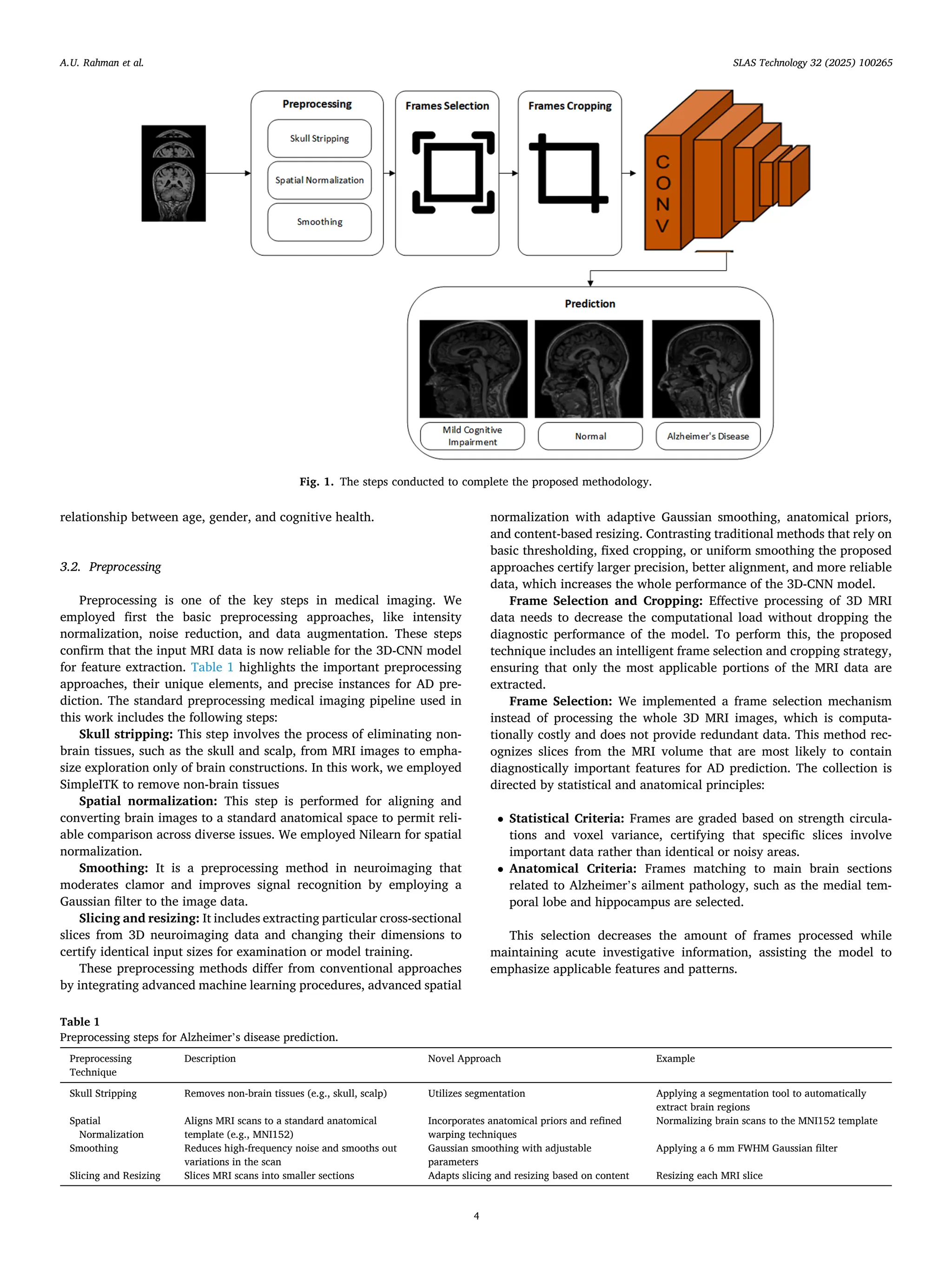
![Frame Cropping: The cropping step is employed to separate the
region of interest (ROI) within each frame after selecting the diagnos
tically applicable frames. This step has the subsequent elements:
• ROI Detection: Bounding boxes are produced near the brain area
using a segmentation procedure to eliminate inappropriate parts,
such as surrounding non-brain tissues and background.
• Standardized Cropping: Every nominated frame is cropped to a
fixed size (e.g., 128×128 pixels), ensuring consistency across the
dataset and decreasing computational overhead.
The cropping process improves the emphasis of the 3D-CNN model
on disease-specific features, refining its capacity to distinguish certain
patterns related to Alzheimer’s ailment.
Impact of Frame Selection and Cropping: The frame selection and
cropping procedures contribute to the model’s competency and
accuracy:
• Efficiency Gains: The computational time of training and testing is
considerably reduced by decreasing the number of frames and
concentrating on ROIs. This allows the usage of DL models with
larger datasets while utilizing limited resources.
• Improved Accuracy: Eliminating unrelated data ensures that the
model is exposed to learn only critical patterns more relevant to the
disease pattern, which improves the diagnostic accuracy of the
model.
The MRI data based on T1-Weighted in NIFTI format from the dataset
is preprocessed with the help of the CAT12 toolkit. This tool is provided
by the SPM12, which is a third-party MATLAB toolbox. The MRI images
were transformed to adhere to the dimensions of 121×145×121 (X × Y
× Z) with a spatial resolution of 1.5 × 1.5 × 1.5 mm3 per voxel.
Furthermore, all MRI images underwent signal intensity normalization,
where each voxel value was normalized by dividing it by the maximum
value of the MRI. The 3D-MRI data consisting of 121×145×121 di
mensions for transverse, sagittal, and coronal views were acquired
through re-slicing, resulting in dimensions of (145×121), (121×121),
and (121×145), respectively. Subsequently, edge padding and zero
filling were applied, and all 2D frames were resized to dimensions of
(145×145). The process of skull stripping involves the removal of non-
cerebral tissues such as the skull, scalp, and dura from brain images. One
method used for this purpose is Adaptive Probability Region-Growing
(APRG), which refines probability through region-growing methods
[45]. Currently, the APRG method is the most accurate and dependable
approach for skull removal in brain MRI data. In our research, we have
successfully employed the APRG method to eliminate the skull from the
MRI data.
The brains of humans exhibit variations in shapes among individuals.
One primary objective of spatial normalization is to deform the scans of
the brain in a way that aligns with a specific location. It involves
transforming images from different subjects into a common coordinate
system, ensuring that anatomically corresponding regions are in uni
form positions. Spatial normalization can be considered a specialized
form of image registration. Its purpose is to map an MRI image of an
individual onto the brain’s reference space, enabling comparisons be
tween subjects with diverse brain morphologies. In this work, DARTEL
registrations were utilized to achieve spatial registration. This involved
aligning the individual MRI images with an existing template, facili
tating the comparison of brain scans across subjects with varying brain
structures [46]. Smoothing is a technique for eliminating various types
of noise present in MRI frames. This study employed a Gaussian filter to
reduce noise in the MRI data.
A substantial number of frames per view, totaling nearly 150 frames
for each set of MRI images following preprocessing. This enormous
number of frames requires incredible processing resources to train a
CNN model. Furthermore, overfitting of the CNN may result from data
redundancy. Recently, various studies have used a random selection
technique to overcome this difficulty. More precisely, the study in [36]
used 33 transverse frames, 40 sagittal frames, and 50 coronal frames,
which were randomly selected, yielding 123 frames taken from a sub
ject’s 3D brain imagery. This decrease in the total number of frames
assists in reducing the computing requirements and any overfitting
difficulties that come with training a CNN model on such big datasets.
The proposed framework deployed an innovative frame selection
method. This approach recognizes and ranks parts that show robust
associations with Alzheimer’s pathology, efficiently decreasing noise
and computational time while conserving critical diagnostic facts.
However, it is hard to discover which frame has the most valuable in
formation, so randomly picking frames might not be compelling. This
random selection method might result in the loss of critical data. In our
research, we adopted a different strategy by choosing frames based on
statistical analysis. To begin, we calculated the number of informative
pixels using Eq (1). Frames with fewer informative pixels than the
threshold value were discarded.
I = 1 −
N0
HI × WI
(1)
The total number of zeros is represented by N0 in an image with the
height of HI the width of WI. In this study, the top 40 informative frames
from each view are chosen, leading to a total of 120 frames per patient in
the analysis. The frames that were selected based on statistical criteria
effectively lowered the computational complexity of MRI processing.
Each frame encompassed varying sizes of informative regions. To
establish an average window size for all patients across the three views,
we employed the proposed algorithm, referred to as Algorithm 1. The
computational complexity of the proposed model expressively reduced
after frame selection, with reductions of nearly 92 % in input data size,
87 % training time decrease, and 90 % lessening in inference time,
together with a 75 % reduction in GPU memory utilization. This high
lights the productivity of smart frame selection in enhancing resource
usage while stabilizing model presentation. Table 2 represents the
computational complexity comparison before and after frame selection
of the proposed model.
3.3. Model development
The proposed model is employed to capture the spatial and volu
metric features of MRI data widely. It includes improved layers for
deeper feature extraction and leverages a tailored learning rate opti
mization method for effectual training. Fig. 2 represents the architecture
of the proposed 3D-CNN model used in this study.
The proposed work has applied 3D architecture, in which a shallow
3D-CNN architecture, i.e., width × height × view × number_of_frames, is
proposed and compared with recent research that has used 3D-CNN for
the classification of AD [36]. The proposed 3D-CNN is used to capture
the information from all three views at the same time. In this study, a
shallow 3D-CNN architecture that is especially targeted towards classi
fying AD is proposed. This architecture is made to analyze
multi-dimensional data. By concurrently weighing data from several
points of view or vantage points, it aims to advance earlier studies and
produce more reliable and accurate results for the diagnosis of AD.
Input Layer: The MRI images are 3D volumetric data denoted as a
tensor X having a shape (D, H, W, C). Where D represents depth (number
of slices), H height of each slice, W width of the slice, and C number of
channels.
3D Convolution Layer: The convolution layer employs a 3D kernel
across the input data to create feature maps that maintain depth. The 3D
kernel K with shape (kd,kh,kw,C), the convolution operation is described
in Eq (2).
A.U. Rahman et al. SLAS Technology 32 (2025) 100265
5](https://image.slidesharecdn.com/25-250808164853-630173f6/75/25-Rahman-Alzheimer-s-disease-prediction-using-3D-CNNs-Intelligent-processing-of-neuroimaging-data-pdf-5-2048.jpg)
![Yi,j,k =
∑
C
c=1
∑
kd− 1
p=0
∑
kh− 1
q=0
∑
kw− 1
r=0
Xi+p,j+q,k+r,c⋅Kp,q,r,c + b (2)
Where Y shows the output feature map, (i, j, k) shows the position of
the feature map, and b is the bias term.
Activation Function: For introducing non-linearity to learn com
plex patterns in the MRI data, Rectified Linear Unit (ReLU) is applied. It
is defined as shown in Eq (3).
Y
ʹ
i,j,k = max
(
0, Yi,j,k
)
(3)
Where, Yi,j,k the represented the input to the activation function and
Y
ʹ
i,j,k indicate outputs as the input value, if it is positive otherwise 0 if the
input is negative, presenting non-linearity to the model.
3D Max Pooling: For preserving only the prominent features, max
pooling is used. It downsamples the feature maps by choosing only the
maximum value in the specific window. For the input Yʹ using a pooling
window P of size (pd,ph,pw), the pooling operation is described in Eq. (4).
Zi,j,k = max
0≤m<pd,0≤n<ph,0<o<pw
Yʹ
ipd+m,j.ph+n,k.pw+o
(4)
It mines the extreme value from a distinct 3D area of the input Yʹ,
decreasing its dimensions while recalling the most important features.
Fully Connected Layers: Using several convolutional and pooling
layers, the 3D feature is flattened into a 1D vector and passed to the fully
connected layers. It combines the high-level features from the entire
MRI image to perform the final predictions as discussed in Eq (5).
z(l+1)
= f
(
W(l)
z(l)
+ b(l)
)
(5)
Where z represents the flattened vector, the W(l)
represents weights
and biases of layer l is denoted by b(l)
, the input to the layer z(l)
. The
activation function is represented by f employed to z(l+1)
find the output
for the resulting layer.
Output Layer: For three class classifications, the softmax activation
function is used. It outputs the probability scores for each class as rep
resented in Eq (6).
Softmax(z) =
exp(zi)
∑
jexp
(
zj
) (6)
The input to the softmax function is a vector represented by (z) = [z1,
z2, …, zn], where each zi signifies the score for the ith
class in a classifi
cation tricky. The Softmax function used the exponential oper
ationexp(zi) for each sore each zi. The numerator exp(zi) is divided by
the summation of exponentials of all scores
∑
jexp
(
zj
)
.
4. Experiments
In this work, various experiments are conducted to assess the effec
tiveness of the proposed 3D-CNN architecture for the categorization of
AD. This work also focused on the 3D-CNN architectures to avoid the
model’s underfitting and overfitting problems. The architectures of 3D-
CNN are shown in Fig. 2, where C stands for the convolutional layer, P
for the pooling layer, and FC for the fully connected layer. The archi
tecture is shallow because of intelligent frame selection and cropping, as
compared to the literature. [47]. The proposed 3D-CNN model contains
a total number of learnable parameters are 1091,475, which shows its
complexity and volume for classification and feature extraction.
Algorithm 1
Skull stripping, smoothing, and frame selection.
Input: # number of images
Output: preprocessed image
For each image in the image list
Load the image
Skull stripping:
Use skull stripping algorithm to eliminate non-brain tissues
Save the skull-stripped image
Smoothing:
Use a smoothing algorithm to decrease noise
Save the smoothed image
Frame Selection:
Analyze the image content and motion to choose the frame
Save the selected frame
Save the results:
Save the preprocessed images
End loop
Table 2
Complexity comparison before and after frame selection.
Parameter Before After Reduction
(%)
Total frames 150 120 20
Input volume (reduction in
depth)
256×256×150 256×256×120 23
Memory usage (per batch) 629MB 409MB 35
Training time (per epoch) 3 h 2.43 h 19
Inference time (per epoch) 30 s 22.8 s 24
Fig. 2. The architecture of the proposed 3D-CNN model used in this study.
A.U. Rahman et al. SLAS Technology 32 (2025) 100265
6](https://image.slidesharecdn.com/25-250808164853-630173f6/75/25-Rahman-Alzheimer-s-disease-prediction-using-3D-CNNs-Intelligent-processing-of-neuroimaging-data-pdf-6-2048.jpg)
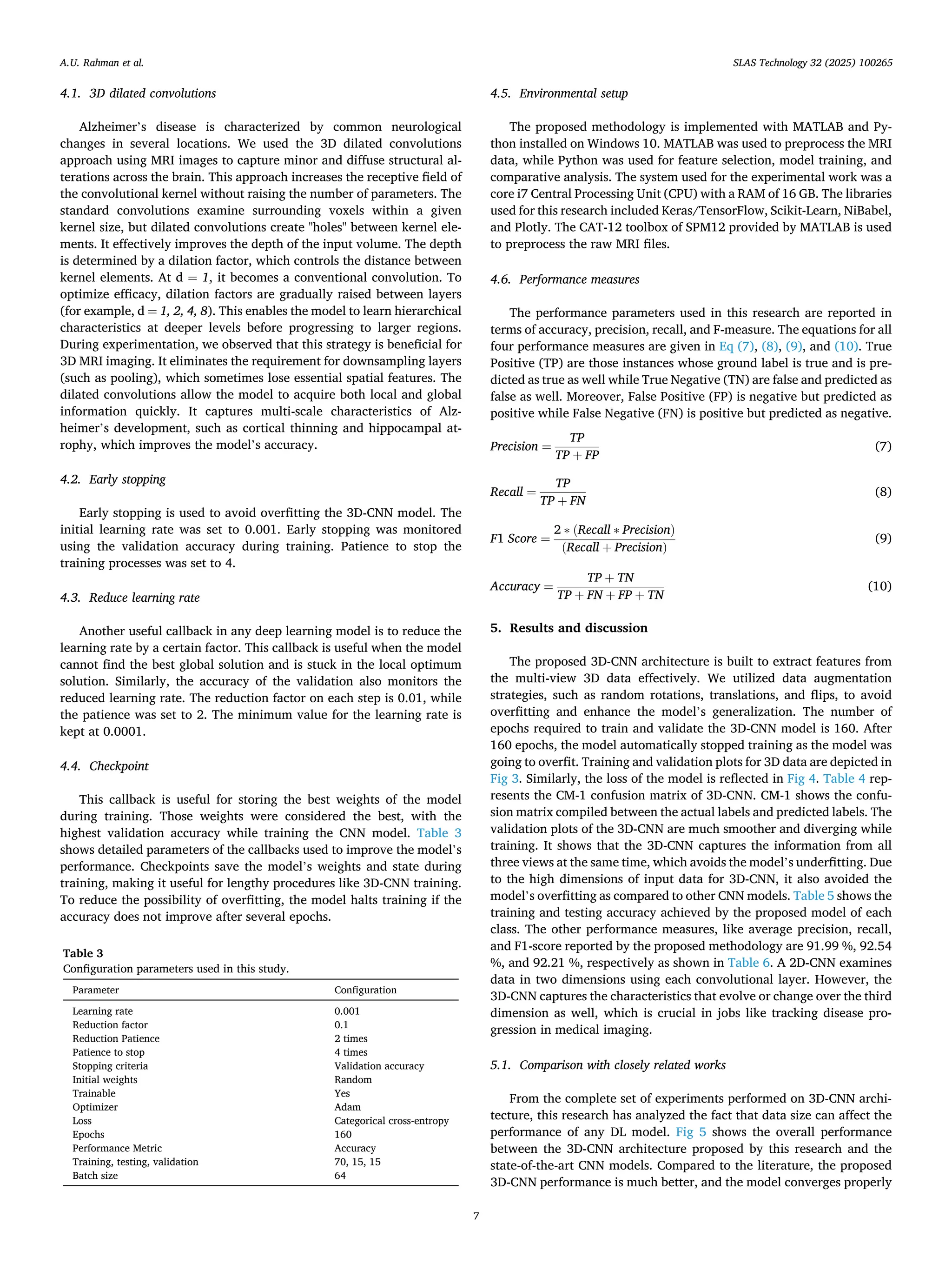
![because of the simultaneous extraction of features from data. The fitting
of CNN models depends on the number of learnable parameters in any
DL model. Table 7 depicts the overall comparison between the proposed
3D-CNN architecture and the most relevant literature. The authors in
[47] used 123 random frames selected from the input preprocessed data,
trained all the 123 2D models separately, and then took the average of
all the accuracies. It is observed that the number of parameters in [47]
has 1.227 M parameters, which is more than the 2D-CNN architecture
proposed by this research. The performance of the proposed model is
8+% greater than the literature [47]. Although the accuracy difference
between the proposed method and the transfer learning-based 2D
VGG-19, [37], is almost 5 %. However, the number of parameters in our
proposed method is 127 times less than their method, which is a great
achievement.
Moreover, the dataset size is almost 7 times less than the proposed
work selected dataset. The number of parameters is much higher than
ours and the dataset size is also very small as compared to the proposed
work. Thus, the experimental results reflect that the intelligent
Fig. 3. Training and testing accuracy of the proposed model.
Fig. 4. Training and testing loss of the proposed model.
Table 4
CM-1 confusion matrix of 3D-CNN.
CN MCI AD
CN 135 7 8
MCI 4 187 5
AD 3 4 83
Table 5
Accuracy achieved by the proposed model.
Class Training Accuracy (%) Testing Accuracy (%)
AD 92.38 90.15
CN 94.62 91.21
MCI 93.75 92.89
Average 93.58 91.41
Table 6
Results obtained using the proposed model.
Class Precision (%) Recall (%) F1-score (%)
AD 86.46 92.22 89.25
CN 95.07 90.00 92.47
MCI 94.44 95.41 94.92
Average 91.99 92.54 92.21
A.U. Rahman et al. SLAS Technology 32 (2025) 100265
8](https://image.slidesharecdn.com/25-250808164853-630173f6/75/25-Rahman-Alzheimer-s-disease-prediction-using-3D-CNNs-Intelligent-processing-of-neuroimaging-data-pdf-8-2048.jpg)
![preprocessing methods and frame selection approach improve the
model’s accuracy. Compared to current state-of-the-art works, the pro
posed 3D-CNN reached the highest accuracy of 92.89 % for AD
prediction.
5.2. Discussion
The 3D-CNN model used in this research has a much smaller number
of learnable parameters as compared to other relevant studies [36].
They performed various experiments and the best classification accuracy
the authors have reported is 84.57 %, which is 8 % less than the pro
posed 3D-CNN architecture used in this study. Moreover, the number of
subjects is just 988, which is quite low compared to our selected dataset.
The possible reason is that the number of parameters in the proposed
3D-CNN is almost 10 times less than the models used in the literature.
Similarly, [44] has used a much larger dataset size but their number of
parameters is greater than our proposed method while the accuracy is
less than ours. The authors have used 3D DenseNet-121 architecture for
training and prediction of the disease. Our proposed model performance
is almost 8 % greater than [44], and the reason is our intelligent frames
selection and cropping, and the simpler CNN architecture we have
proposed in this study. The study also emphasizes how effective model
architecture and data size affect DL models’ overall effectiveness. The
suggested model expands the potential for precise and effective AD
diagnosis and progressing monitoring by attaining competitive precision
outcomes with fewer parameters. (Table 8)
We conducted an ablation study to assess the influence of each factor
in the proposed 3D-CNN model. The study thoroughly examined various
components, like preprocessing steps, the frame selection scheme, and
particular CNN layers, to measure their distinct effect on the model’s
operations. This conveys critical intuitions into the implication of each
element in the proposed model. The complete model, which contains
preprocessing, frame selection, and all CNN layers along with 3D dila
tion, achieves the highest accuracy (92.89 %) and F1 score (92.21 %).
This configuration shows the model’s capacity to balance computational
time and diagnostic performance efficiently. The accuracy and F1-score
drop to 87.2 % and 85.7 %, respectively when preprocessing is omitted,
despite a minor reduction in computational time. This highlights the
significance of preprocessing in improving input data quality and
enabling better feature extraction. Similarly, eliminating frame selection
decreases the model’s accuracy to 89.8 % and F1-score to 87.5 %. This
consequence approves the critical role of preprocessing, and frame se
lection in removing inappropriate frames and concentrating on focused
areas, which decreases noise and enhances model accuracy.
6. Conclusions
This work developed a novel preprocessing, intelligent frame selec
tion, and 3D-CNN based approach for AD prediction. During the
experimentation, we observed that CNNs are highly dependent on the
input data. If the data is clean and informative, and the model will
extract large amounts of information, it will produce better results. This
research has concluded this phenomenon through various experimental
results. We also observed that, training on the less informative data
results in the overfitting of CNN architectures. Similarly, a CNN with
more learnable parameters will take more time to learn, also sometimes
will lead to overfitting and vice versa. In the case of 2D-CNN, it extracts
Fig. 5. Results comparison with closely related works.
Table 7
Results comparison with state-of-the-art works.
Author Architecture Subjects Parameters No of
Models
Accuracy
(%)
[47] 2D-CNN 509 1227,731 123 84.05
[37] 2D VGG-19 300 138,423,208 1 87.15
[36] 3D-CNN 988 10,467,315 1 84.57
[44] 3D DenseNet-
121
3512 7628,484 1 84.00
Proposed 3D-CNN 2186 1091,475 1 92.89
Table 8
Ablation study results of the proposed model.
Configuration Preprocessing Frame
Selection
Accuracy
(%)
F1-Score
(%)
Full Model Yes Yes 92.89 92.21
Without
Preprocessing
No Yes 87.2 85.7
Without Frame
Selection
Yes No 89.8 87.5
Reducing
Convolutional
Layers
Yes Yes 88.1 86.9
A.U. Rahman et al. SLAS Technology 32 (2025) 100265
9](https://image.slidesharecdn.com/25-250808164853-630173f6/75/25-Rahman-Alzheimer-s-disease-prediction-using-3D-CNNs-Intelligent-processing-of-neuroimaging-data-pdf-9-2048.jpg)
![features limited to 2D spatial domains, often lacking volumetric patterns
like atrophy in brain regions, which span across 3D spaces. It ignores the
depth, which results in the loss of inter-slice spatial information. We also
observed that the 2D-CNN requires slice stacking, or recurrent layers, to
address the volumetric information in MRI images. However, the 3D-
CNN captures hierarchical information over the whole 3D space, mak
ing it more effective at recognizing scattered and subtle changes in brain
MRI images. Also, applying 3D dilated convolution, enabled the model
to receive a larger receptive field inherently across all three dimensions,
supporting more efficient global and local feature extraction.
In the future, we want to employ transfer learning, like using pre-
trained models on 3D imaging datasets (e.g., MedicalNet) and fine-
tuning them on the ADNI dataset to utilize learned representations.
CRediT authorship contribution statement
Atta Ur Rahman: Writing – original draft, Software, Methodology,
Conceptualization. Sania Ali: Writing – review & editing, Software,
Data curation. Bibi Saqia: Methodology, Investigation, Formal analysis.
Zahid Halim: Validation, Software, Resources. M.A. Al-Khasawneh:
Resources, Formal analysis, Data curation. Dina Abdulaziz AlHam
madi: Validation, Resources, Investigation. Muhammad Zubair Khan:
Visualization, Resources, Formal analysis. Inam Ullah: Writing – review
& editing, Supervision, Resources, Project administration, Funding
acquisition. Meshal Alharbi: Data curation, Formal analysis, Resources.
Declaration of competing interest
The authors declare that they have no known competing financial
interests or personal relationships that could have appeared to influence
the work reported in this paper.
References
[1] Tufail AB, et al. 3D convolutional neural networks-based multiclass classification of
Alzheimer’s and Parkinson’s diseases using PET and SPECT neuroimaging
modalities. Brain Inform 2021;8:1–9.
[2] Breijyeh Z, Karaman R. Comprehensive review on Alzheimer’s disease: causes and
treatment. Molecules 2020;25(24):5789.
[3] Wang X, Qi J, Yang Y, Yang P. A survey of disease progression modeling techniques
for alzheimer’s diseases. In: 2019 IEEE 17th International Conference on Industrial
Informatics (INDIN). 1. IEEE; 2019. p. 1237–42.
[4] Fabrizio C, Termine A, Caltagirone C, Sancesario G. Artificial intelligence for
Alzheimer’s disease: promise or challenge? Diagnostics 2021;11(8):1473.
[5] Mishra R, Li B. The application of artificial intelligence in the genetic study of
Alzheimer’s disease. Aging Dis 2020;11(6):1567.
[6] Vrahatis AG, Skolariki K, Krokidis MG, Lazaros K, Exarchos TP, Vlamos P.
Revolutionizing the early detection of Alzheimer’s disease through non-invasive
biomarkers: the role of artificial intelligence and deep learning. Sensors 2023;23
(9):4184.
[7] King A, Bodi I, Troakes C. The neuropathological diagnosis of Alzheimer’s
disease—The challenges of pathological mimics and concomitant pathology. Brain
Sci 2020;10(8):479.
[8] Almohimeed A, et al. Explainable artificial intelligence of multi-level stacking
ensemble for detection of Alzheimer’s disease based on particle swarm
optimization and the sub-scores of cognitive biomarkers. IEEE Access 2023.
[9] Hao X, et al. Multimodal self-paced locality-preserving learning for diagnosis of
Alzheimer’s disease. EEE Transac Cognit Developm Syst 2022;15(2):832–43.
[10] Chui KT, Gupta BB, Alhalabi W, Alzahrani FS. An MRI scans-based Alzheimer’s
disease detection via convolutional neural network and transfer learning.
Diagnostics 2022;12(7):1531.
[11] Ledig C, Schuh A, Guerrero R, Heckemann RA, Rueckert D. Structural brain
imaging in Alzheimer’s disease and mild cognitive impairment: biomarker analysis
and shared morphometry database. Sci Rep 2018;8(1):11258.
[12] Zhao X, Ang CKE, Acharya UR, Cheong KH. Application of Artificial Intelligence
techniques for the detection of Alzheimer’s disease using structural MRI images.
Biocybernet Biomed Eng 2021;41(2):456–73.
[13] Rasheed Z, et al. Automated classification of brain tumors from magnetic
resonance imaging using deep learning. Brain Sci 2023;13(4):602.
[14] Leandrou S, Petroudi S, Kyriacou PA, Reyes-Aldasoro CC, Pattichis CS.
Quantitative MRI brain studies in mild cognitive impairment and Alzheimer’s
disease: a methodological review. IEEE Rev Biomed Eng 2018;11:97–111.
[15] Rasheed Z, Ma Y-K, Ullah I, Al-Khasawneh M, Almutairi SS, Abohashrh M.
Integrating convolutional neural networks with attention mechanisms for Magnetic
resonance imaging-based classification of brain tumors. Bioengineering 2024;11
(7):701.
[16] Zhao Y, et al. Application of deep learning for prediction of alzheimer’s disease in
PET/MR imaging. Bioengineering 2023;10(10):1120.
[17] Kale MB, et al. AI-driven innovations in Alzheimer’s Disease: integrating early
diagnosis, personalized treatment, and prognostic modelling. Ageing Res. Rev.
2024:102497.
[18] Fan C-C, et al. Graph reasoning module for Alzheimer’s Disease diagnosis: a plug-
and-play method. IEEE Transac Neural Syst Rehabilit Eng 2023;31:4773–80.
[19] Basher A, Kim BC, Lee KH, Jung HY. Volumetric feature-based Alzheimer’s disease
diagnosis from sMRI data using a convolutional neural network and a deep neural
network. IEEE Access 2021;9:29870–82.
[20] Hinrichs C, et al. Spatially augmented LPboosting for AD classification with
evaluations on the ADNI dataset. Neuroimage 2009;48(1):138–49.
[21] Terry RD. Alzheimer’s disease and the aging brain. J Geriatr Psychiatry Neurol
2006;19(3):125–8.
[22] Sharma S, Mandal PK. A comprehensive report on machine learning-based early
detection of alzheimer’s disease using multi-modal neuroimaging data. ACM
Comput Surveys (CSUR) 2022;55(2):1–44.
[23] Ahmed MJ, et al. CardioGuard: aI-driven ECG authentication hybrid neural
network for predictive health monitoring in telehealth systems. SLAS Technol
2024;29(5):100193.
[24] Rathore S, Habes M, Iftikhar MA, Shacklett A, Davatzikos C. A review on
neuroimaging-based classification studies and associated feature extraction
methods for Alzheimer’s disease and its prodromal stages. NeuroImage 2017;155:
530–48.
[25] Moradi E, Pepe A, Gaser C, Huttunen H, Tohka J, Initiative AsDN. Machine
learning framework for early MRI-based Alzheimer’s conversion prediction in MCI
subjects. Neuroimage 2015;104:398–412.
[26] Ebrahimighahnavieh MA, Luo S, Chiong R. Deep learning to detect Alzheimer’s
disease from neuroimaging: a systematic literature review. Comput Methods
Programs Biomed 2020;187:105242.
[27] Tufail AB, et al. On disharmony in batch normalization and dropout methods for
early categorization of Alzheimer’s disease. Sustainability 2022;14(22):14695.
[28] Mohi ud din dar G, et al. A novel framework for classification of different
Alzheimer’s disease stages using CNN model. Electronics 2023;12(2):469.
[29] Ebrahimi A, Luo S, Disease Neuroimaging Initiative ftAs. Convolutional neural
networks for Alzheimer’s disease detection on MRI images. J Med Imag 2021;8(2).
024503-024503.
[30] Cui R, Liu M, Initiative AsDN. RNN-based longitudinal analysis for diagnosis of
Alzheimer’s disease. Computer Med Imag Graph 2019;73:1–10.
[31] Vincent P, Larochelle H, Lajoie I, Bengio Y, Manzagol P-A, Bottou L. Stacked
denoising autoencoders: learning useful representations in a deep network with a
local denoising criterion. J Mach Learn Res 2010;11(12).
[32] Hinton GE. Deep belief networks. Scholarpedia 2009;4(5):5947.
[33] Sharma M, Sharma P, Pachori RB, Acharya UR. Dual-tree complex wavelet
transform-based features for automated alcoholism identification. Int J Fuzzy Syst
2018;20(4):1297–308.
[34] Farooq A, Anwar S, Awais M, Rehman S. A deep CNN based multi-class
classification of Alzheimer’s disease using MRI. In: 2017 IEEE International
Conference on Imaging systems and techniques (IST). IEEE; 2017. p. 1–6.
[35] Haarburger C, et al. Multi scale curriculum CNN for context-aware breast MRI
malignancy classification. In: International Conference on Medical Image
Computing and Computer-Assisted Intervention. Springer; 2019. p. 495–503.
[36] Khagi B, Kwon G-R. 3D CNN design for the classification of Alzheimer’s disease
using brain MRI and PET. IEEE Access 2020;8:217830–47.
[37] Mehmood A, et al. A transfer learning approach for early diagnosis of Alzheimer’s
disease on MRI images. Neuroscience 2021;460:43–52.
[38] Acharya RMH, Singh DK. Alzheimer Disease classification using transfer learning.
In: 5th International Conference on Computing Methodologies and Communication
(ICCMC); 2021. p. 1503–8.
[39] Deepak S, Ameer P. Automated categorization of brain tumor from mri using cnn
features and svm. J Ambient Intell Humaniz Comput 2021;12(8):8357–69.
[40] Shakarami A, Tarrah H, Mahdavi-Hormat A. A CAD system for diagnosing
Alzheimer’s disease using 2D slices and an improved AlexNet-SVM method. Optik
(Stuttg) 2020;212:164237.
[41] Ebrahim D, Ali-Eldin AM, Moustafa HE, Arafat H. Alzheimer disease early
detection using convolutional neural networks. In: 2020 15th international
conference on computer engineering and systems (ICCES). IEEE; 2020. p. 1–6.
[42] Odusami M, Maskeliūnas R, Damaševičius R, Krilavičius T. Analysis of features of
alzheimer’s disease: detection of early stage from functional brain changes in
magnetic resonance images using a finetuned ResNet18 network. Diagnostics 2021;
11(6):1071.
[43] Buvaneswari P, Gayathri R. Deep learning-based segmentation in classification of
Alzheimer’s disease. Arabian J Sci Eng 2021;46(6):5373–83.
[44] Solano-Rojas B, Villalón-Fonseca R, Marín-Raventós G. Alzheimer’s disease early
detection using a low cost three-dimensional densenet-121 architecture. In:
International conference on smart homes and health telematics. Springer; 2020.
p. 3–15.
[45] Toennies RPaKD. Segmentation of medical images using adaptive region growing.
Med Imag; Image Process 2017:1337–46.
[46] Ashburner J. A fast diffeomorphic image registration algorithm. Neuroimage 2007;
38:95–113.
[47] Pan AZD, Jia L, Huang Y, Frizzell T, Song X. Early detection of Alzheimer’s disease
using magnetic resonance imaging: a novel approach combining convolutional
neural networks and ensemble learning. Front Neurosci 2020;14.
A.U. Rahman et al. SLAS Technology 32 (2025) 100265
10](https://image.slidesharecdn.com/25-250808164853-630173f6/75/25-Rahman-Alzheimer-s-disease-prediction-using-3D-CNNs-Intelligent-processing-of-neuroimaging-data-pdf-10-2048.jpg)


![[DSC Europe 25] Uros Pesic - The Reality of AI in Marketing.pdf](https://cdn.slidesharecdn.com/ss_thumbnails/rtkodnmtycovsllvzsyn-9-251215095918-b0c6bfe3-thumbnail.jpg?width=640&height=640&fit=bounds)
![[DSC Europe 25] Dunja Adzic Jovanovic - AI and Cybersecurity: Defending Data ...](https://cdn.slidesharecdn.com/ss_thumbnails/o1zylpbhrtwnixxq2xj8-7-251211083048-185086f6-thumbnail.jpg?width=640&height=640&fit=bounds)
![[DSC Europe 25] Branko Urosevic -Rethinking Financial Talent: Integrating Cod...](https://cdn.slidesharecdn.com/ss_thumbnails/8jjrus8ttko6qj64f58f-3-251212103250-642c6374-thumbnail.jpg?width=640&height=640&fit=bounds)


![[DSC Europe 25] Miodrag Pesovic & Vladislav Radonjic - Federated Data Archite...](https://cdn.slidesharecdn.com/ss_thumbnails/gsbe3y5it5uhndi4e08e-1-251212103249-f1008e0c-thumbnail.jpg?width=640&height=640&fit=bounds)
![[DSC Europe 25] Nikolay Burlutskiy - Best Practices for Building Enterprise M...](https://cdn.slidesharecdn.com/ss_thumbnails/uirvaiuvq8y1w8hzd9tx-7-251212103249-2619edb4-thumbnail.jpg?width=640&height=640&fit=bounds)


![[DSC Europe 25] Jon Dajci - Bridging TradFi and DeFi: Building the Future of ...](https://cdn.slidesharecdn.com/ss_thumbnails/fqmhfvlbqhkihjvqvhmu-7-251211083849-6af7e325-thumbnail.jpg?width=640&height=640&fit=bounds)


![[DSC Europe 25] Branko Dzakula - From Defense to Attack: How AI Redefines Cyb...](https://cdn.slidesharecdn.com/ss_thumbnails/80bdzdxpr3ky2g0qvyk9-8-251211083048-ce5fc1ee-thumbnail.jpg?width=640&height=640&fit=bounds)

![[DSC Europe 25] Katherine Forrest - AI NOW: Understanding the Velocity of Cha...](https://cdn.slidesharecdn.com/ss_thumbnails/wvvbruqfrci0sfq9xwgb-4-251212104007-e5ad1987-thumbnail.jpg?width=640&height=640&fit=bounds)
