SlideShare a Scribd company logo
1 of 34
Download to read offline
The Causes of Declining Residential Water Sales
A Research Report for the Louisville Water Company
by
Paul Coomes, Ph.D.
Professor of Economics, and
National City Research Fellow
Margaret Maginnis, Senior Research Associate
Fadden Holden, Economics Student
University of Louisville
December 2005
Executive Summary
he Louisville Water Company has been experiencing declining water sales among
residential customers, forcing the company to raise rates to ensure the revenues
needed to expand service and replace old water mains and equipment. Water use per
residential customer in both 2003 and 2004 was the lowest on record, twenty percent lower
than the usage peak in 1988. Company officials attribute the decline in usage to several
possible factors including wetter weather, new water-conserving appliances, changing
demographics, and classification anomalies.
T
We have studied the academic and industrial literature and examined historical data on water
usage in order to better understand the causes of declining water use by households in the
service area. In addition, we have examined the Company’s customer database to ascertain
the extent to which classification procedures miss residential demand in multi-family
complexes. We also fit an econometric model, using thirty years of monthly residential water
use per customer, to obtain indications of the importance of key variables in causing the
decline in water use.
The empirical literature suggests that there is a positive relationship between household size
and water usage. However, it also indicates that water use does not increase proportionately
with number of persons due to economies of scale in dishwashing, laundry and other
common functions. Thus, played in reverse, as the average number of persons per
household declines in the Louisville market, there will be a reduction in water use per
household, but at a diminishing rate. Our preliminary econometric work suggests that at least
one-third of the decline in residential water use over the last fifteen years is due to a
reduction in the number of persons per household. Our model also suggests that water usage
per person has remained fairly stable over the last thirty years, so that declining household
demand is a function of less people per household rather than less individual water use.
There have been dozens of studies published that examine the sensitivity of residential water
usage to price increases and decreases. While there are a wide range of estimates reported,
they cluster most around a price elasticity of demand of -0.4 to -0.5, with outdoor water use
much more price-sensitive than indoor use. Given that water is a necessity of life, it is not
surprising that overall demand is inelastic. A policy consequence of this finding is that the
Louisville Water Company could raise water rates significantly without a proportionate
decrease in sales, stimulating Company revenues as needed. Specifically, assuming this
midpoint estimate of elasticity, a twenty percent increase in rates would lead to a ten percent
decrease in residential water sales per customer. Company revenues would rise even though
less water would be provided to the customers. A complicating issue is that the sewer bill,
also based on water usage, is presented to customers jointly with the water bill. Hence, when
the Metropolitan Sewer District raises its sewer charges, customers see this as an increase in
water rates. Were water and sewer rates to creep up over time, and the bi-monthly bill
become high enough that residential customers start to notice the impact on their budgets,
customers would likely become more price-sensitive.
The American Water Works Association has sponsored a very useful study of end uses of
water by households that provides detailed data on water use by indoor appliances and
outdoor usage. Although the study was conducted primarily in far western and southern
cities across the United States, the methodology can be directly applied to Louisville, with
some of their results transferable as well. We recommend a local end use study, whereby
electronic data loggers are installed on the meters of a small sample of Louisville households.
Water usage by appliance can then be modeled against measures of household technology
along with demographic and economic factors. We believe this is the most promising and
cost-effective way to finally determine the impact of new water-conserving appliances and to
distinguish between indoor and outdoor water use.
Since the objective of our research was to understand residential water usage in Louisville,
we were curious about how many households were not classified as residential customers.
Because of state tax laws and some legacy information technology issues, most apartments
and other multi-family units are classified as commercial customers, and hence their water
usage is not included in the residential data we examined. We investigated this issue in great
detail, using a random sample of 500 commercial customers. We found that the sample
include 162 premises containing 1,528 housing units. We can infer from this that, county-
wide, there are nearly 44,200 housing units currently counted under the commercial
classification. If the Company wants to better understand household water demand, it needs
to reclassify these customers and track their usage separately from commercial customers. As
part of the sampling exercise we also found a number of single-family homes classified as
commercial customers. This suggests a need to clean the Company’s customer database so
that it is more useful for analytical purposes.
We believe the Company’s customer database is a rich and relatively untapped resource for
analysis of water usage patterns and trends. Much could be learned from matching customer
water use to geographic and economic data from other publicly available administrative data.
The LOJIC system can be used to determine the footprint of a housing unit, the lot size, and
whether a swimming pool is present. The lot size is a good indicator of sprinkler water usage
during droughts and the presence of a swimming pool is obviously an important explanatory
variable for outdoor water use. Customers with and without a separate meter for outdoor
water use can be studied, with these important controls for yard size and swimming pools.
Property Valuation Assessment records can be used to determine the age of a dwelling (an
indicator of its plumbing technology) and the assessed value (an indicator of household
income). Combined with results from regular end use studies discussed above, the Company
could effectively zoom in on the causes of trends and fluctuations in residential water use.
Residential Water Sales, Louisville Water Company 2
Overview of the Puzzle
ur team at the University of Louisville was engaged over the summer by the
Louisville Water Company to study the causes of recent decline in residential water
use per customer. Residential water usage per customer has fallen as the number of
residents and households continues to grow, and as household incomes continue to rise. The
chart below summarizes thirty years of monthly data on average water usage per residential
customer. A 12-month moving average was constructed to smooth out variations in month-
to-month use due to seasonal demand and billing anomalies. It is clear that water use per
customer has fallen significantly. Water usage peaked in late 1988 at around 7,000 gallons per
month. Today, the average customer uses only 5,600 gallons per month, a decline of 20
percent from the peak. This has serious revenue implications for the Louisville Water
Company. Stable revenues are needed to finance the capital programs required for replacing
legacy water mains and extending water service to new suburban communities. Increased
water rates are the most direct way to recoup revenues from falling water usage, but if the
Company continues to raise water rates there will eventually be resistance from homeowners
and voters. It has become increasingly urgent to understand what is causing the decline in
residential water sales.
O
Water Usage per Residential Customer
gallons by month, 1975-2004
4,000
5,000
6,000
7,000
8,000
9,000
10,000
11,000
Jun-75
Jun-76
Jun-77
Jun-78
Jun-79
Jun-80
Jun-81
Jun-82
Jun-83
Jun-84
Jun-85
Jun-86
Jun-87
Jun-88
Jun-89
Jun-90
Jun-91
Jun-92
Jun-93
Jun-94
Jun-95
Jun-96
Jun-97
Jun-98
Jun-99
Jun-00
Jun-01
Jun-02
Jun-03
Jun-04
12-month centered moving average
Several hypotheses have been advanced to explain the reduction in residential water usage.
1. Wetter weather has reduced the need for outdoor watering. There is a clear negative
relationship overall between rainfall and water usage per customer. The peak water
usage period (1988) in the chart above was among the driest in thirty years. The
relationship between average residential water usage and ground moisture is clear in
the chart below. We focus here only on the April to September months, when
outdoor watering of lawns and landscaping is most prevalent. The Palmer Drought
Residential Water Sales, Louisville Water Company 3
Severity Index provides a general measure of ground moisture for the central
Kentucky region. One can easily see the negative relationship between ground
moisture and residential water usage. The driest years, 1986 and 1988, were the ones
with the highest water usage. The wettest years, including the last two years, have low
water usage. We investigate this more carefully with an econometric model presented
later in this report.
2. The average number of persons per household has been falling, thereby reducing the
total water usage of the typical household. It is certainly true that the number of
persons per household has been falling in Jefferson County. The last four decennial
censuses revealed a decline from 3.16 persons per household in 1970, to 2.69 in
1980, to 2.48 in 1990, and to 2.37 in 2000. This represents a twenty-five percent
reduction in household size in just three decades. Industry research shows that water
usage is indeed sensitive to household size, as less people means less laundry, less
dishwashing, less bathing, and less toilet use per household. Our econometric work,
as well as the research of others, suggests that an additional person in a household
leads to between 600 and 1,100 gallons more water usage per month (depending on
age). Played in reverse and applied to the local situation, a drop in average household
size in Jefferson County from 2.92 to 2.35 persons during the 1975 to 2004 period,
would lead to a decline in monthly water usage of between 340 to 630 gallons per
residential customer. This range nicely brackets the actual net decline in average usage
(525 gallons per month per customer) seen by the Louisville Water Company over
the period. However, note from the first chart above that all of the decline in water
usage per customer has occurred since 1985, while household size has been falling
for decades. So, while falling household size has no doubt contributed greatly to
declining water sales, it is evidently not the only causal factor. Something else was
Average Residential Water Use vs. Ground Moisture Index
April to September, 1975 - 2004
30,000
35,000
40,000
45,000
50,000
-5 -4 -3 -2 -1 0 1 2 3 4 5
Palmer Drought Severity Index (-5 severe drought, +5 saturated), April to September only
AverageResidentialWaterUsage
2000
1999
1988
2004
1975
2003
1989
1986
1979
Residential Water Sales, Louisville Water Company 4
causing water usage per customer to rise in the earlier period even as there were
fewer people per household each year.
3. Federal water-conservation laws have required manufacturers to make water
appliances that use much less water, beginning in the mid-1990s. Most major
plumbing ware manufacturers began in 1994 to produce low-volume toilets, urinals,
showerheads, and faucets that comply with the Energy Policy Act of 1992
regulations1
. Thus, contractors have been installing low-flow water appliances in new
homes and in renovation projects for a decade now. These new appliances use on
net less than half the water per use as older appliances, though it is unclear how much
of this decline is offset by longer showers, multiple flushes, and second rinses in the
clothes washer. The Louisville area has seen a surge in home construction, and
Jefferson County has added 50,000 new housing units since 1990, accounting for
over one-sixth of the current housing stock. The chart below shows the distribution
of new housing (authorized) among single-family and multi-family units. Declining
interest rates have particularly spurred single-family home construction since the
early 1990s.
An end use modeling system would be required to understand the importance of the
new water-conserving appliances on water usage by household. Data loggers would
need to be installed on water meters in a sample of homes, with profiles developed
on the physical characteristics of the home and the demographic and economic
characteristics of the people living in the home. By controlling for these many
factors, analysts could determine the incremental effects of low-flow toilets, showers,
dishwashers, and clothes washers on the household’s water usage.
Housing Units Authorized, Single and Multi-Family
Jefferson County, Kentucky
1,694 1,669 1,590 1,684
1,869
2,266
2,714 2,799
2,480 2,567 2,508
3,087 3,027
2,797
2,978
2,749
3,164 3,237
1,681
1,120
738
762 537
637
343
855
627
871
480
1,026
1,323
1,012 599
761
831 649
0
500
1,000
1,500
2,000
2,500
3,000
3,500
4,000
4,500
5,000
1987 1988 1989 1990 1991 1992 1993 1994 1995 1996 1997 1998 1999 2000 2001 2002 2003 2004
Source: US Census Bureau.
Multi-Family Units
Single-Family Units
1
Source: letter from Amy Vickers and Associates to CH2M Hill Engineering, September 20, 1994.
Residential Water Sales, Louisville Water Company 5
Without an end-use study, we have only aggregate data on which to base estimates of
the effects of the new water-conserving appliances. In the econometric work
presented later, we develop a proxy for the introduction of water-conserving
appliances in the mid-1990s. Basically, we assume that all new homes are equipped
with lower-flow appliances and measure their rising share of the County’s total
housing stock. This measure, while admittedly crude, is statistically significant in one
model developed to explain the reduction in average water use among residential
customers.
4. A large proportion of households are classified as commercial water users in the
Water Company’s database. These households include apartment dwellers and condo
owners. We have extensively investigated this classification issue, using a random
sample of 500 Louisville Water Company ‘commercial’ customers in 2004. We found
that the sample included 162 residential premises, containing 1,528 housing units.
The sample results were adjusted for occupancy and applied to a County-wide
estimate, suggesting there are 44,200 occupied housing units in the County counted
under the commercial customer classification. This represents about one-sixth of all
occupied housing units (of any type) in Jefferson County. A detailed discussion of
our investigation is provided later in this report.
It is revealing to examine the growth in residential water customers and housing
units in Jefferson County between the last two decennial censuses. There is a tight fit
between the net growth in residential water customers and occupied housing units in
the County. Between 1990 and 2000, the Water Company gained 26,400 customers
classified as residential (from 193,400 to 220,800 customers). The Census Bureau
reports a growth of 23,800 occupied housing units over the decade (from 264,200 to
New Housing vs. Growth in Residential Water Customers
0
1,000
2,000
3,000
4,000
5,000
6,000
1988 1989 1990 1991 1992 1993 1994 1995 1996 1997 1998 1999 2000 2001 2002 2003 2004
Annual growth in residential water
customers, December to December
New housing units authorized in Jefferson
County, single and multi-family
287,000 units). The Census figure includes both owner-occupied and renter-occupied
Residential Water Sales, Louisville Water Company 6
housing units (186,400 and 100,600 respectively in 2000), but the Census does not
provide a breakout for single-family versus multi-family.
Annual building permit data follow the same general pattern as new residential
ere
e
ote that if one adds the number of average residential water customers (237,800) in
he
y
ounting apartment units as commercial customers causes a reduction in measured
er of
uilding permit records indicate that there are on average about 700 multi-family
l
ther water utilities around the United States are also now facing a decline in residential
ts of
,
water’s low price, and modest population growth.
customers, though the cumulative numbers do not align2
. The data show that th
were 25,000 new single-family homes authorized over the decade, plus 7,500 new
multi-family units. So, it appears that about 6,000 more units were built than can b
accounted for by the net growth in residential customers or occupied units. Much of
this discrepancy is due to demolitions, particularly around the airport and in older
neighborhoods west of Interstate 65.
N
the year 2004 to our estimate of occupied housing units classified as commercial
customers (44,200), you arrive at 282,000, only three percent less than the Census
Bureau’s estimate of the number of households (292,300) in Jefferson County for t
same year. The difference could be due to a higher occupancy rate for apartment
units than we assumed (90 percent), to sampling error, or to other Water Compan
classification issues.
C
residential customers, but also a biased measure of water usage per residential
customer – at least in the literal sense of the word residential. The average numb
persons living in a rental unit is less than in an owner-occupied dwelling. The 2000
Census reports 2.14 persons per rental unit versus 2.50 persons per owner-occupied
unit in Jefferson County. Given that fewer persons per unit translates directly into
lower water use per unit, we can infer that if all the multi-family housing units were
counted as residential customers, residential usage per customer across the system
would be even lower than now perceived.
B
units (apartments or condominiums) built in Jefferson County each year. Nearly al
of these households continue to be classified as commercial customers. The mixing
of households between the residential and commercial classifications makes an
analysis of household water usage more difficult.
O
water use per customer, and industry analysts are beginning to focus on the causes.
However, as will become evident in the next section, the literature on the determinan
household water usage is not very mature. Estimates vary widely of the effect of changing
household size, of conservation laws, and of the response to price and income increases.
Moreover, most of the relevant research has focused on water usage in the arid Southwest
where water rationing is a common occurrence. The paucity of research on household water
usage in the Midwest is no doubt due to the region’s historically ubiquitous water supply,
2
The three spikes in the chart showing growth of residential water customers are due to the conversion of
wholesale customers into residential customers – Jeffersontown (1990), Bullitt Kentucky Turnpike #2
(2000), and Goshen and Shepherdsville in 2002-03.
Residential Water Sales, Louisville Water Company 7
Review of Industry and Academic Research on
Residential Water Usage Modeling
n this section, we provide a summary of the published literature on residential water
usage. We have scoured industry and academic sources to identify any studies that have
looked at the issue of fluctuating water demand, with particular emphasis on quantifying
the factors that cause households to consume more or less water over time. The literature
provides some studies that help us understand what is causing the decline in average
residential water use in Louisville. Many variables have been used to fit demand models over
the last century, including water price, household income, outdoor water use, weather, and
household size. The dissemination of low-flow water appliances, prompted by the Energy
Policy Act of 1992, has spurred a fresh literature that focuses on water technology as a
variable also. A complete list of the studies cited is provided in a reference section at the end
of this report.
There are two basic methods used to analyze household water usage, econometric and end-
use. Econometric models have been fit using historical data on aggregate residential water
use for a system or for usage by individual households at a point in time or across time.
Residential water usage per customer by month is modeled as a function of weather, water
price, household demographics, technology, and other economic-demographic factors.
These models are also essentially models of shifting demand. Water supply is taken to be
inelastic at the given water price, regardless of quantity consumed. The quantity of water
demanded by a household may be price-sensitive at very high prices per gallon, but is quite
inelastic over the range of prices seen historically in the Midwest. That is, a rise in water
price of ten to twenty percent would not cause residences to use much less water. And a
similar drop in water prices would not cause residences to use much more water. The actual
water demand, and hence usage, in a market is determined by how weather and other factors
shift the demand curve, not by water prices.
The textbook supply and demand diagram above is useful as a conceptual starting point
only. The market for water is more complex, particularly when considering changes over
time. As with gasoline, electricity, medicine, and other necessities of life, demand for water
I
gallons of water
per month
$15
6,000
Price per
thousand
gallons
Supply
Demand
Residential Water Sales, Louisville Water Company 8
will certainly be more price-sensitive once consumers have a period to adjust. In the short-
onths), consum their housing
r
term (m
characteristics and lifestyles cannot be changed immediately. But over several years, people
would respond to higher water rates by installing more efficient appliances, fixing leaky
fixtures, and reducing outdoor watering. Moreover, the supply curve is not fixed over time.
The technology of water delivery is always improving, putting downward pressure on price.
The flatness of the supply curve is only an approximation around the point of typical wate
usage. There are great economies of scale in water production and distribution, so that costs
(and therefore prices) fall dramatically as customers are added, particularly in a densely
populated area.
ers have little choice but to pay higher rates, as
End-use models are inherently micro. They focus on the water usage of individual
households. A housing unit is characterized by its physical and plumbing features, including
hether therew is outdoor water usage for a garden, landscaping, or a swimming pool. The
household is characterized by demographic features such as number of residents and their
ages, and by economic factors such as the number of working members of the household
and their incomes. Special water metering devices are installed, or diaries are kept by
someone in the household, to monitor water usage by day or even time of day. Statistical
analysis is performed after sufficient data are acquired, to determine the differential impacts
of housing and household characteristics on water usage.
The most comprehensive end-use modeling reference is Residential End Uses of Water, by
Mayer et al. (1999). This study was sponsored by the American Water Works Association
Research Foundation. The investigators randomly selected 1,000 households from billing
records in each of fourteen cities in North America, then chose a sub-sample of 100 in each
for detailed data-logging. While most of the cities were in the western US, two were in
Ontario and are presumably more like Louisville in terms of water availability and usage. The
study reports detailed distributions and statistics on water usage in each city, including per
capita daily usage for toilets, showers, baths, faucets, clothes washers, dish washers, leakages,
and other indoor uses, as well as measurements of outdoor usages.
We summarize the relevant findings from the major end-use and econometric studies below,
organized by the key variables thought to determine household water use.
Household Demographics
The literature points to a positive relation between residential water demand and number of
members of a household. Moreover, researchers have suggested that a change in number of
people in a household causes a less than proportional change in water demanded (Howe and
Linaweaver, 1967). There are economies of scale in water usage for a household, particularly
for dishwashing and laundry, so that water use is not expected to be a linear function of the
number of persons per household.
In a recent study conducted in Spain, the elasticity of water usage with respect to family
members was between 0.734 and 0.868 (Arbues and Barberan, 2004). Older estimates place
the elasticity between 0.25 and 0.74 (Morgan 1973, Grimm 1972, Danielson 1979). These
studies implicitly assume a constant elasticity, and hence a hyperbolic relationship between
number of residents and household water use.
Residential Water Sales, Louisville Water Company 9
For studies fitting a linear relation between indoor water use and size of the household the
elasticity is not constant. Mayer et al. (1999) use a large pooled sample of individual
households to find a linear relationship as follows: (indoor water use per day) = 69.2 + 37.2
(number of people per household). So, if the average number of persons per household
were to fall by, say, 0.5, then using this equation we would expect the average household
water consumption to fall by 558 gallons per month. This represents a significant reduction
from a typical base water usage of 6-7,000 gallons per month.
Other research suggests that the age composition of a household is a statistically signific
determinant of w
ant
ater usages (Lyman 1992, Hanke and de Mare 1982). Lyman finds that
another child would increase water usage in a home by about 2.5 times that of another“
teenager and 1.4 times that of another adult”.
Price Elasticity
There are no substitutes for water in its basic household uses, and hence economic theory
predicts that residential consumption will be very inelastic with respect to price. Moreover,
water prices have historically been low enough that water bills typically account for a
percentage of a household’s monthly income. Thus, consumers are often not even aware
when water prices change and this makes it even less likely that consumption would change
in the face of small price variations. However, there are goo
small
d a priori reasons to believe the
rice elasticity of water is not zero. Beyond drinking and sanitation uses of water, much
,
s
ld
eek
nge in water usage
allons) divided by the percentage change in water price per gallon. We say that water is
usehold goes
own five percent we say that the price elasticity of demand is -0.5, or inelastic. It is
the price elasticity of demand can change dramatically over the
cases, however, but on the effect of price changes in the
eighborhood of typical water rates and monthly usages.
dy
ointed to price elasticities of demand of
round 0.5 (Gottlieb 1963). Howe and Linaweaver (1967) found the price elasticity to be
p
household water usage can not be deemed a necessity. Sprinkler systems for landscaping
garden irrigating, car washing, and swimming pool refilling would all likely see reductions a
water prices rose appreciably. Leaky plumbing that might be ignored under low prices wou
be repaired under high prices. And even some sanitary uses would be curtailed under very
high prices, as many people would find that they get along fine with four showers per w
instead of eight to ten. Finally, as is evident from these examples, households’ response to
higher water rates will be much greater over several years than several weeks.
The price elasticity of water demand is defined as the percentage cha
(g
price elastic if the ratio is greater than one in absolute value, and inelastic if it is less than
one. So, if water price per gallon goes up ten percent and water usage per ho
d
important to recognize that
theoretical range of prices. For example, in the extreme case of very expensive water
households will continue to purchase enough water to survive, and thus demand is very
inelastic for further price increases. Similarly, at the other extreme, water that is approaching
a zero price per gallon will not cause the typical household to consume much more water
than before. The price elasticity of water is inelastic to price decreases in this case. Most
analyses focus not on these extreme
n
There is a long literature on the sensitivity of residential water demand to changes in water
prices. A 1926 article in the Journal of the American Water Works Association reported on a stu
of 29 utilities, and indicated a definite reduction in water use per residence as price rose
(Metcalf 1926). Studies in the 1905s and 1960s p
a
Residential Water Sales, Louisville Water Company 10
about -0.4, but pointed out that this sensitivity is composed of an indoor water usage
elasticity of -0.2 and a ‘sprinkler’ or outdoor water usage of -1.6 for humid eastern ar
as Louisville. That is, indoor water usage was found to be relatively insensitive to price, but
outdoor water usage to be
Espey, Espey, and Shaw (1997) preformed a meta-analysis on 30 years of research in the
field of price elasticity of water. Their research concluded that
eas such
the average price elasticity of
ater for residential use was -0.51 with 90% of the estimated elasticities falling between 0
spiration influenced the price elasticity
stimate. A number of variables that were found to be important to determining total water
appear to effect price elasticity, including temperature, household size, and
w
and -0.75. The literature includes studies with very different model specifications and
estimation methods, and the focus of this paper was to investigate how the ultimate price
elasticity estimates in the literature were affected by model and variable choice. Including
variables such as income, rainfall, and evapotran
e
demand did not
population density. Also, price elasticity estimates were not sensitive to whether the models
were fitted with cross sectional or time series data, or with aggregated or disaggregated data.
Another review article, by Arbues et al. (2003), also finds a range of price elasticity estimates.
These authors examine three types of model specifications over fifty papers. The estimates
range generally between -0.1 and -0.7. Like Espey et al., the findings reviewed have a
midpoint elasticity estimate of around -0.5.
Income Elasticity
The sensitivity of water usage with respect to household income has also been analyzed
through a variety of lenses, and the empirical results vary widely. At the individual
household level it is usually not feasible to obtain direct measurements of income. “Assessed
value of the property,” first used by Howe and Linaweaver (1967), is a common surrogate
for household income. Real estate values are public information, easily obtainable for each
ddress, and are known to be highly correlated with income. Other proxies for income in the
of
,
se in
e
e
utdoor Use
a
literature include the education level of the household head, age of the home, occupation
household head, and number of cars (Jones and Morris 1984).
Howe and Linaweaver (1967) report an income elasticity of 0.35 for residential water usage
implying that a 10 percent increase in household income leads to a 3.5 percent increa
water usage. In the review article by Arbues et al. (2003), income elasticities are reported
between 0.15 and 7.83, a vast range. The problem for these and other researchers is to
separate the income effect from all the other income-related effects. As household incom
rises, we see fewer persons per household, but more outdoor water uses (irrigated
landscaping, swimming pools). Moreover, the typical water bill is a very small fraction of th
income of affluent people, suggesting lower price elasticity than for poorer households
(though this was not found in the meta-study of Espey et al., 1997).
O
Research focused on time of year suggests that summer water demand is more elastic than
winter water demand (Arbues et al. 2003, Mayer et al.1999, Howe and Linaweaver 1967).
Originally winter demand was considered non-seasonal demand, while the difference
between summer demand and winter demand was categorized as seasonal demand (Howe
and Linaweaver 1967); but more recent research, with access to disaggregated end-use
Residential Water Sales, Louisville Water Company 11
analysis, suggests that indoor water usage also fluctuates with the time of the year and
that outdoor water use also occurs in the winter (Mayer et al. 1999). They have shown that
outdoor use rises in concert with the square footage of the home and lot size. They theorize
that both exogenous variabl
thus
es serve as indicators of standard of living. Also, the outdoor
ater price elasticity, which they calculated as -0.82, is relatively elastic compared to overall
se
homes which water with a hand-held hose use 33% less water outdoors than other
tility, water source displayed 25% less outdoor
use than those without access
w
water price elasticity, in accord with economic theory. Other findings of outdoor water u
in their detailed end-use study include:
homes with swimming pools use more than twice as much water outdoors than
homes without them
homes with in-ground sprinkler systems use 35% more water outdoors than those
who do not
homes that use an automatic timer to control their irrigation systems used 47% more
water outdoors than those that do not
homes with drip irrigation systems use 16% more water outdoors than those without
them
homes
homes which maintain a garden use 30% more water outdoors than those without a
garden
homes with access to another, non-u
Weather
Weather has been shown to affect seasonal water demand, though results vary geographi
and it is difficult to generalize. Nieswiadomy (1989) investigated the interaction of w
and price elasticities, calculating the difference between potential evapotranspiration for
Bermuda grass and actual rainfall. Evaportranspiration was shown to significantly alter the
own-price elasticity of water. Others have used precipitation during the growing season,
minutes of sunshine, and annual rainfall (Arbues et al. 2003).
As measured by Miaou (1990), weather was shown to be hystere
cally
eather
tic, dynamic, and state-
ependent: hysteretic, the response to temperature at different temperatures is different at
all.
d
different times of the year; dynamic, rainfall’s effect diminishes over time; and state-
dependent, the higher seasonal water use before rain “the more water use reduction can be
expected.” Weather is thought to have non-linear effects on water usage. According to
Miaou’s statistical analysis the number of rainy days is a better predictor than total rainf
Technology and Regulation
A literature is emerging on the effects of household water technology on indoor water usage
(White 2004). Most research in this area has focused on conservation, induced by the
Energy Policy Act of 1992 and its regulations on plumbing-ware manufacturers. In one
tudy the introduction of low-flow water technology reduced water consumption per
6%, in another 46% (Mayer et al. 2003, Mayer et al. 2004). With such
s
household by 3
significant drops in usage reported in the literature, it seems likely that the introduction of
water-conserving appliances has contributed to the drop in per customer usage in the
Louisville area. However, as far as we know, no Louisville-specific research has been
performed to determine the saturation of these appliances in the local housing stock.
Residential Water Sales, Louisville Water Company 12
Customer Classification Issues
ouisville Water Company officials are well aware that many customers classified as
‘commercial’ are in fact households, not business establishments. However, until this
study the extent of the classification problem was not known. This section addresse
issues of residential and commercial customer classification in the LWC database. We
examined a random sample of 500 commercial customers and found that the sample
contained 162 premises with 1,528 hous
s
ing units. These units were primarily apartment
com ified
as comm r sample results imply that about 15 percent of all housing
unit
custom Company database. Interestingly, the average commercially classified
hou g
We begin with a brief discussion of common approaches to customer classification within
the u
customer database. We then provide a statistical characterization of the entire Company
data s
appro c we identified commercial customers that actually represented housing units,
and w
Cla f
The water industry does not have a stan
ic research and industry officials acknowledge that
to water usage data when
o
and irrigation services. In the delivery of potable water, typically
es
s or
L
plexes and condominiums, though we did discover several single-family homes class
ercial customers. Ou
s in Jefferson County are counted under the commercial, rather than residential,
er class in the
sin unit uses more water than the average residentially classified housing unit.
ind stry, and explain the classification system used in the Louisville Water Company
ba e, showing the distribution of customers by type. Finally, we describe the sampling
a h, how
ho inferences were made county-wide.
ssi ication Methods within the Industry
dardized methodology for customer billing
ions. However, both academclassificat
most water companies group customers according to similar ‘use characteristics’ such as
amount of water consumed, topographic constraints and service type, rather than actual
property use (Dziegielewski et al. 2002)3
. This approach to customer classification poses a
problem in trying to understand water consumption patterns based on economic and
demographic models. For example, economists analyze water demand and supply in the
same way they analyze other goods and services. They use consumer theory to model
ousehold water demand. But it is difficult to apply these modelsh
household water use is measured under a commercial classification because a business
happens to own a multi-family housing complex.
In practice, customer classes are influenced by service type. Service types are distinguished
first by whether the water is for potable or non-potable use. Potable water is defined as water
suitable for drinking, cooking and irrigating on a domestic scale. Non-potable water refers t
ater used for large area irrigation, fire, and industry. Both residential and commercialw
customers use potable water
customers are grouped into one of two broad categories, residential and nonresidential users.
These categories are further divided into subsectors that vary among water companies. For
example, some water companies treat all single family, multi-family units and mobile hom
as residential, while other companies may categorize apartment complexes, mobile home
3
The statement is also based on phone conversations with officials at the Kentucky Public Service
Commission and the Louisville Water Company.
Residential Water Sales, Louisville Water Company 13
condom
busines
Custom
The Lo
iniums as commercial. This is particularly true if the account is registered to a
of
rvices
ater
Large Domestic
Services
s that
d
r
s rather than an individual person (Dziegielewski et al. 2000).4
er Classifications within the Louisville Water Company
uisville Water Company identifies seven customer billing classes: Residential,
Commercial, Industrial, Fire Hydrant, Fire Service, Municipal and Wholesale5
. Types
services offered by the Water Company include Domestic, Fire, Irrigation, Combined
Residential Domestic/Fire and Combined Commercial Domestic/Fire6
.
The scope of this study includes only LWC customers who received domestic water se
in 2004. The table below refers to the categories of domestic service available to Residential
and Commercial customers as defined in the Louisville Water Company Board of W
Works Rules and Regulations. The meter sizes typically used in each category are taken from
the distributions found in our analysis of the 2004 customer billing data.
Residential and Commercial Billing Classes
Under the Louisville Water Company’s Domestic Water Services
LWC DOMESTIC W
Single Family
Residential
A single family house
typically uses a ¾"
domestic service for
water usage. Larger size
meters are available.
Domestic service
are larger than 4". The
customer provides the
point of highest flow an
the point of lowest flow
for meters over 2", so
that the optimum mete
assembly can be
constructed to best serve
that location.
Water Irrigation Irrigation Water
Meter sizes typically
range from 5/8” to 4”
Meter sizes typically
range from 5/8” to 3”
Meter sizes typically range
from 5/8” to 6”
Meter sizes typically
range from 5/8” to 8”
Includes two or fewer housing units, residential
properties held in common such as condos and
non-residential farms.
establishments engaged in selling merchandise or
rending service, construction, mining, agriculture,
and condominium units owned by developer.
Residential Commercial
A separate meter placed at a location to be used
specifically for irrigation systems on the site. The
irrigation meter counts the water separately and
will save the customer the MSD sewer charges in
areas that are served by MSD.
ATER SERVICES
Includes non-manufacturing industries,
tionIrriga
4
See also online references: Local Water Utilities Administration, 2005; and City of Salem Finance
Department, 2005.
5
LWC online < http://www.lwcky.com/water_works/default.asp> 2005. Louisville Water Company
Board of Water Works. Rates, sec.6.01 through 6.09.
ice
.
6
LWC online < http://www.lwcky.com/water_works/default.asp > Service Applications/ 2005 Serv
Rules and Regulations, Sec. 1.04.1 through 1.04.5
Residential Water Sales, Louisville Water Company 14
Characteristics of the LWC Customer Database
This section highlights the structure and characteristics of the billing data. The customer
billing data provided by LWC for analysis included 1,486,098 individual records that
throughout Jefferson,
e
days
le below provides
brief explanation of each field in the database. This is followed by a more detailed
represented every bill issued to commercial and residential customers
Bullitt and Oldham counties in 2004. Billing information contained within the databas
included premise number, attachment number, account name, service address, service zip
code, mailing zip code, customer type, service type, meter size7
, billing date, number of
billed, and volume of water used during each billing period cycle. The tab
a
explanation of various aspects of the billing information and their distributions.
Customer Record Fields Used in Study
Field Label Definition
PREMNUM Premise number
s where water
meter (or meters) is attached. Each physical address has only
ay have multiple meters.
Specific number assigned to physical addres
one premise number, although it m
ATTNUM Attachment number
ise may have
more e meter, therefore more than one attachment
number connected to the premise number. However, a
meter has only one attachment number. This
is the only unique ID field in the database.
Specific number assigned to each meter. A prem
than on
ACCTNAME Account name
Name of the business or individual(s) responsible for
payment on the account.
SERVADD Service address Physical address of the premise.
SERVSIZE Service size Size of water meter of given attachment number.
SERVTYPE Service Type
Type of service, either Water or Irrigation, to given
attachment number.
TAXDIST Tax District Tax District where premise is located.
RESCOMM Residential or Commercial
Type of customer, either Residential of Commercial, never
both.
PREMZIP Premise zip code Zip code of premise address.
ACCNTZIP Account name zip code
Zip code of address of person(s) or business in whose name
the account resides.
BILLDATE Date of bill Date by month, day, and year the water bill was issued.
BILLDAYS Number of days billed
Number of days in the billing cycle for which the premise
was billed.
USAGE
Water use in billing period
(000s gallons )
Amount of water used in the billing cycle, measured in one-
thousand gallon increments.
7
Meter sizes were not available for 6,925 meters in Bullitt and Oldham counties.
Residential Water Sales, Louisville Water Company 15
Premise and Attachment Numbers
The LWC customer billing data is based on premise numbers and attachment numbers.
Each physical property with a meter issued by LWC has a premise number. In effect,
premise number is connected to the site address. There is only one premise number for
every address, although a premise may have more than one meter. For example, there m
be two or more meters of different sizes, or one or more meters measuring potable water
and one or more measuring irrigation. Each meter on a premise is assigned a unique
attachment number. Premise and attachment numbers remain a permanent record feature
connected to specific physical addresses, even though the account name assigned to a
address may change. For example, a rental property may change account names tw
the
ay
n
o or more
mes in a given year, yet the premise number assigned to that address and the attachment
number or numbers assi is is true for every premise,
resid r commercia d or owned.
M
ti
3/4"
7,799
Other
241
3%
61
3%
1%
2"
389
0%
4"
187
0%
6"
43
0%
8"
10
0%
10"
1
0%
0%
108,593
1"
6,7
11/2"
1,940
1,708
1%
3"5/8" X 3/4"
5/8"
124,800
49%
43%
gned to the premise remain the same. Th
ential o l, rente
eters
All water supplied by the Louisville Wate
measured by meters installed and maintai
The Water Com e amou
water a premise uses over one or two-mo
billing cycles as indicated by the on-prem
m ter rying sizes in
diameter, anywhere from 5/8” to 5/8”
X 3/4” (a low/high-flow feature) to
10” depending on the volume of
w
i anuf stomer
whose production process depends
o ume ally
have meters of at least 4” in diameter
and more likely 6” to 8” diameters while
a ily re would
n e 5/8 3/4” to 3/4”
meters.
Customers in the LWC
r Company is
ned by LWC.
nt of
nth
pany calculates th
ise
eters. A me can be of va
ater needed by the customer. An
ndustrial m acturing cu
n large vol s of water would typic
single-fam sidential customer
ormally us ”, 5/8” X
Residential and Commercial
Three-County Service Area
Residential Water Sales, Louisville Water Company 16
Customer Classes and Service Types
Irrigation
5,425
2%
Commercial premises
21,009
8%
Potable Water
253,681
98%
LWC identifies seven customer classes including residential, commercial, industrial, fire
service, fire hydrants, municipal, and wholesale. The two customer classes included in this
analysis are residential and commercial. And while there are a number of service type
classifications within the LWC billing structure, this analysis includes only two, potable wate
and irrigation, both of which fall under the broader category of domestic service provided
the Company.
Broken out by
premises, the
residential class
accounts for 92%
of LWC’s
commercial
d residential
r
by
,
an
customers
and delivery of
potable water Residential premises
238,118comprises 98%
92%
of overall demand
in the three county area.
Meter Size by Customer Class8
Although smaller meters are the norm in
e si
the
10"
1
0%
6"
43
0%
4"
186
1%
8"
10
0%
no meter size given
427
2%
3"
385
2%
2"
1,635
8%
95
3/4"
1,203
6%
5/8"
5,521
25%
531
1 1/2"
1,7
9%
1"
4,
22%
5/8" X 3/4"
5,272
25%
3/4"
6,596
3%
4"
1
0%
2,230
1%
no meter s e given
6,448
3%
0%
119,279
50%
43%
1"
0% 73
0% 3"
4
iz
1 1/2"
145 2"
5/8"
5/8" X 3/4"
103,321
ze of
ercial
ial Class
The pie chart at left shows the
predominance of smaller meters in
use among customers classified
as residential.
delivery of water for domestic use, th
ommmeter varies, particularly among C
customers. This variation was a flag
in looking for residential properties
classified as commercial.
The figure to the right
depicts the variance in meter
sizes used for water delivery
to commercial customers
in the LWC service area.
Meter Size by
Residential Class
Meter Size by Commerc
6,925 meters among 6, 875 premises in Bullitt and Oldham counties lacked identification by meter size.8
Residential Water Sales, Louisville Water Company 17
Meter Size by Service Type
Meter sizes vary according to service type as well as customer class. Although there is a g
deal of overlap, this analysis found that surprisingly, the larger meters were used more
among customers of potable water service than of irrigation services. However, as the c
below indicate, the typical meter size applied to the delivery of irrigation services was
generally larger than the 5/8” or 5/8 X 3/4” meters that dominate in delivery of potable
water.
Residential Water Sales, Louisville Water Company 18
1"
6,053
2%
1 1/2"
1,789
1%
2"
1,538
1%
3"
382
0%
no meter size given
6,842
3%
Other
6,894
3%
6"
41
0%
8"
10
0%
10"
1
0%
4"
185
5/8" X 3/4"
107,505
42%
"
67
5/8"
124,768
49%
0%
3/4
4,5
2%
3"
732
1%
2"
170
3%
1 1/2"
151
3%
Other
44
no meter size given
33
1%
/8" X 3/4"
20%
59%
1"
13%
0%
4"
2
6"
0%
2
0%
5/8"
3/4"
3,232
1%
1,088 708
5
reat
harts
Meters
ater
Distribu
b
For
Distribution of
by Size
For Potable W
tion of Meters
y Size
Irrigation
Random Sample of Commercial Customers
This section describes our analysis of a random sample of 500 commercial customers within
Jefferson County. Our objective in pulling a sample was to learn how many properties
classified as commercial were actually in residential use. Here we explain how the random
sample was obtained and the property use identified. This is followed by a discussion o
distribution of customer characteristics and water use within the sample. The results of th
sample
f the
e
analysis are then used to construct estimates of the total number of housing units
overed by the commercial class of customers within the County.
m Sample
c
Criteria for the Rando
The random sample
. The crite
was pulled from a universe of 16,074 premises classified as commercial
ria for forming the universe of commercial customers from which to
tract the sample were the following: each customer (premise) should have one year of
ontinuous service to at least one meter on premise in 2004; use either [domestic] water or
irrigation services; be classified commercial and be located within Jefferson County.
he number of bills received in 2004 served as a proxy for one full year of service. Any
tachment number that received 6 or more bills in 2004 qualified. Using SPSS 13.0, the
umber of residential and commercial customers in Jefferson County was derived by
ducing the original database of 1,486,098 billing records in the three-county area to only
ose records whose Tax District was listed as Jefferson County. Next, we identified records
ith Service Types of either Potable Water (W) or Irrigation (I), dropping all others. Finally,
e identified how many bills went to each meter in 2004, and within that pool, how many
remises had meters with six or more bills sent in the course of the year.
fferson County Residential and Commercial Customers
customers
ex
c
T
at
n
re
th
w
w
p
Je
Residential Water Sales, Louisville Water Company 19
Residential
185,027
92%
Commercial
16,074
8%
he number of residential and commercial premises with a continuous year of water service
Jefferson County totaled 201,101, with a distribution of 92% residential customers and
me proportion found in the overall data for the three counties.
ccounted for 99.9% of the delivery service type, a slightly higher proportion
rea.
T
in
8% commercial, the sa
Potable water a
than in the larger a
POTABLE WATER
200,828
99.9%
IRRIGATION
273
0.1%
Meter Sizes by Service Type
The following two charts illustrate the distribution of meters by size and service type for
those residential and commercial customers in Jefferson County who received at least six
during the course of the year. The first pie chart represents the distribution of meters used
the delivery of Potable Water Service and the second chart illustrates the distribution as it
applies to Irrigation Services.
Jefferson County Commercial and Residential C
1 1/2"
23
8%
Other
42
15%
4"
1
0%
3"
1
0%
2"
40
15%
5/8"
3
1%
4"
0
%
1"
60
%5/8" X 3/4"
45
16%
3/
10
38
22
8"
6
6"
16
0%
4"
127
0%
Other
149
0%
3"
301
0%
3/4"
3,852
2%
5/8",
102,061,
50%
5/8" X 3/4",
85,999,
43%
0%
1%
2"
1,417
1 1/2"
1,627
1%
1"
5,422
3%
bills
in
ustomers
1 Year of Service for Potable Water
istribution by Meter Size in 2004D
Jefferson County Commercial and Residential Customers
1 Year of Service for Irrigation
Distribution by Meter Size in 2004
Residential Water Sales, Louisville Water Company 20
Potable W
15,95
99
ater
1
%
Irrigation
123
1%
4"
2
5/8"
12
0%
3"
11
2%
2"
42
9%
1 1/2"
48
10%
16
% 5/8" X 3/4"
131
27%
3/4"
21
4%
3
%25
1"
1
23
2"
2
33%
1 1/2"
4
67%
Potable Water
494
99%
Irrigation
6
1%
sample was pulled from only Commercial customers in
ate
Pota
Among Jefferson County Comme
with One Full Year of Servic
Proportion of Potable Water
and Irrigation Services
Among the Random Sample
Distribution of the Random Sample
by Meter Size for Potable Water Service
Distribution of the Random Sample
by Meter Size
for Irrigation Service
As previously stated, a random
Jefferson County, a universe of 16,074 premises. The two charts immediately below illustr
the proportion of customers using Potable Water and Irrigation Services among the universe
of Jefferson County Commercial premises and the random sample respectively. These are
followed by two charts that represent distributions of the random sample broken out by
Service Type and Meter Size.
Proportion of ble Water and Irrigation Services
rcial Premises
e
Residential Water Sales, Louisville Water Company 21
The map below shows the spatial distribution of the random sample
overlaid on Jefferson County land use zones.
Residential Water Sales, Louisville Water Company 22
#*
#*
#*
#*
#*#*
#*#* #*#*#* #*
#*#*#* #* #*#*
#*
#* #*#*
#*
#*#*
#*#*
#*
#*
#*
#*#*
#*#*
#*
#*#*
#*#*
#*#*
#*#*#* #*
#*#*#*#*#*
#*
#*#*
#*#* #*
#*#*
#*
#*
#*#*
#*
#*
#*#*
#*#*
#*#*#*
#*#* #* #*#*#*#*#* #* #*#* #*#* #*#*
#*#*
#* #* #*
#*#*#* #* #*#*#* #* #*
#*
#*
#*#*
#*
#*#* #*#*#*
#*#*
#*
#*
#*
#* #*
#* #*
#*
#*#* #*#* #* #*#* #*#* #*#* #*#*#*
#*#* #*#*
#*#*#* #* #*
#*
#*
#*
#*
#*
#*
#*
#*
#* #* #*#*
#*#*#*
#*
#*
#*
#*#*#* #*#* #* #* #*#*#* #* #* #*#*#*#* #* #*#* #*#*#* #*#*#*#*#* #* #* #*#*
#*
#*
#*
#*
#*
#*
#*
#*
#*
#*#* #*
#*
#*
#*
#*
#*#*#*#* #*
#*
#*
#*
#*
#*#*#*
#*
#*
#*#*
#* #*#* #*#* #*#*#*#*
#*
#*
#*
#*
#* #*
#*
#*#*
#*
#*
#*#*
#*
#*
#*
#*
#*#*
#*
#*#* #*#*#*#*
#*
#*
#*
#*
#* #*
#*
#*
#*#*
#*
#*
#*
#*#*
#*
#*
#*#*
#*
#*
#*
#*
#*
#*
#*
#*
#*#*
#*
#*
#*
#*
#*
#*
#*
#*
#*
#*
#*#*
#*
#*#*
#*
#*
#*
#*#*
#*
#*
#* #*
#*
#*#*#*#*
#*
#*#* #*#* #* #*#*#*#*#* #* #*#*#*#*
#*#*
#*#*
#*#*#* #*
#*#*#*#*
#*#*#*
#* #*#* #*#*#*#*#* #*
#* #*#*
#*
#*
#*
#*#*
#*#*#*#*#*
#*
#*
#*
#*
#*#*
#*#*
#*
#*#*#*
#*#*#*
#*#* #*#*#*#* #*
#* #*#*#*#*
#*
#*
#*
#*#*#*#*#*#*
#*
#*#*
#* #*#* #*
#*#*#*
#* #*#*
#*#*
#*#*#*
#* #*#*
#*
#*#*
#*
#*
#* #*
#*#*#* #*#* #*
#*#*
#* #*#*
#*#*
#*
#*
#*#*#*
#*
#*
#*
#*
#*
#*
#*
#* #*
#*#*
#*
#*#*
#*#*
#*
LOUISVILLE #* Random sample of LWC commercial customers*
Residential estate
Single and two-family residential
Urban neighborhood
WATER 
COMPANY
0 2 41 Miles
Rural residential
Planned employment ctr.
Enterprise zone
Traditional neighborhood
Commercial residential
CBD
E
Commercial mfg.
Commercial industrial
*Random sample of 500 commercial customers in 2004
ssues of Customer ClassI
he majority of commercial premises that proved to be residential in use were multi-family
W ter
iniums. For
in common, while
ominium units’ are categorized as commercial if owned by the developer. The reasons
he ambiguity are tw compliance with state tax laws, and second,
storage and processing.
compliance with state tax laws, the Louisville Water Company classifies apartment
omplexes, some condominium groupings, and other multi-family housing units as
r’s association overseeing such
properties sets up a single account for multiple rental o
re served by one meter and individual water charges are passed on to the [unit] occupants as
portion of monthly rental or maintenance fees. Because the real estate owner or
omeowners’ association has the opportunity to earn a profit as they pass along utility costs
state requires the Water Company to levy the Kentucky six
les tax on water service to these developments.
T
rental or condominium properties. There are several reasons such properties may be
c d b c to th a
nd
lassifie commercial in the LWC data ase. Ac ording e 2005 Louisville
Company Service Rules and Regulations, the distinction between Residential a
condomCommercial properties is vague in regard to apartment complexes and
xample, ‘condos’ are considered residential if they are properties helde
‘cond
for t o-fold: first, the need for
a result of legacy information technology limitations on data
In
c
commercial if the real estate company or homeowne
r condo units. In such cases, all units
a
a
h
to the renters and owners, the
percent sa
Verification of Property Use in the Random Sample
A line-by-lin
c
e examination were obviously
ommercial, judging from Account Name and Water Usage. Any property registered under a
business whose water use exceeded 7,000 gallons in an average billing cycle was considered
commercial. The property uses of the remaining 275 premises were identified using a variety
of tools including the Internet, proprietary real estate databases, apartment rental and
condominium publications available at supermarkets and drug stores, and where all else
failed, windshield surveys.
Two concerns were the proper identification of actual use of the premise in question, and
identification of the number of residential units each premise represented. Some premise
addresses represented single-family homes. Others represented multiple units of large
apartment or condominium complexes, while still others represented a single building with
multiple units within large complexes. There were many combinations of possibilities and
unless the number of units was easily identifiable through an internet search, a real estate
database search, or a commercial listings publication, we could not assume the correct
number of units attached to the address. In such instances we drove to the site and counted
the number of units attached.
Findings from the Random Sample
of the sample revealed that 225 premises
We determined that of the 500 randomly selected premises, 162 of these were actually not
businesses, but housing units. Furthermore, the premises we identified represented 1,528
individual units, either as separately addressed condominiums and apartments, or apartment
and condominium complexes where residents shared one street address, or in a few cases as
single family homes. The average number of housing units per commercial premise
containing residential property was 9.43. Although the majority of these properties are not
misclassified according to LWC rules and regu dential uses of
ecause th service they receive is officially categorized
imate
water
-
ent complexes is due to more
lations, they do represent resi
ewater that are not measured as such b
as ‘commercial’.
Using this sample of ‘commercial’ premises and our inspections, we have made an est
of the total number of housing units in the Louisville Water Company system whose
usage is classified under the commercial category. We assumed that all the separately
addressed housing units were occupied, and assumed a 90 percent occupancy rate for units
in apartment and condo complexes. This implies that there were nearly 44,200 occupied
residential units among Jefferson County customers classified as commercial. This is a good
approximation, though the estimate is subject to some measurement error due to our
subjective judgments about which commercial customers were actually businesses, our
assessments of how many housing units were associated with each residential use, and our
assumption of occupancy rates.
Using this sample, we estimate that in 2004, the total volume of water used by the properties
designated as commercial customers, but identified as serving housing units, was
approximately 110 million gallons for the year. Over the 1,528 housing units, adjusted for an
assumed 90 percent occupancy rate, this works out to 6,660 gallons per month, higher than
the average water use per residential customer (5,620 gallons) in 2004. This is a surprising
result, given that renter-occupied housing units have less people per household than owner
occupied units. Possibly, the additional water use in apartm
Residential Water Sales, Louisville Water Company 23
extensive landscaping and irrigation, and the higher likelihood of swimming pools. A more
lve
r
ousing units classified under the commercial category. This is
out 24 percent of the total commercial water use in 2004, and equivalent to 22 percent of
detailed investigation of a sample of apartment complexes would be necessary to reso
this. We treat this finding as tentative until more a more detailed investigation can be made.
Others have found that single-family homes use on average much more water than a
dwelling unit in a multi-family building.9
Extrapolating the sample results county-wide, we estimate that 3.5 billion gallons of wate
were consumed in 2004 by h
ab
annual water use now classified as residential. Clearly, this represents a major portion of the
Company’s water customers and usage, a portion that is not yet well-understood.
9
See Dziegielewski and Opitz (2002), page 5.34, though all comparisons are for households served by
California water systems.
Residential Water Sales, Louisville Water Company 24
Some Econometric Results for Louisville
e have estimated a simple econometric model of average monthly residential wa
usage, to determine how much the identified causal factors have contributed to
the decline in sales over the past three decades. We obtained monthly data o
precipitation and ground moisture, and con
ter
n
structed a measure of the number of persons per
ousehold and average household income in Jefferson County over the period. A measure of
most
important factor.
Theoretical considerations
From the literature review, we can posit some reliable theoretical considerations in modeling
residential water use. Water is a necessity of life, though this consideration is important only
for, say, the first twenty gallons per person per day – that used for drinking, bathing, and
toiletry. Most households use around 200 gallons per day, or on average about 80 gallons per
person. So, water use is not thought to be very sensitive to its price for base consumption.
And because the cost of water is typically a very small fraction of household income, water is
not expected to be very price sensitive over the range of use for most households. For
similar reasons, indoor water usage is not very sensitive to changes in household income.
However, outdoor watering is believed to be much more price sensitive, because the
outdoor uses are less necessary and because the volume of water is typically much higher.
Monthly water use per household in a city, then, is expected to be determined by the
following factors that we attempt to measure and fit in a regression model for the Company.
1. Water use is positively related to the number of persons per household
h
W
new housing stock was created to simulate the introduction of water-conserving appliances
since 1994. We also included monthly dummy variables to pick up the effects of changes in
water usage due to normal seasonal behavioral changes throughout the year. The simple
model provides some insights into the causes of the decline in average residential water
usage in Jefferson County. The decline in average household size appears to be the
. We expect
this relationship to be quadratic, with diminishing additional water use per additional
resident. We model this by including both a linear and squared term for household
size.
2. Indoor water use is seasonal, with different average household water demands per
month as people wash themselves and their clothes more or less due to seasonal
changes in temperature, daylight, and activity, and as people attend school and take
vacations, celebrate holidays, and the like throughout the year. We model this by
including eleven monthly seasonal dummies, one for each month, with the constant
term of the regression picking up the effect of the twelfth month.
3. Outdoor water use is a function of weather during the growing season, essentially
April through October in Louisville. Dry weather induces a large spike in water use
as people turn on sprinklers and use hand-held hoses to quench the thirst of their
lawns and landscaping. Very dry periods induce extreme water use as households
seek to keep plants alive. Wet periods reduce average outdoor water use to almost
zero. Note however, that increasing rain after saturation does not reduce water use
further. Hence, it is likely that the relationship between ground moisture and
outdoor water use is asymmetric and possibly nonlinear. We model this using a
Residential Water Sales, Louisville Water Company 25
ground
so that it provides an asymmetric measure as portrayed in the chart. We separate
mois modified the index
ose
ture index for central Kentucky10
. However, we have
outdoor water use
drought Ground moisturenormal
months with below and above average ground moisture and create separate indexes.
For the dry months, we create both a linear and squared index so we can fit the
possible exponential increase in outdoor watering occurring during drought periods.
4. People living in new and renovated homes are expected to use less water than th
living in older homes, due to the introduction of water-conserving appliances after
1994. There is little data on renovations and the introduction of new plumbing
facilities in existing homes. But there is data on household growth, as well as on
building permits for both single-family and multi-family units in Jefferson County.
s in
We
househ
constru s
these ar ral
Kentuc
always a and new housing
stoc
mon l
specific
coeffici
This m
insights
Multico le,
We use these data as a proxy for the penetration of water-conserving appliance
the County. There were approximately 237,000 households in the County in 1994,
and nearly 300,000 today. We have created a measure of cumulative growth in
households in the County since 1994 and use this to measure the reduction in water
use per household since the new water appliances were introduced.
use ordinary least squares to fit the model, using thirty years of monthly average
old water use as the dependent variable. The moisture and drought variables are
cted from monthly data as well. We use only the values for April through October, a
e the prime months for outdoor water usage. The Palmer Drought Index for cent
ky was used for these measures, though we have transformed it so that the index is
positive number to make interpretation easier. The household size
k variables are derived from annual measures, with an interpolation made to simulate
th y growth between annual points. The regression results for several alternative
ations are provided in the accompanying table, with only statistically significant
ent estimates shown.
odel relies only on aggregate data and hence cannot be expected to provide detailed
into changes in the end uses of water over time or across customers.
llinearity is a particular problem with such aggregate time series data. For examp
10
Palmer Drought Index, wwwagwx.ca.uky.edu/wpdanote.html.
Residential Water Sales, Louisville Water Company 26
the dec
believe
hypothesis testing difficult, as the inclusion of one of these variables lowers the statistical
iables
ested, but was not statistically significant. The drought variable
Model 1 Model 2 Model 3 Model 4
Constant 3,927.67 -39,575.05 5,969.45 -42,376.65
Persons per household 743.22 34,566.11 36,808.42
Persons per household squared -6,547.46 -6,984.94
Gr
2
2
7
25.45 1,518.26
September 1,621.04 1,614.75 1,651.20 1,642.38
1,082.25
92.18
Dependent Variable: Average Monthly Residential Water Usage, 1975-2004
Regression Results
line in household size over the period is highly correlated with other variables we
are important, such as household income and new housing stock. This makes
New housing stock, post-1994 -0.03
Palmer Drought Severity Index -81.34 -62.67
ound moisture index, above average months* -124.90 -122.26
precision of coefficient estimates on the other. Note that in Model 3, the inclusion of our
new housing stock measure reduces the significance (to zero) of our household size
variables. We were not able to fit a model in which all these theoretically important var
were statistically significant, and this is no doubt due to multicollinearity among the
economic variables.
Nevertheless, the statistical results from this simple model are instructive. We find that
increased ground moisture has a negative and linear effect on monthly water usage. A
uadratic moisture term was t
October 1,061.77 1,050.57 1,092.04
November 425.79 412.16 303.96 2
December -208.75 -221.79
Adjusted r-squared 0.61 0.65 0.65 0.68
* Moisture and drought indexes for April through October only; converted drought months to positive values.
All estimated coefficients significant at 95 confidence level.
Drought index, below average moisture months* -380.95 -373.34
Drought index squared* 203.07 196.2
Seasonal dummy variables
February
March -163.84 -154.03 -215.40 -215.9
April -356.21 -350.34 -311.85 -312.0
May
June 349.97 348.04 388.38 384.01
July 1,094.22 1,094.72 1,161.39 1,154.86
August 1,465.12 1,466.04 1,5
q
has an exponentially positive effect on water usage, with the quadratic term on our drought
measure statistically significant in Models 3 and 4. These results can be used to explain how
much of a reduction in residential water sales have been due to unusual weather.
Residential Water Sales, Louisville Water Company 27
The number of persons per household clearly has a nonlinear effect on water usage, as see
in Model 4. Controlling for the other factors, water usage per household peaks at arou
6,340 gallons per month for a household of 2.65 persons. The reduction in average
household size between 1988 and 2004 (from 2.50 to 2.35 persons per household) is
sufficient to drop household water usage by 440 gallons per month, or about seven p
Usage per person is nearly unchanged over that range, and the reduction in household water
use is primarily due to less people per house. Note that the variation in average hous
size over the sample
n
nd
ercent.
ehold
period (2.92 to 2.35) is much less than the actual variation among
individual households (zero to perhaps ten persons). Hence, we would expect a much more
n examination of the regression residuals from Model 4 revealed that most of the
nexplained variation in monthly water sales occurred during drought periods, particularly
iable
precise estimate of these coefficients using detailed household data (which is not yet
available).
The July through October seasonal dummy variables took large estimated coefficients and
were all statistically significant. There is a clear peak in September, with water usage of 1,640
gallons more than the average month.
Water Usage per Household and per Person
0
1,000
2,000
3,000
4,000
5,000
6,000
7,000
2.00 2.05 2.10 2.15 2.20 2.25 2.30 2.35 2.40 2.45 2.50 2.55 2.60 2.65 2.70 2.75 2.80 2.85 2.90
Household size (persons)
Waterusepermonth(gallons)
per household
per person
2004 1975
1988
A
u
the summer and fall months of 1983, 1988, 1999, and 2002. Thus, while our drought var
was highly significant in the regression, it was not able to explain the extent of water use
spikes during very dry periods. The July to September period of 1988 was by far the biggest
outlier, with water use per residential customer climbing to over 10,000 gallons per month in
August. This suggests that further refinement of our weather measures would improve the
fit of the models, and perhaps lead to more precise estimates of the coefficients on
emographic and economic variables.d
Residential Water Sales, Louisville Water Company 28
Residential Water Sales, Louisville Water Company 29
Unexplained Water Usage per Residential Customer: Model 4
gallons by month, 1975-2004
1,500
2,000
2,500
3,000
-1,500
-1,000
-500
0
500
1,000
Jun-75
Jun-76
Jun-77
Jun-78
Jun-79
Jun-80
Jun-81
Jun-82
Jun-83
Jun-84
Jun-85
Jun-86
Jun-87
Jun-88
Jun-89
Jun-90
Jun-91
Jun-92
Jun-93
Jun-94
Jun-95
Jun-96
Jun-97
Jun-98
Jun-99
Jun-00
Jun-01
Jun-02
Jun-03
Jun-04
Summer 1988
Fall 1999
Summer 2002
Fall 1983Spring 1978
Residential Water Sales, Louisville Water Company 30
Summary and Recommendations
e have taken a number of steps to determine why residential customers in
Louisville have been reducing their average water usage. We reviewed the
academic and industry literature to see
problem in particular, and water use in general. We found many econometric attempts to
measure the price and income elasticities of water demand, the effect of household size, of
weather, and of conservation measures. The results were uneven and sometim
contradi eve ongest findings do not all apply directly to Louisville. Perhaps
the most useful research reviewed is the 1999 Residential End Uses of Water study, funded by
the American Water Works Association. The authors provide handy reference tables on
water use by appliance, as well as an examination of outdoor water use and its detailed
determinants. Some of these coefficients and ratios could be applied to research on
Louisville customers, though none of the households they studied were located in the
Midwest of the United States. Their study also provides a cost-effective method for
understanding water usage by appliance in individual residences locally. Its use of electronic
data-loggers and analytical software could be easily applied to Louisville, to great effect.
We have investigated the Company’s customer database to see if there are classification
issues that might contribute to the measured reduction in residential water demand. We drew
a random sample of 500 customers classified as ‘Commercial’, and found that the sample
included 162 parcels containing around 1,528 housing units. We inferred from this that
44,200, or 15 percent, of occupied housing units in Jefferson County are counted under the
commercial water classification. Nearly all of these housing units are apartments or
condominiums. They should be included in any analysis of residential water demand.
Finally, we estimated a simple econometric model of local residential water usage. The
dependent variable was average monthly water use per residential customer, using thirty
years of data from the Company’s database. Explanatory variables included household size,
household income, new housing stock, moisture indexes, and seasonal factors. We found
strong statistical relationships between water use and household size, moisture, and the
seasonal dummy variables. The reduction in the number of persons per household in
Jefferson County has clearly caused a reduction in water use per household. Our model
suggests that the decline in household size is responsible for about one-third of the
reduction in water use since 1988. Extended dry periods, as measured by the Palmer ground
moisture index, explain much of the abnormal variation in monthly usage over the last three
decades. We could not find a statistically significant impact of rising household incomes or
of the surge in new homes over the last ten years – homes that presumably are fitted with
federally-required water-conserving appliances. We suspect both of these variables are quite
important, but multicollinearity among the explanatory variables prevents us from finding
the independent contribution of each in such an aggregate data exercise.
While all of these investigations provide good indications of where to dig for more insights,
they do not provide a complete explanation for declining residential water use locally. We
feel confident that declining household size and the introduction of water-conserving
appliances have contributed to a decline in average water use. However, this should be
partially offset by increased watering of lawns and landscapes as local incomes have risen.
We recommend a research effort to resolve these and other remaining issues.
W what others have learned about this
es
ctory, and n the str
Recommend
We believe the greatest long term research value for the Company is in exploiting its
customer database, in combination with other publicly available databases and possib
annual end use survey. In particular, the Company should begin to systematically check
reclassify as needed all its customers to reflect more precisely their water usage type.
Housing units now classified as commercial should be reclassified as residential-multifamily
customers, so that water usage patterns of apartment and condo dwellers can be t
separately. A more elaborate classification system needs to be developed for all customer
types, one that exploits the great advances in information technology, and which is designed
with analysis (rather than just billing) in mind.
The Company should use its powerful GIS tools to better understand the relationshi
between household water use and age of structure, household income, and outdoor wa
use. The age of structures can be inferred for most units from the ‘date of service’ fie
the Company’s customer database, cross-checked against the ‘date of structure’ entry for the
housing unit in the Real Estate Master File database of the Jefferson County Property
ations
own
ly an
and
racked
p
ter
ld in
aluation Administrator. The vintage of the housing unit is a good indicator of the
hs
be
h
erging and using these databases. Address match rates between databases will not be 100
icro
d
ter use
he
s,
ood inferences
ould be made on the detailed water usage of all homes in Jefferson County. By repeating
V
plumbing technology in the unit, and hence a way to model the saturation of new water-
conserving appliances. Moreover, the PVA’s ‘assessed value’ of the property is an excellent
proxy for household income, and should be used in econometric studies on water usage by
individual customers. Finally, the Company’s LOJIC system has digitized aerial photograp
of all County structures. These can be used in conjunction with PVA databases to ascertain
which residential customers have swimming pools, and special statistical studies can
performed on these households. There are of course many measurement problems wit
m
percent. But filtering algorithms can be developed which can pull a wealth of reliable m
data for research purposes.
As a way of tracking local residential use, the Company should consider a cost-effective en
use study, following the techniques described in DeOreo et al. (1996) and Mayer et al.
(1999). The basic water flow information on plumbing facilities in a housing unit is
generated by a data logger attached to the water meter. The Mayer et al. study used the
Meter-Master 100EL, manufactured by the R.S. Brainard Company11
, to monitor wa
by component for 100 homes in fourteen cities. The beauty of their approach is that the data
logger is attached to the home’s water meter, not individual appliances, and yet by
recognizing the ‘flow signature’ of each appliance type it can record use throughout the day
of any and all appliances12
. Moreover, the logger recognizes outdoor water usage as well. T
data loggers are easily installed, at a rate of five homes per hour. A mail survey of each home
is required, where the respondent supplies basic information about hardware, demographic
and behavior. By surveying and logging water usage on, say, 200 homes, g
c
the research each year, the Company could track changes in technology, demographics, and
behavior, leading to a deeper understanding of overall residential water use in the system.
11
See www.meter-master.com/ms/index?page=mm_products&v=metermaster&cat=FLOW_RECORDERS
in combination
with Brainard’s Meter-Master software.
12
The Mayer et al. study used Trace Wizard, a proprietary software package by Aquacraft,
Residential Water Sales, Louisville Water Company 31
References
,
“Price Impact on Urban Residential Water
Demand: A Dynamic Panel Data Approach.” Water Resources Research 40(11), 1-9.
ect.”
ntial
ter Works Association. 88(1), 79-90.
ter
for
Grimm, A.P. 1972. Residential Water Demand.. University of Toronto Press. Canada.
Agthe, D.E., R.B. Billings, J.L. Dobra, and K. Raffiee. 1986. “A Simultaneous Equation
Demand Model for Block Rates.” Water Resources Research 22(1), 1-4.
Agthe, D.E., and R.B. Billings. 1980. “Dynamic Models of Residential Water Demand.”
Water Resources Research 16(3), 476-480.
Arbues, F., M.A. Garcia-Valinas, and R. Martinez-Espineira. 2003. “Estimation of
Residential Water Demand: A State-of-the-Art Review.” Journal of Socio-Economics 32(1)
81-102.
Arbues, F., R. Barberan, and I. Villanua. 2004.
Billings, R.B. 1990. “Demand-Based Benefit-Cost Model of Participation in Water Proj
Journal of Water Resources Planning and Management 116(5), 593-609.
Billings, R.B., and D.E. Agthe. 1980. “Price Elasticities for Water: A Case of Increasing
Block Rates.” Land Economics 56(1), 73-84.
Buchberger, S.G., and G.J. Wells. 1996. “Intensity, Duration, and Frequency of Reside
Water Demands.” Journal of Water Resources Planning and Management 122(1), 11-19.
Cassuto, A.E., and S. Ryan. 1979. “Effect of Price on the Residential Demand for Water
Within An Agency.” Water Resources Bulletin 15(2), 345-353.
City of Salem Finance Department. (undated). “Classifying Customers” in City of
Salem Cost of Service Analysis and Rate Design Study Issue Paper #1. Salem, OR.
June, 2005. (http://www.cityofsalem.net/~sfinance/cosa/custclwp.htm).
Danielson, L.E. 1979. “An Analysis of Residential Demand for Water Using Micro Time-
Series Data.” Water Resources Research 15(4), 763-767.
DeOreo, W.B., J.P. Heaney and P. Mayer. 1996. “Flow Trace Analysis to Assess Water Use.”
Journal of the American Wa
Dziegielewski, Benedykt, Jack C. Kiefer, Eva M. Opitz, Gregory A. Porter, and Glen L.
Lantz, William B. DeOreo and Peter W. Mayer, John Olaf Nelson. 2000. Commercial and
Institutional End Uses of Water. AWWA Research Foundation and the American Wa
Works Association (pubs). Denver, CO.
Dziegielewski, B., and E.M. Opitz. 2002. Urban Water Supply Handbook. Larry W. Mays (ed.)
McGraw Hill. NewYork, NY.
Espey, M., J. Espey, and W.D.Shaw. 1997. “Price Elasticity of Residential Demand
Water: A Meta-Analysis.” Water Resources Research 33(6), 1369-1374.
Garcia, V.J., R. Garcia-Bartual, E. Cabrera, F. Arregui, and J. Garcia-Serra. 2004. “Stochastic
Model to Evaluate Residential Water Demands.” Journal of Water Resources Planning and
Management 130(5), 386-394.
Gibbs, K.C. 1978. “Price Variable in Residential Water Demand Models.” Water Resources
Research 14(1), 15-18.
Gottlieb, M. 1963. “Urban Domestic Demand for Water: A Kansas Case Study.” Land
Economics 39(2), 204-210.
Hanke, R.D., and de Mare. 1982. “Residential Water Demand: A Related Time Series Cross
Section of Malino, Sweden.” Water Resources Bulletin 18(4), 621-625.
Residential Water Sales, Louisville Water Company 32
Hansen, R.D., and R. Narayanan. 1981. “ Series Model of Municipal Water
Ho Some New
Ho “The Impact of Price on Residential Water
sources
Jones, C.V., and J.R. Morris. 1984. “Instrumental Price Estimates and Residential Water
Loc
rates_four.htm)
arch
102.
in.”
Davis,
WA Research Foundation (pubs.).
May . “Residential Indoor Water
ts in
May .M. Lewis. 2004. “Residential Water
Moncur, J.E.T. 1987. “Urban Water Pricing and Drought Management.” Water Resources
Mo sidential Water Demand: The Case from Micro Data.” Water
Nie timating Urban Residential Water Demand: Effects of Price
615.
A Monthy Time
Demand.” Water Resources Bulletin 17(4), 578-585.
we, C.W. 1982. “The Impact of Price on Residential Water Demand:
Insights.” Water Resources Bulletin 18(4), 713-716.
we, C.W., and F.P. Linaweaver Jr. 1967.
Demand and Its Relationship to System Design and Price Structure.” Water Re
Research 3(1), 13-32.
Demand.” Water Resources Research 20(2), 197-202.
al Water Utilities Administration (LWUA). 2005. Philippine Countryside Water
Development. “Distribution of the Functional Cost of Service to Customers” in Water
Rates Manual. May, 2005. (http://www.lwua.gov.ph/water_rates/
Lyman, R.A. 1992. “Peak and Off-Peak Residential Water Demand.” Water Resources Rese
28(9), 2159-2167.
Maidment, D.R., and S.P. Miaou 1986. “Daily Water Use in Nine Cities.” Water Resources
Research 22(6), 845-885.
Martin, R.C., and R.P. Wilder. 1992. “Residential Demand for Water and the Pricing of
Municipal Water Services.” Public Finance Quarterly 20(1), 93-
Martinez-Espineira, R. 2002. “Residential Water Demand in the Northwest of Spa
Environmental and Resource Economics 21(2), 161-187.
Mayer, Peter W., William B. DeOreo, Eva M. Opitz, Jack C. Kiefer, William Y.
Benedykt Dziegielewski, and John Olaf Nelson. 1999. Residential End Uses of Water.
American Water Works Association. AWWA and AW
Denver, CO.
er, P. W., W. B. DeOreo, E. Towler, and D.M. Lewis. 2003
Conservation Study: Evaluation of High Efficiency Indoor Plumbing Fixture Retrofi
Single-Family Homes in the East Bay Municipal Utility District Service Area.”
U.S.E.P.A. July.
er, P.W., W.B. DeOreo, E. Towler, and D
Conservation Study: The Impacts of High Efficiency Plumbing Fixture Retrofits in
Single-Family Homes.” U.S.E.P.A. January.
Metcalf, L. 1926. “Effect of Water Rates and Growth in Population upon Per Capita
Consumption.” Journal of American Water Works Association January, 1-22.
Miaou, S.P. 1990. “A Class of Time-Series Urban Water Demand Models Nonlinear Climatic
Effects.” Water Resources Research 26(2), 169-178.
Research 23(3), 393-398.
rgan, W.D. 1973. “Re
Resources Research 9(4), 1065-1067.
swiadomy, M.L. 1992. “Es
and Structure, Conservation, and Education.” Water Resources Research 28(3), 609-
Nieswiadomy, M.L., and D.J. Molina. 1989. “Comparing Residential Water Estimates Under
Decreasing and Increasing Block Rates Using Household Data.” Land Economics 65(3),
280-289.
Residential Water Sales, Louisville Water Company 33
Nieswiadomy, M.L., and S.L. Cobb. 1993. “Impact of Pricing Structure Selectivity on Urban
Water Demand.” Contemporary Policy Issues 11(July), 101-113.
nt.” The
ics and Management 40(1), 37-55.
Land Economics 74(3), 343-360.
ll.”
Stevens, T.H., J. Miller, and C. Willis. 1992. “Effect of Price Structure on Residential Water
Taylor, L.D. 1975 “The Demand for Electricity: A Survey.” The Bell Journal of Economics
Wh d Lessons.” Institute
Wil n Water by Customer Class.” Applied
Wo rn
Young, R.A. 1973. “Price Elasticity of Demand for Municipal Water: A Case Study of
Nordin, J.A. 1976. “A Proposed Modification on Taylor’s Demand Analysis: Comme
Bell Journal of Economics 7(Autumn), 719-21.
Renwick, M.E., and R.D. Green. 2000. “Do Residential Water Demand Management
Policies Measure Up? An Analysis of Eight California Water Agencies.” Journal of
Environmental Econom
Renwick, M.E., and S.O. Archibald. “Demand Side Management Policies for Residential
Water Use: Who Bears the Conservation Burden?”
Rodriguez-Iturbe, I. 1984. “Scale Considerations in the Modeling of Temporal Rainfa
Water Resourses Research 20(11), 1611-1619.
Schneider, M.L. and E.E. Whitlatch. 1991. “User-Specific Water Demand Elasticities.”
Journal of Water Resources Planning and Management 117(1), 52-73.
Demand.” Water Resources Bulletin 28(4), 681-685.
6(Spring), 74-110.
ite, S., G. Milne, and C. Reidy. 2004. “End Use Analysis: Issues an
for Sustainable Futures. University of Technology. Sydney, Australia.
liams, M., and B. Suh. 1986. “The Demand for Urba
Economics 18, 1275-1289.
ng, S.T. 1972. “A Model on Municipal Water Demand: A Case Study of Northeaste
Illinois.” Land Economics. 48(1), 34-44.
Tucson, Arizona.” Water Resources Research 9(4), 1068-1072.
Residential Water Sales, Louisville Water Company 34

More Related Content

What's hot

Commercial & Industrial Water Conservation: Capturing and Using Rainwater for...
Commercial & Industrial Water Conservation: Capturing and Using Rainwater for...Commercial & Industrial Water Conservation: Capturing and Using Rainwater for...
Commercial & Industrial Water Conservation: Capturing and Using Rainwater for...Brian Gregson
 
American Water Demand Trends and the Future of Conservation
American Water Demand Trends and the Future of ConservationAmerican Water Demand Trends and the Future of Conservation
American Water Demand Trends and the Future of ConservationTexas Living Waters Project
 
Wrong again about water usage rates courtenay residential
Wrong again about water usage rates   courtenay residentialWrong again about water usage rates   courtenay residential
Wrong again about water usage rates courtenay residentialRichard Hallett
 
D9_SP16_Report 1_Water Quality
D9_SP16_Report 1_Water QualityD9_SP16_Report 1_Water Quality
D9_SP16_Report 1_Water QualityMark Ochweri
 
Modeling residential water, energy, GHG emissions and cost in California. IWa...
Modeling residential water, energy, GHG emissions and cost in California. IWa...Modeling residential water, energy, GHG emissions and cost in California. IWa...
Modeling residential water, energy, GHG emissions and cost in California. IWa...Àlvar Escrivà i Bou
 
Sp1 water sales update to council mar 31 2014
Sp1 water sales update to council mar 31 2014Sp1 water sales update to council mar 31 2014
Sp1 water sales update to council mar 31 2014cityofevanston
 
Balancing Affordability and Conservation in Water Rate Setting
Balancing Affordability and Conservation in Water Rate SettingBalancing Affordability and Conservation in Water Rate Setting
Balancing Affordability and Conservation in Water Rate SettingTexas Living Waters Project
 
Rnd presentation aem group
Rnd presentation aem groupRnd presentation aem group
Rnd presentation aem groupLyanne
 
We have met the water conservation goals don
We have met the water conservation goals   donWe have met the water conservation goals   don
We have met the water conservation goals donRichard Hallett
 
The Economic Case for a No-Tunnel Bay Delta Conservation Plan - Dr. Jeffrey M...
The Economic Case for a No-Tunnel Bay Delta Conservation Plan - Dr. Jeffrey M...The Economic Case for a No-Tunnel Bay Delta Conservation Plan - Dr. Jeffrey M...
The Economic Case for a No-Tunnel Bay Delta Conservation Plan - Dr. Jeffrey M...San Diego County Water Authority
 
(supplemental slides) to BIP Overview and Next Steps
(supplemental slides) to BIP Overview and Next Steps(supplemental slides) to BIP Overview and Next Steps
(supplemental slides) to BIP Overview and Next StepsWalter Davidson
 
Update on Supply Conditions and Drought Response Activities - July 23, 2015
Update on Supply Conditions and Drought Response Activities - July 23, 2015 Update on Supply Conditions and Drought Response Activities - July 23, 2015
Update on Supply Conditions and Drought Response Activities - July 23, 2015 San Diego County Water Authority
 
ChemE335GroupProject.docx
ChemE335GroupProject.docxChemE335GroupProject.docx
ChemE335GroupProject.docxYIFANG WANG
 
AGU2014: Coupling residential end use and utility water energy models
AGU2014: Coupling residential end use and utility water energy modelsAGU2014: Coupling residential end use and utility water energy models
AGU2014: Coupling residential end use and utility water energy modelsÀlvar Escrivà i Bou
 
Calculation of Leakage Water and Forecast Actual Water Delivery in Town Drink...
Calculation of Leakage Water and Forecast Actual Water Delivery in Town Drink...Calculation of Leakage Water and Forecast Actual Water Delivery in Town Drink...
Calculation of Leakage Water and Forecast Actual Water Delivery in Town Drink...Editor IJCATR
 

What's hot (19)

Commercial & Industrial Water Conservation: Capturing and Using Rainwater for...
Commercial & Industrial Water Conservation: Capturing and Using Rainwater for...Commercial & Industrial Water Conservation: Capturing and Using Rainwater for...
Commercial & Industrial Water Conservation: Capturing and Using Rainwater for...
 
Water Conservation Update
Water Conservation UpdateWater Conservation Update
Water Conservation Update
 
American Water Demand Trends and the Future of Conservation
American Water Demand Trends and the Future of ConservationAmerican Water Demand Trends and the Future of Conservation
American Water Demand Trends and the Future of Conservation
 
Wrong again about water usage rates courtenay residential
Wrong again about water usage rates   courtenay residentialWrong again about water usage rates   courtenay residential
Wrong again about water usage rates courtenay residential
 
Water Conservation Adds up to Texas Jobs
Water Conservation Adds up to Texas JobsWater Conservation Adds up to Texas Jobs
Water Conservation Adds up to Texas Jobs
 
D9_SP16_Report 1_Water Quality
D9_SP16_Report 1_Water QualityD9_SP16_Report 1_Water Quality
D9_SP16_Report 1_Water Quality
 
Modeling residential water, energy, GHG emissions and cost in California. IWa...
Modeling residential water, energy, GHG emissions and cost in California. IWa...Modeling residential water, energy, GHG emissions and cost in California. IWa...
Modeling residential water, energy, GHG emissions and cost in California. IWa...
 
Sp1 water sales update to council mar 31 2014
Sp1 water sales update to council mar 31 2014Sp1 water sales update to council mar 31 2014
Sp1 water sales update to council mar 31 2014
 
Balancing Affordability and Conservation in Water Rate Setting
Balancing Affordability and Conservation in Water Rate SettingBalancing Affordability and Conservation in Water Rate Setting
Balancing Affordability and Conservation in Water Rate Setting
 
Nutrient loss reduction potential
Nutrient loss reduction potentialNutrient loss reduction potential
Nutrient loss reduction potential
 
Tutorial 1
Tutorial 1Tutorial 1
Tutorial 1
 
Rnd presentation aem group
Rnd presentation aem groupRnd presentation aem group
Rnd presentation aem group
 
We have met the water conservation goals don
We have met the water conservation goals   donWe have met the water conservation goals   don
We have met the water conservation goals don
 
The Economic Case for a No-Tunnel Bay Delta Conservation Plan - Dr. Jeffrey M...
The Economic Case for a No-Tunnel Bay Delta Conservation Plan - Dr. Jeffrey M...The Economic Case for a No-Tunnel Bay Delta Conservation Plan - Dr. Jeffrey M...
The Economic Case for a No-Tunnel Bay Delta Conservation Plan - Dr. Jeffrey M...
 
(supplemental slides) to BIP Overview and Next Steps
(supplemental slides) to BIP Overview and Next Steps(supplemental slides) to BIP Overview and Next Steps
(supplemental slides) to BIP Overview and Next Steps
 
Update on Supply Conditions and Drought Response Activities - July 23, 2015
Update on Supply Conditions and Drought Response Activities - July 23, 2015 Update on Supply Conditions and Drought Response Activities - July 23, 2015
Update on Supply Conditions and Drought Response Activities - July 23, 2015
 
ChemE335GroupProject.docx
ChemE335GroupProject.docxChemE335GroupProject.docx
ChemE335GroupProject.docx
 
AGU2014: Coupling residential end use and utility water energy models
AGU2014: Coupling residential end use and utility water energy modelsAGU2014: Coupling residential end use and utility water energy models
AGU2014: Coupling residential end use and utility water energy models
 
Calculation of Leakage Water and Forecast Actual Water Delivery in Town Drink...
Calculation of Leakage Water and Forecast Actual Water Delivery in Town Drink...Calculation of Leakage Water and Forecast Actual Water Delivery in Town Drink...
Calculation of Leakage Water and Forecast Actual Water Delivery in Town Drink...
 

Viewers also liked

Churchill Neighborhood Analysis
Churchill Neighborhood AnalysisChurchill Neighborhood Analysis
Churchill Neighborhood AnalysisMargaret Maginnis
 
Louisville's Health-Related Economy 06
Louisville's Health-Related Economy 06Louisville's Health-Related Economy 06
Louisville's Health-Related Economy 06Margaret Maginnis
 
2010 06-03 pilot study 1950s with-basements
2010 06-03 pilot study 1950s with-basements2010 06-03 pilot study 1950s with-basements
2010 06-03 pilot study 1950s with-basementsMargaret Maginnis
 
2010 06-03 pilot study 1950s with-basements
2010 06-03 pilot study 1950s with-basements2010 06-03 pilot study 1950s with-basements
2010 06-03 pilot study 1950s with-basementsMargaret Maginnis
 
2015 Upload Campaigns Calendar - SlideShare
2015 Upload Campaigns Calendar - SlideShare2015 Upload Campaigns Calendar - SlideShare
2015 Upload Campaigns Calendar - SlideShareSlideShare
 
What to Upload to SlideShare
What to Upload to SlideShareWhat to Upload to SlideShare
What to Upload to SlideShareSlideShare
 
How to Make Awesome SlideShares: Tips & Tricks
How to Make Awesome SlideShares: Tips & TricksHow to Make Awesome SlideShares: Tips & Tricks
How to Make Awesome SlideShares: Tips & TricksSlideShare
 
Getting Started With SlideShare
Getting Started With SlideShareGetting Started With SlideShare
Getting Started With SlideShareSlideShare
 

Viewers also liked (8)

Churchill Neighborhood Analysis
Churchill Neighborhood AnalysisChurchill Neighborhood Analysis
Churchill Neighborhood Analysis
 
Louisville's Health-Related Economy 06
Louisville's Health-Related Economy 06Louisville's Health-Related Economy 06
Louisville's Health-Related Economy 06
 
2010 06-03 pilot study 1950s with-basements
2010 06-03 pilot study 1950s with-basements2010 06-03 pilot study 1950s with-basements
2010 06-03 pilot study 1950s with-basements
 
2010 06-03 pilot study 1950s with-basements
2010 06-03 pilot study 1950s with-basements2010 06-03 pilot study 1950s with-basements
2010 06-03 pilot study 1950s with-basements
 
2015 Upload Campaigns Calendar - SlideShare
2015 Upload Campaigns Calendar - SlideShare2015 Upload Campaigns Calendar - SlideShare
2015 Upload Campaigns Calendar - SlideShare
 
What to Upload to SlideShare
What to Upload to SlideShareWhat to Upload to SlideShare
What to Upload to SlideShare
 
How to Make Awesome SlideShares: Tips & Tricks
How to Make Awesome SlideShares: Tips & TricksHow to Make Awesome SlideShares: Tips & Tricks
How to Make Awesome SlideShares: Tips & Tricks
 
Getting Started With SlideShare
Getting Started With SlideShareGetting Started With SlideShare
Getting Started With SlideShare
 

Similar to 2005 Report for the Louisville Water Co

The Causes of Declining Residential Water Sales
The Causes of Declining Residential Water SalesThe Causes of Declining Residential Water Sales
The Causes of Declining Residential Water Salesmhmaggie
 
Rate Structures, Fixed Costs, Declining Demand, Reduced Revenues: What Really...
Rate Structures, Fixed Costs, Declining Demand, Reduced Revenues: What Really...Rate Structures, Fixed Costs, Declining Demand, Reduced Revenues: What Really...
Rate Structures, Fixed Costs, Declining Demand, Reduced Revenues: What Really...EMA-tucson
 
Water_Connection_Charges_FullReport
Water_Connection_Charges_FullReportWater_Connection_Charges_FullReport
Water_Connection_Charges_FullReportLyle Whitney
 
Feb 2015 Equinox Center Residential Water Consumption Trends - for Distribution
Feb 2015 Equinox Center Residential Water Consumption Trends - for DistributionFeb 2015 Equinox Center Residential Water Consumption Trends - for Distribution
Feb 2015 Equinox Center Residential Water Consumption Trends - for DistributionStephen Heverly
 
Causes and Consequences of Declining Municipal Water Demand
Causes and Consequences of Declining Municipal Water DemandCauses and Consequences of Declining Municipal Water Demand
Causes and Consequences of Declining Municipal Water DemandEMA-tucson
 
Cooperative Conservation
Cooperative ConservationCooperative Conservation
Cooperative ConservationMichael Brent
 
Final_Water_Document
Final_Water_DocumentFinal_Water_Document
Final_Water_DocumentTim Andrews
 
Bio engineering 2011_-_2-libre
Bio engineering 2011_-_2-libreBio engineering 2011_-_2-libre
Bio engineering 2011_-_2-libreAlyssa Gonzales
 
052115 final nlm jd water energy goggles 2015 emc final
052115 final nlm jd water energy goggles 2015 emc final052115 final nlm jd water energy goggles 2015 emc final
052115 final nlm jd water energy goggles 2015 emc finalJim Dodenhoff
 
Cvrd water efficiency plan has a major flaw resulting in bad conclusion
Cvrd water efficiency plan has a major flaw resulting in bad conclusionCvrd water efficiency plan has a major flaw resulting in bad conclusion
Cvrd water efficiency plan has a major flaw resulting in bad conclusionRichard Hallett
 
ESTIMATING WATER DEMAND DETERMINANTS AND FORECASTING WATER DEMAND FOR NZIOA C...
ESTIMATING WATER DEMAND DETERMINANTS AND FORECASTING WATER DEMAND FOR NZIOA C...ESTIMATING WATER DEMAND DETERMINANTS AND FORECASTING WATER DEMAND FOR NZIOA C...
ESTIMATING WATER DEMAND DETERMINANTS AND FORECASTING WATER DEMAND FOR NZIOA C...IAEME Publication
 
Shiambuku Stellar and Mayer 2016
Shiambuku Stellar and Mayer 2016Shiambuku Stellar and Mayer 2016
Shiambuku Stellar and Mayer 2016Morgan Shimabuku
 
2 domestic water requirements
2 domestic water requirements2 domestic water requirements
2 domestic water requirementsatul azad
 

Similar to 2005 Report for the Louisville Water Co (20)

The Causes of Declining Residential Water Sales
The Causes of Declining Residential Water SalesThe Causes of Declining Residential Water Sales
The Causes of Declining Residential Water Sales
 
ISTC1
ISTC1ISTC1
ISTC1
 
Rate Structures, Fixed Costs, Declining Demand, Reduced Revenues: What Really...
Rate Structures, Fixed Costs, Declining Demand, Reduced Revenues: What Really...Rate Structures, Fixed Costs, Declining Demand, Reduced Revenues: What Really...
Rate Structures, Fixed Costs, Declining Demand, Reduced Revenues: What Really...
 
Water_Connection_Charges_FullReport
Water_Connection_Charges_FullReportWater_Connection_Charges_FullReport
Water_Connection_Charges_FullReport
 
Feb 2015 Equinox Center Residential Water Consumption Trends - for Distribution
Feb 2015 Equinox Center Residential Water Consumption Trends - for DistributionFeb 2015 Equinox Center Residential Water Consumption Trends - for Distribution
Feb 2015 Equinox Center Residential Water Consumption Trends - for Distribution
 
Causes and Consequences of Declining Municipal Water Demand
Causes and Consequences of Declining Municipal Water DemandCauses and Consequences of Declining Municipal Water Demand
Causes and Consequences of Declining Municipal Water Demand
 
Cooperative Conservation
Cooperative ConservationCooperative Conservation
Cooperative Conservation
 
Final_Water_Document
Final_Water_DocumentFinal_Water_Document
Final_Water_Document
 
Bio engineering 2011_-_2-libre
Bio engineering 2011_-_2-libreBio engineering 2011_-_2-libre
Bio engineering 2011_-_2-libre
 
BizIT 2007 Case
BizIT 2007 CaseBizIT 2007 Case
BizIT 2007 Case
 
052115 final nlm jd water energy goggles 2015 emc final
052115 final nlm jd water energy goggles 2015 emc final052115 final nlm jd water energy goggles 2015 emc final
052115 final nlm jd water energy goggles 2015 emc final
 
Business_of_Water
Business_of_WaterBusiness_of_Water
Business_of_Water
 
usc_-_lasaves_proposal
usc_-_lasaves_proposalusc_-_lasaves_proposal
usc_-_lasaves_proposal
 
Cvrd water efficiency plan has a major flaw resulting in bad conclusion
Cvrd water efficiency plan has a major flaw resulting in bad conclusionCvrd water efficiency plan has a major flaw resulting in bad conclusion
Cvrd water efficiency plan has a major flaw resulting in bad conclusion
 
Ijciet 06 08_003
Ijciet 06 08_003Ijciet 06 08_003
Ijciet 06 08_003
 
Ijciet 06 08_003
Ijciet 06 08_003Ijciet 06 08_003
Ijciet 06 08_003
 
ESTIMATING WATER DEMAND DETERMINANTS AND FORECASTING WATER DEMAND FOR NZIOA C...
ESTIMATING WATER DEMAND DETERMINANTS AND FORECASTING WATER DEMAND FOR NZIOA C...ESTIMATING WATER DEMAND DETERMINANTS AND FORECASTING WATER DEMAND FOR NZIOA C...
ESTIMATING WATER DEMAND DETERMINANTS AND FORECASTING WATER DEMAND FOR NZIOA C...
 
Shiambuku Stellar and Mayer 2016
Shiambuku Stellar and Mayer 2016Shiambuku Stellar and Mayer 2016
Shiambuku Stellar and Mayer 2016
 
2 domestic water requirements
2 domestic water requirements2 domestic water requirements
2 domestic water requirements
 
Lec 2.pptx
Lec 2.pptxLec 2.pptx
Lec 2.pptx
 

2005 Report for the Louisville Water Co

  • 1. The Causes of Declining Residential Water Sales A Research Report for the Louisville Water Company by Paul Coomes, Ph.D. Professor of Economics, and National City Research Fellow Margaret Maginnis, Senior Research Associate Fadden Holden, Economics Student University of Louisville December 2005 Executive Summary he Louisville Water Company has been experiencing declining water sales among residential customers, forcing the company to raise rates to ensure the revenues needed to expand service and replace old water mains and equipment. Water use per residential customer in both 2003 and 2004 was the lowest on record, twenty percent lower than the usage peak in 1988. Company officials attribute the decline in usage to several possible factors including wetter weather, new water-conserving appliances, changing demographics, and classification anomalies. T We have studied the academic and industrial literature and examined historical data on water usage in order to better understand the causes of declining water use by households in the service area. In addition, we have examined the Company’s customer database to ascertain the extent to which classification procedures miss residential demand in multi-family complexes. We also fit an econometric model, using thirty years of monthly residential water use per customer, to obtain indications of the importance of key variables in causing the decline in water use. The empirical literature suggests that there is a positive relationship between household size and water usage. However, it also indicates that water use does not increase proportionately with number of persons due to economies of scale in dishwashing, laundry and other common functions. Thus, played in reverse, as the average number of persons per household declines in the Louisville market, there will be a reduction in water use per household, but at a diminishing rate. Our preliminary econometric work suggests that at least one-third of the decline in residential water use over the last fifteen years is due to a reduction in the number of persons per household. Our model also suggests that water usage per person has remained fairly stable over the last thirty years, so that declining household demand is a function of less people per household rather than less individual water use. There have been dozens of studies published that examine the sensitivity of residential water usage to price increases and decreases. While there are a wide range of estimates reported, they cluster most around a price elasticity of demand of -0.4 to -0.5, with outdoor water use much more price-sensitive than indoor use. Given that water is a necessity of life, it is not surprising that overall demand is inelastic. A policy consequence of this finding is that the Louisville Water Company could raise water rates significantly without a proportionate
  • 2. decrease in sales, stimulating Company revenues as needed. Specifically, assuming this midpoint estimate of elasticity, a twenty percent increase in rates would lead to a ten percent decrease in residential water sales per customer. Company revenues would rise even though less water would be provided to the customers. A complicating issue is that the sewer bill, also based on water usage, is presented to customers jointly with the water bill. Hence, when the Metropolitan Sewer District raises its sewer charges, customers see this as an increase in water rates. Were water and sewer rates to creep up over time, and the bi-monthly bill become high enough that residential customers start to notice the impact on their budgets, customers would likely become more price-sensitive. The American Water Works Association has sponsored a very useful study of end uses of water by households that provides detailed data on water use by indoor appliances and outdoor usage. Although the study was conducted primarily in far western and southern cities across the United States, the methodology can be directly applied to Louisville, with some of their results transferable as well. We recommend a local end use study, whereby electronic data loggers are installed on the meters of a small sample of Louisville households. Water usage by appliance can then be modeled against measures of household technology along with demographic and economic factors. We believe this is the most promising and cost-effective way to finally determine the impact of new water-conserving appliances and to distinguish between indoor and outdoor water use. Since the objective of our research was to understand residential water usage in Louisville, we were curious about how many households were not classified as residential customers. Because of state tax laws and some legacy information technology issues, most apartments and other multi-family units are classified as commercial customers, and hence their water usage is not included in the residential data we examined. We investigated this issue in great detail, using a random sample of 500 commercial customers. We found that the sample include 162 premises containing 1,528 housing units. We can infer from this that, county- wide, there are nearly 44,200 housing units currently counted under the commercial classification. If the Company wants to better understand household water demand, it needs to reclassify these customers and track their usage separately from commercial customers. As part of the sampling exercise we also found a number of single-family homes classified as commercial customers. This suggests a need to clean the Company’s customer database so that it is more useful for analytical purposes. We believe the Company’s customer database is a rich and relatively untapped resource for analysis of water usage patterns and trends. Much could be learned from matching customer water use to geographic and economic data from other publicly available administrative data. The LOJIC system can be used to determine the footprint of a housing unit, the lot size, and whether a swimming pool is present. The lot size is a good indicator of sprinkler water usage during droughts and the presence of a swimming pool is obviously an important explanatory variable for outdoor water use. Customers with and without a separate meter for outdoor water use can be studied, with these important controls for yard size and swimming pools. Property Valuation Assessment records can be used to determine the age of a dwelling (an indicator of its plumbing technology) and the assessed value (an indicator of household income). Combined with results from regular end use studies discussed above, the Company could effectively zoom in on the causes of trends and fluctuations in residential water use. Residential Water Sales, Louisville Water Company 2
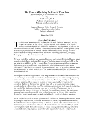
  • 3. Overview of the Puzzle ur team at the University of Louisville was engaged over the summer by the Louisville Water Company to study the causes of recent decline in residential water use per customer. Residential water usage per customer has fallen as the number of residents and households continues to grow, and as household incomes continue to rise. The chart below summarizes thirty years of monthly data on average water usage per residential customer. A 12-month moving average was constructed to smooth out variations in month- to-month use due to seasonal demand and billing anomalies. It is clear that water use per customer has fallen significantly. Water usage peaked in late 1988 at around 7,000 gallons per month. Today, the average customer uses only 5,600 gallons per month, a decline of 20 percent from the peak. This has serious revenue implications for the Louisville Water Company. Stable revenues are needed to finance the capital programs required for replacing legacy water mains and extending water service to new suburban communities. Increased water rates are the most direct way to recoup revenues from falling water usage, but if the Company continues to raise water rates there will eventually be resistance from homeowners and voters. It has become increasingly urgent to understand what is causing the decline in residential water sales. O Water Usage per Residential Customer gallons by month, 1975-2004 4,000 5,000 6,000 7,000 8,000 9,000 10,000 11,000 Jun-75 Jun-76 Jun-77 Jun-78 Jun-79 Jun-80 Jun-81 Jun-82 Jun-83 Jun-84 Jun-85 Jun-86 Jun-87 Jun-88 Jun-89 Jun-90 Jun-91 Jun-92 Jun-93 Jun-94 Jun-95 Jun-96 Jun-97 Jun-98 Jun-99 Jun-00 Jun-01 Jun-02 Jun-03 Jun-04 12-month centered moving average Several hypotheses have been advanced to explain the reduction in residential water usage. 1. Wetter weather has reduced the need for outdoor watering. There is a clear negative relationship overall between rainfall and water usage per customer. The peak water usage period (1988) in the chart above was among the driest in thirty years. The relationship between average residential water usage and ground moisture is clear in the chart below. We focus here only on the April to September months, when outdoor watering of lawns and landscaping is most prevalent. The Palmer Drought Residential Water Sales, Louisville Water Company 3
  • 4. Severity Index provides a general measure of ground moisture for the central Kentucky region. One can easily see the negative relationship between ground moisture and residential water usage. The driest years, 1986 and 1988, were the ones with the highest water usage. The wettest years, including the last two years, have low water usage. We investigate this more carefully with an econometric model presented later in this report. 2. The average number of persons per household has been falling, thereby reducing the total water usage of the typical household. It is certainly true that the number of persons per household has been falling in Jefferson County. The last four decennial censuses revealed a decline from 3.16 persons per household in 1970, to 2.69 in 1980, to 2.48 in 1990, and to 2.37 in 2000. This represents a twenty-five percent reduction in household size in just three decades. Industry research shows that water usage is indeed sensitive to household size, as less people means less laundry, less dishwashing, less bathing, and less toilet use per household. Our econometric work, as well as the research of others, suggests that an additional person in a household leads to between 600 and 1,100 gallons more water usage per month (depending on age). Played in reverse and applied to the local situation, a drop in average household size in Jefferson County from 2.92 to 2.35 persons during the 1975 to 2004 period, would lead to a decline in monthly water usage of between 340 to 630 gallons per residential customer. This range nicely brackets the actual net decline in average usage (525 gallons per month per customer) seen by the Louisville Water Company over the period. However, note from the first chart above that all of the decline in water usage per customer has occurred since 1985, while household size has been falling for decades. So, while falling household size has no doubt contributed greatly to declining water sales, it is evidently not the only causal factor. Something else was Average Residential Water Use vs. Ground Moisture Index April to September, 1975 - 2004 30,000 35,000 40,000 45,000 50,000 -5 -4 -3 -2 -1 0 1 2 3 4 5 Palmer Drought Severity Index (-5 severe drought, +5 saturated), April to September only AverageResidentialWaterUsage 2000 1999 1988 2004 1975 2003 1989 1986 1979 Residential Water Sales, Louisville Water Company 4
  • 5. causing water usage per customer to rise in the earlier period even as there were fewer people per household each year. 3. Federal water-conservation laws have required manufacturers to make water appliances that use much less water, beginning in the mid-1990s. Most major plumbing ware manufacturers began in 1994 to produce low-volume toilets, urinals, showerheads, and faucets that comply with the Energy Policy Act of 1992 regulations1 . Thus, contractors have been installing low-flow water appliances in new homes and in renovation projects for a decade now. These new appliances use on net less than half the water per use as older appliances, though it is unclear how much of this decline is offset by longer showers, multiple flushes, and second rinses in the clothes washer. The Louisville area has seen a surge in home construction, and Jefferson County has added 50,000 new housing units since 1990, accounting for over one-sixth of the current housing stock. The chart below shows the distribution of new housing (authorized) among single-family and multi-family units. Declining interest rates have particularly spurred single-family home construction since the early 1990s. An end use modeling system would be required to understand the importance of the new water-conserving appliances on water usage by household. Data loggers would need to be installed on water meters in a sample of homes, with profiles developed on the physical characteristics of the home and the demographic and economic characteristics of the people living in the home. By controlling for these many factors, analysts could determine the incremental effects of low-flow toilets, showers, dishwashers, and clothes washers on the household’s water usage. Housing Units Authorized, Single and Multi-Family Jefferson County, Kentucky 1,694 1,669 1,590 1,684 1,869 2,266 2,714 2,799 2,480 2,567 2,508 3,087 3,027 2,797 2,978 2,749 3,164 3,237 1,681 1,120 738 762 537 637 343 855 627 871 480 1,026 1,323 1,012 599 761 831 649 0 500 1,000 1,500 2,000 2,500 3,000 3,500 4,000 4,500 5,000 1987 1988 1989 1990 1991 1992 1993 1994 1995 1996 1997 1998 1999 2000 2001 2002 2003 2004 Source: US Census Bureau. Multi-Family Units Single-Family Units 1 Source: letter from Amy Vickers and Associates to CH2M Hill Engineering, September 20, 1994. Residential Water Sales, Louisville Water Company 5
  • 6. Without an end-use study, we have only aggregate data on which to base estimates of the effects of the new water-conserving appliances. In the econometric work presented later, we develop a proxy for the introduction of water-conserving appliances in the mid-1990s. Basically, we assume that all new homes are equipped with lower-flow appliances and measure their rising share of the County’s total housing stock. This measure, while admittedly crude, is statistically significant in one model developed to explain the reduction in average water use among residential customers. 4. A large proportion of households are classified as commercial water users in the Water Company’s database. These households include apartment dwellers and condo owners. We have extensively investigated this classification issue, using a random sample of 500 Louisville Water Company ‘commercial’ customers in 2004. We found that the sample included 162 residential premises, containing 1,528 housing units. The sample results were adjusted for occupancy and applied to a County-wide estimate, suggesting there are 44,200 occupied housing units in the County counted under the commercial customer classification. This represents about one-sixth of all occupied housing units (of any type) in Jefferson County. A detailed discussion of our investigation is provided later in this report. It is revealing to examine the growth in residential water customers and housing units in Jefferson County between the last two decennial censuses. There is a tight fit between the net growth in residential water customers and occupied housing units in the County. Between 1990 and 2000, the Water Company gained 26,400 customers classified as residential (from 193,400 to 220,800 customers). The Census Bureau reports a growth of 23,800 occupied housing units over the decade (from 264,200 to New Housing vs. Growth in Residential Water Customers 0 1,000 2,000 3,000 4,000 5,000 6,000 1988 1989 1990 1991 1992 1993 1994 1995 1996 1997 1998 1999 2000 2001 2002 2003 2004 Annual growth in residential water customers, December to December New housing units authorized in Jefferson County, single and multi-family 287,000 units). The Census figure includes both owner-occupied and renter-occupied Residential Water Sales, Louisville Water Company 6
  • 7. housing units (186,400 and 100,600 respectively in 2000), but the Census does not provide a breakout for single-family versus multi-family. Annual building permit data follow the same general pattern as new residential ere e ote that if one adds the number of average residential water customers (237,800) in he y ounting apartment units as commercial customers causes a reduction in measured er of uilding permit records indicate that there are on average about 700 multi-family l ther water utilities around the United States are also now facing a decline in residential ts of , water’s low price, and modest population growth. customers, though the cumulative numbers do not align2 . The data show that th were 25,000 new single-family homes authorized over the decade, plus 7,500 new multi-family units. So, it appears that about 6,000 more units were built than can b accounted for by the net growth in residential customers or occupied units. Much of this discrepancy is due to demolitions, particularly around the airport and in older neighborhoods west of Interstate 65. N the year 2004 to our estimate of occupied housing units classified as commercial customers (44,200), you arrive at 282,000, only three percent less than the Census Bureau’s estimate of the number of households (292,300) in Jefferson County for t same year. The difference could be due to a higher occupancy rate for apartment units than we assumed (90 percent), to sampling error, or to other Water Compan classification issues. C residential customers, but also a biased measure of water usage per residential customer – at least in the literal sense of the word residential. The average numb persons living in a rental unit is less than in an owner-occupied dwelling. The 2000 Census reports 2.14 persons per rental unit versus 2.50 persons per owner-occupied unit in Jefferson County. Given that fewer persons per unit translates directly into lower water use per unit, we can infer that if all the multi-family housing units were counted as residential customers, residential usage per customer across the system would be even lower than now perceived. B units (apartments or condominiums) built in Jefferson County each year. Nearly al of these households continue to be classified as commercial customers. The mixing of households between the residential and commercial classifications makes an analysis of household water usage more difficult. O water use per customer, and industry analysts are beginning to focus on the causes. However, as will become evident in the next section, the literature on the determinan household water usage is not very mature. Estimates vary widely of the effect of changing household size, of conservation laws, and of the response to price and income increases. Moreover, most of the relevant research has focused on water usage in the arid Southwest where water rationing is a common occurrence. The paucity of research on household water usage in the Midwest is no doubt due to the region’s historically ubiquitous water supply, 2 The three spikes in the chart showing growth of residential water customers are due to the conversion of wholesale customers into residential customers – Jeffersontown (1990), Bullitt Kentucky Turnpike #2 (2000), and Goshen and Shepherdsville in 2002-03. Residential Water Sales, Louisville Water Company 7
  • 8. Review of Industry and Academic Research on Residential Water Usage Modeling n this section, we provide a summary of the published literature on residential water usage. We have scoured industry and academic sources to identify any studies that have looked at the issue of fluctuating water demand, with particular emphasis on quantifying the factors that cause households to consume more or less water over time. The literature provides some studies that help us understand what is causing the decline in average residential water use in Louisville. Many variables have been used to fit demand models over the last century, including water price, household income, outdoor water use, weather, and household size. The dissemination of low-flow water appliances, prompted by the Energy Policy Act of 1992, has spurred a fresh literature that focuses on water technology as a variable also. A complete list of the studies cited is provided in a reference section at the end of this report. There are two basic methods used to analyze household water usage, econometric and end- use. Econometric models have been fit using historical data on aggregate residential water use for a system or for usage by individual households at a point in time or across time. Residential water usage per customer by month is modeled as a function of weather, water price, household demographics, technology, and other economic-demographic factors. These models are also essentially models of shifting demand. Water supply is taken to be inelastic at the given water price, regardless of quantity consumed. The quantity of water demanded by a household may be price-sensitive at very high prices per gallon, but is quite inelastic over the range of prices seen historically in the Midwest. That is, a rise in water price of ten to twenty percent would not cause residences to use much less water. And a similar drop in water prices would not cause residences to use much more water. The actual water demand, and hence usage, in a market is determined by how weather and other factors shift the demand curve, not by water prices. The textbook supply and demand diagram above is useful as a conceptual starting point only. The market for water is more complex, particularly when considering changes over time. As with gasoline, electricity, medicine, and other necessities of life, demand for water I gallons of water per month $15 6,000 Price per thousand gallons Supply Demand Residential Water Sales, Louisville Water Company 8
  • 9. will certainly be more price-sensitive once consumers have a period to adjust. In the short- onths), consum their housing r term (m characteristics and lifestyles cannot be changed immediately. But over several years, people would respond to higher water rates by installing more efficient appliances, fixing leaky fixtures, and reducing outdoor watering. Moreover, the supply curve is not fixed over time. The technology of water delivery is always improving, putting downward pressure on price. The flatness of the supply curve is only an approximation around the point of typical wate usage. There are great economies of scale in water production and distribution, so that costs (and therefore prices) fall dramatically as customers are added, particularly in a densely populated area. ers have little choice but to pay higher rates, as End-use models are inherently micro. They focus on the water usage of individual households. A housing unit is characterized by its physical and plumbing features, including hether therew is outdoor water usage for a garden, landscaping, or a swimming pool. The household is characterized by demographic features such as number of residents and their ages, and by economic factors such as the number of working members of the household and their incomes. Special water metering devices are installed, or diaries are kept by someone in the household, to monitor water usage by day or even time of day. Statistical analysis is performed after sufficient data are acquired, to determine the differential impacts of housing and household characteristics on water usage. The most comprehensive end-use modeling reference is Residential End Uses of Water, by Mayer et al. (1999). This study was sponsored by the American Water Works Association Research Foundation. The investigators randomly selected 1,000 households from billing records in each of fourteen cities in North America, then chose a sub-sample of 100 in each for detailed data-logging. While most of the cities were in the western US, two were in Ontario and are presumably more like Louisville in terms of water availability and usage. The study reports detailed distributions and statistics on water usage in each city, including per capita daily usage for toilets, showers, baths, faucets, clothes washers, dish washers, leakages, and other indoor uses, as well as measurements of outdoor usages. We summarize the relevant findings from the major end-use and econometric studies below, organized by the key variables thought to determine household water use. Household Demographics The literature points to a positive relation between residential water demand and number of members of a household. Moreover, researchers have suggested that a change in number of people in a household causes a less than proportional change in water demanded (Howe and Linaweaver, 1967). There are economies of scale in water usage for a household, particularly for dishwashing and laundry, so that water use is not expected to be a linear function of the number of persons per household. In a recent study conducted in Spain, the elasticity of water usage with respect to family members was between 0.734 and 0.868 (Arbues and Barberan, 2004). Older estimates place the elasticity between 0.25 and 0.74 (Morgan 1973, Grimm 1972, Danielson 1979). These studies implicitly assume a constant elasticity, and hence a hyperbolic relationship between number of residents and household water use. Residential Water Sales, Louisville Water Company 9
  • 10. For studies fitting a linear relation between indoor water use and size of the household the elasticity is not constant. Mayer et al. (1999) use a large pooled sample of individual households to find a linear relationship as follows: (indoor water use per day) = 69.2 + 37.2 (number of people per household). So, if the average number of persons per household were to fall by, say, 0.5, then using this equation we would expect the average household water consumption to fall by 558 gallons per month. This represents a significant reduction from a typical base water usage of 6-7,000 gallons per month. Other research suggests that the age composition of a household is a statistically signific determinant of w ant ater usages (Lyman 1992, Hanke and de Mare 1982). Lyman finds that another child would increase water usage in a home by about 2.5 times that of another“ teenager and 1.4 times that of another adult”. Price Elasticity There are no substitutes for water in its basic household uses, and hence economic theory predicts that residential consumption will be very inelastic with respect to price. Moreover, water prices have historically been low enough that water bills typically account for a percentage of a household’s monthly income. Thus, consumers are often not even aware when water prices change and this makes it even less likely that consumption would change in the face of small price variations. However, there are goo small d a priori reasons to believe the rice elasticity of water is not zero. Beyond drinking and sanitation uses of water, much , s ld eek nge in water usage allons) divided by the percentage change in water price per gallon. We say that water is usehold goes own five percent we say that the price elasticity of demand is -0.5, or inelastic. It is the price elasticity of demand can change dramatically over the cases, however, but on the effect of price changes in the eighborhood of typical water rates and monthly usages. dy ointed to price elasticities of demand of round 0.5 (Gottlieb 1963). Howe and Linaweaver (1967) found the price elasticity to be p household water usage can not be deemed a necessity. Sprinkler systems for landscaping garden irrigating, car washing, and swimming pool refilling would all likely see reductions a water prices rose appreciably. Leaky plumbing that might be ignored under low prices wou be repaired under high prices. And even some sanitary uses would be curtailed under very high prices, as many people would find that they get along fine with four showers per w instead of eight to ten. Finally, as is evident from these examples, households’ response to higher water rates will be much greater over several years than several weeks. The price elasticity of water demand is defined as the percentage cha (g price elastic if the ratio is greater than one in absolute value, and inelastic if it is less than one. So, if water price per gallon goes up ten percent and water usage per ho d important to recognize that theoretical range of prices. For example, in the extreme case of very expensive water households will continue to purchase enough water to survive, and thus demand is very inelastic for further price increases. Similarly, at the other extreme, water that is approaching a zero price per gallon will not cause the typical household to consume much more water than before. The price elasticity of water is inelastic to price decreases in this case. Most analyses focus not on these extreme n There is a long literature on the sensitivity of residential water demand to changes in water prices. A 1926 article in the Journal of the American Water Works Association reported on a stu of 29 utilities, and indicated a definite reduction in water use per residence as price rose (Metcalf 1926). Studies in the 1905s and 1960s p a Residential Water Sales, Louisville Water Company 10
  • 11. about -0.4, but pointed out that this sensitivity is composed of an indoor water usage elasticity of -0.2 and a ‘sprinkler’ or outdoor water usage of -1.6 for humid eastern ar as Louisville. That is, indoor water usage was found to be relatively insensitive to price, but outdoor water usage to be Espey, Espey, and Shaw (1997) preformed a meta-analysis on 30 years of research in the field of price elasticity of water. Their research concluded that eas such the average price elasticity of ater for residential use was -0.51 with 90% of the estimated elasticities falling between 0 spiration influenced the price elasticity stimate. A number of variables that were found to be important to determining total water appear to effect price elasticity, including temperature, household size, and w and -0.75. The literature includes studies with very different model specifications and estimation methods, and the focus of this paper was to investigate how the ultimate price elasticity estimates in the literature were affected by model and variable choice. Including variables such as income, rainfall, and evapotran e demand did not population density. Also, price elasticity estimates were not sensitive to whether the models were fitted with cross sectional or time series data, or with aggregated or disaggregated data. Another review article, by Arbues et al. (2003), also finds a range of price elasticity estimates. These authors examine three types of model specifications over fifty papers. The estimates range generally between -0.1 and -0.7. Like Espey et al., the findings reviewed have a midpoint elasticity estimate of around -0.5. Income Elasticity The sensitivity of water usage with respect to household income has also been analyzed through a variety of lenses, and the empirical results vary widely. At the individual household level it is usually not feasible to obtain direct measurements of income. “Assessed value of the property,” first used by Howe and Linaweaver (1967), is a common surrogate for household income. Real estate values are public information, easily obtainable for each ddress, and are known to be highly correlated with income. Other proxies for income in the of , se in e e utdoor Use a literature include the education level of the household head, age of the home, occupation household head, and number of cars (Jones and Morris 1984). Howe and Linaweaver (1967) report an income elasticity of 0.35 for residential water usage implying that a 10 percent increase in household income leads to a 3.5 percent increa water usage. In the review article by Arbues et al. (2003), income elasticities are reported between 0.15 and 7.83, a vast range. The problem for these and other researchers is to separate the income effect from all the other income-related effects. As household incom rises, we see fewer persons per household, but more outdoor water uses (irrigated landscaping, swimming pools). Moreover, the typical water bill is a very small fraction of th income of affluent people, suggesting lower price elasticity than for poorer households (though this was not found in the meta-study of Espey et al., 1997). O Research focused on time of year suggests that summer water demand is more elastic than winter water demand (Arbues et al. 2003, Mayer et al.1999, Howe and Linaweaver 1967). Originally winter demand was considered non-seasonal demand, while the difference between summer demand and winter demand was categorized as seasonal demand (Howe and Linaweaver 1967); but more recent research, with access to disaggregated end-use Residential Water Sales, Louisville Water Company 11
  • 12. analysis, suggests that indoor water usage also fluctuates with the time of the year and that outdoor water use also occurs in the winter (Mayer et al. 1999). They have shown that outdoor use rises in concert with the square footage of the home and lot size. They theorize that both exogenous variabl thus es serve as indicators of standard of living. Also, the outdoor ater price elasticity, which they calculated as -0.82, is relatively elastic compared to overall se homes which water with a hand-held hose use 33% less water outdoors than other tility, water source displayed 25% less outdoor use than those without access w water price elasticity, in accord with economic theory. Other findings of outdoor water u in their detailed end-use study include: homes with swimming pools use more than twice as much water outdoors than homes without them homes with in-ground sprinkler systems use 35% more water outdoors than those who do not homes that use an automatic timer to control their irrigation systems used 47% more water outdoors than those that do not homes with drip irrigation systems use 16% more water outdoors than those without them homes homes which maintain a garden use 30% more water outdoors than those without a garden homes with access to another, non-u Weather Weather has been shown to affect seasonal water demand, though results vary geographi and it is difficult to generalize. Nieswiadomy (1989) investigated the interaction of w and price elasticities, calculating the difference between potential evapotranspiration for Bermuda grass and actual rainfall. Evaportranspiration was shown to significantly alter the own-price elasticity of water. Others have used precipitation during the growing season, minutes of sunshine, and annual rainfall (Arbues et al. 2003). As measured by Miaou (1990), weather was shown to be hystere cally eather tic, dynamic, and state- ependent: hysteretic, the response to temperature at different temperatures is different at all. d different times of the year; dynamic, rainfall’s effect diminishes over time; and state- dependent, the higher seasonal water use before rain “the more water use reduction can be expected.” Weather is thought to have non-linear effects on water usage. According to Miaou’s statistical analysis the number of rainy days is a better predictor than total rainf Technology and Regulation A literature is emerging on the effects of household water technology on indoor water usage (White 2004). Most research in this area has focused on conservation, induced by the Energy Policy Act of 1992 and its regulations on plumbing-ware manufacturers. In one tudy the introduction of low-flow water technology reduced water consumption per 6%, in another 46% (Mayer et al. 2003, Mayer et al. 2004). With such s household by 3 significant drops in usage reported in the literature, it seems likely that the introduction of water-conserving appliances has contributed to the drop in per customer usage in the Louisville area. However, as far as we know, no Louisville-specific research has been performed to determine the saturation of these appliances in the local housing stock. Residential Water Sales, Louisville Water Company 12
  • 13. Customer Classification Issues ouisville Water Company officials are well aware that many customers classified as ‘commercial’ are in fact households, not business establishments. However, until this study the extent of the classification problem was not known. This section addresse issues of residential and commercial customer classification in the LWC database. We examined a random sample of 500 commercial customers and found that the sample contained 162 premises with 1,528 hous s ing units. These units were primarily apartment com ified as comm r sample results imply that about 15 percent of all housing unit custom Company database. Interestingly, the average commercially classified hou g We begin with a brief discussion of common approaches to customer classification within the u customer database. We then provide a statistical characterization of the entire Company data s appro c we identified commercial customers that actually represented housing units, and w Cla f The water industry does not have a stan ic research and industry officials acknowledge that to water usage data when o and irrigation services. In the delivery of potable water, typically es s or L plexes and condominiums, though we did discover several single-family homes class ercial customers. Ou s in Jefferson County are counted under the commercial, rather than residential, er class in the sin unit uses more water than the average residentially classified housing unit. ind stry, and explain the classification system used in the Louisville Water Company ba e, showing the distribution of customers by type. Finally, we describe the sampling a h, how ho inferences were made county-wide. ssi ication Methods within the Industry dardized methodology for customer billing ions. However, both academclassificat most water companies group customers according to similar ‘use characteristics’ such as amount of water consumed, topographic constraints and service type, rather than actual property use (Dziegielewski et al. 2002)3 . This approach to customer classification poses a problem in trying to understand water consumption patterns based on economic and demographic models. For example, economists analyze water demand and supply in the same way they analyze other goods and services. They use consumer theory to model ousehold water demand. But it is difficult to apply these modelsh household water use is measured under a commercial classification because a business happens to own a multi-family housing complex. In practice, customer classes are influenced by service type. Service types are distinguished first by whether the water is for potable or non-potable use. Potable water is defined as water suitable for drinking, cooking and irrigating on a domestic scale. Non-potable water refers t ater used for large area irrigation, fire, and industry. Both residential and commercialw customers use potable water customers are grouped into one of two broad categories, residential and nonresidential users. These categories are further divided into subsectors that vary among water companies. For example, some water companies treat all single family, multi-family units and mobile hom as residential, while other companies may categorize apartment complexes, mobile home 3 The statement is also based on phone conversations with officials at the Kentucky Public Service Commission and the Louisville Water Company. Residential Water Sales, Louisville Water Company 13
  • 14. condom busines Custom The Lo iniums as commercial. This is particularly true if the account is registered to a of rvices ater Large Domestic Services s that d r s rather than an individual person (Dziegielewski et al. 2000).4 er Classifications within the Louisville Water Company uisville Water Company identifies seven customer billing classes: Residential, Commercial, Industrial, Fire Hydrant, Fire Service, Municipal and Wholesale5 . Types services offered by the Water Company include Domestic, Fire, Irrigation, Combined Residential Domestic/Fire and Combined Commercial Domestic/Fire6 . The scope of this study includes only LWC customers who received domestic water se in 2004. The table below refers to the categories of domestic service available to Residential and Commercial customers as defined in the Louisville Water Company Board of W Works Rules and Regulations. The meter sizes typically used in each category are taken from the distributions found in our analysis of the 2004 customer billing data. Residential and Commercial Billing Classes Under the Louisville Water Company’s Domestic Water Services LWC DOMESTIC W Single Family Residential A single family house typically uses a ¾" domestic service for water usage. Larger size meters are available. Domestic service are larger than 4". The customer provides the point of highest flow an the point of lowest flow for meters over 2", so that the optimum mete assembly can be constructed to best serve that location. Water Irrigation Irrigation Water Meter sizes typically range from 5/8” to 4” Meter sizes typically range from 5/8” to 3” Meter sizes typically range from 5/8” to 6” Meter sizes typically range from 5/8” to 8” Includes two or fewer housing units, residential properties held in common such as condos and non-residential farms. establishments engaged in selling merchandise or rending service, construction, mining, agriculture, and condominium units owned by developer. Residential Commercial A separate meter placed at a location to be used specifically for irrigation systems on the site. The irrigation meter counts the water separately and will save the customer the MSD sewer charges in areas that are served by MSD. ATER SERVICES Includes non-manufacturing industries, tionIrriga 4 See also online references: Local Water Utilities Administration, 2005; and City of Salem Finance Department, 2005. 5 LWC online < http://www.lwcky.com/water_works/default.asp> 2005. Louisville Water Company Board of Water Works. Rates, sec.6.01 through 6.09. ice . 6 LWC online < http://www.lwcky.com/water_works/default.asp > Service Applications/ 2005 Serv Rules and Regulations, Sec. 1.04.1 through 1.04.5 Residential Water Sales, Louisville Water Company 14
  • 15. Characteristics of the LWC Customer Database This section highlights the structure and characteristics of the billing data. The customer billing data provided by LWC for analysis included 1,486,098 individual records that throughout Jefferson, e days le below provides brief explanation of each field in the database. This is followed by a more detailed represented every bill issued to commercial and residential customers Bullitt and Oldham counties in 2004. Billing information contained within the databas included premise number, attachment number, account name, service address, service zip code, mailing zip code, customer type, service type, meter size7 , billing date, number of billed, and volume of water used during each billing period cycle. The tab a explanation of various aspects of the billing information and their distributions. Customer Record Fields Used in Study Field Label Definition PREMNUM Premise number s where water meter (or meters) is attached. Each physical address has only ay have multiple meters. Specific number assigned to physical addres one premise number, although it m ATTNUM Attachment number ise may have more e meter, therefore more than one attachment number connected to the premise number. However, a meter has only one attachment number. This is the only unique ID field in the database. Specific number assigned to each meter. A prem than on ACCTNAME Account name Name of the business or individual(s) responsible for payment on the account. SERVADD Service address Physical address of the premise. SERVSIZE Service size Size of water meter of given attachment number. SERVTYPE Service Type Type of service, either Water or Irrigation, to given attachment number. TAXDIST Tax District Tax District where premise is located. RESCOMM Residential or Commercial Type of customer, either Residential of Commercial, never both. PREMZIP Premise zip code Zip code of premise address. ACCNTZIP Account name zip code Zip code of address of person(s) or business in whose name the account resides. BILLDATE Date of bill Date by month, day, and year the water bill was issued. BILLDAYS Number of days billed Number of days in the billing cycle for which the premise was billed. USAGE Water use in billing period (000s gallons ) Amount of water used in the billing cycle, measured in one- thousand gallon increments. 7 Meter sizes were not available for 6,925 meters in Bullitt and Oldham counties. Residential Water Sales, Louisville Water Company 15
  • 16. Premise and Attachment Numbers The LWC customer billing data is based on premise numbers and attachment numbers. Each physical property with a meter issued by LWC has a premise number. In effect, premise number is connected to the site address. There is only one premise number for every address, although a premise may have more than one meter. For example, there m be two or more meters of different sizes, or one or more meters measuring potable water and one or more measuring irrigation. Each meter on a premise is assigned a unique attachment number. Premise and attachment numbers remain a permanent record feature connected to specific physical addresses, even though the account name assigned to a address may change. For example, a rental property may change account names tw the ay n o or more mes in a given year, yet the premise number assigned to that address and the attachment number or numbers assi is is true for every premise, resid r commercia d or owned. M ti 3/4" 7,799 Other 241 3% 61 3% 1% 2" 389 0% 4" 187 0% 6" 43 0% 8" 10 0% 10" 1 0% 0% 108,593 1" 6,7 11/2" 1,940 1,708 1% 3"5/8" X 3/4" 5/8" 124,800 49% 43% gned to the premise remain the same. Th ential o l, rente eters All water supplied by the Louisville Wate measured by meters installed and maintai The Water Com e amou water a premise uses over one or two-mo billing cycles as indicated by the on-prem m ter rying sizes in diameter, anywhere from 5/8” to 5/8” X 3/4” (a low/high-flow feature) to 10” depending on the volume of w i anuf stomer whose production process depends o ume ally have meters of at least 4” in diameter and more likely 6” to 8” diameters while a ily re would n e 5/8 3/4” to 3/4” meters. Customers in the LWC r Company is ned by LWC. nt of nth pany calculates th ise eters. A me can be of va ater needed by the customer. An ndustrial m acturing cu n large vol s of water would typic single-fam sidential customer ormally us ”, 5/8” X Residential and Commercial Three-County Service Area Residential Water Sales, Louisville Water Company 16
  • 17. Customer Classes and Service Types Irrigation 5,425 2% Commercial premises 21,009 8% Potable Water 253,681 98% LWC identifies seven customer classes including residential, commercial, industrial, fire service, fire hydrants, municipal, and wholesale. The two customer classes included in this analysis are residential and commercial. And while there are a number of service type classifications within the LWC billing structure, this analysis includes only two, potable wate and irrigation, both of which fall under the broader category of domestic service provided the Company. Broken out by premises, the residential class accounts for 92% of LWC’s commercial d residential r by , an customers and delivery of potable water Residential premises 238,118comprises 98% 92% of overall demand in the three county area. Meter Size by Customer Class8 Although smaller meters are the norm in e si the 10" 1 0% 6" 43 0% 4" 186 1% 8" 10 0% no meter size given 427 2% 3" 385 2% 2" 1,635 8% 95 3/4" 1,203 6% 5/8" 5,521 25% 531 1 1/2" 1,7 9% 1" 4, 22% 5/8" X 3/4" 5,272 25% 3/4" 6,596 3% 4" 1 0% 2,230 1% no meter s e given 6,448 3% 0% 119,279 50% 43% 1" 0% 73 0% 3" 4 iz 1 1/2" 145 2" 5/8" 5/8" X 3/4" 103,321 ze of ercial ial Class The pie chart at left shows the predominance of smaller meters in use among customers classified as residential. delivery of water for domestic use, th ommmeter varies, particularly among C customers. This variation was a flag in looking for residential properties classified as commercial. The figure to the right depicts the variance in meter sizes used for water delivery to commercial customers in the LWC service area. Meter Size by Residential Class Meter Size by Commerc 6,925 meters among 6, 875 premises in Bullitt and Oldham counties lacked identification by meter size.8 Residential Water Sales, Louisville Water Company 17
  • 18. Meter Size by Service Type Meter sizes vary according to service type as well as customer class. Although there is a g deal of overlap, this analysis found that surprisingly, the larger meters were used more among customers of potable water service than of irrigation services. However, as the c below indicate, the typical meter size applied to the delivery of irrigation services was generally larger than the 5/8” or 5/8 X 3/4” meters that dominate in delivery of potable water. Residential Water Sales, Louisville Water Company 18 1" 6,053 2% 1 1/2" 1,789 1% 2" 1,538 1% 3" 382 0% no meter size given 6,842 3% Other 6,894 3% 6" 41 0% 8" 10 0% 10" 1 0% 4" 185 5/8" X 3/4" 107,505 42% " 67 5/8" 124,768 49% 0% 3/4 4,5 2% 3" 732 1% 2" 170 3% 1 1/2" 151 3% Other 44 no meter size given 33 1% /8" X 3/4" 20% 59% 1" 13% 0% 4" 2 6" 0% 2 0% 5/8" 3/4" 3,232 1% 1,088 708 5 reat harts Meters ater Distribu b For Distribution of by Size For Potable W tion of Meters y Size Irrigation
  • 19. Random Sample of Commercial Customers This section describes our analysis of a random sample of 500 commercial customers within Jefferson County. Our objective in pulling a sample was to learn how many properties classified as commercial were actually in residential use. Here we explain how the random sample was obtained and the property use identified. This is followed by a discussion o distribution of customer characteristics and water use within the sample. The results of th sample f the e analysis are then used to construct estimates of the total number of housing units overed by the commercial class of customers within the County. m Sample c Criteria for the Rando The random sample . The crite was pulled from a universe of 16,074 premises classified as commercial ria for forming the universe of commercial customers from which to tract the sample were the following: each customer (premise) should have one year of ontinuous service to at least one meter on premise in 2004; use either [domestic] water or irrigation services; be classified commercial and be located within Jefferson County. he number of bills received in 2004 served as a proxy for one full year of service. Any tachment number that received 6 or more bills in 2004 qualified. Using SPSS 13.0, the umber of residential and commercial customers in Jefferson County was derived by ducing the original database of 1,486,098 billing records in the three-county area to only ose records whose Tax District was listed as Jefferson County. Next, we identified records ith Service Types of either Potable Water (W) or Irrigation (I), dropping all others. Finally, e identified how many bills went to each meter in 2004, and within that pool, how many remises had meters with six or more bills sent in the course of the year. fferson County Residential and Commercial Customers customers ex c T at n re th w w p Je Residential Water Sales, Louisville Water Company 19 Residential 185,027 92% Commercial 16,074 8% he number of residential and commercial premises with a continuous year of water service Jefferson County totaled 201,101, with a distribution of 92% residential customers and me proportion found in the overall data for the three counties. ccounted for 99.9% of the delivery service type, a slightly higher proportion rea. T in 8% commercial, the sa Potable water a than in the larger a POTABLE WATER 200,828 99.9% IRRIGATION 273 0.1%
  • 20. Meter Sizes by Service Type The following two charts illustrate the distribution of meters by size and service type for those residential and commercial customers in Jefferson County who received at least six during the course of the year. The first pie chart represents the distribution of meters used the delivery of Potable Water Service and the second chart illustrates the distribution as it applies to Irrigation Services. Jefferson County Commercial and Residential C 1 1/2" 23 8% Other 42 15% 4" 1 0% 3" 1 0% 2" 40 15% 5/8" 3 1% 4" 0 % 1" 60 %5/8" X 3/4" 45 16% 3/ 10 38 22 8" 6 6" 16 0% 4" 127 0% Other 149 0% 3" 301 0% 3/4" 3,852 2% 5/8", 102,061, 50% 5/8" X 3/4", 85,999, 43% 0% 1% 2" 1,417 1 1/2" 1,627 1% 1" 5,422 3% bills in ustomers 1 Year of Service for Potable Water istribution by Meter Size in 2004D Jefferson County Commercial and Residential Customers 1 Year of Service for Irrigation Distribution by Meter Size in 2004 Residential Water Sales, Louisville Water Company 20
  • 21. Potable W 15,95 99 ater 1 % Irrigation 123 1% 4" 2 5/8" 12 0% 3" 11 2% 2" 42 9% 1 1/2" 48 10% 16 % 5/8" X 3/4" 131 27% 3/4" 21 4% 3 %25 1" 1 23 2" 2 33% 1 1/2" 4 67% Potable Water 494 99% Irrigation 6 1% sample was pulled from only Commercial customers in ate Pota Among Jefferson County Comme with One Full Year of Servic Proportion of Potable Water and Irrigation Services Among the Random Sample Distribution of the Random Sample by Meter Size for Potable Water Service Distribution of the Random Sample by Meter Size for Irrigation Service As previously stated, a random Jefferson County, a universe of 16,074 premises. The two charts immediately below illustr the proportion of customers using Potable Water and Irrigation Services among the universe of Jefferson County Commercial premises and the random sample respectively. These are followed by two charts that represent distributions of the random sample broken out by Service Type and Meter Size. Proportion of ble Water and Irrigation Services rcial Premises e Residential Water Sales, Louisville Water Company 21
  • 22. The map below shows the spatial distribution of the random sample overlaid on Jefferson County land use zones. Residential Water Sales, Louisville Water Company 22 #* #* #* #* #*#* #*#* #*#*#* #* #*#*#* #* #*#* #* #* #*#* #* #*#* #*#* #* #* #* #*#* #*#* #* #*#* #*#* #*#* #*#*#* #* #*#*#*#*#* #* #*#* #*#* #* #*#* #* #* #*#* #* #* #*#* #*#* #*#*#* #*#* #* #*#*#*#*#* #* #*#* #*#* #*#* #*#* #* #* #* #*#*#* #* #*#*#* #* #* #* #* #*#* #* #*#* #*#*#* #*#* #* #* #* #* #* #* #* #* #*#* #*#* #* #*#* #*#* #*#* #*#*#* #*#* #*#* #*#*#* #* #* #* #* #* #* #* #* #* #* #* #* #*#* #*#*#* #* #* #* #*#*#* #*#* #* #* #*#*#* #* #* #*#*#*#* #* #*#* #*#*#* #*#*#*#*#* #* #* #*#* #* #* #* #* #* #* #* #* #* #*#* #* #* #* #* #* #*#*#*#* #* #* #* #* #* #*#*#* #* #* #*#* #* #*#* #*#* #*#*#*#* #* #* #* #* #* #* #* #*#* #* #* #*#* #* #* #* #* #*#* #* #*#* #*#*#*#* #* #* #* #* #* #* #* #* #*#* #* #* #* #*#* #* #* #*#* #* #* #* #* #* #* #* #* #*#* #* #* #* #* #* #* #* #* #* #* #*#* #* #*#* #* #* #* #*#* #* #* #* #* #* #*#*#*#* #* #*#* #*#* #* #*#*#*#*#* #* #*#*#*#* #*#* #*#* #*#*#* #* #*#*#*#* #*#*#* #* #*#* #*#*#*#*#* #* #* #*#* #* #* #* #*#* #*#*#*#*#* #* #* #* #* #*#* #*#* #* #*#*#* #*#*#* #*#* #*#*#*#* #* #* #*#*#*#* #* #* #* #*#*#*#*#*#* #* #*#* #* #*#* #* #*#*#* #* #*#* #*#* #*#*#* #* #*#* #* #*#* #* #* #* #* #*#*#* #*#* #* #*#* #* #*#* #*#* #* #* #*#*#* #* #* #* #* #* #* #* #* #* #*#* #* #*#* #*#* #* LOUISVILLE #* Random sample of LWC commercial customers* Residential estate Single and two-family residential Urban neighborhood WATER  COMPANY 0 2 41 Miles Rural residential Planned employment ctr. Enterprise zone Traditional neighborhood Commercial residential CBD E Commercial mfg. Commercial industrial *Random sample of 500 commercial customers in 2004 ssues of Customer ClassI he majority of commercial premises that proved to be residential in use were multi-family W ter iniums. For in common, while ominium units’ are categorized as commercial if owned by the developer. The reasons he ambiguity are tw compliance with state tax laws, and second, storage and processing. compliance with state tax laws, the Louisville Water Company classifies apartment omplexes, some condominium groupings, and other multi-family housing units as r’s association overseeing such properties sets up a single account for multiple rental o re served by one meter and individual water charges are passed on to the [unit] occupants as portion of monthly rental or maintenance fees. Because the real estate owner or omeowners’ association has the opportunity to earn a profit as they pass along utility costs state requires the Water Company to levy the Kentucky six les tax on water service to these developments. T rental or condominium properties. There are several reasons such properties may be c d b c to th a nd lassifie commercial in the LWC data ase. Ac ording e 2005 Louisville Company Service Rules and Regulations, the distinction between Residential a condomCommercial properties is vague in regard to apartment complexes and xample, ‘condos’ are considered residential if they are properties helde ‘cond for t o-fold: first, the need for a result of legacy information technology limitations on data In c commercial if the real estate company or homeowne r condo units. In such cases, all units a a h to the renters and owners, the percent sa
  • 23. Verification of Property Use in the Random Sample A line-by-lin c e examination were obviously ommercial, judging from Account Name and Water Usage. Any property registered under a business whose water use exceeded 7,000 gallons in an average billing cycle was considered commercial. The property uses of the remaining 275 premises were identified using a variety of tools including the Internet, proprietary real estate databases, apartment rental and condominium publications available at supermarkets and drug stores, and where all else failed, windshield surveys. Two concerns were the proper identification of actual use of the premise in question, and identification of the number of residential units each premise represented. Some premise addresses represented single-family homes. Others represented multiple units of large apartment or condominium complexes, while still others represented a single building with multiple units within large complexes. There were many combinations of possibilities and unless the number of units was easily identifiable through an internet search, a real estate database search, or a commercial listings publication, we could not assume the correct number of units attached to the address. In such instances we drove to the site and counted the number of units attached. Findings from the Random Sample of the sample revealed that 225 premises We determined that of the 500 randomly selected premises, 162 of these were actually not businesses, but housing units. Furthermore, the premises we identified represented 1,528 individual units, either as separately addressed condominiums and apartments, or apartment and condominium complexes where residents shared one street address, or in a few cases as single family homes. The average number of housing units per commercial premise containing residential property was 9.43. Although the majority of these properties are not misclassified according to LWC rules and regu dential uses of ecause th service they receive is officially categorized imate water - ent complexes is due to more lations, they do represent resi ewater that are not measured as such b as ‘commercial’. Using this sample of ‘commercial’ premises and our inspections, we have made an est of the total number of housing units in the Louisville Water Company system whose usage is classified under the commercial category. We assumed that all the separately addressed housing units were occupied, and assumed a 90 percent occupancy rate for units in apartment and condo complexes. This implies that there were nearly 44,200 occupied residential units among Jefferson County customers classified as commercial. This is a good approximation, though the estimate is subject to some measurement error due to our subjective judgments about which commercial customers were actually businesses, our assessments of how many housing units were associated with each residential use, and our assumption of occupancy rates. Using this sample, we estimate that in 2004, the total volume of water used by the properties designated as commercial customers, but identified as serving housing units, was approximately 110 million gallons for the year. Over the 1,528 housing units, adjusted for an assumed 90 percent occupancy rate, this works out to 6,660 gallons per month, higher than the average water use per residential customer (5,620 gallons) in 2004. This is a surprising result, given that renter-occupied housing units have less people per household than owner occupied units. Possibly, the additional water use in apartm Residential Water Sales, Louisville Water Company 23
  • 24. extensive landscaping and irrigation, and the higher likelihood of swimming pools. A more lve r ousing units classified under the commercial category. This is out 24 percent of the total commercial water use in 2004, and equivalent to 22 percent of detailed investigation of a sample of apartment complexes would be necessary to reso this. We treat this finding as tentative until more a more detailed investigation can be made. Others have found that single-family homes use on average much more water than a dwelling unit in a multi-family building.9 Extrapolating the sample results county-wide, we estimate that 3.5 billion gallons of wate were consumed in 2004 by h ab annual water use now classified as residential. Clearly, this represents a major portion of the Company’s water customers and usage, a portion that is not yet well-understood. 9 See Dziegielewski and Opitz (2002), page 5.34, though all comparisons are for households served by California water systems. Residential Water Sales, Louisville Water Company 24
  • 25. Some Econometric Results for Louisville e have estimated a simple econometric model of average monthly residential wa usage, to determine how much the identified causal factors have contributed to the decline in sales over the past three decades. We obtained monthly data o precipitation and ground moisture, and con ter n structed a measure of the number of persons per ousehold and average household income in Jefferson County over the period. A measure of most important factor. Theoretical considerations From the literature review, we can posit some reliable theoretical considerations in modeling residential water use. Water is a necessity of life, though this consideration is important only for, say, the first twenty gallons per person per day – that used for drinking, bathing, and toiletry. Most households use around 200 gallons per day, or on average about 80 gallons per person. So, water use is not thought to be very sensitive to its price for base consumption. And because the cost of water is typically a very small fraction of household income, water is not expected to be very price sensitive over the range of use for most households. For similar reasons, indoor water usage is not very sensitive to changes in household income. However, outdoor watering is believed to be much more price sensitive, because the outdoor uses are less necessary and because the volume of water is typically much higher. Monthly water use per household in a city, then, is expected to be determined by the following factors that we attempt to measure and fit in a regression model for the Company. 1. Water use is positively related to the number of persons per household h W new housing stock was created to simulate the introduction of water-conserving appliances since 1994. We also included monthly dummy variables to pick up the effects of changes in water usage due to normal seasonal behavioral changes throughout the year. The simple model provides some insights into the causes of the decline in average residential water usage in Jefferson County. The decline in average household size appears to be the . We expect this relationship to be quadratic, with diminishing additional water use per additional resident. We model this by including both a linear and squared term for household size. 2. Indoor water use is seasonal, with different average household water demands per month as people wash themselves and their clothes more or less due to seasonal changes in temperature, daylight, and activity, and as people attend school and take vacations, celebrate holidays, and the like throughout the year. We model this by including eleven monthly seasonal dummies, one for each month, with the constant term of the regression picking up the effect of the twelfth month. 3. Outdoor water use is a function of weather during the growing season, essentially April through October in Louisville. Dry weather induces a large spike in water use as people turn on sprinklers and use hand-held hoses to quench the thirst of their lawns and landscaping. Very dry periods induce extreme water use as households seek to keep plants alive. Wet periods reduce average outdoor water use to almost zero. Note however, that increasing rain after saturation does not reduce water use further. Hence, it is likely that the relationship between ground moisture and outdoor water use is asymmetric and possibly nonlinear. We model this using a Residential Water Sales, Louisville Water Company 25
  • 26. ground so that it provides an asymmetric measure as portrayed in the chart. We separate mois modified the index ose ture index for central Kentucky10 . However, we have outdoor water use drought Ground moisturenormal months with below and above average ground moisture and create separate indexes. For the dry months, we create both a linear and squared index so we can fit the possible exponential increase in outdoor watering occurring during drought periods. 4. People living in new and renovated homes are expected to use less water than th living in older homes, due to the introduction of water-conserving appliances after 1994. There is little data on renovations and the introduction of new plumbing facilities in existing homes. But there is data on household growth, as well as on building permits for both single-family and multi-family units in Jefferson County. s in We househ constru s these ar ral Kentuc always a and new housing stoc mon l specific coeffici This m insights Multico le, We use these data as a proxy for the penetration of water-conserving appliance the County. There were approximately 237,000 households in the County in 1994, and nearly 300,000 today. We have created a measure of cumulative growth in households in the County since 1994 and use this to measure the reduction in water use per household since the new water appliances were introduced. use ordinary least squares to fit the model, using thirty years of monthly average old water use as the dependent variable. The moisture and drought variables are cted from monthly data as well. We use only the values for April through October, a e the prime months for outdoor water usage. The Palmer Drought Index for cent ky was used for these measures, though we have transformed it so that the index is positive number to make interpretation easier. The household size k variables are derived from annual measures, with an interpolation made to simulate th y growth between annual points. The regression results for several alternative ations are provided in the accompanying table, with only statistically significant ent estimates shown. odel relies only on aggregate data and hence cannot be expected to provide detailed into changes in the end uses of water over time or across customers. llinearity is a particular problem with such aggregate time series data. For examp 10 Palmer Drought Index, wwwagwx.ca.uky.edu/wpdanote.html. Residential Water Sales, Louisville Water Company 26
  • 27. the dec believe hypothesis testing difficult, as the inclusion of one of these variables lowers the statistical iables ested, but was not statistically significant. The drought variable Model 1 Model 2 Model 3 Model 4 Constant 3,927.67 -39,575.05 5,969.45 -42,376.65 Persons per household 743.22 34,566.11 36,808.42 Persons per household squared -6,547.46 -6,984.94 Gr 2 2 7 25.45 1,518.26 September 1,621.04 1,614.75 1,651.20 1,642.38 1,082.25 92.18 Dependent Variable: Average Monthly Residential Water Usage, 1975-2004 Regression Results line in household size over the period is highly correlated with other variables we are important, such as household income and new housing stock. This makes New housing stock, post-1994 -0.03 Palmer Drought Severity Index -81.34 -62.67 ound moisture index, above average months* -124.90 -122.26 precision of coefficient estimates on the other. Note that in Model 3, the inclusion of our new housing stock measure reduces the significance (to zero) of our household size variables. We were not able to fit a model in which all these theoretically important var were statistically significant, and this is no doubt due to multicollinearity among the economic variables. Nevertheless, the statistical results from this simple model are instructive. We find that increased ground moisture has a negative and linear effect on monthly water usage. A uadratic moisture term was t October 1,061.77 1,050.57 1,092.04 November 425.79 412.16 303.96 2 December -208.75 -221.79 Adjusted r-squared 0.61 0.65 0.65 0.68 * Moisture and drought indexes for April through October only; converted drought months to positive values. All estimated coefficients significant at 95 confidence level. Drought index, below average moisture months* -380.95 -373.34 Drought index squared* 203.07 196.2 Seasonal dummy variables February March -163.84 -154.03 -215.40 -215.9 April -356.21 -350.34 -311.85 -312.0 May June 349.97 348.04 388.38 384.01 July 1,094.22 1,094.72 1,161.39 1,154.86 August 1,465.12 1,466.04 1,5 q has an exponentially positive effect on water usage, with the quadratic term on our drought measure statistically significant in Models 3 and 4. These results can be used to explain how much of a reduction in residential water sales have been due to unusual weather. Residential Water Sales, Louisville Water Company 27
  • 28. The number of persons per household clearly has a nonlinear effect on water usage, as see in Model 4. Controlling for the other factors, water usage per household peaks at arou 6,340 gallons per month for a household of 2.65 persons. The reduction in average household size between 1988 and 2004 (from 2.50 to 2.35 persons per household) is sufficient to drop household water usage by 440 gallons per month, or about seven p Usage per person is nearly unchanged over that range, and the reduction in household water use is primarily due to less people per house. Note that the variation in average hous size over the sample n nd ercent. ehold period (2.92 to 2.35) is much less than the actual variation among individual households (zero to perhaps ten persons). Hence, we would expect a much more n examination of the regression residuals from Model 4 revealed that most of the nexplained variation in monthly water sales occurred during drought periods, particularly iable precise estimate of these coefficients using detailed household data (which is not yet available). The July through October seasonal dummy variables took large estimated coefficients and were all statistically significant. There is a clear peak in September, with water usage of 1,640 gallons more than the average month. Water Usage per Household and per Person 0 1,000 2,000 3,000 4,000 5,000 6,000 7,000 2.00 2.05 2.10 2.15 2.20 2.25 2.30 2.35 2.40 2.45 2.50 2.55 2.60 2.65 2.70 2.75 2.80 2.85 2.90 Household size (persons) Waterusepermonth(gallons) per household per person 2004 1975 1988 A u the summer and fall months of 1983, 1988, 1999, and 2002. Thus, while our drought var was highly significant in the regression, it was not able to explain the extent of water use spikes during very dry periods. The July to September period of 1988 was by far the biggest outlier, with water use per residential customer climbing to over 10,000 gallons per month in August. This suggests that further refinement of our weather measures would improve the fit of the models, and perhaps lead to more precise estimates of the coefficients on emographic and economic variables.d Residential Water Sales, Louisville Water Company 28
  • 29. Residential Water Sales, Louisville Water Company 29 Unexplained Water Usage per Residential Customer: Model 4 gallons by month, 1975-2004 1,500 2,000 2,500 3,000 -1,500 -1,000 -500 0 500 1,000 Jun-75 Jun-76 Jun-77 Jun-78 Jun-79 Jun-80 Jun-81 Jun-82 Jun-83 Jun-84 Jun-85 Jun-86 Jun-87 Jun-88 Jun-89 Jun-90 Jun-91 Jun-92 Jun-93 Jun-94 Jun-95 Jun-96 Jun-97 Jun-98 Jun-99 Jun-00 Jun-01 Jun-02 Jun-03 Jun-04 Summer 1988 Fall 1999 Summer 2002 Fall 1983Spring 1978
  • 30. Residential Water Sales, Louisville Water Company 30 Summary and Recommendations e have taken a number of steps to determine why residential customers in Louisville have been reducing their average water usage. We reviewed the academic and industry literature to see problem in particular, and water use in general. We found many econometric attempts to measure the price and income elasticities of water demand, the effect of household size, of weather, and of conservation measures. The results were uneven and sometim contradi eve ongest findings do not all apply directly to Louisville. Perhaps the most useful research reviewed is the 1999 Residential End Uses of Water study, funded by the American Water Works Association. The authors provide handy reference tables on water use by appliance, as well as an examination of outdoor water use and its detailed determinants. Some of these coefficients and ratios could be applied to research on Louisville customers, though none of the households they studied were located in the Midwest of the United States. Their study also provides a cost-effective method for understanding water usage by appliance in individual residences locally. Its use of electronic data-loggers and analytical software could be easily applied to Louisville, to great effect. We have investigated the Company’s customer database to see if there are classification issues that might contribute to the measured reduction in residential water demand. We drew a random sample of 500 customers classified as ‘Commercial’, and found that the sample included 162 parcels containing around 1,528 housing units. We inferred from this that 44,200, or 15 percent, of occupied housing units in Jefferson County are counted under the commercial water classification. Nearly all of these housing units are apartments or condominiums. They should be included in any analysis of residential water demand. Finally, we estimated a simple econometric model of local residential water usage. The dependent variable was average monthly water use per residential customer, using thirty years of data from the Company’s database. Explanatory variables included household size, household income, new housing stock, moisture indexes, and seasonal factors. We found strong statistical relationships between water use and household size, moisture, and the seasonal dummy variables. The reduction in the number of persons per household in Jefferson County has clearly caused a reduction in water use per household. Our model suggests that the decline in household size is responsible for about one-third of the reduction in water use since 1988. Extended dry periods, as measured by the Palmer ground moisture index, explain much of the abnormal variation in monthly usage over the last three decades. We could not find a statistically significant impact of rising household incomes or of the surge in new homes over the last ten years – homes that presumably are fitted with federally-required water-conserving appliances. We suspect both of these variables are quite important, but multicollinearity among the explanatory variables prevents us from finding the independent contribution of each in such an aggregate data exercise. While all of these investigations provide good indications of where to dig for more insights, they do not provide a complete explanation for declining residential water use locally. We feel confident that declining household size and the introduction of water-conserving appliances have contributed to a decline in average water use. However, this should be partially offset by increased watering of lawns and landscapes as local incomes have risen. We recommend a research effort to resolve these and other remaining issues. W what others have learned about this es ctory, and n the str
  • 31. Recommend We believe the greatest long term research value for the Company is in exploiting its customer database, in combination with other publicly available databases and possib annual end use survey. In particular, the Company should begin to systematically check reclassify as needed all its customers to reflect more precisely their water usage type. Housing units now classified as commercial should be reclassified as residential-multifamily customers, so that water usage patterns of apartment and condo dwellers can be t separately. A more elaborate classification system needs to be developed for all customer types, one that exploits the great advances in information technology, and which is designed with analysis (rather than just billing) in mind. The Company should use its powerful GIS tools to better understand the relationshi between household water use and age of structure, household income, and outdoor wa use. The age of structures can be inferred for most units from the ‘date of service’ fie the Company’s customer database, cross-checked against the ‘date of structure’ entry for the housing unit in the Real Estate Master File database of the Jefferson County Property ations own ly an and racked p ter ld in aluation Administrator. The vintage of the housing unit is a good indicator of the hs be h erging and using these databases. Address match rates between databases will not be 100 icro d ter use he s, ood inferences ould be made on the detailed water usage of all homes in Jefferson County. By repeating V plumbing technology in the unit, and hence a way to model the saturation of new water- conserving appliances. Moreover, the PVA’s ‘assessed value’ of the property is an excellent proxy for household income, and should be used in econometric studies on water usage by individual customers. Finally, the Company’s LOJIC system has digitized aerial photograp of all County structures. These can be used in conjunction with PVA databases to ascertain which residential customers have swimming pools, and special statistical studies can performed on these households. There are of course many measurement problems wit m percent. But filtering algorithms can be developed which can pull a wealth of reliable m data for research purposes. As a way of tracking local residential use, the Company should consider a cost-effective en use study, following the techniques described in DeOreo et al. (1996) and Mayer et al. (1999). The basic water flow information on plumbing facilities in a housing unit is generated by a data logger attached to the water meter. The Mayer et al. study used the Meter-Master 100EL, manufactured by the R.S. Brainard Company11 , to monitor wa by component for 100 homes in fourteen cities. The beauty of their approach is that the data logger is attached to the home’s water meter, not individual appliances, and yet by recognizing the ‘flow signature’ of each appliance type it can record use throughout the day of any and all appliances12 . Moreover, the logger recognizes outdoor water usage as well. T data loggers are easily installed, at a rate of five homes per hour. A mail survey of each home is required, where the respondent supplies basic information about hardware, demographic and behavior. By surveying and logging water usage on, say, 200 homes, g c the research each year, the Company could track changes in technology, demographics, and behavior, leading to a deeper understanding of overall residential water use in the system. 11 See www.meter-master.com/ms/index?page=mm_products&v=metermaster&cat=FLOW_RECORDERS in combination with Brainard’s Meter-Master software. 12 The Mayer et al. study used Trace Wizard, a proprietary software package by Aquacraft, Residential Water Sales, Louisville Water Company 31
  • 32. References , “Price Impact on Urban Residential Water Demand: A Dynamic Panel Data Approach.” Water Resources Research 40(11), 1-9. ect.” ntial ter Works Association. 88(1), 79-90. ter for Grimm, A.P. 1972. Residential Water Demand.. University of Toronto Press. Canada. Agthe, D.E., R.B. Billings, J.L. Dobra, and K. Raffiee. 1986. “A Simultaneous Equation Demand Model for Block Rates.” Water Resources Research 22(1), 1-4. Agthe, D.E., and R.B. Billings. 1980. “Dynamic Models of Residential Water Demand.” Water Resources Research 16(3), 476-480. Arbues, F., M.A. Garcia-Valinas, and R. Martinez-Espineira. 2003. “Estimation of Residential Water Demand: A State-of-the-Art Review.” Journal of Socio-Economics 32(1) 81-102. Arbues, F., R. Barberan, and I. Villanua. 2004. Billings, R.B. 1990. “Demand-Based Benefit-Cost Model of Participation in Water Proj Journal of Water Resources Planning and Management 116(5), 593-609. Billings, R.B., and D.E. Agthe. 1980. “Price Elasticities for Water: A Case of Increasing Block Rates.” Land Economics 56(1), 73-84. Buchberger, S.G., and G.J. Wells. 1996. “Intensity, Duration, and Frequency of Reside Water Demands.” Journal of Water Resources Planning and Management 122(1), 11-19. Cassuto, A.E., and S. Ryan. 1979. “Effect of Price on the Residential Demand for Water Within An Agency.” Water Resources Bulletin 15(2), 345-353. City of Salem Finance Department. (undated). “Classifying Customers” in City of Salem Cost of Service Analysis and Rate Design Study Issue Paper #1. Salem, OR. June, 2005. (http://www.cityofsalem.net/~sfinance/cosa/custclwp.htm). Danielson, L.E. 1979. “An Analysis of Residential Demand for Water Using Micro Time- Series Data.” Water Resources Research 15(4), 763-767. DeOreo, W.B., J.P. Heaney and P. Mayer. 1996. “Flow Trace Analysis to Assess Water Use.” Journal of the American Wa Dziegielewski, Benedykt, Jack C. Kiefer, Eva M. Opitz, Gregory A. Porter, and Glen L. Lantz, William B. DeOreo and Peter W. Mayer, John Olaf Nelson. 2000. Commercial and Institutional End Uses of Water. AWWA Research Foundation and the American Wa Works Association (pubs). Denver, CO. Dziegielewski, B., and E.M. Opitz. 2002. Urban Water Supply Handbook. Larry W. Mays (ed.) McGraw Hill. NewYork, NY. Espey, M., J. Espey, and W.D.Shaw. 1997. “Price Elasticity of Residential Demand Water: A Meta-Analysis.” Water Resources Research 33(6), 1369-1374. Garcia, V.J., R. Garcia-Bartual, E. Cabrera, F. Arregui, and J. Garcia-Serra. 2004. “Stochastic Model to Evaluate Residential Water Demands.” Journal of Water Resources Planning and Management 130(5), 386-394. Gibbs, K.C. 1978. “Price Variable in Residential Water Demand Models.” Water Resources Research 14(1), 15-18. Gottlieb, M. 1963. “Urban Domestic Demand for Water: A Kansas Case Study.” Land Economics 39(2), 204-210. Hanke, R.D., and de Mare. 1982. “Residential Water Demand: A Related Time Series Cross Section of Malino, Sweden.” Water Resources Bulletin 18(4), 621-625. Residential Water Sales, Louisville Water Company 32
  • 33. Hansen, R.D., and R. Narayanan. 1981. “ Series Model of Municipal Water Ho Some New Ho “The Impact of Price on Residential Water sources Jones, C.V., and J.R. Morris. 1984. “Instrumental Price Estimates and Residential Water Loc rates_four.htm) arch 102. in.” Davis, WA Research Foundation (pubs.). May . “Residential Indoor Water ts in May .M. Lewis. 2004. “Residential Water Moncur, J.E.T. 1987. “Urban Water Pricing and Drought Management.” Water Resources Mo sidential Water Demand: The Case from Micro Data.” Water Nie timating Urban Residential Water Demand: Effects of Price 615. A Monthy Time Demand.” Water Resources Bulletin 17(4), 578-585. we, C.W. 1982. “The Impact of Price on Residential Water Demand: Insights.” Water Resources Bulletin 18(4), 713-716. we, C.W., and F.P. Linaweaver Jr. 1967. Demand and Its Relationship to System Design and Price Structure.” Water Re Research 3(1), 13-32. Demand.” Water Resources Research 20(2), 197-202. al Water Utilities Administration (LWUA). 2005. Philippine Countryside Water Development. “Distribution of the Functional Cost of Service to Customers” in Water Rates Manual. May, 2005. (http://www.lwua.gov.ph/water_rates/ Lyman, R.A. 1992. “Peak and Off-Peak Residential Water Demand.” Water Resources Rese 28(9), 2159-2167. Maidment, D.R., and S.P. Miaou 1986. “Daily Water Use in Nine Cities.” Water Resources Research 22(6), 845-885. Martin, R.C., and R.P. Wilder. 1992. “Residential Demand for Water and the Pricing of Municipal Water Services.” Public Finance Quarterly 20(1), 93- Martinez-Espineira, R. 2002. “Residential Water Demand in the Northwest of Spa Environmental and Resource Economics 21(2), 161-187. Mayer, Peter W., William B. DeOreo, Eva M. Opitz, Jack C. Kiefer, William Y. Benedykt Dziegielewski, and John Olaf Nelson. 1999. Residential End Uses of Water. American Water Works Association. AWWA and AW Denver, CO. er, P. W., W. B. DeOreo, E. Towler, and D.M. Lewis. 2003 Conservation Study: Evaluation of High Efficiency Indoor Plumbing Fixture Retrofi Single-Family Homes in the East Bay Municipal Utility District Service Area.” U.S.E.P.A. July. er, P.W., W.B. DeOreo, E. Towler, and D Conservation Study: The Impacts of High Efficiency Plumbing Fixture Retrofits in Single-Family Homes.” U.S.E.P.A. January. Metcalf, L. 1926. “Effect of Water Rates and Growth in Population upon Per Capita Consumption.” Journal of American Water Works Association January, 1-22. Miaou, S.P. 1990. “A Class of Time-Series Urban Water Demand Models Nonlinear Climatic Effects.” Water Resources Research 26(2), 169-178. Research 23(3), 393-398. rgan, W.D. 1973. “Re Resources Research 9(4), 1065-1067. swiadomy, M.L. 1992. “Es and Structure, Conservation, and Education.” Water Resources Research 28(3), 609- Nieswiadomy, M.L., and D.J. Molina. 1989. “Comparing Residential Water Estimates Under Decreasing and Increasing Block Rates Using Household Data.” Land Economics 65(3), 280-289. Residential Water Sales, Louisville Water Company 33
  • 34. Nieswiadomy, M.L., and S.L. Cobb. 1993. “Impact of Pricing Structure Selectivity on Urban Water Demand.” Contemporary Policy Issues 11(July), 101-113. nt.” The ics and Management 40(1), 37-55. Land Economics 74(3), 343-360. ll.” Stevens, T.H., J. Miller, and C. Willis. 1992. “Effect of Price Structure on Residential Water Taylor, L.D. 1975 “The Demand for Electricity: A Survey.” The Bell Journal of Economics Wh d Lessons.” Institute Wil n Water by Customer Class.” Applied Wo rn Young, R.A. 1973. “Price Elasticity of Demand for Municipal Water: A Case Study of Nordin, J.A. 1976. “A Proposed Modification on Taylor’s Demand Analysis: Comme Bell Journal of Economics 7(Autumn), 719-21. Renwick, M.E., and R.D. Green. 2000. “Do Residential Water Demand Management Policies Measure Up? An Analysis of Eight California Water Agencies.” Journal of Environmental Econom Renwick, M.E., and S.O. Archibald. “Demand Side Management Policies for Residential Water Use: Who Bears the Conservation Burden?” Rodriguez-Iturbe, I. 1984. “Scale Considerations in the Modeling of Temporal Rainfa Water Resourses Research 20(11), 1611-1619. Schneider, M.L. and E.E. Whitlatch. 1991. “User-Specific Water Demand Elasticities.” Journal of Water Resources Planning and Management 117(1), 52-73. Demand.” Water Resources Bulletin 28(4), 681-685. 6(Spring), 74-110. ite, S., G. Milne, and C. Reidy. 2004. “End Use Analysis: Issues an for Sustainable Futures. University of Technology. Sydney, Australia. liams, M., and B. Suh. 1986. “The Demand for Urba Economics 18, 1275-1289. ng, S.T. 1972. “A Model on Municipal Water Demand: A Case Study of Northeaste Illinois.” Land Economics. 48(1), 34-44. Tucson, Arizona.” Water Resources Research 9(4), 1068-1072. Residential Water Sales, Louisville Water Company 34