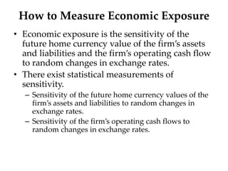
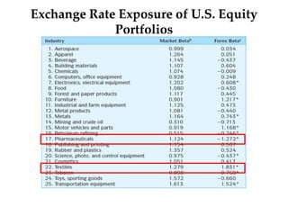
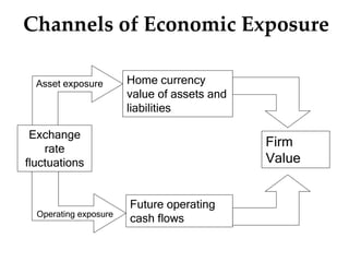
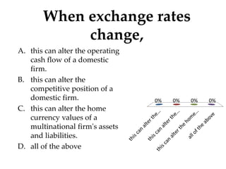
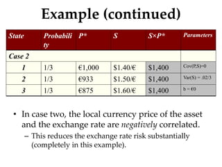
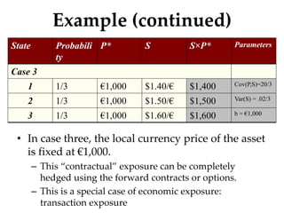
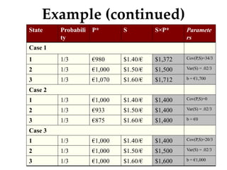
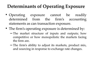
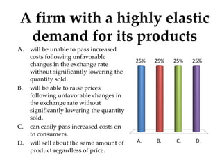
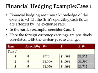
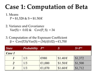
This document discusses various types of exchange rate exposure that firms face: 1. Economic exposure is how changes in exchange rates can affect the competitive position and value of domestic firms through international competition, even if they do not directly import or export. 2. Operating exposure is how exchange rate changes affect a firm's operating cash flows through factors like input costs, ability to adjust prices, and market competitiveness. It is harder to measure than transaction exposure. 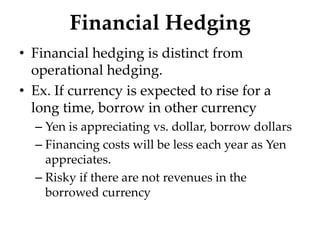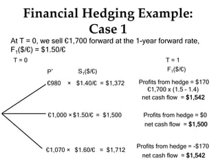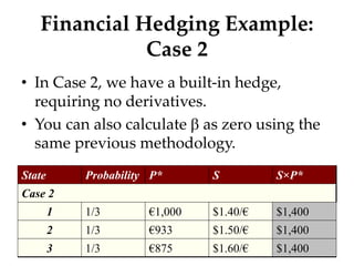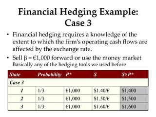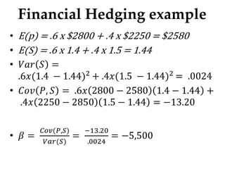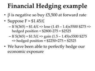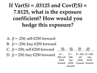3. Financial tools like hedging contracts can help manage operating and economic exposure by offsetting the effects of exchange rate movements on a firm's foreign currency cash flows and the value of its foreign assets and liabilities. The effectiveness of hedging depends on

1. Outline
• Economic Exposure
• Operating Exposure
• Determinants of Operating Exposure
• Managing Operating Exposure
• Translation Exposure
• Translation Methods
• Managing Translation Exposure

2. Economic Exposure
• Changes in exchange rates can affect not
only firms that are directly engaged in
international trade but also purely
domestic firms.
• If the domestic firm’s products compete
with imported goods, then their
competitive position is affected by the
strength or weakness of the local currency.

3. Economic Exposure
• Consider a U.S. bicycle manufacturer who
sources, produces, and sells only in the
U.S.
• Since the firm’s product competes against
imported bicycles, it is subject to foreign
exchange exposure.
– Their customers are comparing the cost and
features of the domestic bicycle against
Japanese, British, and Italian bicycles.

4. Economic Exposure
• Exchange rate risk is applied to the firm’s
competitive position.
• Any anticipated changes in the exchange rates
would already have been discounted and
reflected in the firm’s value.
• Economic exposure can be defined as the extent
to which the value of the firm would be affected
by unanticipated changes in exchange rates.

5. How to Measure Economic Exposure
• Economic exposure is the sensitivity of the
future home currency value of the firm’s assets
and liabilities and the firm’s operating cash flow
to random changes in exchange rates.
• There exist statistical measurements of
sensitivity.
– Sensitivity of the future home currency values of the
firm’s assets and liabilities to random changes in
exchange rates.
– Sensitivity of the firm’s operating cash flows to
random changes in exchange rates.

6. Exchange Rate Exposure of U.S. Equity
Portfolios

7. Asset exposure
Operating exposure
Channels of Economic Exposure
Firm
Value
Home currency
value of assets and
liabilities
Future operating
cash flows
Exchange
rate
fluctuations

8. 0% 0% 0% 0%
When exchange rates
change,
A. this can alter the operating
cash flow of a domestic
firm.
B. this can alter the
competitive position of a
domestic firm.
C. this can alter the home
currency values of a
multinational firm's assets
and liabilities.
D. all of the above

9. How to Measure Economic Exposure
• If a U.S. MNC were to run a regression on the
dollar value (P) of its British assets on the dollar-
pound exchange rate, S($/£), the regression
would be of the form:
P = a + b × S + e
Where
a is the regression constant.
e is the random error term with mean zero.
the regression coefficient b measures the sensitivity of the
dollar value of the assets (P) to the exchange rate, S.

10. How to Measure Economic Exposure
The exposure coefficient, b, is defined as
follows:
Where Cov(P,S) is the covariance between the
dollar value of the asset and the exchange rate,
and Var(S) is the variance of the exchange rate.
Cov(P,S)
Var(S)
b =

11. How to Measure Economic Exposure
• The exposure coefficient shows that there
are two sources of economic exposure:
Cov(P,S)
Var(S)
b =
1. The variance of the exchange rate.
2. The covariance between the dollar value of the
asset and exchange rate.

12. Example
• Suppose a U.S. firm has an asset in France whose
local currency price is random.
• For simplicity, suppose there are only three
states of the world and each state is equally
likely to occur.
• The future local currency price of this French
asset (P*) as well as the future exchange rate (S)
will be determined, depending on the realized
state of the world.

13. Example (continued)
• In case one, the local currency price of the asset
and the exchange rate are positively correlated.
– This gives rise to substantial exchange rate risk.
State Probabili
ty
P* S S×P* Parameters
Case 1
1 1/3 €980 $1.40/€ $1,372 Cov(P,S)=34/3
2 1/3 €1,000 $1.50/€ $1,500 Var(S) = .02/3
3 1/3 €1,070 $1.60/€ $1,712 b = €1,700

14. Example (continued)
• In case two, the local currency price of the asset
and the exchange rate are negatively correlated.
– This reduces the exchange rate risk substantially
(completely in this example).
State Probabili
ty
P* S S×P* Parameters
Case 2
1 1/3 €1,000 $1.40/€ $1,400 Cov(P,S)=0
2 1/3 €933 $1.50/€ $1,400 Var(S) = .02/3
3 1/3 €875 $1.60/€ $1,400 b = €0

15. Example (continued)
• In case three, the local currency price of the asset
is fixed at €1,000.
– This “contractual” exposure can be completely
hedged using the forward contracts or options.
– This is a special case of economic exposure:
transaction exposure
State Probabili
ty
P* S S×P* Parameters
Case 3
1 1/3 €1,000 $1.40/€ $1,400 Cov(P,S)=20/3
2 1/3 €1,000 $1.50/€ $1,500 Var(S) = .02/3
3 1/3 €1,000 $1.60/€ $1,600 b = €1,000

16. Example (continued)
State Probabili
ty
P* S S×P* Paramete
rs
Case 1
1 1/3 €980 $1.40/€ $1,372 Cov(P,S)=34/3
2 1/3 €1,000 $1.50/€ $1,500 Var(S) = .02/3
3 1/3 €1,070 $1.60/€ $1,712 b = €1,700
Case 2
1 1/3 €1,000 $1.40/€ $1,400 Cov(P,S)=0
2 1/3 €933 $1.50/€ $1,400 Var(S) = .02/3
3 1/3 €875 $1.60/€ $1,400 b = €0
Case 3
1 1/3 €1,000 $1.40/€ $1,400 Cov(P,S)=20/3
2 1/3 €1,000 $1.50/€ $1,500 Var(S) = .02/3
3 1/3 €1,000 $1.60/€ $1,600 b = €1,000

17. Operating Exposure: Definition
• The effect of random changes in exchange
rates on the firm’s competitive position,
which is not readily measurable.
– How do changing exchange rates affect the
value of the firm?
• A good definition of operating exposure is
the extent to which the firm’s operating
cash flows are affected by the exchange
rate.

18. Determinants of Operating Exposure
• Operating exposure cannot be readily
determined from the firm’s accounting
statements as can transaction exposure.
• The firm’s operating exposure is determined by:
– The market structure of inputs and outputs; how
competitive or how monopolistic the markets facing
the firm are.
– The firm’s ability to adjust its markets, product mix,
and sourcing in response to exchange rate changes.

19. Operating Exposure
• Where does the output go?
– Domestic market or export market
• In the local market, do competitors have
the same FX costs?
– Competitors who import may benefit from
their own currency depreciating
• Undifferentiated products?
– Price-sensitive or insensitive product

20. Operating Exposure
• Exporting can benefit from own currency
depreciation
– Can lower foreign prices to better compete if
price-sensitive demand
– If price-insensitive no need to lower prices,
possible windfall profits
• Where do competitors come from?
– Face same currency movements?
• Where do inputs come from?
– Imported or local? Same place as revenues?

21. Managing Operating Exposure
• Flexible Sourcing Policy
• Selecting Low Cost Production Sites
• R&D and Product Differentiation
• Financial Hedging

22. Flexible Sourcing Policy
• Currency mismatch between export
revenues and manufacturing costs can be
a large problem
– Build in one place, sell in another
– Exposed to FX movements
– Source key parts from same place/currency as
revenues are derived
– Match costs and revenues in same currency
• Not the same as outsourcing from low-
cost countries

23. Flexible Sourcing Policy
• A firm may wish to diversify the location
of its production sites to mitigate the effect
of exchange rate movements.
• More expensive than sourcing in different
countries, have to build factories
• Ex. Japanese and German car companies
in the southern U.S.
– Added benefit of costs and revenues in same
currency

24. Selecting Low Cost Production
Sites
• A lot of manufacturing has moved to
lower cost countries
– Especially true for labor-intensive production
– Move to Mexico => Taiwan/South Korea =>
China/Vietnam => Africa?
• If you don’t sell a lot in the country, you
are exposed to FX risk
– Costs in pesos, revenues in dollars/euros
– Increase peso revenues to hedge

25. Selecting Low Cost Production
Sites
• There has also been a lot of out-sourcing
• Instead of building a factory in a cheap
location, contract with someone else
– IPhones in China
• Likely not exposed to FX risk
– Pay contractor in dollars
– They are exposed to FX risk

26. R&D and Product Differentiation
• Successful research and development
(R&D) allows for:
– Cost-cutting
– Enhanced productivity
– Product differentiation
• Successful product differentiation gives
the firm less elastic demand—which may
translate into less exchange rate risk.
– Toyota and Lexus
– Honda and Acura

27. A. B. C. D.
25% 25% 25% 25%
A firm with a highly elastic
demand for its products
A. will be unable to pass increased
costs following unfavorable
changes in the exchange rate
without significantly lowering the
quantity sold.
B. will be able to raise prices
following unfavorable changes in
the exchange rate without
significantly lowering the quantity
sold.
C. can easily pass increased costs on
to consumers.
D. will sell about the same amount of
product regardless of price.

28. Financial Hedging
• Financial hedging is distinct from
operational hedging.
• Ex. If currency is expected to rise for a
long time, borrow in other currency
– Yen is appreciating vs. dollar, borrow dollars
– Financing costs will be less each year as Yen
appreciates.
– Risky if there are not revenues in the
borrowed currency

29. A positive
correlation
A negative
correlation
No
correlation
33% 33% 33%
There are two possible states of the world,
$1/€ or $1.25/€. In the first state, your asset
will be worth €1,000. In the second state,
your asset will be worth €800. There is ___
between euro asset prices and the exchange
rate.
A. A positive
correlation
B. A negative
correlation
C. No correlation

30. 0% 0% 0%
There are two possible states of the
world, $1/€ or $1.25/€. In the first state,
your asset will be worth €1,000. In the
second state, your asset will be worth
€800. There is _____ FX risk.
A. A lot of
B. No
C. An indeterminate
amount of

31. Financial Hedging Example:Case 1
• Financial hedging requires a knowledge of the
extent to which the firm’s operating cash flows
are affected by the exchange rate.
• In the earlier example, consider Case 1.
• Here the foreign currency earnings are positively
correlated with the exchange rate changes.
State Probability P* S S×P*
Case 1
1 1/3 €980 $1.40/€ $1,372
2 1/3 €1,000 $1.50/€ $1,500
3 1/3 €1,070 $1.60/€ $1,712

32. Case 1: Computation of Beta
1. Means
P = $1,528 & S = $1.50/€
2. Variance and Covariance
Var(S) = 0.02 & Cov(Pi S) = 34
3. Computation of the Exposure Coefficient
b = Cov(P,S)/Var(S) = (34)/(0.02) = €1,700
State Probability P* S S×P*
Case 1
1 1/3 €980 $1.40/€ $1,372
2 1/3 €1,000 $1.50/€ $1,500
3 1/3 €1,070 $1.60/€ $1,712

33. Financial Hedging Example:
Case 1
T = 0 T = 1
€980
€1,000
€1,070
P* S1($/€)
$1.40/€
$1.50/€
$1.60/€
×
×
×
=
=
=
$1,372
$1,500
$1,712
At T = 0, we sell €1,700 forward at the 1-year forward rate,
F1($/€) = $1.50/€
F1($/€)
Profits from hedge = $170
€1,700 x (1.5 – 1.4)
net cash flow = $1,542
Profits from hedge = $0
net cash flow = $1,500
Profits from hedge = -$170
net cash flow = $1,542

34. Financial Hedging Example:
Case 2
• In Case 2, we have a built-in hedge,
requiring no derivatives.
• You can also calculate b as zero using the
same previous methodology.
State Probability P* S S×P*
Case 2
1 1/3 €1,000 $1.40/€ $1,400
2 1/3 €933 $1.50/€ $1,400
3 1/3 €875 $1.60/€ $1,400

35. Financial Hedging Example:
Case 3
• Financial hedging requires a knowledge of the
extent to which the firm’s operating cash flows are
affected by the exchange rate.
• Sell b = €1,000 forward or use the money market
Basically any of the hedging tools we used before
State Probability P* S S×P*
Case 3
1 1/3 €1,000 $1.40/€ $1,400
2 1/3 €1,000 $1.50/€ $1,500
3 1/3 €1,000 $1.60/€ $1,600

36. Financial Hedging example
• A U.S. company owns land in London that
will likely be sold in the next year.
• Assume there are two possible states of
the world
– 60% - S(365) = $1.4/£ & land is worth £2,000
– 40% - S(365) = $1.5/£ & land is worth £1,500
• What are the potential dollar amounts?
– £2,000 x $1.4/£ = $2,800
– £1,500 x $1.5/£ = $2,250
– Clearly there is exposure to FX risk

37. Financial Hedging example
• E(p) = .6 x $2800 + .4 x $2250 = $2580
• E(S) = .6 x 1.4 + .4 x 1.5 = 1.44
• 𝑉𝑎𝑟 𝑆 =
.6𝑥(1.4 − 1.44)2
+ .4𝑥(1.5 − 1.44)2
= .0024
• 𝐶𝑜𝑣 𝑃, 𝑆 = .6𝑥 2800 − 2580 1.4 − 1.44 +
.4𝑥 2250 − 2850 1.5 − 1.44 = −13.20
• 𝛽 =
𝐶𝑜𝑣(𝑃,𝑆)
𝑉𝑎𝑟(𝑆)
=
−13.20
.0024
= −5,500

38. Financial Hedging example
• β is negative so buy £5,500 at forward rate
• Suppose F = $1.45/£
– If S(365) = $1.4/£ => lose (1.45 – 1.4)x5500 $275 =>
hedged position = $2800-275 = $2525
– If S(365) = $1.5/£ => gain (1.5 – 1.45)x5500 $275
=> hedged position = $2250+275 = $2525
• We have been able to perfectly hedge our
economic exposure

39. 0% 0% 0%
There are two possible states of the
world, $1/€ or $1.25/€. In the first state,
your asset will be worth €1,000. In the
second state, your asset will be worth
€900. There is ___ FX risk.
A. A lot of
B. No
C. An indeterminate
amount of

40. β = -
250; sell
€250
forward
β = -
250;
buy
€250
forward
β = 250;
sell
€250
forward
β = 250;
buy
€250
forward
0% 0% 0% 0%
If Var(S) = .03125 and Cov(P,S) =
7.8125, what is the exposure
coefficient? How would you
hedge this exposure?
A. β = -250; sell €250 forward
B. β = -250; buy €250 forward
C. β = 250; sell €250 forward
D. β = 250; buy €250 forward

41. $1,025;
$1,125
$1,000;
$1,125
$1,025;
$1,087
$975;
$1,163
$1,062;
$1,062
0% 0% 0% 0% 0%
For the firm above, with a 𝛽= €250. There are two
possible states of the world, $1/€ or $1.25/€. In the
first state, your asset will be worth €1,000. In the
second state, your asset will be worth €900.
Assume F = $1.10/€, what are the hedged
positions in the two possible states?
A. $1,025; $1,125
B. $1,000; $1,125
C. $1,025; $1,087
D. $975; $1,163
E. $1,062; $1,062