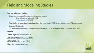
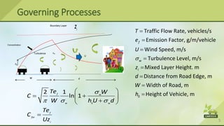
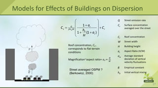
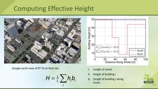
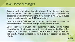
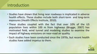
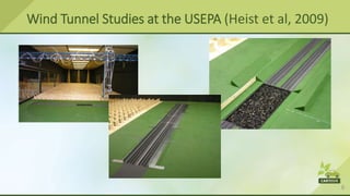
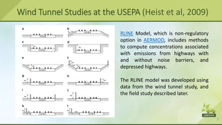
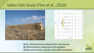
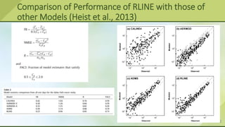
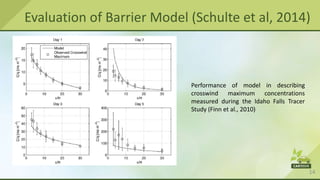
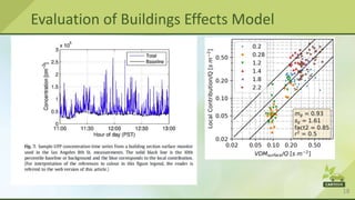
1. The document discusses methods for modeling the dispersion of air pollutants from roadways using field studies, wind tunnel experiments, and computational models. It describes several models used to simulate dispersion under various conditions like stable/unstable atmospheric conditions, presence of barriers, and effects of buildings. 2. Recent field studies and wind tunnel experiments have provided data to develop and evaluate models like RLINE that estimate near-road pollutant concentrations. These models are now incorporated into frameworks to analyze impacts on air quality and public health. 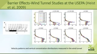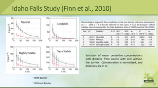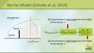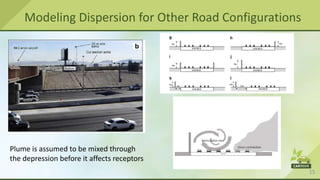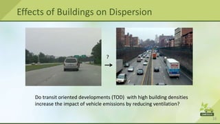3. Remaining challenges include improving models for situations like depressed roads, accounting for effects of vegetation barriers, pollutant chemistry, and micrometeorology in urban areas. Models also tend to over

1. 1
Center for Advancing Research
in Transportation Emissions,
Energy, and Health
A USDOT University Transportation Center
www.carteeh.org

2. 2
Lecture #15: Air Pollution Dispersion Modeling
Methods and Data Sources
Akula Venkatram
University of California, Riverside, CA
venky@engr.ucr.edu, 951-827-2195
The author declares that there is no conflict of interest
Lecture Tracks: HT/TT

3. 3
• Studies have shown that living near roadways is implicated in adverse
health effects. These studies include both short-term and long-term
exposures (Health Effects Institute, 2010).
• These studies coupled with the fact that over 10% of the US
population lives within 100 m from highways (Brugge, 2007) has
motivated field, wind tunnel and modeling studies to examine the
impact of highway emissions on near-road air quality.
• Such studies have been conducted since the 1970s, but recent health
studies have added impetus to them.
Introduction

4. 4
Field and Laboratory Studies
• Dispersion of releases from sources close to the ground
• Green Glow, Prairie Grass (1956)
• Project Sagebrush (2013)
• Field studies to understand road dispersion –GM tracer study (1980)- tracer released from 352 automobiles
• New road field studies
• Caltrans (Benson,1989), Raleigh study (Baldauf et al., 2008), Idaho Falls Study (2008, Finn et al. 2010)
Models
 EPA Highway Model (1970s)
 CALINE Model (Benson, 1989)
 RLINE (Snyder et al., 2013)
 C-LINE (Barzyk et al, 2013
Field and Modeling Studies

5. 5
Governing Processes
d
Boundary Layer
U
𝜎𝑤
Turbulence
h0
W
Concentration
i
z

  
 
 
 

 

0
2 1
ln 1
f w
w w
f
far
i
Te W
C
W h U d
Te
C
Uz









0
Traffic Flow Rate, vehicles/s
Emission Factor, g/m/vehicle
Wind Speed, m/s
Turbulence Level, m/s
Mixed Layer Height. m
Distance from Road Edge, m
Width of Road, m
Height of Vehicle, m
f
w
i
T
e
U
z
d
W
h

6. 6
Wind Tunnel Studies at the USEPA (Heist et al, 2009)

7. 7
Wind Tunnel Studies at the USEPA (Heist et al, 2009)
RLINE Model, which is non-regulatory
option in AERMOD, includes methods
to compute concentrations associated
with emissions from highways with
and without noise barriers, and
depressed highways.
The RLINE model was developed using
data from the wind tunnel study, and
the field study described later.

8. 8
Barrier Effects-Wind Tunnel Studies at the USEPA (Heist
et al, 2009)
Velocity patterns and vertical concentration distributions measured in the wind tunnel

9. 9
Idaho Falls Study (Finn et al., 2010)
 SF6 simultaneously released from two sources
 Concentrations measured at 56 receptors
 Spanned neutral, unstable, and stable conditions

10. 10
Idaho Falls Study (Finn et al., 2010)
- With Barrier
-Without Barrier
Neutral
Unstable
Slightly Stable
Very Stable
Variation of mean centerline concentrations
with distance from source with and without
the barrier. Concentration is normalized, and
distances are in m.

11. 11
Reformulation of Plume Spreads for Flat Terrain
(Venkatram et al., 2013)


 
 
 
 
 
 
 
 
1
2/3
* *
0.57 1 3
z
u u x
x
U U L
 
 
 
 
 
 
*
1.6 1 2.5
v z
y z
u L
Stable Conditions Unstable Conditions
 
 
 
 
 
 
 
 
 
 
*
0.57 1 1.5
z
u u x
x
U U L
 
 

 
 
 
 
1/2
*
1.6 1 0.5
| |
v z
y z
u L

12. 12
Comparison of Performance of RLINE with those of
other Models (Heist et al., 2013)

13. 13
Barrier Model (Schulte et al, 2014)
 Concentration is well mixed over the height
of the barrier, H
𝑈𝜎𝑧𝑏𝑎𝑟𝑟𝑖𝑒𝑟(𝑥) = 𝑈 𝑧𝑒𝑓𝑓 𝛼𝜎𝑧 𝑥 + 𝑈
𝐻
2
𝜋
2
𝐻
 Concentration is well mixed over the height
of the barrier, H

14. 14
Evaluation of Barrier Model (Schulte et al, 2014)
Performance of model in describing
crosswind maximum concentrations
measured during the Idaho Falls Tracer
Study (Finn et al., 2010)

15. 15
Modeling Dispersion for Other Road Configurations
Plume is assumed to be mixed through
the depression before it affects receptors

16. 16
Effects of Buildings on Dispersion
?
Do transit oriented developments (TOD) with high building densities
increase the impact of vehicle emissions by reducing ventilation?

17. 17
Models for Effects of Buildings on Dispersion
Q Street emission rate
Cs
Surface concentration
averaged over the street
Cr
Roof concentration
W Street width
H Building height
ar
Aspect Ratio (H/W)
σw
Average standard
deviation of vertical
velocity fluctuations
β Empirical constant
h0
Initial vertical mixing
Roof concentration, 𝐶𝑟,
corresponds to flat terrain
conditions
Street averaged OSPM ?
(Berkowicz, 2000)

 
 

 
 
 
 
 
0
1
1 (1 )
w
Q r
s r
W
r
a
C C
h
a
H
Magnification~aspect ratio= 𝑎𝑟=
𝐻
𝑊

18. 18
Evaluation of Buildings Effects Model

19. 19
Computing Effective Height
L Length of street
hi Height of building i
bi Length of building i along
street
 
1
i i
L
i
H hb
Google earth view of 8th St LA field site.

20. 20
Discussion
Models such as RLINE and AERMOD have now been incorporated
into comprehensive frameworks that enables policy makers to
analyze the “chain effect of transportation demand on air quality
and population health exposure” (Vallamsundar et al., 2016).
However, such frameworks are computationally demanding if the
urban area being studied involves a large number of road links.
Models such as C-LINE (Barzyk et al., 2015) are available to
overcome this problem. This model uses an analytical version of
RLINE that requires computational resources that are at least an
order of magnitude smaller than the version of RLINE that uses
numerical integration.

21. 21
• Models for dispersion from different road configurations-elevated,
depressed roads-need improvement and evaluation with observations
• Models for building effects require more evaluation before they cab be
applied in a regulatory context.
• Models overestimate concentrations under low wind speeds (Askariyeh et
al., 2017). Need methods to account for wind meandering under these
conditions.
• Need methods to account for
• Conversion of NOx to NO2
• Impact of porous vegetative barriers
• Estimating “edge” effect of roadside barriers
• Estimating micrometeorological model inputs in urban areas
Research Gaps and Future Directions

22. 22
• Current models for dispersion of emissions from highways with and
without barriers provide adequate estimates of concentrations
associated with highway emissions. New version of AERMOD includes
a non-regulatory option for RLINE application.
• Data sets from field and wind tunnel studies are available for
development and evaluation of highway dispersion models.
• Street canyons between tall buildings magnify traffic-related
concentrations that would occur in the absence of buildings. The
magnification depends on the ratio of the effective height to width of
the street. Available dispersion models do not account or building
effects.
Take-Home Messages

23. 23
AERMOD- AMS/EPA Regulatory Model
AMS- American Meteorological Society
CFD-Computational Fluid Dynamics
OSPM- Operational Street Pollution Model
RLINE- Research Line Source Dispersion Model
USEPA- United States Environmental Protection Agency
List of Abbreviations

24. 24
Ahangar, F.E., Heist, D., Perry, S. and Venkatram, A., 2017. Reduction of air pollution levels downwind of a road with an upwind noise
barrier. Atmospheric Environment, 155, pp.1-10.
Amini, S., Ahangar, F.E., Schulte, N. and Venkatram, A., 2016. Using models to interpret the impact of roadside barriers on near-road air
quality. Atmospheric Environment, 138, pp.55-64.
Amini, S., Enayati Ahangar, F., Heist, D., Perry, S., Venkatram, A., 2018. Modeling Dispersion of Emissions from Depressed Roadways. Atmos. Environ.
186, 189–197. https://doi.org/10.1016/j.atmosenv.2018.04.058
Askariyeh, M.H., Kota, S.H., Vallamsundar, S., Zietsman, J., Ying, Q., 2017. AERMOD for near-road pollutant dispersion: Evaluation of model performance with different
emission source representations and low wind options. Transp. Res. Part D Transp. Environ. 57, 392–402. https://doi.org/10.1016/j.trd.2017.10.008
Baldauf, R., Thoma, E., Khlystov, A., Isakov, V., Bowker, G., Long, T., Snow, R., 2008. Impacts of noise barriers on near-road air quality. Atmos. Environ.
42, 7502–7507. https://doi.org/10.1016/j.atmosenv.2008.05.051
Baldauf, R.W., Heist, D., Isakov, V., Perry, S., Hagler, G.S.W., Kimbrough, S., Shores, R., Black, K., Brixey, L., 2013. Air quality variability near a highway
in a complex urban environment. Atmos. Environ. 64, 169–178. doi:10.1016/j.atmosenv.2012.09.054
Barad, M., 1958. Project Prairie Grass. a Field Program in Diffusion AFCRF-tr-58-235.
Barzyk, T.M., Isakov, V., Arunachalam, S., Venkatram, A., Cook, R., Naess, B., 2015. A near-road modeling system for community-scale assessments
oftraffic-related air pollution in the United States. Environ. Model. Softw. 66, 46–56. https://doi.org/10.1016/j.envsoft.2014.12.004
Benson, P.E., 1989. CALINE3—A Versatile Dispersion Model for Predicting Air Pollutant Levels Near Highways and Arterial Streets. Interim Report,
Report. Number FHWA/CA/TL-79/23. Federal Highway Administration, Washington, DC (NTIS No. PB 80-220841).
Berkowicz, R., 2000. OSPM - A Parameterised Street Pollution Model. Environmental Monitoring and Assessment 65: 323–331, 2000
Brugge, D., Durant, J.L., Rioux, C., 2007. Near-highway pollutants in motor vehicle exhaust: a review of epidemiologic evidence of cardiac and pulmonary health risks.
Environ. Health: Glob. Access Sci. Source 6 23–23
Deshmukh, P., Isakov, V., Venkatram, A., Yang, B., Zhang, K.M., Logan, R., Baldauf, R., 2019. The effects of roadside vegetation characteristics on local,
near-road air quality. AIR Qual. Atmos. Heal. 12, 259–270. https://doi.org/10.1007/s11869-018-0651-8
Eckman, R.M., 1994. Re-examination of empirically derived formulas for horizontal diffusion from surface sources. Atmos. Environ. 28, 265–272.
https://doi.org/10.1016/1352-2310(94)90101-5
References

25. 25
Finn, D., Clawson, K.L., Carter, R.G., Rich, J.D., Eckman, R.M., Perry, S.G., Isakov, V., Heist, D.K., 2010. Tracer studies to characterize the effects of
roadside noise barriers on near-road pollutant dispersion under varying atmospheric stability conditions. Atmos. Environ. 44, 204–214.
doi:10.1016/j.atmosenv.2009.10.012
Gallagher, J., Baldauf, R., Fuller, C.H., Kumar, P., Gill, L.W., McNabola, A., 2015. Passive methods for improving air quality in the built environment: A
review of porous and solid barriers. Atmos. Environ.
Hagler, G.S.W., Tang, W., Freeman, M.J., Heist, D.K., Perry, S.G., Vette, A.F., 2011. Model evaluation of roadside barrier impact on near-road air
pollution. Atmos. Environ. 45, 2522–2530. https://doi.org/10.1016/j.atmosenv.2011.02.030
Heist, D., Isakov, V., Perry, S., Snyder, M., Venkatram, A., Hood, C., Stocker, J., Carruthers, D., Arunachalam, S., Owen, R.C., 2013. Estimating near-
road pollutant dispersion: A model inter-comparison. Transp. Res. Part D Transp. Environ. 25, 93–105. https://doi.org/10.1016/j.trd.2013.09.003
Heist, D.K., Perry, S.G., Brixey, L.A., 2009. A wind tunnel study of the effect of roadway configurations on the dispersion of traffic-related pollution. Atmos.
Environ. 43, 5101–5111. https://doi.org/10.1016/j.atmosenv.2009.06.034
Luhar, A.K., Venkatram, A., Lee, S.-M., 2006. On relationships between urban and rural near-surface meteorology for diffusion applications. Atmos.
Environ. 40. https://doi.org/10.1016/j.atmosenv.2006.05.067
Schulte, N., Snyder, M., Isakov, V., Heist, D. and Venkatram, A., 2014. Effects of solid barriers on dispersion of roadway emissions. Atmospheric
Environment, 97, pp.286-295.
Schulte, N., Tan, S., Venkatram, A., 2015. The ratio of effective building height to street width governs dispersion of local vehicle emissions. Atmos.
Environ. 112. doi:10.1016/j.atmosenv.2015.03.061
Snyder, M.G., Venkatram, A., Heist, D.K., Perry, S.G., Petersen, W.B. and Isakov, V., 2013. RLINE: A line source dispersion model for near-surface
releases. Atmospheric environment, 77, pp.748-756.
Valencia, A., Venkatram, A., Heist, D., Carruthers, D., Arunachalam, S., 2018. Development and evaluation of the R-LINE model algorithms to account for
chemical transformation in the near-road environment. Transp. Res. Part D Transp. Environ. 59, 464–477. https://doi.org/10.1016/j.trd.2018.01.028
Vallamsundar, S., Lin, J., Konduri, K., Zhou, X., Pendyala, R.M., 2016. A comprehensive modeling framework for transportation-induced population exposure
assessment. Transp. Res. Part D Transp. Environ. 46, 94–113. https://doi.org/10.1016/j.trd.2016.03.009
Venkatram, A., Horst, T.W., 2006. Approximating dispersion from a finite line source. Atmos. Environ. 40. https://doi.org/10.1016/j.atmosenv.2005.12.014
References

26. 26
Venkatram, A., Snyder, M., Isakov, V., Kimbrough, S., 2013. Impact of wind direction on near-road pollutant concentrations. Atmos. Environ. 80, 248–258.
https://doi.org/10.1016/j.atmosenv.2013.07.073
Venkatram, A., Snyder, M., Isakov, V., Kimbrough, S., 2013. Impact of wind direction on near-road pollutant concentrations. Atmos. Environ. 80, 248–258.
https://doi.org/10.1016/j.atmosenv.2013.07.073
Venkatram, A., Snyder, M.G., Heist, D.K., Perry, S.G., Petersen, W.B., Isakov, V., 2013. Re-formulation of plume spread for near-surface dispersion.
Atmos. Environ. 77, 846–855. doi:10.1016/j.atmosenv.2013.05.073
Wang, Y.J., Zhang, K.M.A.X., 2009. Modeling Near-Road Air Quality Using a Computational Fluid Dynamics Model , CFD-VIT-RIT 43, ES&T, 43, 7778–
7783.
References

27. 27
• Cimorelli, A.J., Perry, S.G., Venkatram, A., Weil, J.C., Paine, R.J.,
Wilson, R.B., Lee, R.F., Peters, W.D., Brode, R.W., 2005. AERMOD: A
dispersion model for industrial source applications. Part I: General
model formulation and boundary layer characterization. J. Appl.
Meteorol. 44. https://doi.org/10.1175/JAM2227.1
• Venkatram, A., and Schulte, N., 2018. Urban Transportation and Air
Pollution. Elsevier, ISBN-13: 978-0128115060
Reading List

28. 28
Research funded by South Coast Air Quality Management District,
California Air Resources Board, California Energy Commission, National
Science Foundation, and US Environmental Protection Agency
Collaborators: Marko Princevac, David Pankratz, Dennis Fitz, Jeffrey
Weil, Steven Perry, David Heist, Alan Cimorelli, Roger Brode, Richard
Baldauf, Vlad Isakov, Parikh Deshmukh, Steven Hanna, Sarav
Arunachalam, Sang-Mi Lee, Shuming Du
Students: Nico Schulte, Seyedmorteza Amini, Faraz Ahangar, Wenjun
Qian, Jing Yuan
Acknowledgements