14463

Learning strategies in amnesia

Maarten Speekenbrink, Shelley Channon and David R. Shanks
Department of Psychology
University College London

Abstract
Previous research suggests that early performance of amnesic individuals in
a probabilistic category learning task is relatively unimpaired. When com-
bined with impaired declarative knowledge, this is taken as evidence for the
existence of separate implicit and explicit memory systems. The present
study contains a more fine-grained analysis of learning than earlier studies.
Using a dynamic lens model approach with plausible learning models, we
found that the learning process is indeed indistinguishable between an am-
nesic and control group. However, in contrast to earlier findings, we found
that explicit knowledge of the task structure is also good in both the amnesic
and the control group. This is inconsistent with a crucial prediction from the
multiple-systems account. The results can be explained from a single system
account and previously found differences in later categorization performance
can be accounted for by a difference in learning rate.

Over the past decades, neuropsychology has shown increasing interest in probabilistic cat-
egory learning. In a widely-used categorization task, known as the “weather prediction”
task (Knowlton, Squire, & Gluck, 1994), the objective is to predict the weather (sunny or
rainy) on the basis of four cues (tarot cards with different geometric patterns). Introducing
the task as a variant of the medical diagnosis task (Gluck & Bower, 1988), Knowlton et al.
(1994) found that, relative to controls, early categorization performance was not impaired
in amnesia. Amnesic patients with medial temporal lobe or diencephalic lesions showed ap-
parent normal learning, despite their severe declarative memory problems. One explanation
for this finding, favoured by many authors (e.g. Ashby, Alfonso-Reese, Turken, & Waldron,
1998; Ashby & Maddox, 2005; Gabrieli, 1998; Knowlton et al., 1994; Knowlton, Mangels,
& Squire, 1996; Poldrack & Rodriguez, 2004), is in terms of multiple memory systems.
Knowlton et al. (1994) argued that early learning in multiple cue tasks is mainly depen-
dent on procedural (implicit) memory, which is not impaired in amnesia. This hypothesis
gained further support from the “double dissociation” between categorization performance
and declarative memory. Knowlton et al. (1996) found that, while amnesic patients showed
relatively unimpaired early categorization performance, they had impaired declarative (ex-
plicit) memory for the task episode. Parkinson’s patients, who are assumed to have impaired
procedural but unimpaired declarative memory, showed relatively impaired categorization
performance from the outset, but did show accurate memory of the testing episode (Knowl-

LEARNING STRATEGIES IN AMNESIA 2

ton et al., 1996).
While this evidence is appealing, it shows weaknesses upon closer examination. The
analyses only focus on the effect of learning (categorization performance), but neglect the
underlying learning process. At present, it is unclear how individuals learn in the weather
prediction task. Moreover, the declarative knowledge tapped in the experiments referred to
irrelevant task features, rather than to the object of learning. The purpose of the present
paper is to submit the learning behaviour and declarative knowledge to a more sensitive
analysis. We analysed participants’ (amnesic and control) learning on a trial-by-trial basis
and investigated how they integrated information to arrive at their predictions. We com-
pared their performance to normative learning models, in order to gain further insight into
possible differences between amnesic and normal participants. By applying a dynamic lens
model approach, we captured the progression of participants’ implicit response strategies.
Finally, by tapping participants’ explicit knowledge regarding the task structure and their
categorization strategies, we investigated whether there is a dissociation between procedural
and declarative memory in probabilistic category learning.

Evidence for a double dissociation in probabilistic category
learning.
The empirical evidence for a double dissociation between procedural and declarative
memory concerns two groups of individuals; one group shows normal categorization perfor-
mance but impaired declarative memory of the task, while the second group shows impaired
categorization performance but unimpaired declarative knowledge of the task. In our short
review of the evidence for this dissociation, we limit discussion to research conducted with
the weather prediction task (for a more complete overview, the reader is referred to Gabrieli,
1998; Ashby & Maddox, 2005).
It is an established finding that, compared to controls, amnesic individuals show unim-
paired early learning (Knowlton et al., 1994, 1996; Eldridge, Masterman, & Knowlton, 2002;
Reber, Knowlton, & Squire, 1996; but see Hopkins, Myers, Shohamy, Grossman, & Gluck,
2004, for a different result). More specifically, what has been found is that categorization
performance of amnesic groups does not significantly differ from performance of matched
controls in the first 50 trials of the weather prediction task. Since the performance of both
groups does differ significantly from chance performance, both groups show learning, in an
apparently similar manner. However, when asked about certain features of the task, such
as where the cards were placed on a computer screen, or the number of elements of the
geometric patterns on the cards, amnesic patients show very poor memory of these task
features (Knowlton et al., 1996; Eldridge et al., 2002). Hence, there appears to be unim-
paired learning, but impaired declarative memory in amnesia. Learning, so the argument
goes, must thus be based on a procedural memory system which is independent of the me-
dial temporal lobes. Parkinson’s patients, on the other hand, show impaired categorization
performance from the outset (Knowlton et al., 1996; Shohamy, Myers, Onlaor, & Gluck,
2004), while their knowledge of task features is normal (Knowlton et al., 1996; Sage et al.,
2003). This complements the evidence, in that participants can show accurate declarative
memory of task features, while having an impaired ability to learn to categorize the stimuli.
But declarative knowledge of these task features is irrelevant (Lovibond & Shanks,
2002). To show that learning is based on a procedural memory system inaccessible to


conscious recollection, we should consider knowledge of the object of learning (i.e., the
contingencies between cards and weather). This task knowledge is to be distinguished
from another relevant type of declarative knowledge: self-insight. Self-insight refers to an
individual’s knowledge of how (s)he uses the cues in order to predict the outcome (Lagnado,
Newell, Kahan, & Shanks, 2006). In previous research, these two types of declarative
knowledge have often been conflated, and it is not clear whether the claimed dissociation
between procedural and declarative memory refers to a dissociation between classification
performance and task knowledge, classification performance and self-insight, or classification
performance, task knowledge and self-insight. To our knowledge, the effect of amnesia on
self-insight has not been investigated previously, while there has been only one study (Reber
et al., 1996) addressing amnesia and task knowledge. Reber et al. (1996) found that amnesic
patients lacked explicit knowledge of the probabilities in the task, while controls’ judged
probabilities were quite close to the objective values. However, in this study, participants
were only shown 50 trials. Although this may be enough to ensure better-than-chance
performance, it is hardly enough to gain adequate knowledge of the contingencies between
cards and weather. Some of the cue patterns for which participants were asked to rate the
probability of the outcome were shown only once; at least in a statistical sense, estimating a
probability from a single observation is highly problematic. In this light, it is not remarkable
that the amnesic participants lacked knowledge. What is more surprising is that the control
subjects knew as much as they did.
This brings us to a related problem: the results mainly concern early performance.
After more trials, categorization performance has been found to differ between amnesic and
control participants (Knowlton et al., 1994). Knowlton et al. explain this later divergence
by assuming that, as the task progressed, control participants may have formed strategies
which depend on declarative memory. Amnesic patients would not have been able to develop
such strategies. Shohamy et al. (2004) found that performance of Parkinson’s patients did
increase steadily with training, although not to the level of control subjects. They offer
a similar explanation for this finding, namely that Parkinson’s patients were apparently
able to develop declarative learning strategies. However, alternative explanations are also
consistent with this pattern. For instance, different patient groups could simply learn at
lower rates than controls (e.g., Kinder & Shanks, 2001; McClelland & Rumelhart, 1986),
which would result in more marked differences in performance as the task progresses.
Neuroimaging studies have sought more direct evidence for the involvement of dif-
ferent memory systems in the weather prediction task. Poldrack et al. (2001) compared
performance of healthy participants in two versions of the task: the standard feedback-based
version, and a paired-associate learning version, in which participants were asked to mem-
orize cue-outcome pairings. The latter version was designed to engage declarative memory.
In a subsequent test phase, participants in both conditions showed equal categorization
performance, but differences in neuronal activity: relative to a baseline task, participants
who learned the feedback-based version showed more activity in the caudate nucleus, and
less activity in the medial temporal lobe (MTL), while participants who learned the paired
associate version showed the opposite pattern. Furthermore, a second experiment with just
the feedback-based version showed that the MTL was initially active, and the caudate nu-
cleus inactive, but this pattern was quickly reversed, with the MTL becoming inactive, and
the caudate nucleus active. On the basis of these findings, Poldrack et al. (2001) propose


a competition between MTL- and striatum-based memory systems in probabilistic cate-
gory learning. According to this account, the MTL acquires flexible, relational knowledge,
while the striatum acquires inflexible stimulus-response associations. Competition is neces-
sitated by the assumed fundamental incompatibility of these types of information. Foerde,
Knowlton, and Poldrack (2006) tried to increase reliance on implicit memory by assigning
participants a secondary task. They showed that performance was not different under single
or dual task conditions, but that the secondary task impaired declarative knowledge of the
cue-outcome contingencies. Moreover, single and dual task learning resulted in different
neuronal activity; performance on items learned under single task conditions was correlated
with activity in the right hippocampus, while performance on items learned under dual task
conditions was correlated with activity in the putamen.
While these neuroimaging studies have shown the involvement of both the MTL and
striatum in the weather prediction task, and that their relative involvement can be mod-
ulated by task demands, whether they provide evidence for separate implicit and explicit
memory/learning systems is debatable. Implicit memory entails a lack of explicit knowl-
edge, and while Foerde et al. (2006) found impaired declarative knowledge under dual task
conditions, Newell, Lagnado, and Shanks (in press) failed to replicate this finding in a sim-
ilar experiment. Moreover, contrary to Foerde et al., the dual task condition performed
significantly below the single task condition. In a second experiment, Newell et al. (in
press) found that participants in a feedback- and observation-based version of the weather
prediction task did not differ in declarative knowledge, which is unexpected if participants
relied on different memory systems. As such, it is questionable whether the manipulations
were successful in engaging implicit learning, and thus, whether the differences in neuronal
activity reflect different memory systems. By itself, that task demands engage distinct re-
gions of the brain does not imply the involvement of different memory systems (Sherry &
Schacter, 1987).
To summarize, the evidence for multiple memory systems is weak. Claims of dis-
sociable implicit and explicit memory systems rely on strong assumptions, such as the
inaccessibility to conscious recollection. Valid tests of these assumptions have been rare
and inconclusive. The empirical data do not rule out the possibility that individuals learn
in qualitatively similar ways, but that a neurological disorder (amnesia, or Parkinson’s dis-
ease) affects the rate of learning. This quantitative difference should affect procedural and
declarative memory alike (given that both pertain to the same object, i.e., the contingencies
in the environment). In contrast to this single system explanation, a multiple memory sys-
tems account would predict that individuals learn in qualitatively different ways (depending
on the memory system involved), or that performance on implicit and explicit tests relies
on different memory systems. To test these different hypotheses, we need to investigate the
learning process directly, and employ valid tests of procedural and declarative memory.

Learning strategies
The strategies employed in solving probabilistic category learning tasks were inves-
tigated by Gluck, Shohamy, and Myers (2002). Based on participants’ self-reports, they
formulated three broad learning strategies and compared how well these described partici-
pants’ categorization behaviour. Overall, participants seemed to adopt a singleton strategy,
in which they predicted the optimal outcome for singleton patterns (patterns in which only


a single cue is present), and guessed for other patterns. It was also apparent that strategy
use changed during the task. Towards the end of the task, a large proportion of partici-
pants seemed to adopt a multi-cue strategy, in which predictions were based on all available
cues. The paradigm has later been used to distinguish learning strategies of different pa-
tient groups (e.g. Hopkins et al., 2004; Shohamy et al., 2004). In particular, Hopkins et al.
(2004) found that amnesic patients overwhelmingly used a singleton strategy, while controls
showed more variety in their strategies.
There is reason to question the validity of the strategies defined by Gluck et al.
(2002). A main problem of the multi-cue strategy as formulated by Gluck et al. is that it is
a deterministic strategy (i.e., for each cue pattern for which the probability of an outcome
is greater than .5, a participant is taken to predict that outcome with probability 1). This
is also known as a maximising strategy. It has been shown often that participants fail
to follow this (optimal) maximising strategy, even when they know the structure of the
task. Participants often show a probability matching strategy, in which the probability of a
particular response is close to the probability that this response is correct (Shanks, Tunney,
& McCarthy, 2002). Hence, the poor fit of the multi-cue strategy could be the result of
probability matching, rather than a failure to integrate the information of all cues. Indeed,
as Lagnado et al. (2006) showed, by including a multi-cue/probability matching strategy,
the evidence for the singleton strategy vanishes, as most participants are characterised by
this multi-match strategy. Meeter, Myers, Shohamy, Hopkins, and Gluck (2006) also found
that the preponderance of the singleton strategy could be attributed to it accounting for
random and below chance responses better than the other strategies.
For our purposes, a more important problem with the strategies is that they pertain
more to response than learning processes. This distinction may seem subtle, but its im-
portance has been stressed before (e.g. Massaro & Friedman, 1990; Friedman & Massaro,
1998; Kitzis, Kelley, Berg, Massaro, & Friedman, 1998). While the learning process involves
acquiring knowledge regarding the contingencies in the environment, the response process
involves the use of this knowledge to form predictions. Strategies such as the singleton or
multi-cue strategy require knowledge of the contingencies between cues and outcome, which
can only be acquired by learning through repeated observation of cues and outcome. In
other words, the learning process is not captured by the models, which only predict the
response given that the knowledge has been acquired. The learning process may or may not
be dependent on the response process (for instance, in multiple cue learning, the feedback
governing learning is independent of the response given, while in reinforcement learning, the
response determines the subsequent reinforcement which in turn drives learning), but the
response process is usually considered to be dependent on the knowledge acquired through
learning. For probabilistic category learning, we take the view that the learning process is
primary, with the response process being dependent on it (but not vice versa). Although
the effects of the learning and response process are confounded in participants’ responses,
advances have been made to distinguish the two (e.g., Friedman, Massaro, Kitzis, & Cohen,
1995; Friedman & Massaro, 1998; Kitzis et al., 1998).
To conclude, the validity of the strategy-based account is unclear. The strategies are
partly based on self-report, but this is inconsistent with the hypothesis that probabilistic
category learning is a form of implicit learning. Explicit learning on the other hand should
result in a good correspondence between reported and employed strategy. However, Gluck


et al. (2002) found a general mismatch between reported strategy and best-fitting strategy
on the basis of formal modelling. Also, the models proposed are all of the form ‘given
pattern X the participant always responds A’, while research has consistently shown that
participants are much more variable in their responses. Finally, the strategy-based account
does not inform us how participants learn, although an improved model which allows strat-
egy switches (Meeter et al., 2006), is a step in the right direction. Hence, to study learning
strategies in amnesia, or anywhere else, we should look for a different approach. Here, we
develop formal models of learning in probabilistic categorization tasks, and then apply them
to learning data from an amnesic and control group.

Learning process
In multiple cue probability learning (MCPL) the objective is to predict the outcome
of a criterion variable y on the basis of J cues x = (x1 , . . . , xJ )T , where T denotes the
transpose. For example, in the Weather Prediction Task, the objective is to predict the
state of the weather y, which can be sunny (y = 0) or rainy (y = 1), on the basis of four
tarot cards (xj ), each of which can be presented (xj = 1) or not (xj = 0). The cues and
outcome are probabilistically related, and predictions should be based on the conditional
distribution P (y|x). By repeated observation of paired observations (y, x), it is possible
to learn the particulars of this conditional distribution, and hence to arrive at optimal
predictions. The optimal prediction for a given cue pattern x is simply to predict r = 1 if
P (y = 1|x) is larger than P (y = 0|x), and r = 0 otherwise.
We will focus on models in which the conditional probability is approximated by a
function of the cue values. When y is a binary variable, as it is here, a useful choice is the
logistic regression function

P (y = 1|x) [1 + exp(−wT x)]−1 , (1)

in which the regression weights w = (w1 , . . . , wJ )T can be estimated from repeated observa-
tions of cues and outcome. The true values of these regression weights1 reflect how well the
outcome can be predicted from the cues, and we will refer to them as cue validity weights
v. We define learning as the change in w (the current inference of v) over trials t, where
the change is in the direction of v.
We now present two models which function in this way. Both models are models
for on-line learning, by which we mean that the change in w from one trial to the next
is determined solely by the information (xt and yt ) presented at that trial. This is to be
contrasted with models for batch learning, in which the change in weights is determined by
the information from previous trials as well (usually all previous observations). The two
models presented next are normative models in the sense that they can be guaranteed to
arrive at v in the limit as t → ∞.

Associative learning
The first model is an associative model, in which the weights can be interpreted as
associations between cues xj and outcome y, which increase or decrease in strength based
1
By true values we mean the population values of the regression weights, i.e. the values of w for which
the approximation in Equation 1 is closest to the real value of P (y|x).


on the given information. At each trial t, weights are determined by changing them in the
direction which minimizes the ‘cross-entropy’ error (C. M. Bishop, 1995)

et = − yt ln f (wT xt ) + (1 − yt ) ln[1 − f (wT xt )] , (2)

in which f (·) is the logistic function of Equation 1. This leads to the following recursive
relation
wt+1 = wt + ηt [yt − f (wT xt )]xt ,
t (3)
in which ηt is the learning rate parameter which determines the size of the change in the
direction that minimises the error. When the learning rate meets certain conditions2 , it
can be shown that wt converges to v as t → ∞ (Robbins & Monro, 1951). A simple
scheme obeying these conditions is ηt = η/t. Another option, which does not guarantee
convergence, is a constant learning rate ηt = η, for which Equation 3 becomes the LMS rule
(Gluck & Bower, 1988).
It should be noted that this associative learning model is identical to a single layer
feedforward neural network with a logistic activation function. As such, it appears identical
to the model used by Gluck and Bower (1988). However, while the models are indeed very
similar, there is a crucial distinction in that, due to the logistic activation and error function
employed, this model learns the probabilities in the environment directly. Gluck and Bower’s
model used a linear activation function, incorporating a logistic transformation only ‘after
the fact’ to model probabilities of response. Moreover, we will allow for decreasing learning
rate, while the LMS learning rule used by Gluck and Bower only uses a constant learning
rate.

Bayesian learning
The second model we consider instantiates Bayesian learning. Bayesian models have
become increasingly popular, both in statistics and psychology (e.g. Anderson, 1991;
Chater, Tenenbaum, & Yuille, 2006). In the Bayesian framework, learning concerns the
distribution of parameters, rather than point estimates of the parameter values. This is
done through the recursive relation

gt (w|x1:t , y1:t ) = f (yt |xt , w)gt−1 (w|x1:t−1 , y1:t−1 )/K, (4)

in which the likelihood function f (·) is the logistic function in Equation 1, gt the posterior
density of w, gt−1 the prior density of w, and the constant K (which is computed by
integrating the right hand side of Equation 4 with respect to w) ensures that gt is a proper
probability density (i.e., it integrates to 1). Starting from a prior density g0 (w), learning
consists of determining gt at each trial t from xt , yt and gt−1 .
While the associative model accounts for decreasing weight of new observations by
a decreasing learning rate, the Bayesian model does so implicitly. Due to the nature of
Bayesian learning, the posterior becomes more and more peaked around a value of w when
more observations come in. Because of this, the relative eﬀect of a new observation on the
posterior distribution decreases. This implication is somewhat analogous to the computa-
tion of a mean: the relative weight of each observation when computing the mean from 10
2 ∞ ∞ 2
These conditions are (1) limt→∞ ηt = 0, (2) t=1 ηt = ∞, and (3) t=1 ηt < ∞.


observations is 1/10, while the relative weight is 1/100 when computing the mean from 100
observations.

Response process
When the outcome (and hence the response) is categorical, it is an established ob-
servation that P (r|xt ) is usually not identical to P (y|xt ), even though the participants
may have learned the latter probability correctly (Shanks et al., 2002). In fact, probabil-
ity matching, where the probabilities are approximately equal, is not the optimal strategy
for predicting the outcome. Maximising the probability of a correct prediction requires
P (r = j|xt ) = 1 when P (y = j|xt ) > .5. P (r|xt ) usually lies between probability matching
and this maximising strategy. In any case, it is clear that individuals differ in the way
in which they act upon learned contingencies. A particularly useful way to capture such
individual differences is to assume
P (y = 1|xt )λ
P (r = 1|xt ) = , (5)
P (y = 1|xt )λ + P (y = 0|xt )λ

in which P (y = 1|xt ) represents the model predicted probability of Equation 1 and λ > 0
is a response scaling parameter (e.g. Friedman & Massaro, 1998; Nosofsky & Zaki, 1998;
Zaki, Nosofsky, Stanton, & Cohen, 2003). When λ = 1, the response process is probability
matching, while values of λ > 1 indicate deviations towards maximising. If λ lies between
0 and 1, this indicates ‘undershooting’ so that the individual under-utilizes the learned
contingencies. When the relation in Equation 5 holds, it can be shown that u = λw (see
the Appendix), where u contains the cue utilization weights, the regression weights for the
logistic regression model for the responses (Equation 1 when the left hand side is replaced
with P (r = 1|x)). In other words, if a participant learns as the model prescribes, then the
utilization weights are a linear function of the inferred cue validity weights (the weights of
the model fitted to the outcome). The slope of this linear function is equal to λ.

Lens Model approach
The learning models and response process describe how participants respond if they
exactly follow the learning process. However, participants’ actual behaviour may deviate
from these normative models. For instance, participants may not focus on all the cues
to the same extent. As such, the utilization weights will deviate from the inferred cue
validity weights of an ideal observer. In order to investigate such discrepancies, we relied
on a lens model analysis. The lens model approach has proven a valuable tool to capture
participants’ implicit judgement policies in multiple cue tasks (for a review, see Cooksey,
1996; Goldstein, 2004). The general idea is to fit two two regression models, one regressing
the outcome y on the cues x, and the other regressing the response r on the cues. With this
approach, one can analyse performance (usually defined as the correlation between y and
r) as a function of the particulars of the environment (cues and outcome) and judgement
system (cues and response). In particular, the regression weights of the environment (v,
the true, and w, the inferred cue validity weights) are compared to those from the model
of the judgement system (u, the cue utilization weights). Recently, the approach has been
applied to study dynamical learning processes by applying the lens model to a moving


window of trials (Kelley & Friedman, 2002; Lagnado et al., 2006). This “rolling regression”
technique provides a sequence of estimates of the utilization weights and cue validities. By
comparing ut , the cue utilization weights, to wt , the inferred cue validity weights of an ideal
observer, one can investigate how the participants learned relative to how well they could
have learned.
The approach adopted here is similar in the sense that the same model is fitted to both
outcome and response. However, rather than using a rolling regression analysis, we use the
on-line learning models described previously. In this way, we try to capture more realistic
learning processes, while maintaining the ability to compare participants’ performance to
that of an ideal learning mechanism, provided with the same information.

Method
Participants
Nine participants (6m, 3f) with memory disorders took part in the study (see Table 1).
Four of these were diagnosed with alcoholic Korsakoff’s syndrome. Four had developed
memory problems from suspected temporal lobe damage following encephalitis, and MRI
radiological investigation in two of these cases confirmed medial temporal lobe involvement.
One had a right-sided medial temporal lobe tumour, confirmed by radiological investigation.
Sixteen control participants also took part in the study (7m, 9f). To be included in the
study, participants had to be between 18 and 75 years of age, fluent in English, within the
normal range on the Test of Reception of Grammar (D. V. M. Bishop, 1989), and have an IQ
score of 85 or above. Exclusion criteria included significant physical or psychiatric illness
(with the exception of the primary diagnosis for the amnesic group), hydrocephalus and
dementing conditions, and expressive or receptive aphasia. The two groups of participants
did not differ significantly (p > 0.1) in age, years of education, or Wechsler Abbreviated
Scale of Intelligence (WASI) IQ (Wechsler, 1999).
All participants were assessed on the Wechsler Memory Scale III (Wechsler, 1997),
in addition to the experimental task (Table 1). The amnesic group performed significantly
more poorly than the control group on each of these measures (p < .0001 except for the
Auditory Recognition Delayed Index and Working Memory Index, where p < .01), and de-
gree of memory impairment in individual amnesic participants ranged from mild to marked.
Participants were also tested on the Tower, Trail-Making, and Colour Word Interference
subtests of the Delis-Kaplan Executive Function System (DKEFS) test (Delis, Kaplan, &
Kramer, 2001). Results are given in Table 2. The amnesic group did not differ significantly
from the control group (p > .05) on the Tower and Trail-Making subtests, or on three of
the four components of the Colour-Word Interference subtest; they did differ significantly
on the Inhibition/switching component of the latter subtest.

Materials
The Weather Prediction task was identical to that used by Lagnado et al. (2006). The
stimuli presented to participants were taken from a set of four cards, each with a different
geometric pattern (squares, diamonds, circles, triangles). The task consisted of a total of
200 trials, on each of which participants were presented with a pattern of one, two or three
cards. Each trial was associated with one of two outcomes (Rain or Fine), and overall

Table 1: Etiology, sex, age, years of education, IQ, and Wechsler Memory Scale III scores for the amnesic and control group. WMS scales:
Auditory Immediate (AI), Auditory Delayed (AD), Auditory Recognition Delayed (ARD), Visual Immediate (VI), Visual Delayed (VD),
Immediate Memory (IM), General Memory (GM), and Working Memory (WM).
Wechsler Memory
auditory visual
etiology* sex age education IQ AI AD ARD VI VD IM GM WM
Amnesic
A1 Enceph. F 51 16 102 62 61 70 91 78 71 64 88
A2 Enceph. F 50 13 100 105 102 90 81 81 93 89 79
A3 Kors. M 51 11 87 89 83 75 88 88 86 79 83
A4 Kors. M 49 16 125 105 105 115 81 91 93 103 131
A5 Enceph. M 57 13 118 111 86 110 68 75 89 84 99
A6 MTL t. M 75 16 106 83 74 75 61 68 67 67 91
A7 Enceph. M 50 16 113 77 83 90 81 84 74 82 88
A8 Kors. F 56 16 99 62 58 80 57 65 51 60 81
A9 Kors. M 52 11 103 59 55 65 61 53 51 47 83
Mean 54.56 14.22 105.88 83.67 78.56 85.56 74.33 85.56 75.00 75.00 91.44
SD 8.14 2.22 11.32 20.24 18.20 17.40 12.72 17.40 17.03 17.03 16.02
LEARNING STRATEGIES IN AMNESIA

Control
Mean 56.75 13.94 104.50 110.38 113.44 109.06 99.88 109.06 106.69 108.00 109.31
SD 10.95 2.14 14.43 11.60 9.57 15.94 13.73 14.83 11.25 9.87 14.83

* Enceph. = Encephalitis, Kors. = alcoholic Korsakoﬀ’s syndrome, MTL t. = MTL tumour.
10


Table 2: Means and standard deviations of the Delis-Kaplan Executive Function System scales.
Amnesic Control
M SD M SD
Tower 10.89 2.47 11.27 2.15
Trail making
motor speed 9.33 3.16 10.13 1.73
visual scanning 9.00 1.50 10.31 2.60
number sequencing 10.11 1.97 10.50 2.45
letter sequencing 10.00 1.87 11.00 2.36
number-letter switching 10.22 2.77 11.25 1.92
Colour Word Interference
colour naming 8.44 3.32 10.07 3.08
colour word reading 10.67 2.12 11.20 2.83
colour inhibition 8.44 4.50 11.07 2.05
inhibition/switching 7.56 4.16 11.13 2.56

these two outcomes occurred equally often. The pattern frequencies and probabilities of
the outcome were identical to those in Gluck et al. (2002, Experiment 2) and subsequent
other studies (e.g., Hopkins et al., 2004; Lagnado et al., 2006), and are shown in Table
1, along with the probability of the outcome for each of these 14 patterns. The learning
set was constructed so that each card was associated with the outcome with a different
probability. For example, the probability of rain was .2 over all the trials on which the
squares card (card 1) was present, .4 for trials on which the diamonds card (card 2) was
present, .6 for trials on which the circles card (card 3) was present, and .8 for trials on which
the triangles card (card 4) was present. Thus, two cards were predictive of rainy weather,
one strongly (card 4), one weakly (card 3), and two cards were predictive of fine weather,
one strongly (card 1), one weakly (card 2). Overall, participants experienced identical
pattern frequencies (order randomized for each participant), but the actual outcome for
each pattern was determined probabilistically (so experienced outcomes could differ slightly
across participants). The position of the cards on the screen were held constant within
participants, but counterbalanced across participants.

Procedure

The procedure of the experiment was identical to that in Lagnado et al. (2006), and
a detailed description can be found there. Participants were given on-screen instructions,
after which they moved onto the first block of 50 trials. On each trial a specific pattern
of cards (selected from Table 3) was displayed on the screen. Participants were then asked
to predict the weather on that trial, by clicking on the corresponding button (RAINY or
FINE). Once they had made their prediction, participants received immediate feedback as
to the actual weather on that trial, and whether they were correct or incorrect.
At the end of each block of fifty trials participants answered two different sets of test
questions. In the probability test participants were asked to give probability ratings for


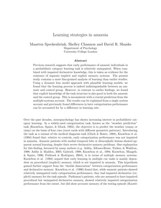
Table 3: Learning environment.
Pattern Cards present Total P(pattern) P(fine|pattern)
A 0001 19 0.095 0.895
B 0010 9 0.045 0.778
C 0011 26 0.13 0.923
D 0100 9 0.045 0.222
E 0101 12 0.06 0.833
F 0110 6 0.03 0.500
G 0111 19 0.095 0.895
H 1000 19 0.095 0.105
I 1001 6 0.03 0.500
J 1010 12 0.06 0.167
K 1011 9 0.045 0.556
L 1100 26 0.13 0.077
M 1101 9 0.045 0.444
N 1110 19 0.095 0.105
Total 200 1.00

each of the four cards. For each card they were asked for the probability of rainy vs. fine
weather: ‘On the basis of this card what do you think the weather is going to be like?’
They registered their rating using a continuous slider scale ranging from ‘Definitely fine’
to ‘Definitely rainy’, with ‘As likely fine as rainy’ as the midpoint. In the importance test
participants were asked how much they had relied on each card in making their predictions:
‘Please indicate how important this card was for making your predictions’. They registered
their rating using a continuous slider scale ranging from ‘Not important at all’ to ‘Very
important’, with ‘Moderately important’ as the midpoint.

Results
Learning Performance
It has been customary to analyse participants’ performance in terms of the proportion
of optimal responses (e.g. Hopkins et al., 2004; Knowlton et al., 1994, 1996; Shohamy et
al., 2004). However, such a measure of performance does not distinguish between optimal
responses to highly predictive versus weakly predictive patterns3 . Instead, we assessed
participant’s performance through the score statistic
T
1
S= rt P (y = 1|xt ) + (1 − rt )[1 − P (y = 1|xt )], (6)
T
t=1
3
Consider two patterns x1 and x2 . The probability of Rain given pattern 1 is .92, and given pattern 2 it
is .56. We would consider a non-optimal response (Sun) for pattern 1 as worse than a non-optimal response
(Sun) for pattern 2. This difference is not taken into account in the proportion of optimal responses. In
other words, only considering optimal responses might not distinguish between someone who always predicts
Rain to pattern 1 and Sun to pattern 2, and someone who always predicts Sun to pattern 1 and Rain to
pattern 2. However, the expected number of correct predictions is much higher for the first than for the
second person.


in which rt = {0, 1} is a participant’s response on trial t, and T is the total number of trials.
This score is the average of the probability that a response results in a correct prediction,
and gives a more reliable estimate of the expected performance than the proportion of
correct predictions.
The mean scores for each block of fifty trials are shown in Figure 1. Across the task
participants steadily improved in their ability to predict the outcome. A 1 between (group)
× 1 within (block) ANOVA showed a significant linear trend for block, F (1, 23) = 11.19,
MSe = 5.94 × 10−3 , p < .01. There was no significant main effect of group, F (1, 23) = 2.49,
MSe = 2.68 × 10−2 , p = .13, nor a significant interaction between group and the trend for
block, F (1, 23) = .074, MSe = 5.95 × 10−3 , p = .79. Hence, although Figure 1 shows that
the mean scores of the amnesic group did lie consistently below those of the controls, there
appeared to be no significant difference between the amnesic and control group in learning
performance4 .
While we found no significant differences in performance between the amnesic and
control group, overall performance was strongly related to the measures of visual memory
from the Wechsler Memory Scale. In particular, we found a significant correlation be-
tween performance and immediate visual memory, r(23) = .56, p < .01, and delayed visual
memory, r(23) = .45, p < .05, while correlations between immediate and delayed auditory
memory were not significant, r(23) = .37 and r(23) = .33 respectively.

Learning models

We fitted several versions of the learning models (Table 4). For the associative models,
a first distinction is whether the learning rate decreased over trials (models Decr/x/x in
Table 4), or whether it was constant (models Const/x/x). A second distinction is whether
the learning rate parameter was fixed, or free. For the fixed parameter case, the parameter
values were chosen to be optimal5 . For the free parameter case, the value of the learning rate
parameter was estimated from the data, by maximising the likelihood of responses, using the
inferred cue validity weights as utilization weights. To investigate the extent of individual
variation in learning rate, we compared models with a single learning rate for all participants
(models x/Single/x), a different learning rate for the amnesic and control group (models
4
We repeated the analysis with the usual outcome measure (proportion of optimal responses). For the
amnesic group, the average percentages of optimal responses were 52.67 (SD = 9.95), 59.33 (SD = 10.1),
65.11 (SD = 15.78) and 64.00 (SD = 16.7) for blocks 1-4 respectively. For the control group, the average
percentages of optimal responses were 61.25 (SD = 10.98), 64.25 (SD = 16.44), 70.25 (SD = 13.91) and
71.38 (SD = 12.94) for blocks 1-4 respectively. The ANOVA had very similar results, with a significant
linear trend for block, F (1, 23) = 11.92, MSe = 149.51, p < .01. There was no significant main effect of
group, F (1, 23) = 2.01, MSe = 485.22, p = .17, nor an interaction between group and block, F (1, 23) = 0.02,
MSe = 149.51, p = .88. The similarity of results is not surprising, as the score statistic of Equation 6
correlates highly with the proportion of optimal responses, r = .98. However, as the score statistic is more
reliable, and power is an issue, we prefer it to the other measure.
5
For the model with decreasing learning rate, ηt = η/t, the parameter value was η = 5.66, which is equal
to 1 over the largest eigenvalue of the expected Hessian matrix, evaluated at the optimal parameter vector.
This is the optimal value, in the sense that it is the highest learning rate that does not result in divergence
(LeCun, Bottou, Orr, & Miller, 1998). For the model with a constant learning rate, ηt = η, the optimal
parameter can not be determined analytically. The parameter value η = .5 was determined heuristically,
allowing the weights to reach their optimal values in the space of 200 trials, while not resulting in too much
variance around these optimal values.


amnesic
0.7
q
q q control
0.65
q
score

q
0.6

0.55

1 2 3 4
block

Figure 1. Averages and 95% confidence intervals of the performance scores by block, for the amnesic
(circles) and control group (triangles). Curves are slightly displaced on the horizontal axis to enhance
visualisation of the confidence intervals.

x/Group/x), and a different learning rate for each participant (models x/Ind/x). When
there is little variation in learning rate, the model with a single learning rate parameter
should show a similar fit to the data as the others. If there is little variation within the
two groups, the model with a group dependent learning rate should show a similar fit to
the model with a different learning rate for each individual. A final distinction concerns the
response process. For all models, we fitted a version which assumed participants responded
by probability matching (models x/x/Match, for which the response scaling parameter
was fixed to λ = 1), and, to allow for deviations from probability matching, a version in
which the response scaling λ was estimated as a free parameter for each individual (models
x/x/Free). We fitted two versions of the Bayesian learning model. The first version (model
Bayes/Match) assumed probability matching (λ = 1), while the second (model Bayes/Free)
allowed for individual variation in the response process.
The weights for the associative model were derived through the recursive relation
of Equation 3. The starting weights at t = 0 were all set to 0. The joint distribution
of the weights in the Bayesian model was approximated by a discrete multidimensional
grid with seven equally spaced grid points for each weight (the joint distribution was thus
approximated by a discrete probability distribution over 74 = 2401 possible values). The
prior distribution g0 was set to a uniform distribution, and the values of the weights were
estimated as posterior means. All other parameters (η’s and λ’s) were estimated by maxi-
mum likelihood estimation. To compare the fit of models we used the Bayesian Information
Criterion (BIC, Schwarz, 1978).


The results of the model fitting are given in Table 4. The BIC indicates that the
associative model with a constant, individually varying, learning rate, and probability
matching for the response process (model Const/Ind/Match) is preferred to all other mod-
els. Although the same model with individual variation in the response process (model
Const/Ind/Free) had a higher likelihood, the BIC shows that this increase in likelihood does
not justify the 25 additional parameters it required. The associative model with a constant
fixed learning rate, but individual variation in response scaling (model Const/Opt/Free),
had an identical number of free parameters to model Const/Ind/Match, but did not fit
the data as well. Hence, individual differences in learning rate appear more important
than differences in response scaling. Furthermore, pairwise comparisons between the as-
sociative models with constant and decreasing learning rate show that the former always
fitted the data better than the latter (i.e., the fit of Const/Opt/Match was better than
Decr/Opt/Match, the fit of Const/Opt/Free was better than Decr/Opt/Free, etc.). This
strongly indicates that participants learned at a constant, rather than decreasing rate.
Finally, for the Bayesian model, the response scaling parameter was crucial, since model
Bayes/Match fitted worse than a null-model, which assumes that each response is completely
random (i.e., made by flipping an unbiased coin).
Interestingly, there appears to be a difference in the learning rate between the amnesic
and control group. As expected, amnesic individuals had a lower learning rate than controls.
The mean learning rate was .11 (SD = .16) in the amnesic group, and .23 (SD = .20) in
the control group, which is a marginally significant difference, Mann-Whitney U = 43.5,
p = .054 (one-sided). A similar pattern occurs for the Bayesian model with response scaling,
where there was a significant difference in the mean of the response scaling parameter for
the amnesic (M = .31, SD = .21) and control group (M = .54, SD = .30), Mann-Whitney
U = 39, p < .05 (one-sided). Note that these response scaling parameters were rather
low (usually, they are larger than 1), indicating ‘undershooting’ (the value of the response
scaling parameter is less than that for probability matching).

Lens model analysis
As described in the introduction, the lens model approach consists of fitting two
models simultaneously, one to the environment (cues and outcome), and one to the response
system (cues and response). The parameters of the two models are then compared. The
weights for the normative models should approach the cue validity weights of v1 = −2.10,
v2 = −.58, v3 = .58, v4 = 2.10. As for the cue utilization weights, they may be lower than
(‘undershooting’), the same as (‘matching’), or higher than (‘overshooting’) the optimal
weights.
As the associative learning model with a constant learning rate described participants’
responses best, we will focus on this model in the lens model analysis. Also, a constant
learning rate has the added advantage that the model is more sensitive to the changes in
response probability resulting from a dynamical learning process. To estimate cue utiliza-
tion, we fitted the associative model with a constant learning rate fixed at η = .5 (model
Const/Opt/Match), to participants’ responses. Figure 2 shows the trial-by-trial estimates
of the cue utilization weights for each participant. In most cases, participants learned the
weights for the strong cards rather well. We see that for most participants, the weights for
card 1 and 4 diverged quickly, and in the expected direction (negative weights for card 1


Table 4: Fit measures for associative model with decreasing learning rate (Decr/x/x), associative
model with constant learning rate (Const/x/x), and Bayesian model (Bayes/x). Learning rate (rate)
and response scaling (scaling) were either fixed (value given) or free parameters (greek symbol, with
possible subscript to indicate that the parameter varies over groups (grp) or individuals (ind) ).
log(L) indicates log likelihood, (#par) the number of free parameters, and BIC = −2 × log(L) +
(#par) log(N ), where N is the total number of observations. Best fitting model is indicated in bold
font. The BIC of a null model, which assigns probability .5 to each observation, is 6931.47.
Model rate scaling − log(L) #par BIC
Associative, decreasing learning rate
Const/Opt/Match 5.66/t 1 3813.92 0 7627.84
Const/Opt/Free 5.66/t λind 3035.42 25 6283.78
Const/Single/Match η/t 1 3165.60 1 6339.72
Const/Single/Free η/t λind 3022.51 26 6274.76
Const/Group/Match ηgrp /t 1 3100.26 2 6339.72
Const/Group/Free ηgrp /t λind 2968.54 27 6167.04
Const/Ind/Match ηind /t 1 3026.48 25 6265.88
Const/Ind/Free ηind /t λind 3007.04 50 6439.95
Associative, constant learning rate
Decr/Opt/Match .5 1 3349.83 0 6699.66
Decr/Opt/Free .5 λind 2875.36 25 5963.66
Decr/Single/Match η 1 3041.10 1 6090.74
Decr/Single/Free η λind 2871.04 26 5963.53
Decr/Group/Match ηgrp 1 3020.72 2 6058.48
Decr/Group/Free ηgrp λind 2869.21 27 5968.38
Decr/Ind/Match ηind 1 2865.26 25 5943.44
Decr/Ind/Free ηind λind 2845.45 50 6116.76
Bayesian
Bayes/Match − 1 3566.67 0 7133.34
Bayes/Free − λind 2917.60 25 6048.13

and positive for card 4). From trial 100 onwards, the weights of card 4 were usually close
to the optimal value. The same holds for the weight of card 1, although there is evidence
that this card was overweighted by some participants (most noticeably C1, C5, C10 and
A3). As for the weak cards, the pattern is less clear, although for most participants, the
weights diverged in the expected directions (w3 being higher than w2 ). Also, note that
some participants (e.g. C1, C6, C9 and A3) overweighted card 3. Participant C10 showed
the best overall performance. As can be seen in Figure 2, the cue utilization weights of
this participant diverged quickly and show the appropriate ordering. Participant C9 was
the worst overall performer and the cue utilization weights reflect this, showing that this
participant implicitly took the weak cards (2 and 3) to be indicative of Rain, and the strong
cards (1 and 4) as indicative of Sun. Finally, participant A6 deserves special mention. The
cue utilization weights indicate that this participant hardly relied on any cue in making
predictions. Not surprisingly, this was also one of the worst performing participants.


0 50 100 150 200 0 50 100 150 200

A1, S = 0.64 (0.73) A2, S = 0.61 (0.55) A3, S = 0.71 (0.71) A4, S = 0.65 (0.68)
2
0
−2
−4
A5, S = 0.63 (0.75) A6, S = 0.53 (0.49) A7, S = 0.48 (0.47) A8, S = 0.59 (0.57)
2
0
−2
−4
A9, S = 0.56 (0.57)
2 card 1 card 3
0 card 2 card 4
−2
−4
C1, S = 0.74 (0.74) C2, S = 0.71 (0.66) C3, S = 0.6 (0.72) C4, S = 0.65 (0.64)
weight

2
0
−2
−4
C5, S = 0.74 (0.69) C6, S = 0.75 (0.8) C7, S = 0.66 (0.78) C8, S = 0.55 (0.55)
2
0
−2
−4
C9, S = 0.47 (0.46) C10, S = 0.76 (0.8) C11, S = 0.71 (0.71) C12, S = 0.51 (0.57)
2
0
−2
−4
C13, S = 0.59 (0.58) C14, S = 0.65 (0.73) C15, S = 0.64 (0.82) C16, S = 0.7 (0.73)
2
0
−2
−4

0 50 100 150 200 0 50 100 150 200

trial

Figure 2. Cue utilization weights for each participant, estimated by model Const/Opt/Match.
A1-A9 are amnesic and C1-C16 are control participants. The S besides participant id denotes the
overall performance score as in Equation 6. The score in the ﬁnal block (trials 150-200) is given in
parentheses. Strongly predictive cards (1 and 4) have thick lines, weakly predictive cards (2 and 3)
thin lines. Cards predictive of Sun (1 and 2) have broken lines, cards predictive of Rain (3 and 4)
solid lines.


While the cue utilization profiles are informative, especially when interpreted in re-
lation to the optimal cue weights, they do not provide information as to how well the par-
ticipants were performing relative to how well they could have performed if they followed
a normative learning model precisely. For this, we need to compare the cue utilization
weights to the inferred validity weights of an ideal observer, i.e. the weights derived from
the normative learning model fitted to the outcome. Figure 3 shows the average utilization
and ideal observer weights. As this figure shows, the cue utilization weights are somewhat
closer to the ideal observer weights for the controls than for the amnesic participants. This
difference between groups appears especially marked for the strongly predictive cards (card
1 and card 4). To test for group differences, we computed a 2 (group) × 4 (card) × 2 (source:
ideal observer or utilization) ANOVA for the weights, with repeated measures on the last
two factors and a linear and quadratic trend for trial. This analysis showed a significant
main effect of card, F (3, 69) = 160.92, MSe = 84, p < .001, and significant interactions
between card and source, F (3, 69) = 20.65, MSe = 59.6, p < .001, card and linear trend,
F (3, 69) = 44.63, MSe = 32.7, p < .001, card and the quadratic trend, F (3, 69) = 10.40,
MSe = 12.11, p < .001, as well as a significant three-way interaction between card, source
and quadratic trend, F (3, 23) = 5.10, MSe = 8.40, p < .01. This last effect indicates a
stronger quadratic trend for the ideal observer than for the utilization weights, which is
due to the ideal observer weights converging to the optimal weights in the space of 200
trials, while the utilization weights showed no clear convergence. There were no significant
main or interaction effects involving group; interaction between group, card, and source,
F (3, 69) = 1.69, MSe = 59.6, p = .18, all other F ’s < 2.36. Hence, there were no signifi-
cant differences between the groups in the distance between ideal observer and utilization
weights. A similar ANOVA for just the utilization weights showed no significant effects of
group either (all F ’s < 2.08). Thus, groups did not differ in the way in which utilization
weights progressed over the trial sequence.
Another way to look at the correspondence between utilization and validity weights
is by means of their correlation. Note that, if the response process of Equation 5 holds,
this correlation is not affected by the response scaling parameter. For each participant and
each card combination, we computed the correlation between utilization and ideal observer
weights. These correlations are depicted in Figure 4, where they are plotted against overall
performance (the score statistic of Equation 6). The mean correlation for card 1 was 0.44
(SD = 0.37) and the correlation (df = 198) was significant for 22 of the 25 participants.
As Figure 4 shows, apart from three coefficients, the correlations were positive and many
higher than .5. For card 2, the mean correlation was 0.18 (SD = 0.37) and the correlation
was significant for 17 participants. Figure 4 shows that there are more negative correlations
for this card than for card 1. The mean correlation for card 3 was 0.28 (SD = 0.27), with
a significant coefficient for 19 participants. Like card 2, there was a relatively high number
of negative correlations. The mean correlation for card 4 was 0.51 (SD = 0.36), with
significance for all participants. In short, the correlation between utilization and validity
weights were higher for the strongly predictive (card 1 and 4) than weakly predictive cards
(cards 2 and 3). This is understandable, since accurately learning about these cards will
boost categorization performance more than accurate learning of the weakly predictive
cards6 . A MANOVA, with the correlations for the four cards as dependent variables (after
6
Indeed, Figure 4 shows that the utilization-ideal observer correlations for the strong cards were positively


0 50 100 150 200 0 50 100 150 200

amnesic amnesic amnesic amnesic
card 1 card 2 card 3 card 4
2
1
0
−1
−2
weight

control control control control
card 1 card 2 card 3 card 4
2
1
0
−1
−2

0 50 100 150 200 0 50 100 150 200

trial
utilization ideal observer

Figure 3. Average cue utilization weights (solid) and ‘ideal observer’ weights (broken) for the
amnesic and control group, derived from the associative model.

Fisher’s Z transform), showed no reliable effect of group, Wilks’ Λ = 0.85, F (4, 20) = .87,
p = .50.
In summary, the lens model analysis shows that most participants learned to use
the cues appropriately. Especially for the strong cues, the cue utilization weights diverged
quickly and in the expected direction. The correlation between utilization and ideal observer
weights was stronger for the highly predictive cards than for the weakly predictive cards.
Furthermore, a stronger utilization-ideal observer correlation boosted performance more
for the strongly predictive than the weakly predictive cards. There was a negative relation
between this correlation and performance for card 2. It may be that participants with a high
correlation for this card utilized this card in lieu of the strongly predictive cards. Again, we
see no clear differences between the amnesic and control group; not in cue utilization profiles
(Figure 2), nor in the relation between cue utilization and ideal observer weights. While
not a statistically reliable difference, the mean utilization profiles in Figure 3 do indicate
that the under-utilization of the strong cards was more extensive for the amnesic than for
the control group. This is consistent with the difference in learning rate reported earlier.

Task knowledge
After each block of fifty trials, participants rated the probability of the weather given
each card. The average ratings for each block are depicted in Figure 5. A 1 between (group)
× 2 within (block, card) ANOVA showed a significant effect of card, F (3, 69) = 13.97,
related to performance, while this does not appear to be the case for the weakly predictive cards. We
investigated this by computing rank correlation coefficients between the utilization-ideal observer weight
correlation and performance. For cards 1 and 4, the rank correlation was significant and positive, r = .74,
p < .001 and r = .59, < .01, respectively. For card 2, the rank-correlation was significant but negative,
r = .44, p < .05, while for card 3 it was non-significant, r = .19.


q amnesic q control
−0.5 0.0 0.5 1.0

card 1 card 2
q q
0.75 q q
q
q
q
q
q q
q q q
q
0.70 q q

q q
0.65 q qq qq
q
q
q q
q q
q
q q
0.60 q
qq q q
q

q q q q
0.55 q q
q q
0.50
q q q q
score

card 3 card 4
q q
q
q
q q q
q 0.75
q q q q q
q q 0.70
q q
q q q q
q
q q q
q qq
q
0.65
q qq
q
q
q q q 0.60
q q qq
q q
0.55
q q
0.50
q
q q q

−0.5 0.0 0.5 1.0
r(w, u)
,

Figure 4. Plot of r(w, u), the correlation between ideal observer (inferred cue validity) and cue
utilization weights, against overall performance score.

MSe = .216, p < .001, a significant interaction between block and card, F (9, 207) = 2.04,
MSe = .081, p < .05, as well as a significant interaction between block and group, F (3, 69) =
3.02, MSe = .081, p = .036. Other effects were not significant (all F ’s < 1.90). The main
effect of card shows that, overall, the judged probabilities were different for each card, with
the means ordered in the expected direction (means are .31, .44, .55 and .74 for cards 1 to 4
respectively). The interaction between block and card indicates that participants improved
their ability to discriminate between the probabilities of each card. Inspection of Figure 5
confirms this. By block 4, the average judged probabilities were reasonably close to the
true probabilities (.2, .4, .6 and .8 for cards 1 to 4 respectively). The probabilities for
card 1 and 2 were overestimated somewhat, as was the probability of card 3 by controls.
The interaction between group and block appears to be a spurious effect, due to a higher
overall estimated probability at block 2 by the control subjects. It is interesting to note that
there was no interaction between group and card, F (3, 69) = 1.39, MSe = .216, p = .25,
nor a significant three way interaction between group, card, and block, F (9, 207) = 1.31,
MSe = .081, p = .24, indicating that there was no reliable difference between the groups


amnesic control
100
card 1
q
card 2
80 q
q q q card 3
q

q q card 4
60
q
P(Rain)

40

20

1 2 3 4 1 2 3 4
block

Figure 5. Averages and 95% confidence intervals of the probability ratings by block, for the amnesic
and control group.

in task knowledge. The probability ratings in each group were highly correlated with the
objective probabilities, amnesic group: r(142) = .40, p < .001, control group: r(254) = .44,
p < .001.
While the previous analysis shows that the probability ratings conform to those of the
environment, it does not consider what each subject could have known about the environ-
ment at the time of rating. Due to the probabilistic nature of the task, the environment as
experienced by the participants may have differed from the theoretical environment, espe-
cially early on in the task. Hence, we should consider how well the ratings correspond to the
probabilities they could have predicted based on their experience so far. To investigate this
correspondence, we look at the relation between the ratings and the probabilities predicted
by a normative model. This last value is derived from Equation 1 and the normative model
weights as
P (Rain|cardj) = [1 + exp(−wj )]−1 ,

where wj is the inferred cue validity of card j. For each participant, we computed the
correlation between the rated probabilities and these model derived probabilities (based
on the weights at the trial of rating). These correlations ranged from 0.04 to 0.88 in the
amnesic group (M = 0.41, SD = .32), and from -0.08 to 0.89 in the control group (M = 0.44,
SD = .31); there was no significant difference between the groups, t(22) = .20, p = .42 (after
Fisher Z-transform). Again, this shows that there is clear evidence for task knowledge, with
no difference between the amnesic and control group. Finally, to investigate whether task
knowledge was related to memory performance, we correlated the individual correlations
computed above with the Wechsler memory scores listed in Table 1. These correlations
ranged from .04 to .33, but were not significantly different from 0 (all p’s > .12). However,
the individual correlations were strongly related to categorization performance, r(22) = .75,
p < .001.


Self Insight

The previous analyses show that both amnesic and control participants had adequate
knowledge about the task structure. To investigate whether the participants had insight
into their response process, participants were asked to rate the importance of each card for
their predictions after trial 50, 100, 150 and 200. Participants were quite variable in their
use of the rating scale. Most participants only used the mid and end points of the scale,
while some gave more precise ratings. As most participants appeared to use the rating scale
as a three-point scale, we decided to treat it as such in the remaining analysis, categorizing
ratings in the lower third of the scale as “low importance”, ratings in the middle third as
“moderate importance” and ratings in the highest third as “high importance”. Our interest
was in whether differences in importance ratings reflected differences in utilization. More
precisely, we expected cues with high importance ratings to have a high absolute utilization
weight. Figure 6 shows the average absolute utilization weight for each level of importance
rating, separated by condition and block. To test the overall relation between utilization
and perceived importance, we partitioned the total sum of squares of absolute utilization
weights into a between participants, between blocks, and within blocks part, and tested for
the effect of importance rating in each of these, focussing on a linear contrast for the three
levels of importance rating7 . To investigate group differences, we also tested for interactions
between importance and group. Importance ratings accounted for a significant proportion
of between participants differences in utilization, F (1, 20) = 7.40, MSe = 1.96, p < .05,
indicating that participants who rated the cues as of low importance relative to other
participants, utilized the cues less than those who rated the cues as of high importance. The
interaction between importance and group was not significant, F (1, 19) = 0.001, p = .98.
Importance ratings did not account for a significant proportion of between block differences
in utilization, F (1, 71) = 0.15, MSe = 0.47, p = .71, nor was there a significant interaction
with group, F (1, 73) = 0.48, p = .49. Hence, the block to block rise in utilization was
not reflected by a rise in importance ratings. Finally, importance ratings accounted for a
marginally significant proportion of within block variance in utilization, F (1, 296) = 3.83,
MSe = 0.48, p = .051, indicating that cards with high importance ratings were utilized
more than cards with low importance ratings. The interaction with group was again not
significant, F (1, 296) = 1.98, p = .16.
While related, the importance ratings were rather noisy indicators of utilization, as
can be seen in Figure 6. At the earlier blocks, importance ratings hardly discriminate
between strong and weakly utilized cues. However, by block 4, the importance ratings
do reflect the order of the absolute utilization weights, with cues with a high importance
rating being utilized more than cues with a low importance rating. At block 4, the absolute
utilization of low importance cues was significantly below the utilization of high importance
cues; amnesic group: t(13) = 2.10, p = .03, control group: t(32) = 1.96, p = .03 (both
one-sided). This was not the case in the other blocks. This suggests self-insight may have
developed relatively late.
To summarize, the (marginally) significant relation between the rated importance of
7
We also included a quadratic contrast in the model, since the relation between importance and utilization
may not have been linear. The effect of this contrast was only significant between blocks, F (1, 71) = 4.59,
p < .05, and showed no significant interactions with group, all F ’s < 2.86.


amnesic control
2.5
high

2 q moderate

low
1.5 q
q
abs. utilization

q
q q
1 q
q
q
0.5

0

−0.5
1 2 3 4 1 2 3 4
block

Figure 6. Averages and 95% confidence intervals of the absolute cue utilization weights by impor-
tance rating (low, moderate, high) and block, for the amnesic and control group. The confidence
interval of one average (low importance, block 3, control group) was based on only two observations
and very large (ranging from -2.35 to 4.29), and not plotted fully to increase discriminability of other
averages.

cues and the strength of their utilization indicates that participants’ had some insight into
their response process, although this insight may have developed relatively late. Moreover,
as the relation between importance ratings and utilization weights did not differ between
the groups, we found no evidence for a relative impairment in individuals with amnesia.

Discussion
Previous research suggested that categorization performance is unimpaired in amne-
sia, while amnesic individuals lack declarative knowledge of task features. This has been
taken as evidence for a multiple systems view of memory, in which categorization relies on
implicit (procedural) memory, which is dissociated from explicit (declarative) memory. By
adopting a lens model approach, we obtained a fine-grained analysis of the learning process
in amnesic and control participants. Our results replicated the earlier finding of unimpaired
category learning, but we found no evidence for impaired declarative knowledge in amnesia.
Not only did both amnesic and control participants learn to use multiple cues to predict
category membership, both groups developed accurate knowledge of the contingencies in
the environment. Hence, the present research does not confirm the hypothesis of a dissoci-
ation between procedural and declarative memory in amnesia. Interestingly, we also found
that categorization performance was significantly correlated with measures of immediate
and delayed visual memory. So, explicit memory for visual material is strongly related to
performance on a (visual) “implicit” task. This puts further doubt on the assumption (e.g.
Knowlton et al., 1994) that the weather prediction task is procedural.
We showed that both implicit (categorization performance) and explicit knowledge
(probability judgements for contingencies between cues and outcome) can result from a


single memory system, which sequentially forms associations between the cues and outcome.
Not only did this associative model describe participants’ category predictions, but we also
found a strong relation between the parameters of this model and participants’ probability
judgements. In turn, these correlations were strongly related to categorization performance,
supporting the single system expectation of a relation between categorization performance
(“implicit” memory) and task knowledge (“explicit” memory). Since a single system account
is both descriptively adequate and more parsimonious, we conclude that it is preferable over
a multiple systems account of memory.

Implicit and explicit learning
Tasks such as the weather prediction task, requiring gradual learning and integration
of probabilistic information, are often considered to involve implicit or procedural learning.
Even when people perform well in these tasks, it is claimed that they have little or no insight
into how they achieve this. This dissociation between performance and insight has not only
been found for amnesic patients (e.g. Reber et al., 1996), but also for individuals without
neurological problems (e.g. Evans, Clibbens, Cattani, Harris, & Dennis, 2003; Gluck et al.,
2002). In contrast, Lagnado et al. (2006) found no evidence for a lack of task knowledge and
self-insight. As in the present study, participants in their study showed accurate knowledge
of the contingencies in the environment, and could distinguish between strongly and weakly
utilized cues. What is the reason for the discrepancy of these latter results with those
supporting the implicit/explicit distinction?
There are several reasons to question the validity of the results supporting the dis-
sociation. First of all, the measures of explicit knowledge tend to be retrospective, while
it is better to get multiple assessments as close as possible to the moment of judgement
(Ericsson & Simon, 1984; Lovibond & Shanks, 2002). One possible caveat of this procedure
is that posing explicit knowledge questions during the task may influence participants’ later
behaviour. More in particular, asking participants to judge cue-outcome contingencies may
induce explicit knowledge which can be relied upon in later trials. However, comparison of
groups who were posed explicit knowledge questions during or only at the end of the task
(Lagnado et al., 2006) showed that this possibility is highly unlikely. Secondly, explicit tests
of self-insight have relied on verbalization, which can hide self-insight which individuals find
difficult to express verbally. While rule-based strategies can usually be accurately verbal-
ized, this will be more difficult for strategies which rely on information integration (Ashby
& Maddox, 2005). In such cases, one should pose questions in a format which resembles the
accessible knowledge (i.e., the cue-outcome contingencies and the importance of the various
cues for predictions). Finally, tests of explicit knowledge have been too vague, addressing
task features irrelevant to performance. These methodological shortcomings were overcome
in Lagnado et al. (2006) and the present study. In both cases, there was no evidence
suggesting a lack of explicit knowledge accompanying probabilistic category learning. This
puts severe doubt on the thesis that probabilistic category learning involves an implicit
memory system inaccessible to conscious awareness.
While the probability ratings showed clear evidence of task knowledge, the importance
ratings provided less convincing evidence for self-insight. Lagnado et al. (2006) reported
good self-insight, but related the importance ratings to cue validity rather than utilization.
The latter comparison should provide a stronger test, and the results indicated that self-


insight may have developed relatively late. This is understandable, as self-insight requires
individuals to represent their response process, which is not directly related to the main task
requirement of representing the cue-outcome contingencies. On the other hand, if learning
was procedural, we would expect self-insight to be better than task knowledge. That we
found the opposite indicates that learning was not mainly procedural.
Although these implications are interesting and worthy of further investigation, some
caution is in place. That the importance ratings were rather noisy indicators of cue utiliza-
tion may have been due to many reasons, including difficulty and individual differences in
the use of the rating scale, and non-linear relations between cue utilization and importance
ratings. As an indication of self-insight, we were trying to ascertain whether participants
could discriminate between strongly and weakly utilized cues. However, the importance
ratings did not require participants to compare the cues to each other. Pairwise compar-
isons, in which participants are asked on which of two cues they relied more, may be better
measures for this purpose.

The lens model approach to learning
That we did not find qualitative differences in learning between amnesic and control
participants is all the more surprising since our analyses were more sensitive to individual
differences in learning than those in previous research. Previous research either focussed
solely on the result of the learning process, modelled response strategies without regard
for what each individual could have inferred about the environment given the information
encountered so far, or considering individual differences in the relation between learned
contingencies and predictions. The lens model approach overcomes these shortcomings. It
provides a trial-by-trial overview of individuals’ learning and response behaviour, and it
allows for a direct comparison between what an individual could have known about the
environment and how this knowledge is reflected in their predictions.
In the introduction, we argued for a distinction between learning and the response
process. Where a learning process involves the gradual acquisition of knowledge of the
contingencies in the environment, the response process involves the use of this knowledge as
a basis of predicting the state of the environment. In the lens model approach, a distinction
is made between inferred cue validity (‘ideal observer’) and cue utilization weights. The first
concern trial-by-trial estimates of the relation between cues and outcome, while the latter
concern trial-by-trial estimates of the relation between cues and response. As such, the
inferred cue validity weights reflect individuals’ knowledge states, while the cue utilization
coefficients depend on these knowledge states and the response process.
If individuals learn as formalised in the learning model and respond by probability
matching, the cue utilization and validity weights should be similar. Differences between
the weights may have different sources. One possible source is a deviation in response
scaling from probability matching. In our results, the absolute cue utilization weights were
often lower than the absolute ideal observer weights. This reflects ‘undershooting’, where
participants’ predictions are more variable than the outcome. While undershooting may
be solely the result of response scaling, it can also be due to a difference between the
actual and ideal learning process. In our lens model analyses, we used fixed values for
the learning rate parameters of the associative models. These values were chosen to result
in good performance of the ideal observer model. However, there were clear indications


that the learning rate varied between individuals, and that the learning rate was usually
lower than these fixed values. Hence, it is likely that difference between absolute cue
utilization and ideal observer weights is due to participants’ learning at a lower rate than
the ideal observer. Using a similar lens model approach, Lagnado et al. (2006) found strong
evidence for overshooting, while the control subjects in our study showed undershooting. It
is likely that this discrepancy is due to a difference in population; participants in Lagnado et
al.’s experiments were university students, while the control participants in our study were
specifically matched to the amnesic group (who were older, had lower intelligence scores,
etc., than the average university student, and can thus be expected to learn more slowly).
Regarding the learning rate, we found evidence that participants learned at a constant
rather than decreasing rate. To our knowledge, this is the first research investigating this
distinction. Previous implementations of associative learning models usually adopt the LMS
learning rule, and hence assume a constant learning rate. The present result suggests that
this assumption has been valid. We indicated that the Bayesian learning model implicitly
incorporates a decreasing learning rate; later observations have relatively less effect on
the parameter estimates than earlier ones. Hence, the better fit of the associative model
to participants’ responses may be partly due to this aspect of the model. To accurately
capture individuals’ learning process, Bayesian models may have to be adjusted to allow for
a greater effect of later observations. In doing so, they could also account for the recency
effects often found in human learning.

Learning in amnesia
We replicated the earlier findings of unimpaired early categorization performance
in amnesia. However, in contrast to earlier studies, we found no evidence for impaired
performance of amnesic individuals later in the task. This lack of discrimination may be
due to several causes. First of all, the amnesic group in this study may have consisted of
particularly good learners. Secondly, the control participants in the study may have been
rather poor learners. The final explanation is that, due to the small number of amnesic
participants, the test employed may have lacked statistical power. The average percentage
of optimal responses of the amnesic and control group (see Footnote 4) were similar to those
in Knowlton et al. (1994) and Knowlton et al. (1996), who used a version of the weather
prediction task with different contingencies. Hopkins et al. (2004, Experiment 1), used
the same contingencies as the present experiment; over 200 trials, their control participants
averaged 83.8% (SD = 8.3) optimal responses, compared to 66.8% (SD = 11.6) in our
control group, which is a significant difference, t(23) = 3.76, p < .001. The difference in the
performance of the amnesic groups is neglible, 61.6% (SD = 10.6) vs 60.3% (SD = 9.9)
in Hopkins et al.’s and the present study respectively, t(23) = 0.30, p = .38. While this
indicates that the control participants in our study may have been particularly poor learners,
we should note that there are significant differences in age and education level between the
control groups of both studies. Moreover, we found a significant increase in performance
over blocks, while this was not evident in Hopkins et al.. As such, there is no question that
our control group learned to categorize the stimuli, although perhaps at a lower rate than
others.
Although categorization performance of our control group was lower than that of
healthy participants in other studies, their performance was similar to that of the controls

14463

Recommended

Recommended

More Related Content

What's hot

What's hot (7)

Viewers also liked

Viewers also liked (20)

Similar to 14463

Similar to 14463 (20)

14463