1. Process scheduling involves managing processes in three states: ready, running, and waiting. Processes transition between these states due to actions of the process or external events.
2. There are several scheduling policies for selecting the next process to run, including first-come-first-served (FCFS) and shortest-job-first (SJF).
3. FCFS selects processes in the order they arrive in the ready queue. SJF selects the process with the shortest estimated completion time to minimize average response time but requires knowing process runtimes.
Euler's Method is an algorithm for numerically solving differential equations by approximating their solutions using small discrete time steps. It involves choosing an initial point, calculating the slope at that point, using the slope to take a small step to a new point, recalculating the slope at the new point, and repeating. The document then transitions to providing instructions for implementing Euler's Method on a calculator.
This document discusses numerical methods for solving differential equations. It introduces direction fields, which provide a graphical approach to studying solutions, and Euler's method, which provides a numerical approach. Euler's method works by approximating the slope of the tangent line at each step using small step sizes to iteratively calculate successive approximations of the solution.
The document discusses scheduling and memory management in computer systems. It explains that a scheduler decides which jobs to run and in what order based on goals like efficient resource use. Scheduling algorithms include round robin, shortest job first, shortest remaining time, first come first serve, and multilevel queues. Memory management allocates memory to processes, protects their data, and uses virtual memory on disk when RAM is full, though overuse can cause slowdowns from frequent disk access.
This document describes GPU-Euler, a method for genome sequence assembly using general-purpose graphics processing units (GPPUs). It motivates the work by discussing challenges in genome assembly due to large data sizes and previous techniques. The method section explains parallel Eulerian assembly on a de Bruijn graph using GPUs and analyzes time complexity. Results from testing on real datasets are also presented.
A person sent an email at 8:49 AM and received a response at 9:41 AM agreeing to meet at 10:42 AM. They then sent another email at 9:42 AM with an attachment and received a response at 10:34 AM acknowledging receipt of the attachment. A third email was also sent to schedule another meeting for an unspecified time.
Euler's method is a numerical approach for approximating solutions to differential equations. It works by taking an initial condition and using the tangent line at that point to take a small step to a new point. This process is repeated, using the new point as the initial condition. The smaller the step size, the more accurate the approximation will be. An example walks through applying Euler's method to the differential equation y' = x + y with an initial condition of y(0) = 2 using 10 steps of size 0.1.
This document presents a discontinuous finite element method for solving the compressible Euler equations. It discusses why a discontinuous finite element approach is useful, provides background on the method, and describes the weak formulation, slope limitation technique, Riemann solver, and implicit time integration used. Numerical experiments applying the method to test cases like a shock reflection problem and hypersonic flow over a double ellipse are presented and show the method can accurately capture shocks and flows over complex geometries.
This document discusses Euler's method, a numerical technique for solving differential equations, and provides an example of using the method to solve an equation on the interval [0,1] over 4 steps of size 0.25. It also prompts the reader to repeat the process using 10 steps of size 0.1.
Introduction to Numerical Methods for Differential Equationsmatthew_henderson
The document introduces the Euler method for numerically approximating solutions to initial value problems (IVPs). It defines IVPs and shows an example. The Euler method uses the derivative approximation y(x+h) ≈ y(x) + hf(x,y) to march forward in small steps h to construct a table of approximate y-values. For the example IVP, the Euler method produces values that begin to resemble the exact solution. While not exact, the errors are small. The method is derived from the definition of the derivative and works because it approximates the tangent line at each step.
This document provides an overview of perturbation techniques for analyzing heat transfer problems. It discusses several objectives: to demonstrate the usefulness of perturbation techniques; to assist unfamiliar readers in understanding the techniques; and to show how the techniques are applied to specific problems. The document then reviews various perturbation methods - regular perturbation method, method of strained coordinates, method of matched asymptotic expansions, and method of extended perturbation series. It also discusses limitations and advantages of perturbation methods.
Successive iteration method for reconstruction of missing dataIAEME Publication
The document discusses techniques for reconstructing missing data values in datasets using an artificial neural network approach. It presents a successive iteration method for determining approximate values to replace missing data that is based on successive approximations. This technique iteratively calculates the mean value of an attribute until it approximates the missing value, which is then replaced. The method is compared to other techniques like omitting values or replacing with mean. It is found to provide more accurate results.
This document summarizes a numerical analysis project using the Euler method to simulate projectile motion in MATLAB. It contains sections on the Euler method, applying it to physical systems like projectile motion, implementing it theoretically and in MATLAB, and presenting the output and conclusions. The group members are listed and the document contains the equations of motion for a projectile and details on setting up and running the simulation in MATLAB.
1. The document discusses ordinary differential equations and provides definitions and examples of separable, homogeneous, exact, linear, and Bernoulli equations.
2. Methods for solving first order differential equations are presented, including finding acceptable solutions in terms of p, y, or x. Lagrange's and Clairaut's equations are also discussed.
3. Higher order and degree differential equations can be solved using methods like Lagrange's equation, Clairaut's equation, or solving the linear homogeneous and non-homogeneous forms with constant coefficients.
This document introduces differential equations, including definitions of ordinary and partial differential equations. Ordinary differential equations relate a function to one independent variable and its derivatives, while partial differential equations relate a function of two or more variables to its partial derivatives. The document discusses the order and degree of differential equations, and explains that the order is the highest derivative and the degree is the highest order of the derivative. It also defines the solution to a differential equation, initial value problems, and the difference between general and particular solutions.
The document discusses iterative methods for solving systems of linear equations, including the Jacobi, Gauss-Seidel, and Gauss-Seidel relaxation methods. The Jacobi method works by rewriting the system in a form where the diagonal entries are isolated and computing successive approximations. The Gauss-Seidel method similarly computes approximations but uses the most recent values available at each step. Relaxation improves the Gauss-Seidel method's convergence by taking a weighted average of the current and previous iterations' results. Examples demonstrate applying the different methods to compute solutions.
This document discusses Euler's method for numerically approximating solutions to first-order initial value problems. It begins by introducing Euler's method and its use of tangent lines to approximate the solution curve. Examples are provided to illustrate the application of the method and analyze errors compared to exact solutions. The discussion notes that Euler's method relies on a sequence of tangent lines to different solution curves, so accuracy depends on whether the family of solutions is converging or diverging. It emphasizes the importance of error bounds when exact solutions are unknown.
The document discusses numerical methods and provides examples of how to implement them in Smalltalk. It covers frameworks for iterative processes, Newton's method for finding zeros, eigenvalue and eigenvector computation using the Jacobi method, and cluster analysis. Code examples and class diagrams are provided.
Euler's method is a numerical approach for approximating solutions to differential equations. It works by starting at an initial point and moving along the tangent line in small steps to calculate successive approximations. At each new point, the slope is recalculated using the function and new coordinates to adjust the direction. Taking smaller steps improves the approximation and gets closer to the actual solution curve.
This document discusses Euler's method for numerically solving differential equations by breaking the interval into discrete steps. It provides an example of using the method to solve a differential equation on the interval [0,1] in 4 steps, and prompts the reader to repeat the procedure using 10 steps. It then transitions to discussing programming the method on a calculator.
1. The document defines ordinary and partial differential equations and discusses the order and degree of differential equations.
2. Examples of common second order linear differential equations with constant coefficients are given, including equations for free fall, spring displacement, and RLC circuits.
3. The document also discusses homogeneous linear equations and Newton's law of cooling as examples of differential equations.
This document summarizes numerical methods for solving ordinary differential equations (ODEs), including Runge-Kutta methods like Euler's method, Heun's method, and the midpoint method. It also discusses solving systems of ODEs using Euler's method by applying it separately to each equation at each time step. The document provides examples applying these methods to solve sample ODEs and systems of ODEs.
1) Ordinary differential equations relate a dependent variable to one or more independent variables by means of differential coefficients. They can be classified based on order, degree, whether they are linear or non-linear, and type (exact, separable variables, homogeneous).
2) First order differential equations can sometimes be solved by separation of variables, or by finding an integrating factor. Homogeneous equations can be transformed by substitution.
3) Second order linear differential equations can be reduced to a system of two first order equations. The complementary function and particular solutions combine to form the general solution. Unequal or equal roots of the characteristic equation determine the form of the complementary function.
This document contains information about a group project on differential equations. It lists the group members and covers topics like the invention of differential equations, types of ordinary and partial differential equations, applications, and examples. The group will discuss differential equations including the history, basic concepts of ODEs and PDEs, types like first and second order ODEs, linear and non-linear PDEs, and applications in fields like mechanics, physics, and engineering.
The Top Skills That Can Get You Hired in 2017LinkedIn
We analyzed all the recruiting activity on LinkedIn this year and identified the Top Skills employers seek. Starting Oct 24, learn these skills and much more for free during the Week of Learning.
#AlwaysBeLearning https://learning.linkedin.com/week-of-learning
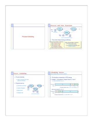
1. Processes and State Transitions
Ready
Ready Running
Running
Head
Tail
ready queue Waiting
Waiting
Head
Tail
Process Scheduling
resource/synchronization queues
Three states: Ready, Running, and Waiting
When aaprocess makes aatransition:
When process makes transition: Why aaprocess makes aatransition:
Why process makes transition:
1. from running to waiting
1. from running to waiting 1. an action of the process
1. an action of the process
2. from running to ready
2. from running to ready non-preemptive scheduling
non-preemptive scheduling
3. from waiting to ready
3. from waiting to ready 2. occurrence of an external event
2. occurrence of an external event
(3aa.aaprocess is created )) preemptive scheduling
(3 . process is created preemptive scheduling
4. from running to terminated
1 2
Scheduling Policies
Process Scheduling First-Come-First-Served (FCFS)
Process scheduling The discipline corresponding to FIFO queuing
ÿ Select a process from ready Example — 3 processes w/ compute times 12, 3, and 3
queue for execution ÿ Job arrival order P1, P2 , P3
Evaluation metrics
Execution P1
P1 P2
P2 P3
P3
ÿ CPU/device utilization Ready
Ready Running
Running Time 0 12 15 18
Average response time = ( 12 + 15 + 18 )/3 = 15
ÿ System throughput
ready Waiting
Waiting
queue
Job arrival order P2, P3, P1
ÿ Waiting time
Execution P2
P2 P3
P3 P1
P1
ÿ Response time Time 0 3 6 18
synchronization queues
Average response time = ( 3 + 6 + 18 ) /3 = 9
3 4
2. Scheduling Policies
FCFS Scheduling (Cont’d.) Shortest-Job-First (SJF)
Advantage: Select the shortest job first
ÿ Simple ÿ Enqueue jobs in order of estimated completion time
Disadvantages:
ÿ Average waiting time is highly variable
Head Pw, c = 9
v Short jobs may wait behind long ones !!
ÿ May lead to poor overlap between I/O and CPU processing Px, c = 12
Ready
Ready Running
Running
v CPU bound processes will make I/O bounds processes to wait fi
I/O devices remain idle
Py, c = 34
Tail Pz, c = 62 Waiting
Waiting
ready
queue
semaphore/condition queues
5 6
Shortest-Job-First Scheduling
An optimal policy for minimizing response times SJF Scheduling --- The Catch
Intuition: Consider an SJF execution of a set of processes It’s unfair !!
ÿ Continuous stream of short jobs will starve long jobs
Average response time = (r1 + r2 + r3 + r4 + r5 + r6)/6
SJF: P11 P22 P3 P4 P5 P6 Needs clairvoyance
P P P3 P4 P5 P6
0 r1 r2 r3 r4 r5 r6 ÿ Need to know the execution time of a process
ÿ Simple solution: ask the user !
Can switching the execution order reduce response time? ÿ Yeah, right !!
XYZ: P11 P22
P P P4
P4 P5
P5 P3
P3 P6
P6 So, what if you don’t subscribe to the Psychic Network ??
0 r1 r2 r4 – c3 r5 – c3 r3+c 4+c 5 r6
Average response
time = (r1 + r2 + r4–c3 + r5–c3 + r4+c4+c5 + r6)/6
= (r1 + r2 + r3 + r4 + r5 + r6 + (c4+c5–2c3))/6
7 8
3. Short-Job-First Scheduling Scheduling Policies
Estimating execution time Priority Scheduling (PS)
Jobs are enqueued in order of estimated completion time Assign a priority (a number) to each job and schedule jobs in
ÿ “Recent history is a good indicator of the near future” order of priority
ÿ Typically low priority values = “high priority”
E.g., if priority = tn, then a priority scheduler becomes a SJF
process P
process P scheduler.
begin
begin
loop
loop
<read input from user>
<process input>
<process input>
end loop
end loop
end P
Px Pc Pb Pa CPU
CPU
end P
Low High
t n — duration of the nth CPU burst Priority Priority
tn+1 — predicted duration of the n+1 st CPU burst (large (small
number) number)
tn+1 = atn + (1– a)tn, for 0 ≤ a ≤ 1
9 10
Priority Scheduling
Avoiding starvation Non Pre-emptive vs. Pre-emptive Scheduling
Aging Non Pre-emptive Scheduling:
ÿ Gradually increase a process’s priority (decrease its priority value) ÿ Once a process begins execution, it occupies CPU until it
over time finishes or it blocks
ÿ Advantage: simplicity, but …
ÿ Creates problems … (like what?)
Priority
ÿ Examples: FCFS, SJF, PS, …
Pre-emptive Scheduling:
Time ÿ A process is switched back and forth between running and
ready states
ÿ Advantage: more efficient, better capabilities, but …
ÿ More complex and needs hardware support (e.g., timer
Px Pc Pb Pa CPU interrupts)
CPU
ÿ Examples: Round Robin, Shortest Remaining Time First (SRTF),
Multi-level Feedback Queue (MLF)
11 12
4. Scheduling Policies
Round-Robin Scheduling (RR) RR Scheduling: Selecting a Time Quantum
Allocate the processor in discrete unit called quanta (or time- Too large
slices)
ÿ Long waiting time
ÿ Degenerates to FCFS in the limit
Switch to the next ready process at the end of each quantum
ÿ Processes execute every (n – 1) q time units
Too small
ÿ Responsive, but …
Process ÿ Throughput suffers due to large context switch overhead
<q Completion
Px Pc Pb Pa CPU
CPU or
I/O Request
Goal:
=q
ÿ Select a time quantum that balances this tradeoff
Timer Interrupt ÿ Rule of thumb: maintain context switch overhead to less
than 1%
13 14
Scheduling Policies
Multi-level feedback queues (MLF)
n priority levels — priority scheduling between levels, round-
robin within a level
Quantum size decreases with priority level
Jobs are demoted to lower priority levels if they don’t
complete within the current quantum
Level 1
q = t0
High
Priority Pa
Level 2
q = 2t0
P3 P2 P1
CPU
CPU
...
...
Level n
Low
Priority Py Px q = 2 n-1 t
0
15