Skills of SoftwareDeveloper
4
• The following are the ten skills to be possessed by a software
Developer
– Analytical ability
– Analysis
– Design
– Technical knowledge
– Programming ability
– Testing
– Quality planning and Practice
– Innovation
– Team working
– Communication
5.
Performance measures
5
• Thefollowing are the five points deciding the performance of a
software developer
– Timeliness
– Quality of work
– Customer Orientation
– Optimal solution
– Team satisfaction
6.
Problem-Definition
6
• Definition: Aproblem is a puzzle that requires logical thought or
mathematics to solve
• What is Problem solving ?
The act of defining a problem; determining its cause; identifying,
prioritizing and selecting alternatives for a solution; and implementing that
solution.
7.
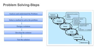
Problem Solving-Steps
Analyze andunderstand the Problem
Select a method to solve the problem
Design a solution
Develop the solution
Test the solution
7
8.
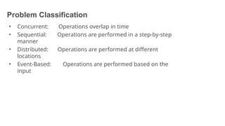
Problem Classification
8
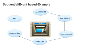
• Concurrent:Operations overlap in time
• Sequential: Operations are performed in a step-by-step
manner
• Distributed: Operations are performed at different
locations
• Event-Based: Operations are performed based on the
input
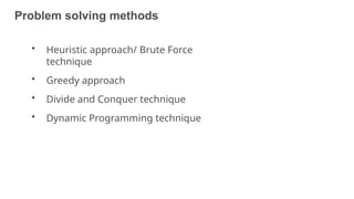
Problem solving methods
11
•Heuristic approach/ Brute Force
technique
• Greedy approach
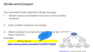
• Divide and Conquer technique
• Dynamic Programming technique
12.
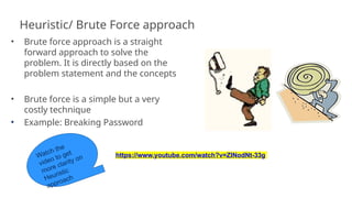
Heuristic/ Brute Forceapproach
• Brute force approach is a straight
forward approach to solve the
problem. It is directly based on the
problem statement and the concepts
• Brute force is a simple but a very
costly technique
• Example: Breaking Password
https://www.youtube.com/watch?v=ZINodNt-33g
12
13.
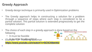
Greedy Approach
• Greedydesign technique is primarily used in Optimization problems
• The Greedy approach helps in constructing a solution for a problem
through a sequence of steps where each step is considered to be a
partial solution. This partial solution is extended progressively to get the
complete solution
• The choice of each step in a greedy approach is done based on the
following
– It must be feasible
– It must be locally optimal
– It must be irrevocable
• Example: TSP- Traveling Salesman
Problem
•
https://www.youtube.com/watch?v=SC5CX8drAtU
13
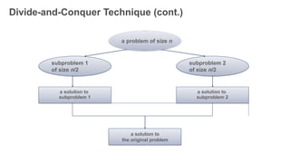
Divide-and-Conquer Technique (cont.)
subproblem2
of size n/2
subproblem 1
of size n/2
a solution to
the original problem
a solution to
subproblem 1
a solution to
subproblem 2
a problem of size n
15
16.
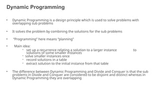
Dynamic Programming
16
• DynamicProgramming is a design principle which is used to solve problems with
overlapping sub problems
• It solves the problem by combining the solutions for the sub problems
• “Programming” here means “planning”
• Main idea:
- set up a recurrence relating a solution to a larger instance to
solutions of some smaller instances
- solve smaller instances once
- record solutions in a table
- extract solution to the initial instance from that table
• The difference between Dynamic Programming and Divide and Conquer is that the sub
problems in Divide and Conquer are considered to be disjoint and distinct whereas in
Dynamic Programming they are overlapping
17.
Dynamic Programming-Example
17
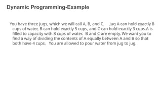
You havethree jugs, which we will call A, B, and C. Jug A can hold exactly 8
cups of water, B can hold exactly 5 cups, and C can hold exactly 3 cups.A is
filled to capacity with 8 cups of water. B and C are empty. We want you to
find a way of dividing the contents of A equally between A and B so that
both have 4 cups. You are allowed to pour water from jug to jug.
18.
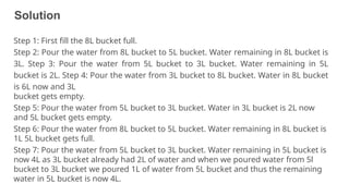
Solution
18
Step 1: Firstfill the 8L bucket full.
Step 2: Pour the water from 8L bucket to 5L bucket. Water remaining in 8L bucket is
3L. Step 3: Pour the water from 5L bucket to 3L bucket. Water remaining in 5L
bucket is 2L. Step 4: Pour the water from 3L bucket to 8L bucket. Water in 8L bucket
is 6L now and 3L
bucket gets empty.
Step 5: Pour the water from 5L bucket to 3L bucket. Water in 3L bucket is 2L now
and 5L bucket gets empty.
Step 6: Pour the water from 8L bucket to 5L bucket. Water remaining in 8L bucket is
1L 5L bucket gets full.
Step 7: Pour the water from 5L bucket to 3L bucket. Water remaining in 5L bucket is
now 4L as 3L bucket already had 2L of water and when we poured water from 5l
bucket to 3L bucket we poured 1L of water from 5L bucket and thus the remaining
water in 5L bucket is now 4L.
19.
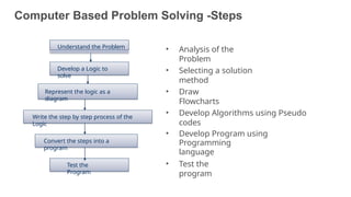
Computer Based ProblemSolving -Steps
• Analysis of the
Problem
• Selecting a solution
method
• Draw
Flowcharts
• Develop Algorithms using Pseudo
codes
• Develop Program using
Programming
language
• Test the
program
Understand the Problem
Develop a Logic to
solve
Represent the logic as a
diagram
Write the step by step process of the
Logic
Convert the steps into a
program
Test the
Program
19
20.
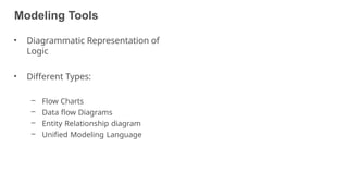
Modeling Tools
20
• DiagrammaticRepresentation of
Logic
• Different Types:
– Flow Charts
– Data flow Diagrams
– Entity Relationship diagram
– Unified Modeling Language
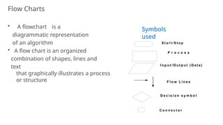
Flow Charts
• Aflowchart is a
diagrammatic representation
of an algorithm
• A flow chart is an organized
combination of shapes, lines and
text
that graphically illustrates a process
or structure
P r o c e s s
I n p u t / O u t p u t ( Da t a )
F l o w L i n e s
D e c i s i o n s y m b o l
C o n n e c t o r
S t a r t / S t o p
22
Symbols
used
23.
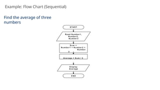
Example: Flow Chart(Sequential)
S TA R T
R e a d N u m b e r 1 ,
N u m b e r 2 ,
N u m b e r 3
S u m =
N u m b e r 1 + N u m b e r 2 +
N u m b e r
3
Av e r a g e = S u m / 3
D i sp l ay
Av e r a g e
E N D
Find the average of three
numbers
23
24.
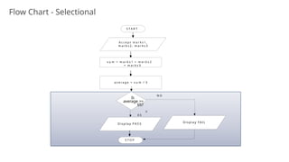
Flow Chart -Selectional
S T A R T
A c c e p t m a r k s 1 ,
m a r k s 2 , m a r k s 3
s u m = m a r k s 1 + m a r k s 2
+ m a r k s 3
a v e r a g e = s u m / 3
S T O P
N O
D i s p l a y P A S S
D i s p l a y FAI L
Is
average >=
65?
Y
E S
24
25.
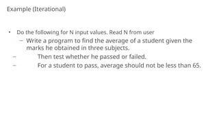
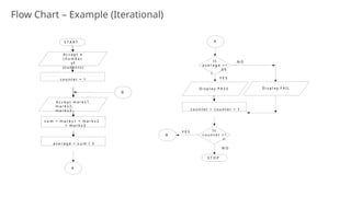
Example (Iterational)
25
• Dothe following for N input values. Read N from user
− Write a program to find the average of a student given the
marks he obtained in three subjects.
− Then test whether he passed or failed.
− For a student to pass, average should not be less than 65.
26.
Flow Chart –Example (Iterational)
S T A R T
A c c e p t m a r k s 1 ,
m a r k s 2 ,
m a r k s 3
s u m = m a r k s 1 + m a r k s 2
+ m a r k s 3
D i s p l a y P A S S
S T O P
a v e r a g e = s u m / 3
Is
a v e r a g e > =
6 5
?
N O
Y E S
A c c e p t n
( n u m b e r
o f
s t u d e n t s )
c o u n t e r = 1
D i s p l a y F A I L
c o u n t e r = c o u n t e r + 1
Is
c o u n t e r < =
n
N O
Y E S
A
A
B
B
26
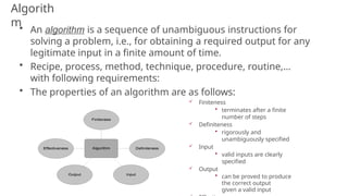
Algorith
m• An algorithmis a sequence of unambiguous instructions for
solving a problem, i.e., for obtaining a required output for any
legitimate input in a finite amount of time.
• Recipe, process, method, technique, procedure, routine,…
with following requirements:
• The properties of an algorithm are as follows:
Finiteness
• terminates after a finite
number of steps
Definiteness
• rigorously and
unambiguously specified
Input
• valid inputs are clearly
specified
Output
• can be proved to produce
the correct output
given a valid input 28
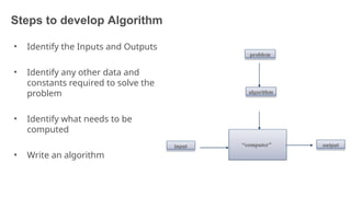
29.
Steps to developAlgorithm
• Identify the Inputs and Outputs
• Identify any other data and
constants required to solve the
problem
• Identify what needs to be
computed
• Write an algorithm
“computer”
problem
algorithm
input output
29
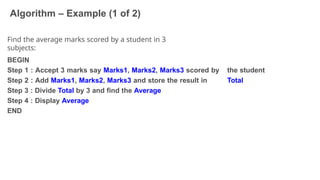
30.
Algorithm – Example(1 of 2)
30
Find the average marks scored by a student in 3
subjects:
the student
Total
BEGIN
Step 1 : Accept 3 marks say Marks1, Marks2, Marks3 scored by
Step 2 : Add Marks1, Marks2, Marks3 and store the result in
Step 3 : Divide Total by 3 and find the Average
Step 4 : Display Average
END
31.
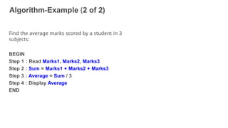
Algorithm-Example (2 of2)
31
Find the average marks scored by a student in 3
subjects:
BEGIN
Step 1 : Read Marks1, Marks2, Marks3
Step 2 : Sum = Marks1 + Marks2 + Marks3
Step 3 : Average = Sum / 3
Step 4 : Display Average
END
32.
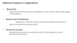
Different Patterns inAlgorithms
32
• Sequential
– Sequential constructs execute the program in the order in which they appear
in the program
• Selectional (Conditional)
– Selectional constructs control the flow of statement execution in
order to achieve the required result
• Iterational (Loops)
– Iterational constructs are used when a part of the program is to be
executed several times
33.
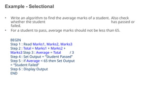
Example - Selectional
33
•Write an algorithm to find the average marks of a student. Also check
whether the student has passed or
failed.
• For a student to pass, average marks should not be less than 65.
BEGIN
Step 1 : Read Marks1, Marks2, Marks3
Step 2 : Total = Marks1 + Marks2 +
Marks3 Step 3 : Average = Total / 3
Step 4 : Set Output = “Student Passed”
Step 5 : if Average < 65 then Set Output
= “Student Failed”
Step 6 : Display Output
END
34.
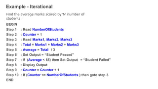
Example - Iterational
34
Findthe average marks scored by ‘N’ number of
students
BEGIN
Step 1
Step 2
Step 3
Step 4
Step 5
Step 6
Step 7
Step 8
Step 9
: Read NumberOfStudents
: Counter = 1
: Read Marks1, Marks2, Marks3
: Total = Marks1 + Marks2 + Marks3
: Average = Total / 3
: Set Output = “Student Passed”
: If (Average < 65) then Set Output = “Student Failed”
: Display Output
: Counter = Counter + 1
Step 10 : If (Counter <= NumberOfStudents ) then goto step 3
END
35.
Recap
• Skills ofa software
developer
• Problem classification
• Problem solving
approaches
• Flow Chart
• Algorithm patterns
Data Structures
37
• Datastructures is concerned with the representation and manipulation
of data
• All programs manipulate data
• So, all programs represent data in some way
• Data manipulation requires an algorithm
• The study of Data Structure is fundamental to computer programming
38.
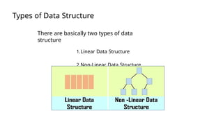
Types of DataStructure
There are basically two types of data
structure
1.Linear Data Structure
2.Non-Linear Data Structure.
38
39.
Basic data structures:data collections
39
• Linear structures
– Array: Fixed-size
– Linked List: Add to top, bottom or in the middle
– Stack: Add to top and remove from top
– Queue: Add to back and remove from front
– Priority queue: Add anywhere, remove the highest
priority
• Non- Linear Data Structure
– Tree: A branching structure with no loops
– Graph: A more general branching structure, with
less
stringent connection conditions than for a tree
40.
Static vs. DynamicStructures
• A static data structure has a fixed size
This meaning is different from the meaning of the static modifier
(variable
shared among all instances of a class)
• Arrays are static; once you define the number of elements it can
hold, the number doesn’t change
• A dynamic data structure grows and shrinks at execution time as
required by its contents
• A dynamic data structure is implemented using links
40
41.
Array
[0] [1] [2][3] [4] [5] [6] [7]
0 0 0 0 0 0 0 0
Age
0 0 0 38 0 0 0 0
[0] [1] [2] [3] [4] [5] [6] [7]
Age
1
int [ ] Age;
Declaratio
n
2 Age= new int[8];
Allocatio
n
3 Age [3] = 38;
Initialization
Age
41
(Arrays are like objects)
An array of
integers
42.
Linked List
42
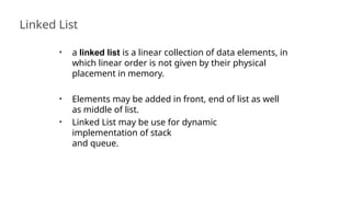
• alinked list is a linear collection of data elements, in
which linear order is not given by their physical
placement in memory.
• Elements may be added in front, end of list as well
as middle of list.
• Linked List may be use for dynamic
implementation of stack
and queue.
43.
Stack
43
• Stack isa linear data structure which works on
LIFO order. So that Last In First Out .
• In stack element is always added at top of stack
and also removed from top of the stack.
• Stack is useful in recursive function, function
calling, mathematical expression calculation,
reversing the string etc.
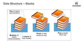
44.
Data Structure --Stacks
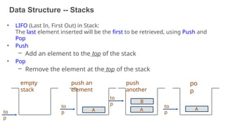
• LIFO (Last In, First Out) in Stack:
The last element inserted will be the first to be retrieved, using Push and
Pop
• Push
– Add an element to the top of the stack
• Pop
– Remove the element at the top of the stack
to
p
empty
stack
A
to
p
push an
element
to
p
push
another
A
B
to
p
po
p
44
A
45.
Data Structures --Stacks
45
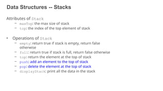
Attributes of Stack
– maxTop: the max size of stack
– top: the index of the top element of stack
• Operations of Stack
– empty: return true if stack is empty, return false
otherwise
– full: return true if stack is full, return false otherwise
– top: return the element at the top of stack
– push: add an element to the top of stack
– pop: delete the element at the top of stack
– displayStack: print all the data in the stack
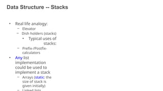
46.
Data Structure --Stacks
46
• Real life analogy:
– Elevator
– Dish holders (stacks)
• Typical uses of
stacks:
– Prefix-/Postfix-
calculators
• Any list
implementation
could be used to
implement a stack
– Arrays (static: the
size of stack is
given initially)
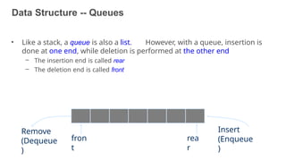
Data Structure --Queues
• Like a stack, a queue is also a list. However, with a queue, insertion is
done at one end, while deletion is performed at the other end
– The insertion end is called rear
– The deletion end is called front
Insert
(Enqueue
)
Remove
(Dequeue
)
rea
r
fron
t
48
49.
Data Structure --Queues
49
• Attributes of Queue
– front/rear: front/rear index
– counter: number of elements in the queue
– maxSize: capacity of the queue
• Operations of Queue
– IsEmpty: return true if queue is empty, return false
otherwise
– IsFull: return true if queue is full, return false otherwise
– Enqueue: add an element to the rear of queue
– Dequeue: delete the element at the front of queue
– DisplayQueue: print all the data
50.
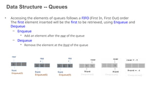
Data Structure --Queues
• Accessing the elements of queues follows a FIFO (First In, First Out) order
The first element inserted will be the first to be retrieved, using Enqueue and
Dequeue
– Enqueue
• Add an element after the rear of the queue
– Dequeue
• Remove the element at the front of the queue
rear
front
Enqueue(3)
3
rea
r
front
Enqueue(6)
3 6
rea
r
front
Enqueue(9)
3 6 9
50
51.
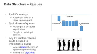
Data Structure --Queues
• Real life analogy:
– Check-out lines in a
store (queuing up)
• Typical uses of queues:
– Waiting lists of course
registration
– Simple scheduling in
routers
• Any list implementation
could be used to
implement a queue
– Arrays (static: the size of
queue is given initially)
– Linked lists (dynamic: 51


![Array
[0] [1] [2] [3] [4] [5] [6] [7]
0 0 0 0 0 0 0 0
Age
0 0 0 38 0 0 0 0
[0] [1] [2] [3] [4] [5] [6] [7]
Age
1
int [ ] Age;
Declaratio
n
2 Age= new int[8];
Allocatio
n
3 Age [3] = 38;
Initialization
Age
41
(Arrays are like objects)
An array of
integers](https://image.slidesharecdn.com/1-250507084952-90ba92f2/85/1-Problem-Solving-Techniques-and-Data-Structures-pptx-41-320.jpg)