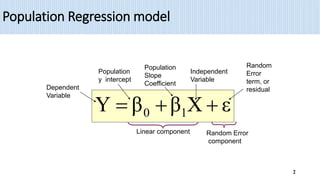
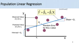
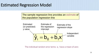
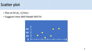
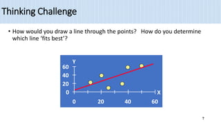
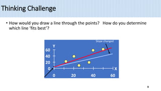
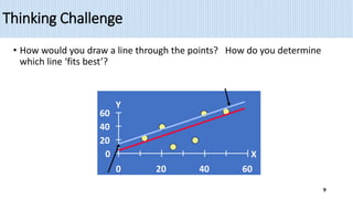
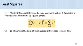
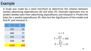
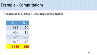
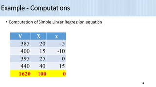
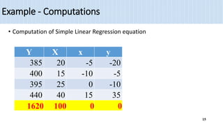
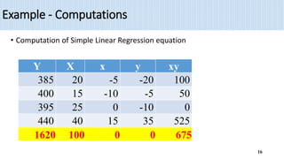
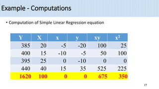
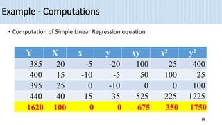
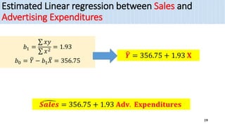
1) Simple linear regression models the relationship between a dependent variable (Y) and a single independent variable (X) as a linear equation. It finds the line of best fit to the data and uses this to estimate or predict future values of Y based on X. 2) The document provides an example of using simple linear regression to model the relationship between weekly sales (Y) and advertising expenditures (X) for a retail merchant. It estimates the regression equation and uses this to predict sales for a given expenditure level. 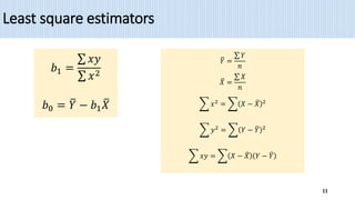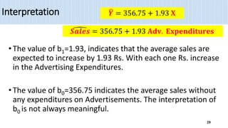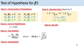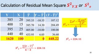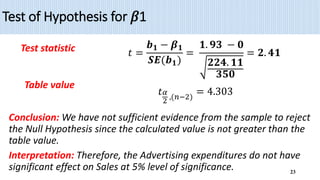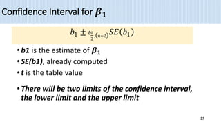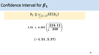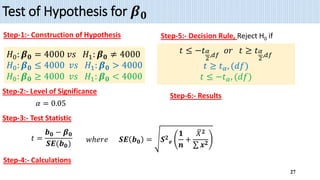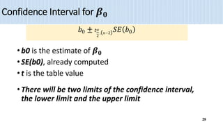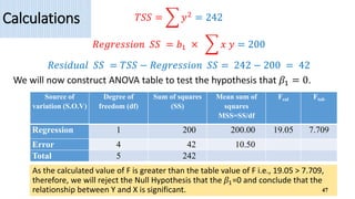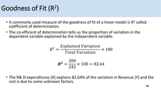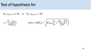3) Key outputs of the simple linear regression analysis are presented, including estimating the regression coefficients, testing their significance, calculating confidence intervals and analyzing the variance (ANOVA).

1. Simple Linear Regression
1

2. ε
X
β
β
Y 1
0 


Linear component
Population Regression model
Population
y intercept
Population
Slope
Coefficient
Random
Error
term, or
residual
Dependent
Variable
Independent
Variable
Random Error
component
2

3. Linear Regression Assumptions
• Error values (ε) are statistically independent
• Error values are normally distributed for any given value of x
• The probability distribution of the errors is normal
• The probability distribution of the errors has constant variance
• The underlying relationship between the x variable and the y
variable is linear
3

4. Population Linear Regression
(continued)
Random Error
for this x value
y
x
Observed Value
of y for xi
Predicted Value
of y for xi
X
β̂
β̂
ˆ
1
0 

Y
xi
Slope = β1
Intercept = β0
εi
4

5. x
b
b
ŷ 1
0
i 

The sample regression line provides an estimate of
the population regression line
Estimated Regression Model
Estimate of
the regression
intercept
Estimate of the
regression slope
Estimated
(or predicted)
y value
Independent
variable
The individual random error terms ei have a mean of zero
5

6. Scatter plot
• Plot of All (Xi, Yi) Pairs
• Suggests How Well Model Will Fit
0
20
40
60
0 20 40 60
X
Y
6

7. Thinking Challenge
• How would you draw a line through the points? How do you determine
which line ‘fits best’?
0
20
40
60
0 20 40 60
X
Y
7

8. Thinking Challenge
• How would you draw a line through the points? How do you determine
which line ‘fits best’?
0
20
40
60
0 20 40 60
X
Y
Slope changed
Intercept unchanged
8

9. Thinking Challenge
• How would you draw a line through the points? How do you determine
which line ‘fits best’?
Slope changed
0
20
40
60
0 20 40 60
X
Y
Intercept changed
9

10. Least Squares
• 1. ‘Best Fit’ Means Difference Between Actual Y Values & Predicted Y
Values Are a Minimum. So square errors!
• 2. LS Minimizes the Sum of the Squared Differences (errors) (SSE)
  
 



n
i
i
n
i
i
i Y
Y
1
2
1
2
ˆ
ˆ 
10

11. Least square estimators
11
𝑏1 =
𝑥𝑦
𝑥2
𝑏0 = 𝑌 − 𝑏1𝑋
𝑌 =
𝑌
𝑛
𝑋 =
𝑋
𝑛
𝑥2 = 𝑋 − 𝑋 2
𝑦2
= 𝑌 − 𝑌 2
𝑥𝑦 = 𝑋 − 𝑋 𝑌 − 𝑌

12. Example
A study was made by a retail merchant to determine the relation between
weekly advertising expenditures (X) and sales (Y). Estimate regression line to
predict weekly sales from advertising expenditures and interpret it. Predict the
Sales for a weekly expenditures 29. Also test the Significance of the model and
find R2 and interpret it.
12
Y X
385 20
400 15
395 25
440 40
𝑛 = 4
𝑌 =
𝑌
𝑛
= 405
𝑋 =
𝑋
𝑛
= 25
1620 100

13. Example - Computations
• Computation of Simple Linear Regression equation
13
Y X
385 20
400 15
395 25
440 40
1620 100

14. Example - Computations
• Computation of Simple Linear Regression equation
14
Y X x
385 20 -5
400 15 -10
395 25 0
440 40 15
1620 100 0

15. Example - Computations
• Computation of Simple Linear Regression equation
15
Y X x y
385 20 -5 -20
400 15 -10 -5
395 25 0 -10
440 40 15 35
1620 100 0 0

16. Example - Computations
• Computation of Simple Linear Regression equation
16
Y X x y xy
385 20 -5 -20 100
400 15 -10 -5 50
395 25 0 -10 0
440 40 15 35 525
1620 100 0 0 675

17. Example - Computations
• Computation of Simple Linear Regression equation
17
Y X x y xy x2
385 20 -5 -20 100 25
400 15 -10 -5 50 100
395 25 0 -10 0 0
440 40 15 35 525 225
1620 100 0 0 675 350

18. Example - Computations
• Computation of Simple Linear Regression equation
18
Y X x y xy x2 y2
385 20 -5 -20 100 25 400
400 15 -10 -5 50 100 25
395 25 0 -10 0 0 100
440 40 15 35 525 225 1225
1620 100 0 0 675 350 1750

19. Estimated Linear regression between Sales and
Advertising Expenditures
𝑺𝒂𝒍𝒆𝒔 = 356.75 + 1.93 𝐀𝐝𝐯. 𝐄𝐱𝐩𝐞𝐧𝐝𝐢𝐭𝐮𝐫𝐞𝐬
19
𝑏1 =
𝑥𝑦
𝑥2
= 1.93
𝑏0 = 𝑌 − 𝑏1𝑋 = 356.75
𝒀 = 356.75 + 1.93 𝐗

20. Interpretation
20
•The value of b1=1.93, indicates that the average sales are
expected to increase by 1.93 Rs. With each one Rs. increase
in the Advertising Expenditures.
•The value of b0=356.75 indicates the average sales without
any expenditures on Advertisements. The interpretation of
b0 is not always meaningful.
𝑺𝒂𝒍𝒆𝒔 = 356.75 + 1.93 𝐀𝐝𝐯. 𝐄𝐱𝐩𝐞𝐧𝐝𝐢𝐭𝐮𝐫𝐞𝐬
𝒀 = 356.75 + 1.93 𝐗

21. Test of Hypothesis for 𝛽1
Step-1:- Construction of Hypothesis
Step-2:- Level of Significance
Step-3:- Test Statistic
Step-4:- Calculations
Step-5:- Decision Rule, Reject H0 if
Step-6:- Results
21
𝑤ℎ𝑒𝑟𝑒 𝑺𝑬 𝒃𝟏 =
𝑺𝟐
𝒆
𝒙𝟐
𝑡 =
𝒃𝟏 − 𝜷𝟏
𝑺𝑬(𝒃𝟏)
𝛼 = 0.05
𝐻0: 𝜷𝟏 = 0 𝑣𝑠 𝐻1: 𝜷𝟏 ≠ 0
𝐻0: 𝜷𝟏 ≤ 0 𝑣𝑠 𝐻1: 𝜷𝟏 > 0
𝐻0: 𝜷𝟏 ≥ 0 𝑣𝑠 𝐻1: 𝜷𝟏 < 0
𝑡 ≤ −𝑡𝛼
2,𝑑𝑓
𝑜𝑟 𝑡 ≥ 𝑡𝛼
2,𝑑𝑓
𝑡 ≥ 𝑡𝛼, (𝑑𝑓)
𝑡 ≤ −𝑡𝛼, (𝑑𝑓)

22. Calculation of Residual Mean Square 𝑺𝟐
𝒀.𝑿 or 𝑺𝟐
𝒆
22
𝑺𝟐
𝒆 =
𝒀 − 𝑌
𝟐
𝒏 − 𝟐
= 𝟐𝟐𝟒. 𝟏𝟏
𝑺𝟐
𝒆 =
𝒚𝟐 −
𝒙𝒚 𝟐
𝒙𝟐
𝒏 − 𝟐
𝑺𝟐
𝒆 = 𝟐𝟐𝟒. 𝟏𝟏
Y X
385 20
400 15
395 25
440 40
1620 100
𝒀
395.35
385.70
405.00
433.95
𝒀 − 𝒀
-10.35
14.30
-10.00
6.05
0
(Y - 𝒀)2
107.12
204.49
100.00
36.60
448.22

23. Test of Hypothesis for 𝛽1
23
𝑡 =
𝒃𝟏 − 𝜷𝟏
𝑺𝑬(𝒃𝟏)
=
𝟏. 𝟗𝟑 − 𝟎
𝟐𝟐𝟒. 𝟏𝟏
𝟑𝟓𝟎
= 𝟐. 𝟒𝟏
Table value
𝑡𝛼
2
,(𝑛−2)
= 4.303
Test statistic
Conclusion: We have not sufficient evidence from the sample to reject
the Null Hypothesis since the calculated value is not greater than the
table value.
Interpretation: Therefore, the Advertising expenditures do not have
significant effect on Sales at 5% level of significance.

24. PERCENTAGE POINT OF STUDENT'S t-DISTRIBUTION
d.f.
Alpha
0.250 0.100 0.050 0.025 0.0125 0.005
1 1.000 3.078 6.314 12.706 31.821 63.657
2 0.816 1.886 2.920 4.303 6.965 9.925
3 0.765 1.638 2.353 3.182 4.541 5.841
4 0.741 1.533 2.132 2.776 3.747 4.604
5 0.727 1.476 2.015 2.571 3.365 4.032
6 0.718 1.440 1.943 2.447 3.143 3.707
7 0.711 1.415 1.895 2.365 2.998 3.499
8 0.706 1.397 1.860 2.306 2.896 3.355
9 0.703 1.383 1.833 2.262 2.821 3.250
10 0.700 1.372 1.812 2.228 2.764 3.169
11 0.697 1.363 1.796 2.201 2.718 3.106
12 0.695 1.356 1.782 2.179 2.681 3.055
13 0.694 1.350 1.771 2.160 2.650 3.012
14 0.692 1.345 1.761 2.145 2.624 2.977
15 0.691 1.341 1.753 2.131 2.602 2.947
16 0.690 1.337 1.746 2.120 2.583 2.921
17 0.689 1.333 1.740 2.110 2.567 2.898
18 0.688 1.330 1.734 2.101 2.552 2.878
24

25. Confidence Interval for 𝜷𝟏
• b1 is the estimate of 𝜷𝟏
• SE(b1), already computed
• t is the table value
• There will be two limits of the confidence interval,
the lower limit and the upper limit
25
𝑏1 ± 𝑡𝛼
2
,(𝑛−2)𝑆𝐸(𝑏1)

26. Confidence Interval for 𝜷𝟏
26
𝟏. 𝟗𝟑 ± 𝟒. 𝟑𝟎𝟑
𝟐𝟐𝟒. 𝟏𝟏
𝟑𝟓𝟎
−𝟏. 𝟓𝟏 , 𝟓. 𝟑𝟕
𝑏1 ± 𝑡𝛼
2
,(𝑛−2)𝑆𝐸(𝑏1)

27. Test of Hypothesis for 𝜷𝟎
Step-1:- Construction of Hypothesis
Step-2:- Level of Significance
Step-3:- Test Statistic
Step-4:- Calculations
Step-5:- Decision Rule, Reject H0 if
Step-6:- Results
27
𝑤ℎ𝑒𝑟𝑒 𝑺𝑬 𝒃𝟎 = 𝑺𝟐
𝒆
𝟏
𝒏
+
𝑋𝟐
𝒙𝟐
𝑡 =
𝒃𝟎 − 𝜷𝟎
𝑺𝑬(𝒃𝟎)
𝛼 = 0.05
𝐻0: 𝜷𝟎 = 4000 𝑣𝑠 𝐻1: 𝜷𝟎 ≠ 4000
𝐻0: 𝜷𝟎 ≤ 4000 𝑣𝑠 𝐻1: 𝜷𝟎 > 4000
𝐻0: 𝜷𝟎 ≥ 4000 𝑣𝑠 𝐻1: 𝜷𝟎 < 4000
𝑡 ≤ −𝑡𝛼
2,𝑑𝑓
𝑜𝑟 𝑡 ≥ 𝑡𝛼
2,𝑑𝑓
𝑡 ≥ 𝑡𝛼, (𝑑𝑓)
𝑡 ≤ −𝑡𝛼, (𝑑𝑓)

28. Confidence Interval for 𝜷𝟎
• b0 is the estimate of 𝜷𝟎
• SE(b0), already computed
• t is the table value
• There will be two limits of the confidence interval,
the lower limit and the upper limit
28
𝑏0 ± 𝑡𝛼
2
,(𝑛−2)𝑆𝐸(𝑏0)

29. ANOVA
• Partition of total variation in Response Variable Y into two components i.e.,
explained (due to Regression) and the unexplained (Residual) variation. Explained
variation is the variation due to regression i.e., variation due to X and the
unexplained variation is the variation due to uncontrolled factors other than X.
TSS = Regression SS + Residual SS
𝑇𝑆𝑆 = 𝑦2
𝑅𝑒𝑔𝑟𝑒𝑠𝑠𝑖𝑜𝑛 𝑆𝑆 = 𝑏1 × 𝑥 𝑦
𝑅𝑒𝑠𝑖𝑑𝑢𝑎𝑙 𝑆𝑆 = 𝑇𝑆𝑆 − 𝑅𝑒𝑔𝑟𝑒𝑠𝑠𝑖𝑜𝑛 𝑆𝑆
29

30. Calculations 𝑇𝑆𝑆 = 𝑦2 = 1750
𝑅𝑒𝑔𝑟𝑒𝑠𝑠𝑖𝑜𝑛 𝑆𝑆 = 𝑏1 × 𝑥 𝑦 = 1301.79
𝑅𝑒𝑠𝑖𝑑𝑢𝑎𝑙 = 𝑇𝑆𝑆 − 𝑅𝑒𝑔𝑟𝑒𝑠𝑠𝑖𝑜𝑛 𝑆𝑆 = 448.21
We will now construct ANOVA table to test the hypothesis that 𝛽1 = 0.
Source of
variation
(S.O.V)
Degree of
freedom (df)
Sum of squares
(SS)
Mean sum of
squares
MSS=SS/df
Fcal Ftab
Regression 1 1301.79 1301.79 5.80 18 . 513
Residual 2 448.21 224.11
Total 3 1750
As the calculated value of F is not greater than the table value, therefore, we
have not sufficient evidence against the Null Hypothesis and conclude that
the Sales have not been affected significantly from Adv. Expenditures. 30

31. Goodness of Fit (R2)
• A commonly used measure of the goodness of fit of a linear model is R2 called
coefficient of determination.
• The co-efficient of determination tells us the proportion of variation in the
response variable explained by the independent variable.
𝑅2
=
𝐸𝑥𝑝𝑙𝑎𝑖𝑛𝑒𝑑 𝑉𝑎𝑟𝑖𝑎𝑡𝑖𝑜𝑛
𝑇𝑜𝑡𝑎𝑙 𝑉𝑎𝑟𝑖𝑎𝑡𝑖𝑜𝑛
× 100
𝑹𝟐
=
1301.79
1750
× 100 = 74.39%
• The Advertisement Expenditures (X) explains 74.39% of the variation in Sales (Y)
and the rest is due to some unknown factors.
31

32. Example
Following data shows the Revenue of six firms in (000)$ along with the
expenditures on Research & Development (000)$.
• Draw a scatter plot and assess the relationship between Y and X.
• Fit simple linear regression equation and interpret the parameters.
• Test the hypothesis that there is no linear relation between Y and X i.e., β1=0. Also
compute 95% Confidence Interval for β1.
• Test the hypothesis that β0 > 15. Compute 95% Confidence Interval for β0.
• Perform analysis of variance (ANOVA) and test the significance of the regression
model. Calculate coefficient of determination and interpret it.
• Test the hypothesis that the mean revenue for firm at X=9 is greater than 30 i.e.,
𝜇𝑌
𝑋=9
> 30. Also construct 95% Confidence Interval.
Revenue in (000) $ Y 31 40 30 34 25 20
Expenditure on R & D in (000) $ X 5 11 4 5 3 2
32

33. Interpretation
• The value of b1=2, indicates that the average yield of rice is expected to
increase by 2 maunds with each one kg increase in the fertilizer.
• The value of b0=20 indicates that average yield of rice will be 20 kg without
using the fertilizer. The interpretation of b0 is not always meaningful.
𝒀 = 20 + 2 𝑿
Muhammad Usman 38

34. ANOVA
• Partition of total variation in Response Variable Y into two components i.e.,
explained (due to Regression) and the unexplained (Residual) variation. Explained
variation is the variation due to regression i.e., variation due to X and the
unexplained variation is the variation due to uncontrolled factors other than X.
TSS = Regression SS + Residual SS
𝑇𝑆𝑆 = 𝑦2
𝑅𝑒𝑔𝑟𝑒𝑠𝑠𝑖𝑜𝑛 𝑆𝑆 = 𝑏1 × 𝑥 𝑦
𝑅𝑒𝑠𝑖𝑑𝑢𝑎𝑙 𝑆𝑆 = 𝑇𝑆𝑆 − 𝑅𝑒𝑔𝑟𝑒𝑠𝑠𝑖𝑜𝑛 𝑆𝑆
46

35. Calculations 𝑇𝑆𝑆 = 𝑦2 = 242
𝑅𝑒𝑔𝑟𝑒𝑠𝑠𝑖𝑜𝑛 𝑆𝑆 = 𝑏1 × 𝑥 𝑦 = 200
𝑅𝑒𝑠𝑖𝑑𝑢𝑎𝑙 𝑆𝑆 = 𝑇𝑆𝑆 − 𝑅𝑒𝑔𝑟𝑒𝑠𝑠𝑖𝑜𝑛 𝑆𝑆 = 242 − 200 = 42
We will now construct ANOVA table to test the hypothesis that 𝛽1 = 0.
Source of
variation (S.O.V)
Degree of
freedom (df)
Sum of squares
(SS)
Mean sum of
squares
MSS=SS/df
Fcal Ftab
Regression 1 200 200.00 19.05 7.709
Error 4 42 10.50
Total 5 242
As the calculated value of F is greater than the table value of F i.e., 19.05 > 7.709,
therefore, we will reject the Null Hypothesis that the 𝛽1=0 and conclude that the
relationship between Y and X is significant. 47

36. Goodness of Fit (R2)
• A commonly used measure of the goodness of fit of a linear model is R2 called
coefficient of determination.
• The co-efficient of determination tells us the proportion of variation in the
dependent variable explained by the independent variable.
𝑅2
=
𝐸𝑥𝑝𝑙𝑎𝑖𝑛𝑒𝑑 𝑉𝑎𝑟𝑖𝑎𝑡𝑖𝑜𝑛
𝑇𝑜𝑡𝑎𝑙 𝑉𝑎𝑟𝑖𝑎𝑡𝑖𝑜𝑛
× 100
𝑹𝟐
=
200
242
× 100 = 82.64
• The R& D expenditures (X) explains 82.64% of the variation in Revenue (Y) and the
rest is due to some unknown factors.
48

37. Test of hypothesis for
49
𝐻0: 𝜇𝑦/𝑥=9 ≤ 30 𝑣𝑠 𝐻1: 𝜇𝑦/𝑥=9 > 30
𝑡 =
𝑌𝑥 − 𝜇𝑦 𝑥
𝑆𝐸 𝑌𝑥
, 𝑤ℎ𝑒𝑟𝑒 SE 𝑌𝑥 = 𝑺𝟐
𝒀.𝑿
1
𝑛
+
𝑋0 − 𝑋 2
𝒙𝟐

38. Thanks
50