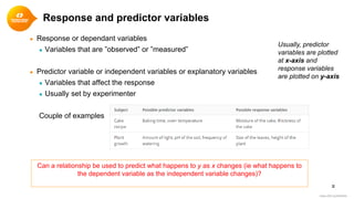
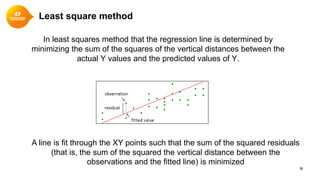
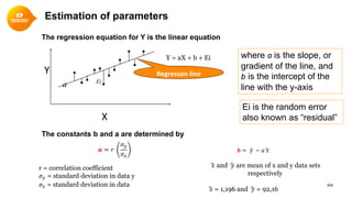
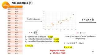
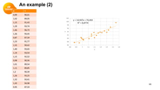
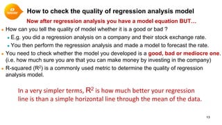
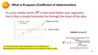
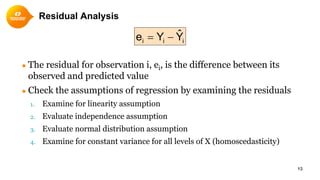
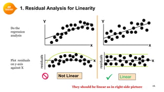
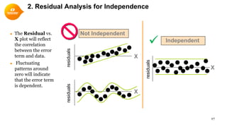
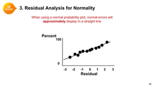
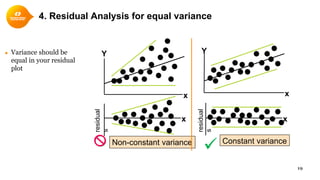
Lecture:
Simple Linear Regression
Chaudhary Awais Salman
Doctoral Researcher in Future Energy
Course instructor
School of Business, Society and Engineering
Fuuture Energy – Centre of Excellence
Email: Chaudhary.awais.salman@mdh.se
Response and predictor variables
● Response or dependant variables
● Variables that are ”observed” or ”measured”
● Predictor variable or independent variables or explanatory variables
● Variables that affect the response
● Usually set by experimenter
Couple of examples
2
https://bit.ly/2MZOIdv
Usually, predictor
variables are plotted
at x-axis and
response variables
are plotted on y-axis
Can a relationship be used to predict what happens to y as x changes (ie what happens to
the dependent variable as the independent variable changes)?
What is regression? (1)
● How do we predict one variable from another?
● How does one variable (Y) change as the other
changes (X)?
● Influence of one variable on another
3
“Regression analysis allows us to quantify the relationship between a
particular variable and an outcome that we care about while controlling
for other factors.”
Wheelan Charles, Naked Statistics
● Regression analysis is not used to obtain the “deterministic or exact” equation that
describes Y and X.
● Deterministic relationships are sometimes (although very rarely) used in business
environments.
assets=liabilities + owner equity
total costs=fixed costs + variable costs
● But in engineering and sciences rarely we get the deterministic or exact equations. There is
always a room for “error”
● Regression equation is used for modelling, predicting or forecasting.
4
What is regression? (2)
Regression Modeling Steps
• Hypothesize deterministic component
• Estimate unknown model parameters
• Specify probability distribution of random error term
• Estimate standard deviation of error
• Evaluate model
• Use model for prediction and estimation
5
Simple Linear regression
● Lets assume you have bivariate data (x1, y1), (x2, y2), (x3, y3), ……………..,(xn, yn)
● x is independent/predictor variable
● y is dependant/response variable
● Linear regression model (equation) would be
Y = aX + b + Ei
a = slope of straight line
b = y-intercept
Ei = error 
Goal of simple linear regression is to find the values of ”a” and ”b” that give the best fitting line.
Best fit will have the values of ”a” and ”b” that have minimum error, Ei
6
7
Simple Linear regression (2)
The regression equation for Y is the linear equation
.
. ..
. .
X
Regresson lineY
Y = aX + b + Ei where a is the slope, or
gradient of the line, and
b is the intercept of the
line with the y-axis
Ei is the random error
also known as “residual”
a Ei
Residuals
● When we predict Ŷ for a given X, we will sometimes be
in error.
● Y – Ŷ for any X is a an error of estimate also known as
a residual
● We want to Σ(Y- Ŷ) be as small as possible.
● BUT, there are infinitely many lines that can do this.
● Draw ANY line that goes through the mean of the X and
Y values.
● Minimize Errors of Estimate… How?
● By using “Least square method”
8
12108642
Y
30
20
10
0
Residual
Prediction
X,Ŷ
X,Y
• The method of least squares finds the straight line which minimises the sum of the
squared vertical deviations from the fitted line
• The best fitting line is called the least squares linear regression line
Least square method
In least squares method that the regression line is determined by
minimizing the sum of the squares of the vertical distances between the
actual Y values and the predicted values of Y.
9
A line is fit through the XY points such that the sum of the squared residuals
(that is, the sum of the squared the vertical distance between the
observations and the fitted line) is minimized
10
The regression equation for Y is the linear equation
The constants b and a are determined by
.
. ..
. .
X
Regresson lineY
𝒂𝒂 = 𝑟𝑟
𝜎𝜎𝑦𝑦
𝜎𝜎𝑥𝑥
Y = aX + b + Ei
r = correlation coefficient
𝜎𝜎𝑦𝑦 = standard deviation in data y
𝜎𝜎𝑥𝑥 = standard deviation in data
𝒃𝒃 = �𝑦𝑦 − 𝑎𝑎�𝑥𝑥
�𝑥𝑥 and �𝑦𝑦 are mean of x and y data sets
respectively
�𝑥𝑥 = 1,196 and �𝑦𝑦 = 92,16
where a is the slope, or
gradient of the line, and
b is the intercept of the
line with the y-axis
Ei is the random error
also known as “residual”
Estimation of parameters
a Ei
An example (1)
11
X Y
0,99 90,01
1,02 89,05
1,15 91,43
1,29 93,74
1,46 96,73
1,36 94,45
0,87 87,59
1,23 91,77
1,55 99,42
1,40 93,65
1,19 93,54
1,15 92,52
0,98 90,56
1,01 89,54
1,11 89,85
1,2 90,39
1,26 93,25
1,32 93,41
1,43 94,98
0,95 87,33
86
88
90
92
94
96
98
100
102
0,8 0,9 1 1,1 1,2 1,3 1,4 1,5 1,6
y
x
Scatter diagram
Y = aX + b
𝒂𝒂 = 𝑟𝑟
𝜎𝜎𝑦𝑦
𝜎𝜎𝑥𝑥
r = correlation coefficient = 0,936
𝜎𝜎𝑦𝑦 = standard deviation in data y = 2,944
𝜎𝜎𝑥𝑥 = standard deviation in data x = 0,184
a = 14,94
𝒃𝒃 = �𝒚𝒚 − 𝑎𝑎 ̅𝑥𝑥
̅𝑥𝑥and �𝒚𝒚 are mean of x and y data sets
respectively
̅𝑥𝑥 = 1,196 and �𝒚𝒚 = 92,16
b = 74,28
Regression model
y = 14,94x + 74,28
12
X Y
0,99 90,01
1,02 89,05
1,15 91,43
1,29 93,74
1,46 96,73
1,36 94,45
0,87 87,59
1,23 91,77
1,55 99,42
1,40 93,65
1,19 93,54
1,15 92,52
0,98 90,56
1,01 89,54
1,11 89,85
1,2 90,39
1,26 93,25
1,32 93,41
1,43 94,98
0,95 87,33
y = 14,947x + 74,283
R² = 0,8774
86
88
90
92
94
96
98
100
102
0,8 0,9 1 1,1 1,2 1,3 1,4 1,5 1,6
y
x
An example (2)
How to check the quality of regression analysis model
Now after regression analysis you have a model equation BUT…
● How can you tell the quality of model whether it is a good or bad ?
● E.g. you did a regression analysis on a company and their stock exchange rate.
● You then perform the regression analysis and made a model to forecast the rate.
● You need to check whether the model you developed is a good, bad or mediocre one.
(i.e. how much sure you are that you can make money by investing in the company)
● R-squared (R2) is a commonly used metric to determine the quality of regression
analysis model.
13
In a very simpler terms, R2 is how much better your regression
line is than a simple horizontal line through the mean of the data.
What is R-square (Coefficient of determination)
14
In a very simpler terms, R2 is how much better your regression
line is than a simple horizontal line through the mean of the data.
y = 14,947x + 74,283
R² = 0,8774
86
88
90
92
94
96
98
100
102
0,8 0,9 1 1,1 1,2 1,3 1,4 1,5 1,6
y
x
Mean of data
Regression line
FORMULA for R2
A convenient way of determining the R2 or coefficient of
determination is by taking the square of correlation of both x and y
Residual Analysis
● The residual for observation i, ei, is the difference between its
observed and predicted value
● Check the assumptions of regression by examining the residuals
1. Examine for linearity assumption
2. Evaluate independence assumption
3. Evaluate normal distribution assumption
4. Examine for constant variance for all levels of X (homoscedasticity)
15
iii YˆYe −=
1. Residual Analysis for Linearity
16
Not Linear Linear

x
residuals
x
Y
x
Y
x
residuals
Plot residuals
on y-axis
against X
Do the
regression
analysis
They should be linear as in right side picture
2. Residual Analysis for Independence
● The Residual vs.
X plot will reflect
the correlation
between the error
term and data.
● Fluctuating
patterns around
zero will indicate
that the error term
is dependent.
17
Not Independent
Independent
X
Xresiduals
residuals
X
residuals

3. Residual Analysis for Normality
When using a normal probability plot, normal errors will
approximately display in a straight line
18
Percent
Residual
-3 -2 -1 0 1 2 3
0
100
4. Residual Analysis for equal variance
● Variance should be
equal in your residual
plot
19
Non-constant variance Constant variance
x x
Y
x x
Y
residual
s
residual
s


Regression analysis

  • 1.
    Lecture: Simple Linear Regression ChaudharyAwais Salman Doctoral Researcher in Future Energy Course instructor School of Business, Society and Engineering Fuuture Energy – Centre of Excellence Email: Chaudhary.awais.salman@mdh.se
  • 2.
    Response and predictorvariables ● Response or dependant variables ● Variables that are ”observed” or ”measured” ● Predictor variable or independent variables or explanatory variables ● Variables that affect the response ● Usually set by experimenter Couple of examples 2 https://bit.ly/2MZOIdv Usually, predictor variables are plotted at x-axis and response variables are plotted on y-axis Can a relationship be used to predict what happens to y as x changes (ie what happens to the dependent variable as the independent variable changes)?
  • 3.
    What is regression?(1) ● How do we predict one variable from another? ● How does one variable (Y) change as the other changes (X)? ● Influence of one variable on another 3 “Regression analysis allows us to quantify the relationship between a particular variable and an outcome that we care about while controlling for other factors.” Wheelan Charles, Naked Statistics
  • 4.
    ● Regression analysisis not used to obtain the “deterministic or exact” equation that describes Y and X. ● Deterministic relationships are sometimes (although very rarely) used in business environments. assets=liabilities + owner equity total costs=fixed costs + variable costs ● But in engineering and sciences rarely we get the deterministic or exact equations. There is always a room for “error” ● Regression equation is used for modelling, predicting or forecasting. 4 What is regression? (2)
  • 5.
    Regression Modeling Steps •Hypothesize deterministic component • Estimate unknown model parameters • Specify probability distribution of random error term • Estimate standard deviation of error • Evaluate model • Use model for prediction and estimation 5
  • 6.
    Simple Linear regression ●Lets assume you have bivariate data (x1, y1), (x2, y2), (x3, y3), ……………..,(xn, yn) ● x is independent/predictor variable ● y is dependant/response variable ● Linear regression model (equation) would be Y = aX + b + Ei a = slope of straight line b = y-intercept Ei = error  Goal of simple linear regression is to find the values of ”a” and ”b” that give the best fitting line. Best fit will have the values of ”a” and ”b” that have minimum error, Ei 6
  • 7.
    7 Simple Linear regression(2) The regression equation for Y is the linear equation . . .. . . X Regresson lineY Y = aX + b + Ei where a is the slope, or gradient of the line, and b is the intercept of the line with the y-axis Ei is the random error also known as “residual” a Ei
  • 8.
    Residuals ● When wepredict Ŷ for a given X, we will sometimes be in error. ● Y – Ŷ for any X is a an error of estimate also known as a residual ● We want to Σ(Y- Ŷ) be as small as possible. ● BUT, there are infinitely many lines that can do this. ● Draw ANY line that goes through the mean of the X and Y values. ● Minimize Errors of Estimate… How? ● By using “Least square method” 8 12108642 Y 30 20 10 0 Residual Prediction X,Ŷ X,Y • The method of least squares finds the straight line which minimises the sum of the squared vertical deviations from the fitted line • The best fitting line is called the least squares linear regression line
  • 9.
    Least square method Inleast squares method that the regression line is determined by minimizing the sum of the squares of the vertical distances between the actual Y values and the predicted values of Y. 9 A line is fit through the XY points such that the sum of the squared residuals (that is, the sum of the squared the vertical distance between the observations and the fitted line) is minimized
  • 10.
    10 The regression equationfor Y is the linear equation The constants b and a are determined by . . .. . . X Regresson lineY 𝒂𝒂 = 𝑟𝑟 𝜎𝜎𝑦𝑦 𝜎𝜎𝑥𝑥 Y = aX + b + Ei r = correlation coefficient 𝜎𝜎𝑦𝑦 = standard deviation in data y 𝜎𝜎𝑥𝑥 = standard deviation in data 𝒃𝒃 = �𝑦𝑦 − 𝑎𝑎�𝑥𝑥 �𝑥𝑥 and �𝑦𝑦 are mean of x and y data sets respectively �𝑥𝑥 = 1,196 and �𝑦𝑦 = 92,16 where a is the slope, or gradient of the line, and b is the intercept of the line with the y-axis Ei is the random error also known as “residual” Estimation of parameters a Ei
  • 11.
    An example (1) 11 XY 0,99 90,01 1,02 89,05 1,15 91,43 1,29 93,74 1,46 96,73 1,36 94,45 0,87 87,59 1,23 91,77 1,55 99,42 1,40 93,65 1,19 93,54 1,15 92,52 0,98 90,56 1,01 89,54 1,11 89,85 1,2 90,39 1,26 93,25 1,32 93,41 1,43 94,98 0,95 87,33 86 88 90 92 94 96 98 100 102 0,8 0,9 1 1,1 1,2 1,3 1,4 1,5 1,6 y x Scatter diagram Y = aX + b 𝒂𝒂 = 𝑟𝑟 𝜎𝜎𝑦𝑦 𝜎𝜎𝑥𝑥 r = correlation coefficient = 0,936 𝜎𝜎𝑦𝑦 = standard deviation in data y = 2,944 𝜎𝜎𝑥𝑥 = standard deviation in data x = 0,184 a = 14,94 𝒃𝒃 = �𝒚𝒚 − 𝑎𝑎 ̅𝑥𝑥 ̅𝑥𝑥and �𝒚𝒚 are mean of x and y data sets respectively ̅𝑥𝑥 = 1,196 and �𝒚𝒚 = 92,16 b = 74,28 Regression model y = 14,94x + 74,28
  • 12.
    12 X Y 0,99 90,01 1,0289,05 1,15 91,43 1,29 93,74 1,46 96,73 1,36 94,45 0,87 87,59 1,23 91,77 1,55 99,42 1,40 93,65 1,19 93,54 1,15 92,52 0,98 90,56 1,01 89,54 1,11 89,85 1,2 90,39 1,26 93,25 1,32 93,41 1,43 94,98 0,95 87,33 y = 14,947x + 74,283 R² = 0,8774 86 88 90 92 94 96 98 100 102 0,8 0,9 1 1,1 1,2 1,3 1,4 1,5 1,6 y x An example (2)
  • 13.
    How to checkthe quality of regression analysis model Now after regression analysis you have a model equation BUT… ● How can you tell the quality of model whether it is a good or bad ? ● E.g. you did a regression analysis on a company and their stock exchange rate. ● You then perform the regression analysis and made a model to forecast the rate. ● You need to check whether the model you developed is a good, bad or mediocre one. (i.e. how much sure you are that you can make money by investing in the company) ● R-squared (R2) is a commonly used metric to determine the quality of regression analysis model. 13 In a very simpler terms, R2 is how much better your regression line is than a simple horizontal line through the mean of the data.
  • 14.
    What is R-square(Coefficient of determination) 14 In a very simpler terms, R2 is how much better your regression line is than a simple horizontal line through the mean of the data. y = 14,947x + 74,283 R² = 0,8774 86 88 90 92 94 96 98 100 102 0,8 0,9 1 1,1 1,2 1,3 1,4 1,5 1,6 y x Mean of data Regression line FORMULA for R2 A convenient way of determining the R2 or coefficient of determination is by taking the square of correlation of both x and y
  • 15.
    Residual Analysis ● Theresidual for observation i, ei, is the difference between its observed and predicted value ● Check the assumptions of regression by examining the residuals 1. Examine for linearity assumption 2. Evaluate independence assumption 3. Evaluate normal distribution assumption 4. Examine for constant variance for all levels of X (homoscedasticity) 15 iii YˆYe −=
  • 16.
    1. Residual Analysisfor Linearity 16 Not Linear Linear  x residuals x Y x Y x residuals Plot residuals on y-axis against X Do the regression analysis They should be linear as in right side picture
  • 17.
    2. Residual Analysisfor Independence ● The Residual vs. X plot will reflect the correlation between the error term and data. ● Fluctuating patterns around zero will indicate that the error term is dependent. 17 Not Independent Independent X Xresiduals residuals X residuals 
  • 18.
    3. Residual Analysisfor Normality When using a normal probability plot, normal errors will approximately display in a straight line 18 Percent Residual -3 -2 -1 0 1 2 3 0 100
  • 19.
    4. Residual Analysisfor equal variance ● Variance should be equal in your residual plot 19 Non-constant variance Constant variance x x Y x x Y residual s residual s 