Download as PDF, PPTX

![Quantum annealing for CRP (QACRP)
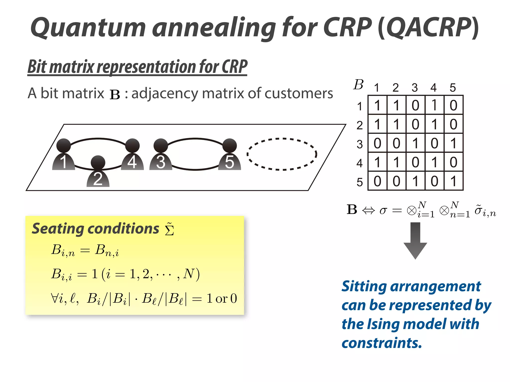
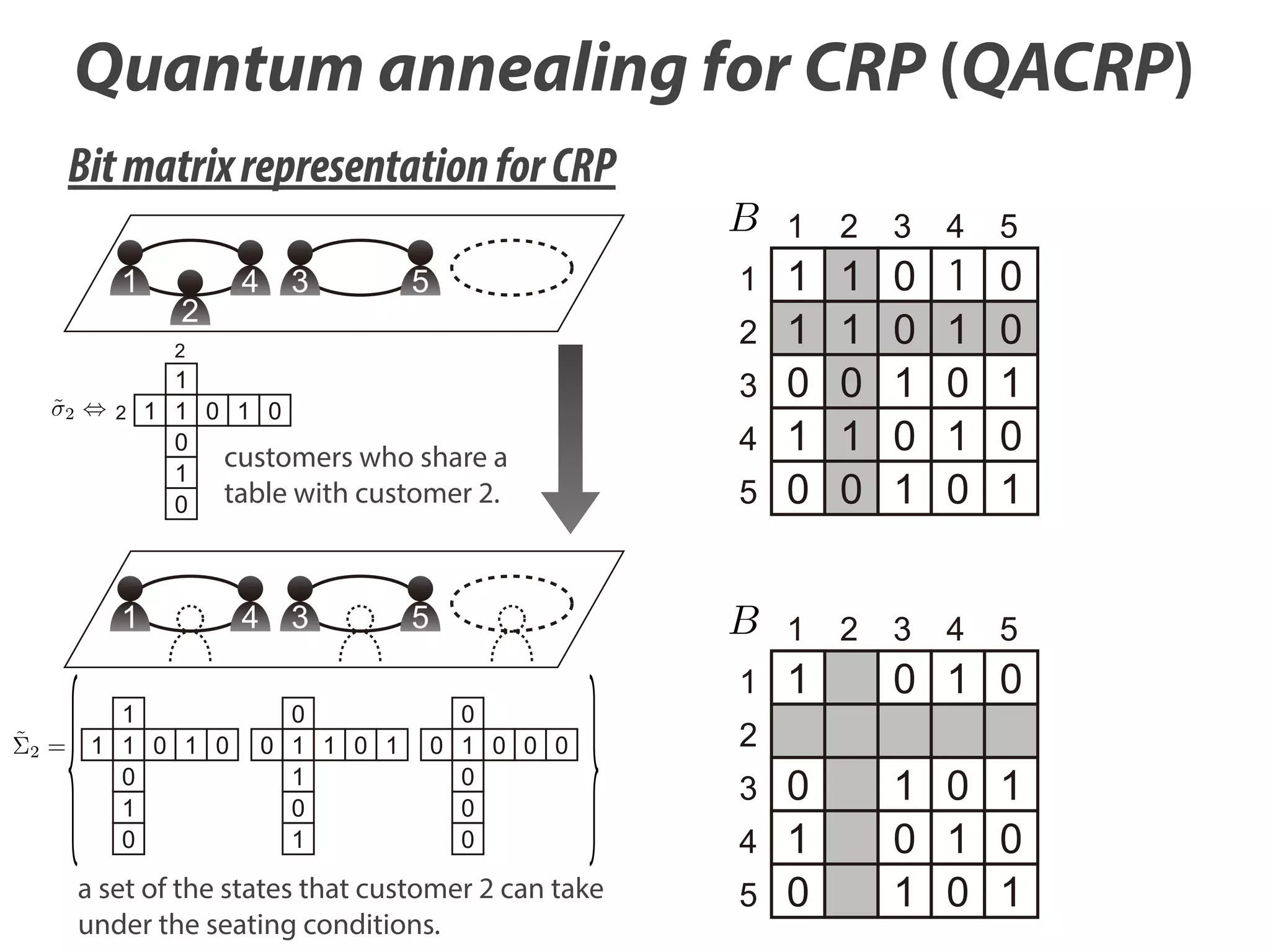
Density matrix representation for “classical” CRP
Hc = diag[E(
E(
( )
)=
p( ) =
(1)
), E(
ln p(
( )
(2)
)
+
T
e
), · · · E(
( )
T e Hc
=:
T
)
)]
˜
( )
Hc
(2
N2
˜
e Hc
Zc
Sitting arrangement can be represented by the
Ising model with constraints.](https://image.slidesharecdn.com/neurocomputing-121-523-slideshare-140107121432-phpapp01/75/Quantum-Annealing-for-Dirichlet-Process-Mixture-Models-with-Applications-to-Network-Clustering-14-2048.jpg)
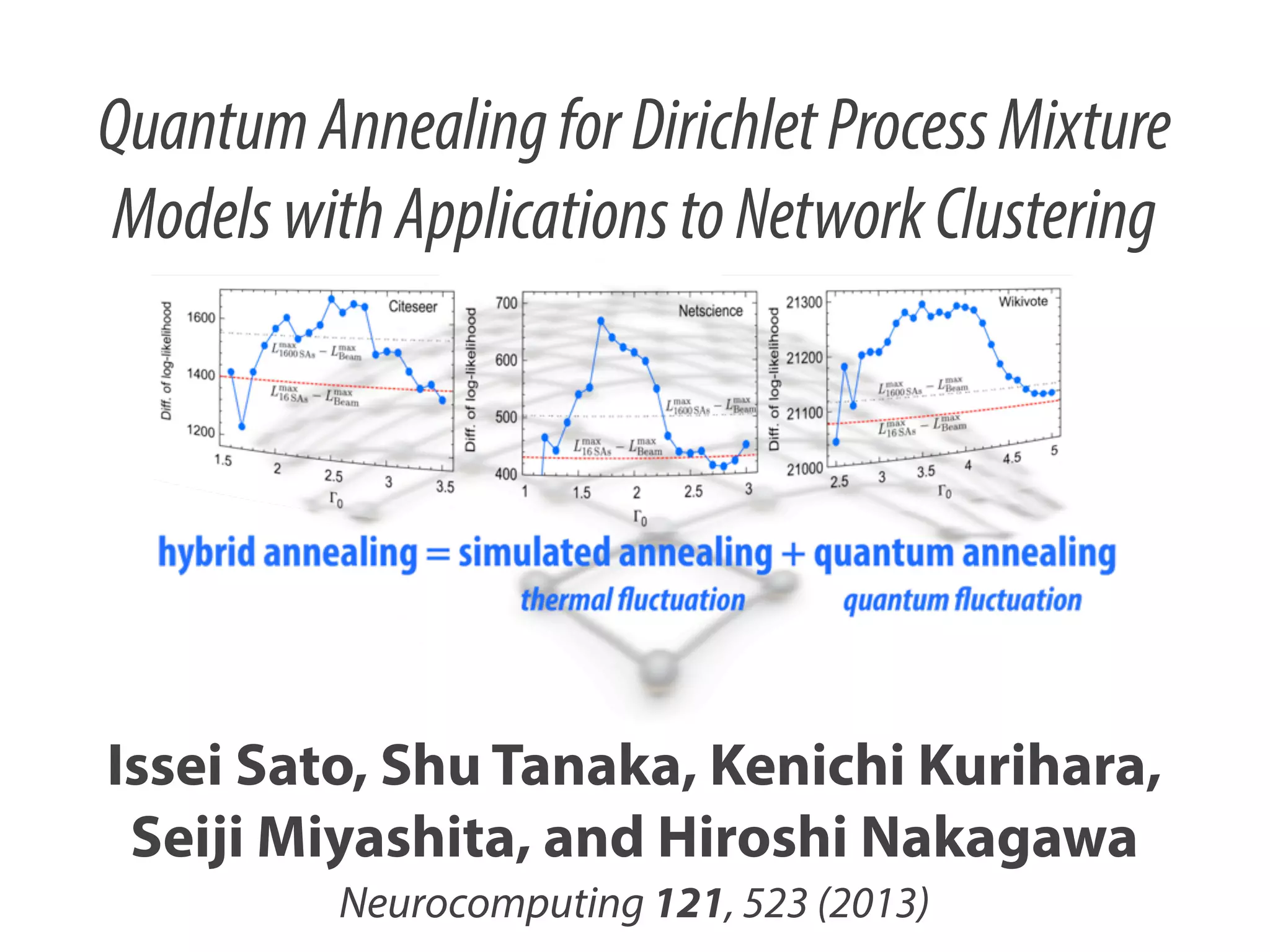
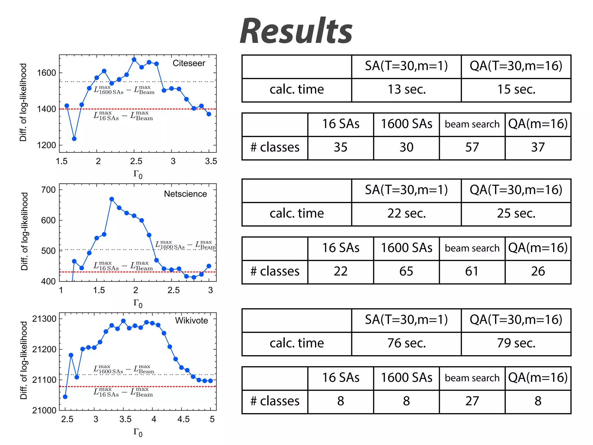
![Diff. of log-likelihood
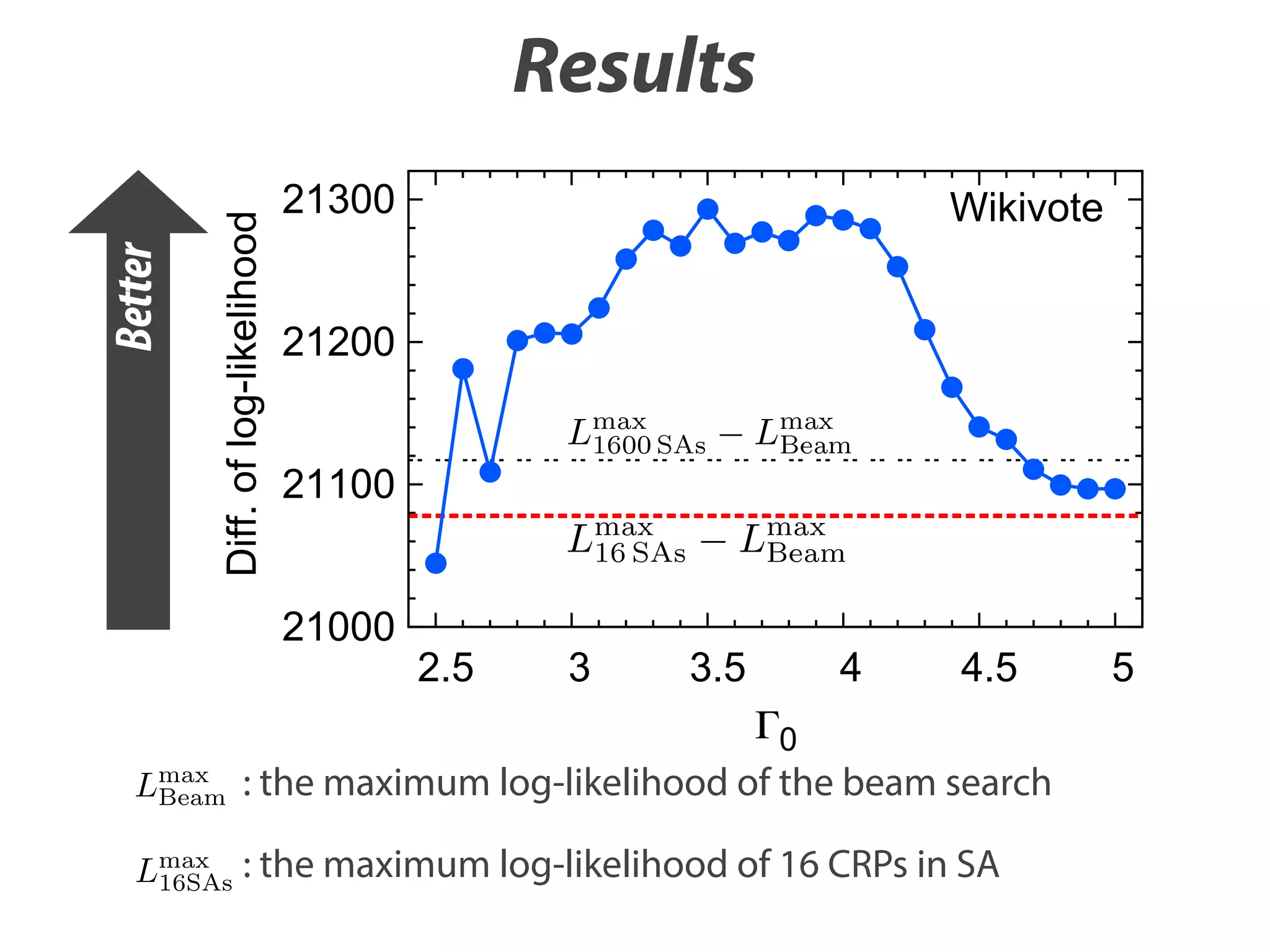
Results
Citeseer
1600
1400
1200
Diff. of log-likelihood
1.5
2.5
3
Netscience
We consider multiple running CRPs in which sj ðj ¼ 1; …; mÞ
indicates the seating arrangement of the j-th CRP and represents
~
the j-th bit matrix Bj . We correspond Bj;i;n ¼ 1 to s j;i;n ¼ ð1; 0Þ⊤ and
⊤
Bj;i;n ¼ 0 to s j;i;n ¼ ð0; 1Þ , which means that we can represent Bj as
~
sj by using Eq. (5). We derive the following theorem:
600
500
1
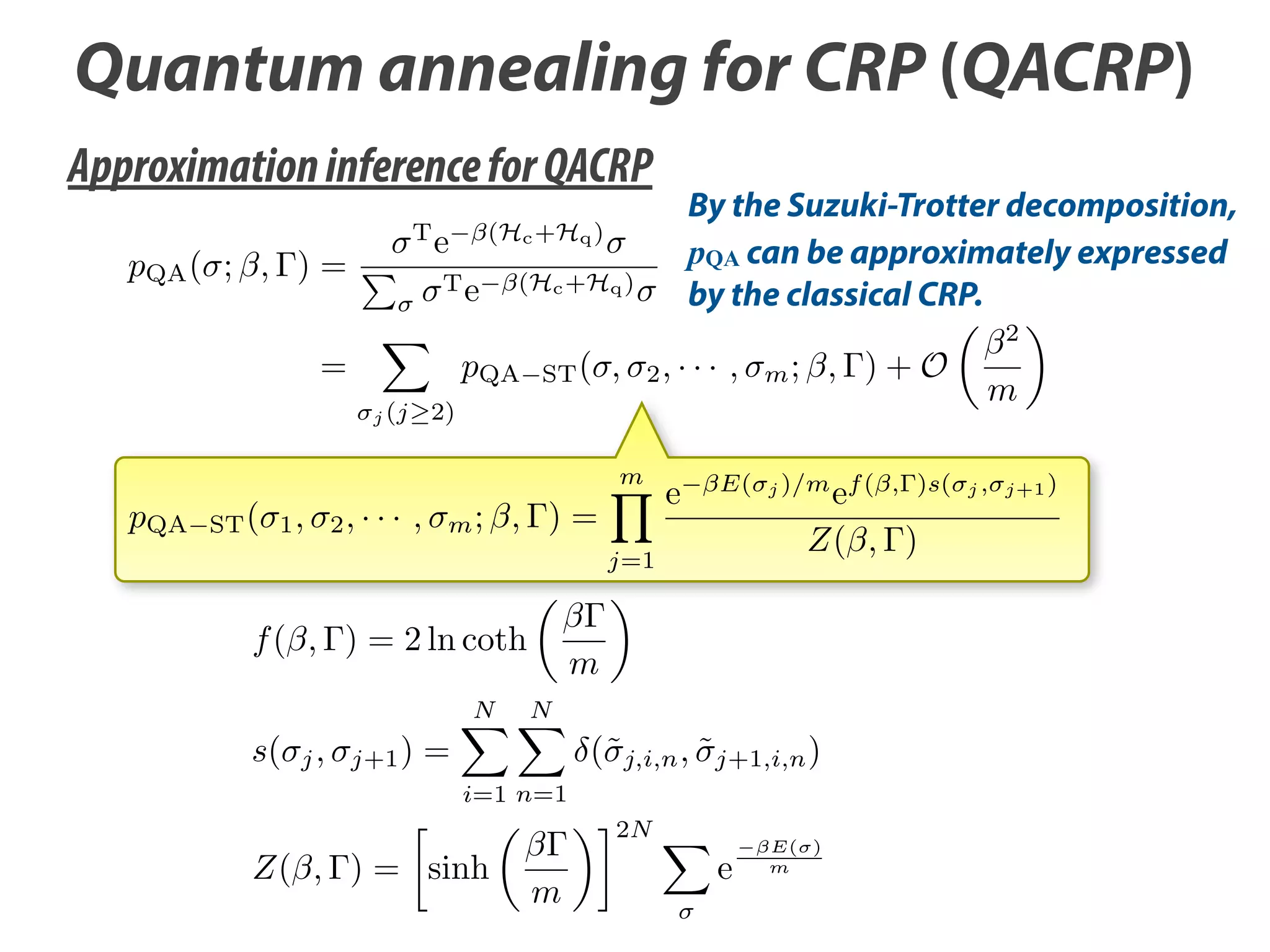
Theorem 3.1. Sato ðs;al. ΓÞ in Eq. (10) is approximated by the Suzuki–
I. pQA et β; / Neurocomputing 121 (2013) 523–531
Trotter expansion as2.5
follows: 3
1.5
2
0
pQA ðs; β; ΓÞ ¼
21300
1 ⊤ −βðHc þHq Þ
s e
s
Z
Wikivote
¼ ∑ pQA−ST ðs; s2 ; …; sm ; β; ΓÞ þ O
sj ðj≥2Þ
21200
2
!
β
;
m
pQA−ST ðs1 ; s2 ; …; sm ; β; ΓÞ
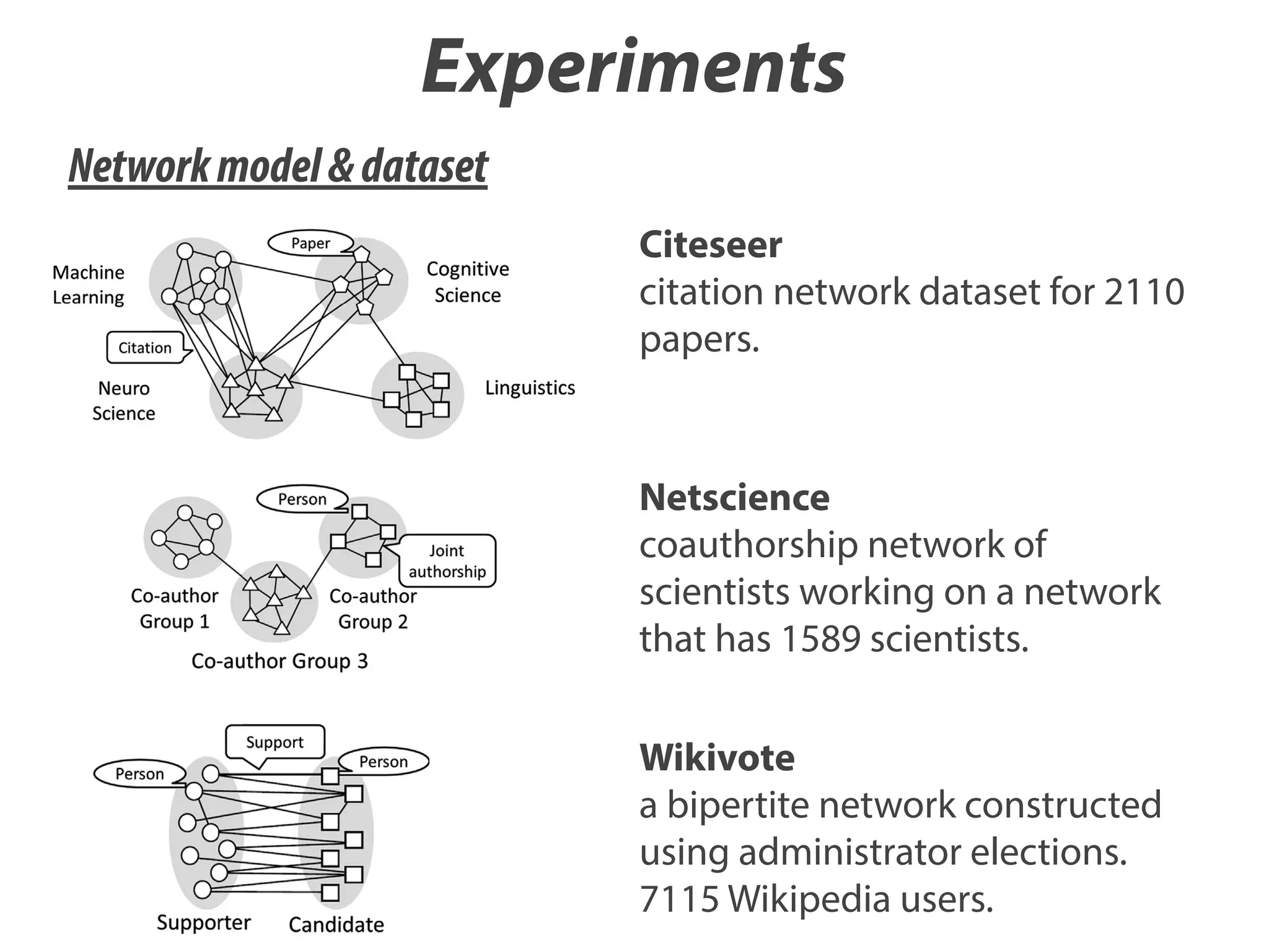
4. Experiments
ð16Þ
We evaluated QA in a real application. We applied QA to a DP
model for clustering vertices in a network where a seati
arrangement of the CRP indicates a network partition.
2.5
1
e−β=mEðsj Þ ef ðβ;ΓÞsðsj ;sjþ1 Þ ;
Zðβ; ΓÞ
j¼1
m
¼ ∏
regarded as a similarity function between the j-th and (j+1)-th
matrices. If they are the same matrices, then sðsj ; sjþ1 Þ ¼ N 2 .
Eq. (2), log pSA ðsj Þ corresponds to log e−β=mEðsj Þ =Z and the regulari
term f Á Rðs1 ; …; sm Þ is log ∏m 1 ef ðβ;ΓÞsðsj ;sjþ1 Þ ¼ f ðβ; ΓÞ∑m 1 sðsj ; sjþ
j¼
j¼
Note that we aim at deriving the approximation inference
pQA ðs i jss i ; β; ΓÞ in Eq. (13). Using Theorem 3.1, we can der
~
~
527
Eq. (4) as the approximation inference. The details of the deriv
tion are provided in Appendix B.
ð15Þ
where we rewrite s as s1 , and
21100
21000
I. Sato et al. / Neurocomputing 121 (2013) 523–531
3.5
Fig. 5. Examples of network structures. (a) Social network (assortive network), (b) election network (disassortative network) and (c) citation network (mixture of assorta
and disassortative network).
0
700
400
Diff. of log-likelihood
2
Better solution
can be obtained
by QA.
β
Γ ;
ð17Þ
f ðβ; ΓÞ ¼ 2 Fig. 5. Examples of network structures. (a) Social network (assortive network), (b) election network (disassortative network) and (c) citation netwo
log coth
m
4.1. Network model
and disassortative network).
3
3.5
4
N
4.5
5
N
~
~
sðsj ; sjþ1 Þ ¼ 0∑ ∑ δðs j;i;n ; s jþ1;i;n Þ;
ð18Þ
We used the Newman model [17] for network modeling in t](https://image.slidesharecdn.com/neurocomputing-121-523-slideshare-140107121432-phpapp01/75/Quantum-Annealing-for-Dirichlet-Process-Mixture-Models-with-Applications-to-Network-Clustering-21-2048.jpg)
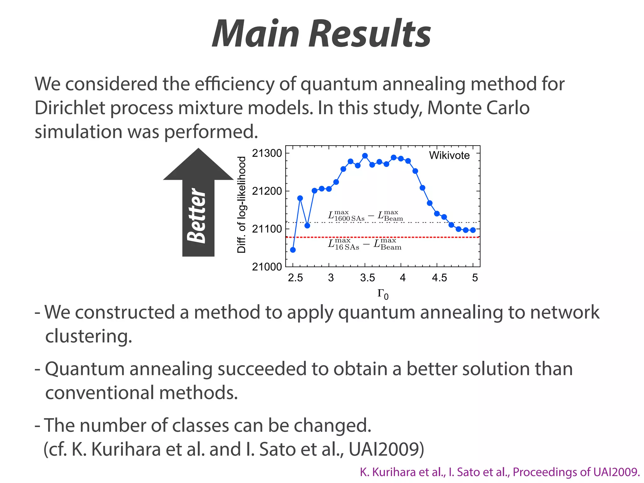

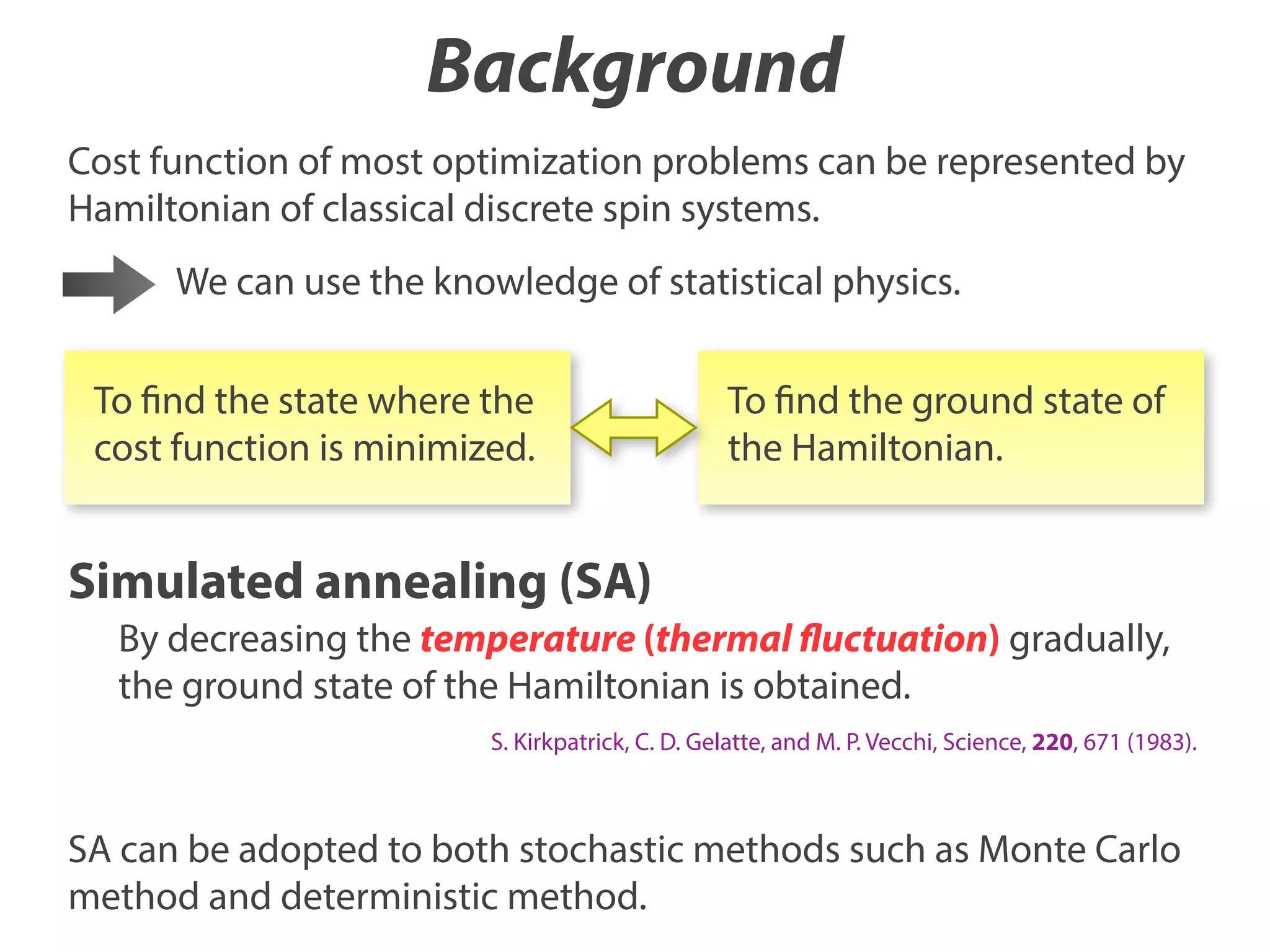
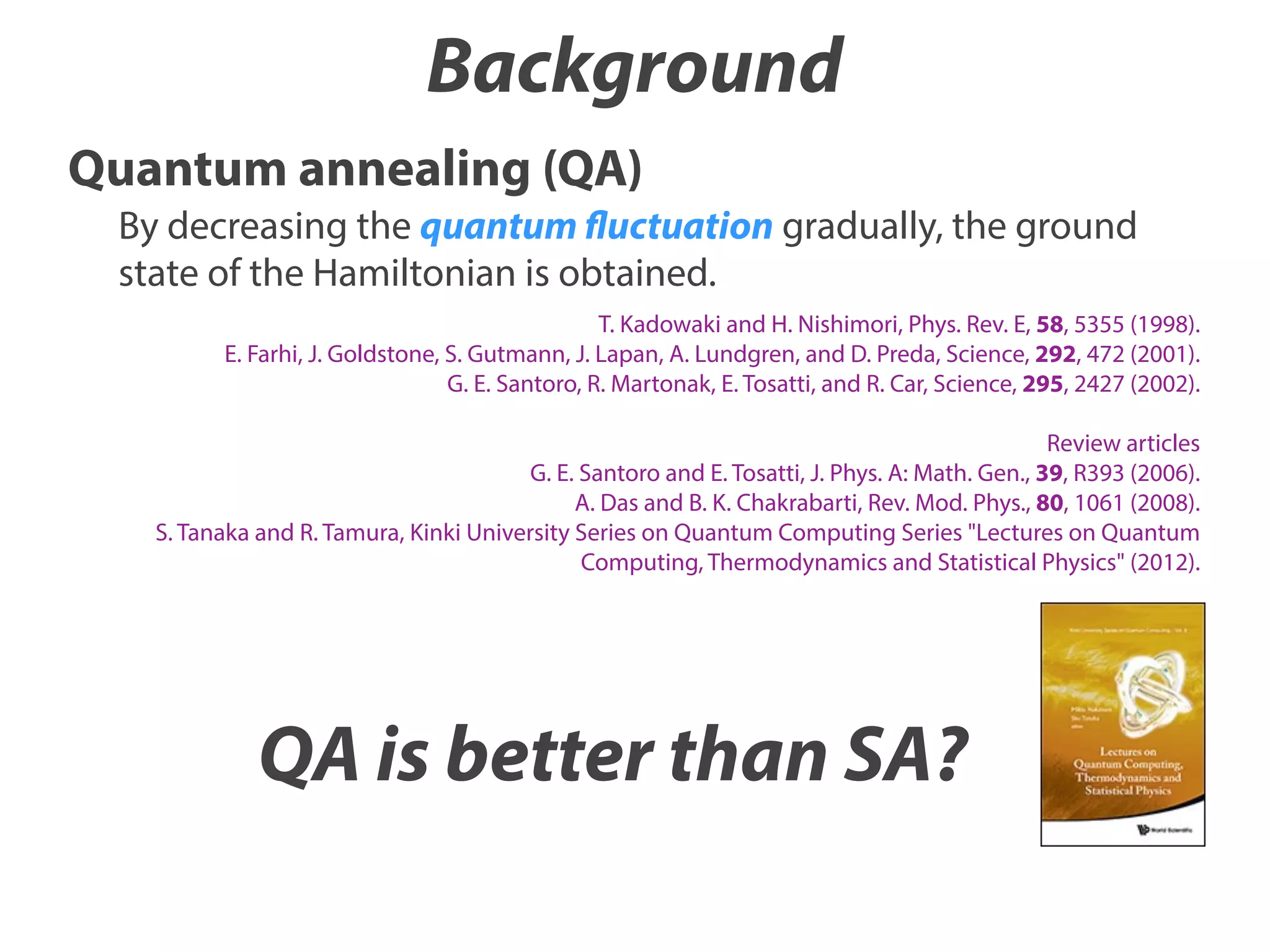
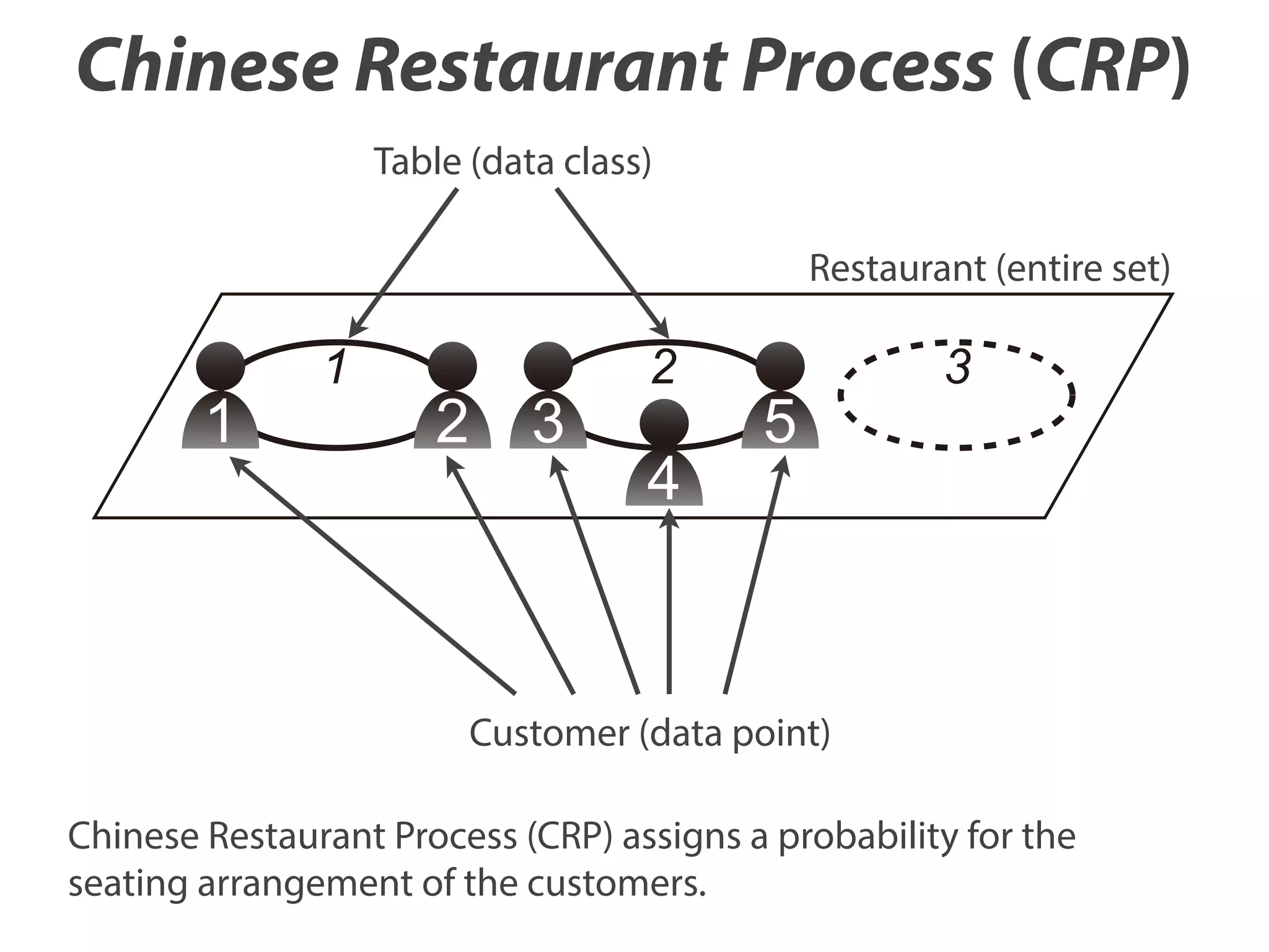
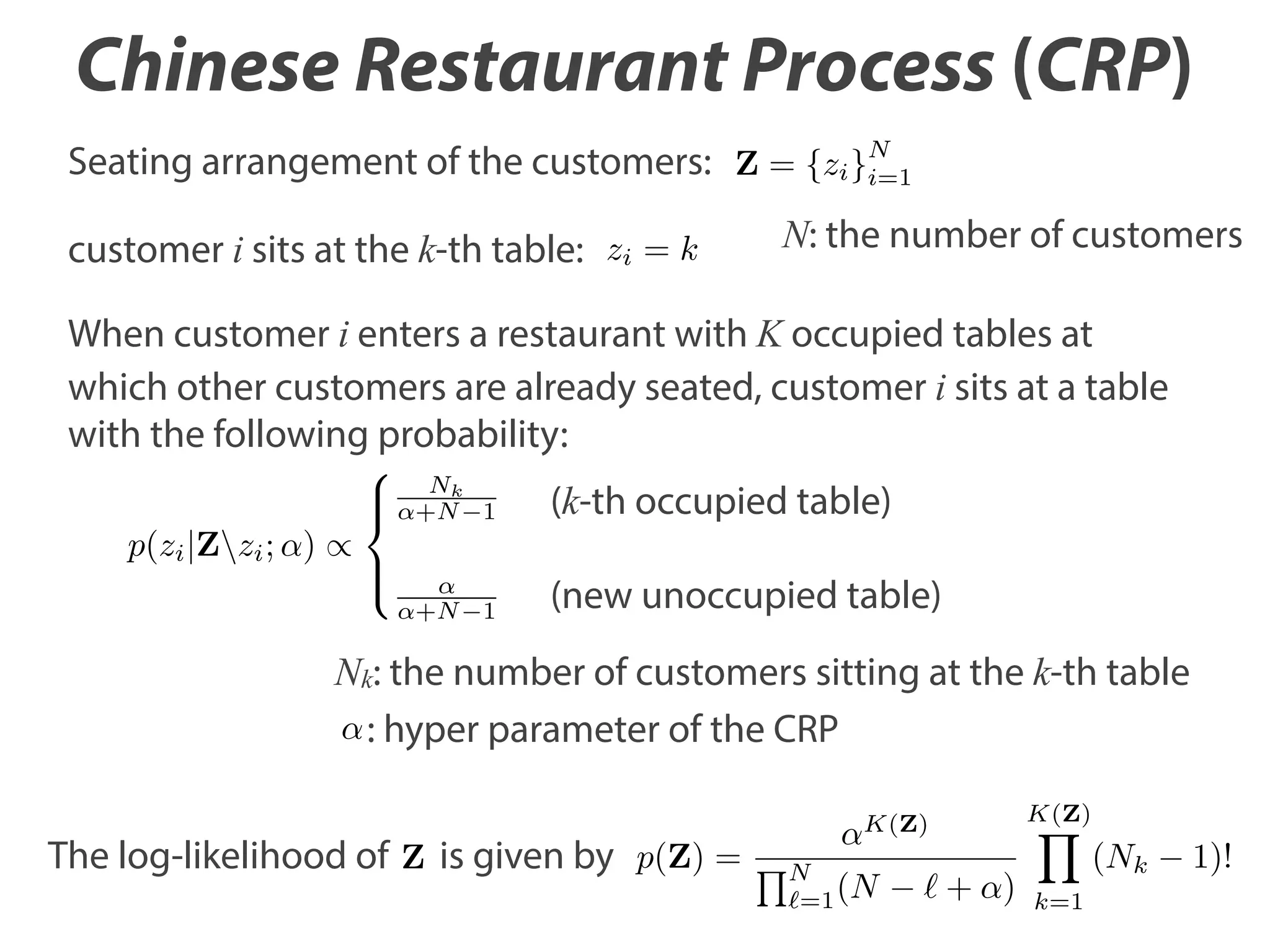
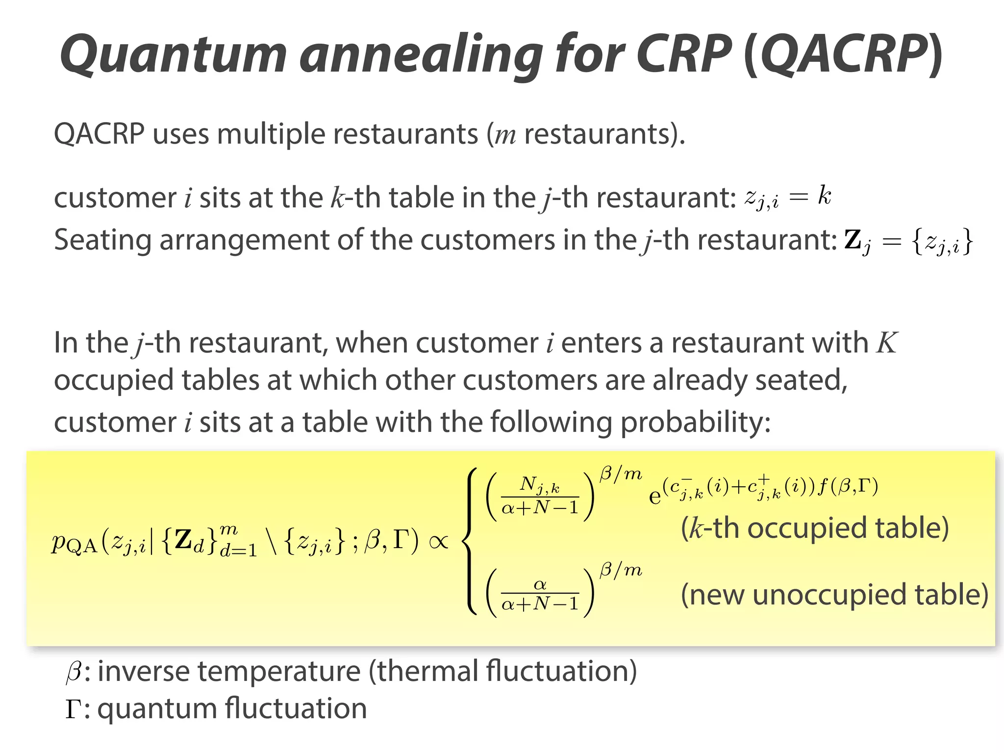
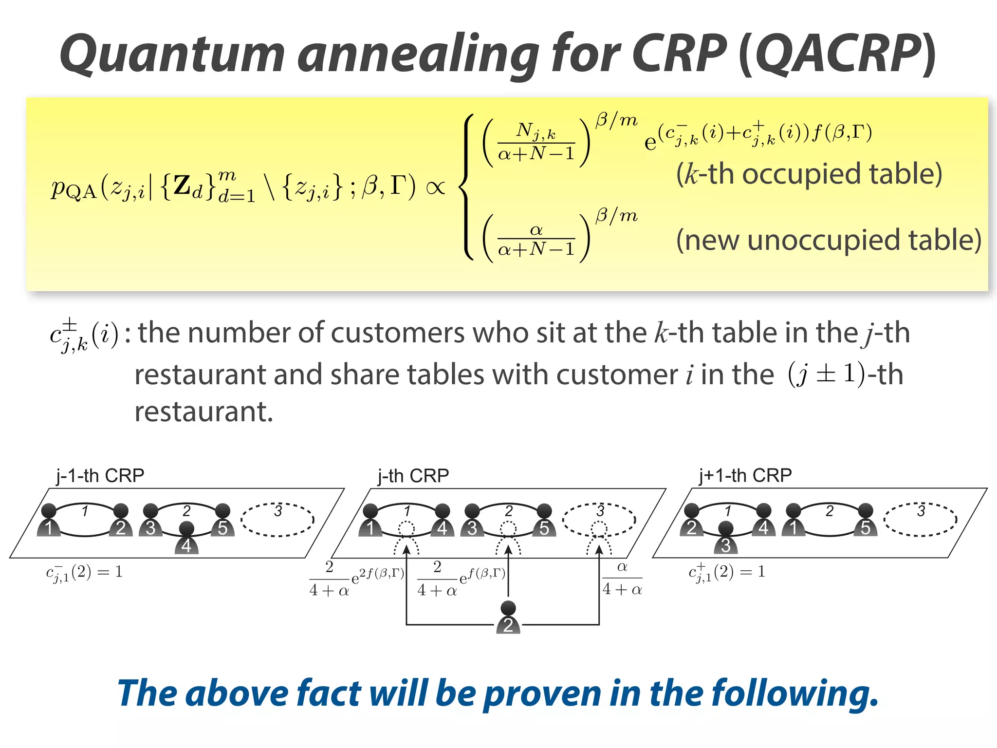
The document discusses the application of quantum annealing to Dirichlet process mixture models for network clustering, showing that this method yields better solutions than conventional techniques. It details the background optimization problems and introduces a new framework called QACRP (Quantum Annealing for Chinese Restaurant Process), which utilizes multiple 'restaurants' for improved seating arrangements of data points. The study validates the effectiveness of quantum annealing through Monte Carlo simulations applied to various network datasets.