1. Qubit: The Unit of Quantum Computation
1 Introduction
The basic constituent of a quantum computer is a quantum bit or "qubit", which owes its
name to the more familiar classical "bit". The bit, itself an abbreviation of "binary digit",
can take two values 0 and 1, which in a modern-day computer correspond to a transistor
being in on or off states respectively. The quantum bit is a state vector, having two basis
states that are labelled |0 and |1 . From our knowledge of quantum mechanics we know
that a qubit can exist in a superposition of |0 and |1 , quite unlike a classical bit. This and
other quantum mechanical properties give quantum computers several unique features
that can be exploited to design novel algorithms and computational techniques.
2 The qubit: representation
2.1 The |0 , |1 basis
The mathematical representation of a qubit is a point in two dimensional Hilbert space.
A set of basis vectors in a 2D Hilbert space are given by,
|0 =
1
0
; |1 =
0
1
(1)
The most general qubit is represented as,
|ψ = α|0 + β|1 , (2)
where, α and β are in general complex numbers and are the probability amplitudes of the
system to be in the two respective states. The basis state {|0 , |1 } is known as the standard
basis or the computational basis in 2D Hilbert space for the purpose of measurements.
When we measure this qubit given in (2) in the standard basis, the probability of outcome
corresponding to |0 is |α|2
and the probability of outcome corresponding to |1 is |β|2
.
2.2 The Bloch sphere
Since the net probability is one, |α|2
+ |β|2
= 1 the qubit given in (2) can be represented in
spherical polar coordinates as,
|ψ = e
−iφ
2 cos
θ
2
|0 + e
iφ
2 cos
θ
2
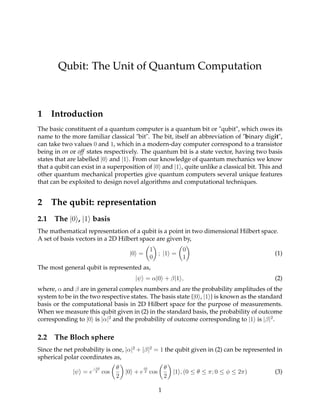
|1 , (0 ≤ θ ≤ π; 0 ≤ φ ≤ 2π) (3)
1
2. A qubit is thus a point on the surface of a sphere of unit radius, parametrized by the
coordinates (θ, φ) as represented in Fig. 1. The basis states |0 and |1 are then represented
by the north and south poles of the Bloch sphere respectively. The convenience of the
Bloch sphere representation of a qubit will be evident when we study the evolution of
qubits and quantum gates.
Figure 1: Representation of a qubit in Bloch sphere.
Physical realisation of a qubit can be in many forms. Any two level quantum mechanical
system can be a qubit, Prominent examples being the up (| ↑ = |0 ) and down (| ↓ = |0 )
spin states of an electron, or vertical and horizontal polarization states of a photon, or the
ground and excited states of an atom.
3 Operators in H2
3.1 Pauli matrices
The three Pauli matrices σx, σy, σz are both hermitian and unitary matrices that prove
very useful for studying two-level quantum systems. They satisfy σ2
x = σ2
y = σ2
z = 1. It is
straight forward to check that σx, σy, and σz have two eigenvalues 1
2
and −1
2
, physically
corresponding to two measurable spin angular momentum values of the electron along
x, y and z directions respectively.
For convenience, we have chosen the spin along z-direction to be the diagonal matrix σz.
The eigenvectors of this matrix we are already familiar with, |0 (corresponding to up-
spin) and |1 (corresponding to down-spin), with eigenvalues ±1 respectively.
The eigenvectors of σx, on the other hand, are,
|± =
1
√
2
(|0 ± |1 ) (4)
2
3. Measuring spin: For appreciating the intricacies of quantum mechanics and its connec-
tion with the classical world, let us consider an eigenstate of σx, |+ = 1√
2
(|0 + |1 ). This
corresponds to a spin-1
2
particle with its spin oriented along the +x direction. On the
other hand, this is also an equal superposition of the spin-up and spin-down states along
z-direction. Classical reasoning suggests that a measurement of spin along z-direction for
the above state should yield zero, since z and x directions are orthogonal to each other.
But, as is evident, a measurement of spin along z actually yields ±1
2
with equal probabil-
ities. In other words, the |+ collapses to either |0 or |1 with probability 1
2
.
The expected classical picture emerges if we perform a large number of measurement,
where the average measurement of spin smooths out to 0. A single measurement, how-
ever, always give either +1
2
or −1
2
.
3.1.1 Properties of Pauli matrices
The Pauli matrices are essential in studying quantum information theory and quantum
computation. It is therefore worth examining their properties in some detail. It is easy to
check that they obey the commutation relations,
σiσj − σjσi = [σi, σj] = 2 ijkiσk (5)
where {i, j, k} ∈ {x, y, z}.
This is structurally similar to the relation satisfied by the components of the orbital angu-
lar momentum L = r × p.
Further,
σiσj + σjσi = 2δij (6)
We can condense (5) and (6) into the useful relation:
σiσj = δijI + i ijkσk (7)
It should also be added that the Pauli matrices with the 2 × 2 identity matrices form
a complete basis in the space of 2 × 2 matrices. Any operator in H2 can therefore be
expanded as
A = a0I + a.σ (8)
3.2 Maximally unbiased basis
Let us start with the matrix σy =
0 −i
i 0
.
We wish to diagonalize it. The eigenvalues equation reads, σyψ = λψ, where ψ =
ψ1
ψ2
.
with ψ2
1 + ψ2
2 = 1. From the characteristic equation, Detσy − Iλ = 0 one gets
Det
−λ −i
i −λ
=⇒ λ2
− 1 = 0 =⇒ λ = ±1 (9)
3
4. For λ = 1, ψ can be found from the equation
−1 −i
i −1
ψ1
ψ2
= 0 =⇒
−ψ1 − iψ2 = 0
iψ1 − ψ2 = 0
=⇒ ψ2 = iψ1
The normalization condition yields,
ψ1 ψ2
ψ1
ψ2
= 1 =⇒ 2|ψ2
1| = 1
This gives ψ1 = 1√
2
eiθ
, with θ as an arbitrary phase.
An overall phase of a wave function is not a measurable quantity inquantum mechanics
which allows us to write,
ψ+1 = 1√
2
1
i
, ψ−1 = 1√
2
1
−i
From the eigenvectors, a unitary matrix can be constructed,
U+1 = 1√
2
1 1
i −i
, such that, U−1
+1 σyU+1 =
1 0
0 −1
.
This physically amounts to rotating the spin operator σy along the y-direction to the z-
direction with
σz =
1 0
0 −1
Analogously one finds that for Sy the eigenvectors are 1√
2
1
1
, 1√
2
1
−1
and as noted
earlier for σz, these two are
1
0
,
0
1
. To summarize we have obtained three sets of
orthogonal vectors,
1
0
,
0
1
1
√
2
1
1
,
1
√
2
1
−1
1
√
2
1
i
,
1
√
2
1
−i
In the space of two dimensional column vectors there are two independent vectors and
hence any two of the above set will supplies to describe a general vector, e.g., |ψ =
α |0 + β |1 . It is worth emphasizing that a member of a given set is not orthogonal to
another member of a different set. In fact, it can be easily checked that the magnitude of
their overlap is equal to 1√
2
. For example,
1
√
2
1 1
1
√
2
1
i
=
1
√
2
|1 + i| =
1
√
2
4
5. This fact plays a crucial role in the theory of quantum measurement and quantum com-
munication theory. These type of basis sets are known as maximally unbiased basis
(MUB). In N dimension, we need to construct N + 1 sets , each set containing N orthog-
onal vectors. The magnitude of the overlap from one set with any other from a different
set is 1√
N
.
3.3 Rotation operators
The 2D operators,
Rˆn(θ) = e
iθ
2
σ·ˆn
(10)
where ˆn is a unit vector, are known as rotation operators as their action on qubits is to
rotate them through an angle θ along an axis ˆn on the Bloch Sphere.
On expanding the exponential and using the identity (σ · ˆn)2
= I, we get the following
relation
Rˆn(θ) = I cos
θ
2
+ ˆn.σ sin
θ
2
(11)
These rotation operators prove useful for constructing different quantum gates.
4 Quantum gates
In classical computation, complex tasks are performed using algorithms that implement
a sequence of simpler logic operations on bits. These operations are commonly referred
to as gates, e.g., the NOT-gate that performs a bit-flip, i.e. changes 0 to 1 and 1 to 0, the
OR- and AND-gates, etc. The quantum analogue of these logic gates are the 2D unitary
operators that we have studied in the previous section.
4.1 Single-qubit gates
Let us now look at some important single-qubit gates.
4.1.1 Quantum NOT-gate
First, we construct a quantum version of a NOT-gate. The gate should change |0 to |1
and |1 to |0 . It is easy to see that the Pauli matrix σx fulfils the criteria:
0 1
1 0
1
0
=
0
1
,
0 1
1 0
0
1
=
1
0
Thus, σx acts as the NOT gate on the computational basis states. However, note that
it need not act similarly on other basis; in particular, the eigenstates of σX remain un-
changed under this operation.
A quantum computer can go much beyond replicating the familiar logic operations of
classical computers, as evident from our the following example - the uniquely quantum
5
6. √
NOT-gate.
To construct this gate, we note that the NOT-gate can be expressed, up to a phase, as a
rotation of π about the x-axis,
σx =
0 1
1 0
= iRx(π) (12)
Since an overall phase is not important in quantum mechanical calculations, the
√
NOT-
gate is given (again up to an overall phase) by a rotation of π/2 about the x-axis,
√
NOT = Rx(π/2) =
1
√
2
1 −i
−i 1
(13)
4.1.2 Hadamard gate
The matrix H = 1√
2
1 1
1 −1
diagonalizes σx:
H†
σxH =
1 0
0 −1
(14)
which takes the state |0 to a linear superposition:
H |0 =
|0 + |1
√
2
(15)
The above operator is called the Hadamard gate, another important single qubit gate. The
Hadamard gate takes the computational basis states to the σx basis, |± .
Another operator ˜H = 1√
2
1 1
−1 1
is a unitary but non-Hermitian matrix such that
˜H† 0 1
1 0
˜H =
−1 0
0 1
Note that
˜H |0 =
1
√
2
1 1
−1 1
1
0
=
1
√
2
1
−1
=
1
√
2
|0 −
1
√
2
|1
However, ˜H12
= I, unlike H4
= I. The physical meaning of the above operations should
be explored by the enthusiastic reader.
4.1.3 Phase gate
The phase gate,
S =
1 0
0 i
(16)
6
7. introduces a relative phase of π in a superposition of computational basis states:
S
|0 + |1
√
2
=
|0 + i|1
√
2
(17)
The
√
NOT, the Hadamard and the phase gate are all examples of quantum gates that do
not have analogues in classical computation. Any 2 × 2 unitary operator can be used as
an elementary logic operation as per our need.
4.2 Decomposition of single-qubit gates
While obtaining the matrix form of the
√
NOT gate, we expressed the NOT gate as a
rotation operator. More generally, any single qubit unitary operation can be written as
U = eiα
Rˆn(θ), i.e., a rotation followed by a global phase shift.
Any single qubit gate can be decomposed into various combinations of rotations and
global phase shifts. A particularly important decomposition is the Z-Y decomposition:
U = eiα
Rz(β)Ry(γ)Rz(δ)
Such decompositions can in fact be carried out in terms of rotations along any two non-
parallel axis ˆn and ˆm: U = eiα
Rˆn(β)Rˆm(γ)Rˆn(δ).
Using the Z-Y decomposition, we can arrive at another useful representation of 2 × 2
unitary operators:
U = eiα
AσxBσxC (18)
where A, B, C are unitary and ABC = I.
5 Composite systems
Composite or multi-partite systems can be represented in quantum mechanics using the
notion of tensoor-product space. Suppose you have two systems A and B in states |ψ1 A
and |ψ2 b respectively. The state of the composite system A+B can be written in the form
|ψ1 A ⊗|ψ2 B where ⊗ denotes the tensor product. For example, using qubit states |0 and
|1 one can describe the two particle computational basis in the form
1
0
⊗
1
0
= |0 ⊗ |0 = |00 =
1
0
0
0
|01 =
0
1
0
0
, |10 =
0
0
1
0
, |11 =
0
0
0
1
These are four orthogonal vectors describing four particles. They are independent too,
therefore forming a basis in the composite four-dimensional Hilbert Space. The product
7
8. state, along with superposition of probability amplitudes in quantum mechanics give rise
to a bizarre quantum mechanical phenomenon called entanglement. Consider the state
1
√
2
1
0
0
0
+
1
√
2
0
0
0
1
1
√
2
1
0
0
1
produced by the superposition of two product states:
1
√
2
1
0
0
1
=
1
2
|0 0 +
1
√
2
|1 1
This state can be written as a product of single-qubit states,
1
√
2
1
0
0
1
= |ψ1 ⊗ |ψ2
unlike say,
1
0
0
0
= |0 ⊗ |0
=
1
0
⊗
1
0
The former is a non-separable or entangled state, which plays a very important, almost
magical role in quantum computation.
6 Multi-qubit gates
Previously we have only looked at local operations, i.e., gates that act at the level of single
qubits. Quantum gates that act on multiple qubits are necessary for implementing several
quantum algorithms and can be easily constructed (at least theoretically).
6.1 CNOT gate
The classic example of such a gate is the two-qubit controlled-NOT or CNOT-gate. It takes
as input a control and a target qubit and executes a NOT operation on the target only if the
control is in the state |1 . If the control is set to |0 , nothing happens to the target.
8
9. 6.1.1 Action of CNOT on H4 computational basis
|00
CNOT
−−−−→ |00 , |01
CNOT
−−−−→ |01
|10
CNOT
−−−−→ |11 , |11
CNOT
−−−−→ |10
6.1.2 Matrix representation
The matrix representation of CNOT is given by:
|0 0| ⊗ I2 + |1 1| ⊗ σx =
1 0 0 0
0 1 0 0
0 0 0 1
0 0 1 0
The CNOT gate belongs to a broad-class of controlled gates that execute some operation
only a control-qubit is set to the |1 state. An (n+1)-dimensional controlled-U-gate, where
U is an n-dimensional operator can be expressed as:
CU = |0 0| ⊗ In + |1 1| ⊗ U (19)
6.2 Universality of gates
Any arbitrary unitary operation, in any dimensions, can be decomposed into sequences
of single-qubit operations and the CNOT gate. These form, what is called, a universal set
of quantum gates. Any operation conceivable in a quantum computer can be expressed
in terms of such an universal set. In particular, as any single qubit operation can be
expressed as a finite sequence of rotations, the rotation operators along with CNOT are
sufficient to construct all other unitary operations.
Note that the universal set so obtained has and infinite number elements. What we would
like is to have a finite universal set but such a set is not sufficient to exactly reproduce
any arbitrary unitary operation. However, we can think of finite sets of gates that can
approximate any unitary operator up to a desirable level of accuracy. One such set is
formed by the Hadamard, the π
8
or R(π
4
) gate and the CNOT gate.
A few examples
Representing multi-qubit states and operators in matrix form can quite often prove con-
fusing. The standard way of expressing two-qubit operators are illustrated with a few
examples so that the reader gets familiarized.
1 ⊗ 1 =
1 0 0 0
0 1 0 0
0 0 1 0
0 0 0 1
9
12. σy ⊗ σz =
0 0 1 0
0 0 0 −1
−1 0 0 0
0 1 0 0
σz ⊗ σy =
0 1 0 0
−1 0 0 0
0 0 0 −1
0 0 1 0
σx ⊗ σz =
0 0 1 0
0 0 0 −1
1 0 0 0
0 −1 0 0
σz ⊗ σx =
0 1 0 0
1 0 0 0
0 0 0 −1
0 0 −1 0
Problems
1. A = σx⊗σx and B = σy ⊗σy. Find the eigenstates. Do these two operators commute?
2. Show that eiθσ/2
= cos(θ/2)I + isin(θ/2)(σ · ˆn).
3. Calculate Tr[ei¯σ.¯a
ei¯σ.¯b
].
4. Show that controlled NOT gate is Hermitian and Unitary.
5. Write down the matrix representation for the controlled-Z gate.
6. Compute the expectation values of the operators σi ⊗ σj on the state vector
|ψ >= c|00 > +α|01 > +β|10 > +γ|11 > ,where the overall phase factor (up to
which |ψ > is defined) is chosen so that c is real (while α, β and γ are complex
numbers).
7. Consider the singlet state,
|ψ = 1√
2
[| ↑ 1| ↓ 2 − | ↓ 1| ↑ 2], where | ↑ =|0 =
1
0
and | ↓ =|1 =
0
1
are two
orthogonal states.
(a) Show that the quantum mechanical expectation value,
E(n, m) = ψ|σ.n ⊗ σ.m|ψ , is given by E(n, m) = −cosφn,m,
where, φn,m is the angle between unit vectors ˆm and ˆn. [2]
(b) The CHSH-inequality is given by,
|E(n, m) − E(n, m )| + |E(n , m ) + E(n , m)| ≤ 2.
Find the angles where the inequality is maximally violated. Interpret the result.
12
13. 8. Given the Pauli spin matrices σx, σy and σz, find out the eigenvalues and the eigen-
vectors of the matrix e
−→σ .ˆn
, where ˆn is the unit vector on the Bloch sphere, given by
ˆn = (sin θ cos φ, sin θ sin φ, cos θ) and −→σ = ˆi σx + ˆj σy + ˆk σz.
(a) Express the eigenvectors in terms of the computational basis {|0 , |1 }
(b) Show explicitly using the different rotation matrices expressed in terms of the
Euler angles, how you will arrive at these eigenstates from the state |0 in the
Bloch sphere.
9. Prove that (a.σ)(b.σ) = (a.b)I + iσ.(a × b).
10. Compute the expectation values of the operators σi ⊗ σj on the state vector |ψ =
c|00 + α|01 + β|10 + γ|11 ,where the overall phase factor (up to which |ψ is
defined) is chosen so that c is real (while α, β and γ are complex numbers)
11. (a) Write down the truth table for the Toffoli Gate (a gate for reversible classical
computation, also known as the controlled-controlled-NOT gate) which acts
on three bits as follows: It flips the state of the third bit iff both the first and
the second bits are in the state 1.
(b) Suppose one represents the 8 possible states of the three bits by column vectors
as follows:
000 ≡
1
0
0
0
0
0
0
0
; 001 ≡
0
1
0
0
0
0
0
0
; 010 ≡
0
0
1
0
0
0
0
0
; 011 ≡
0
0
0
1
0
0
0
0
;
100 ≡
0
0
0
0
1
0
0
0
; 101 ≡
0
0
0
0
0
1
0
0
; 110 ≡
0
0
0
0
0
0
1
0
; 111 ≡
0
0
0
0
0
0
0
1
Construct the 8×8 matrix operator G which corresponds to the action of Toffoli
Gate on the above vectors.
(c) Show that G†
G = I, where G†
is the adjoint operator of G (transpose of complex
conjugate of G) and I is 8×8 the identity operator (this proves that G is a unitary
operator, and thereby a valid quantum gate; use a clever method of identifying
known matrices inside the gate before multiplying).
13
14. References
[1] M.A. Nielsen & I.L. Chuang, Quantum Computation and Quantum Information, Cam-
bridge University Press, ISBN 9781107002173
[2] John Preskill, Lecture Notes on Quantum Computation
[3] David Deutsch, Lectures on Quantum Computation
14