QMSS Capability Analysis - Sample Slides
•Download as PPT, PDF•
0 likes•234 views

These are sample slides from our course. Entire presentation can be purchased and downloaded from http://www.qmss.biz/store.asp

Recommended
Recommended
More Related Content
Recently uploaded
Recently uploaded (20)
Featured
Featured (20)
QMSS Capability Analysis - Sample Slides
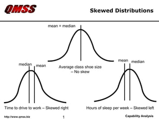
- 1. Skewed Distributions mean = median mean median median mean Average class shoe size – No skew Time to drive to work – Skewed right Hours of sleep per week – Skewed left http://www.qmss.biz 1 Capability Analysis
- 2. Standard Deviation Standard Deviation (σ) = the average difference of each value from the mean √ Σ(x - )2 Std dev = n -1 It is a measure of how spread apart each individual data point is from the mean http://www.qmss.biz 2 Capability Analysis
- 3. What is Cp? Cp is a measure of how well the variation in the data can fit within the tolerance limits If the variation (6σ) is less If the variation (6σ) is greater than the tolerance limits, you than the tolerance limits, you have acceptable variation have unacceptable variation LL UL LL UL 6σ 6σ http://www.qmss.biz 3 Capability Analysis
- 4. Examples USL Cpk = 0.33 15.87% Predicted failure rate -3 -2 -1 0 +1 +2 +3 http://www.qmss.biz 4 Capability Analysis
Editor's Notes
- A good example where the median and mean differ is when you are looking at data that is skewed to the high or low side. Skewed distributions are typical in housing prices, salaries and most time measurements. The middle curve shows a distribution that does not exhibit skewness. Determining the mean and the median will give you almost the exact same result. Now let’s look at the skewed distributions. As you can see, the median typically determines the middle of the data set that is near the top of the curve. The mean calculates the middle further down the curve, towards the longer tail. Remember, when you have outliers or very large or very small values in your data, the mean calculation gets pulled towards those outliers or values. Conclusion, when using data with a skewed distribution, the median is the more appropriate indicator of the middle of the data. For all other cases, the mean is preferred.
- Standard deviation (or sigma) is typically the more accurate estimate of variation. It is calculated by taking the difference of each data point from the average of the data set. Since the standard deviation utilizes every data point, it is a better estimate of the true variability within the data set than the Range. Let’s take a look at an example
- Cp is a measure of how well the variation in the data can fit within the tolerance limits. In simple terms, if the spread of variation in the data is less than the limits, you will have good capability. We use an outline curve to estimate what the histogram would look like without having to plot the actual points. On the left is an example of good capability. The right side diagram shows unacceptable capability, as the 6 standard deviations (sigma) in the data exceeds the limits.
- If we look at a process with Cpk = .33, we can determine the percent of fallout we might expect from this process. As you can see, the USL is lined up exactly with the +1 standard deviation mark. To determine the percent beyond the USL, we add the three sections together, which equals 15.87% (13.6 + 2.14 + .135). To conclude, when the specification limit is lined up with the +1 standard deviation line, you can expect about 15.87% fallout from the process.