Download to read offline


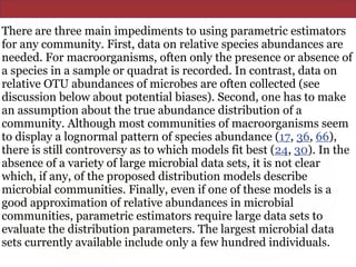


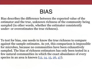
![The Chao1 and abundance-based coverage
estimators (ACE) use this MRR-like ratio to
estimate richness by adding a correction factor to
the observed number of species (9, 11). (For reviews
of these and other nonparametric estimators, see
Colwell and Coddington [14] and Chazdon et al.
[12].)](https://image.slidesharecdn.com/eve161w18-200107155928/85/EVE-161-Winter-2018-Class-9-21-320.jpg)


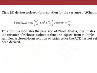
![• http://www.ncbi.nlm.nih.gov/pmc/articles/instance/93182/
equ/M4
which estimates the coefficient of variation of the Fi's (R. Colwell, User's Guide to EstimateS 5 [http://
viceroy.eeb.uconn.edu/estimates]).](https://image.slidesharecdn.com/eve161w18-200107155928/85/EVE-161-Winter-2018-Class-9-26-320.jpg)


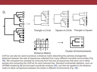

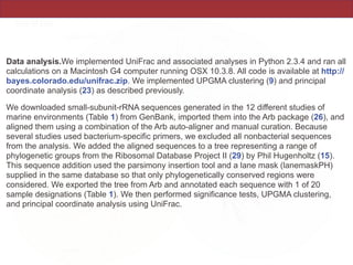


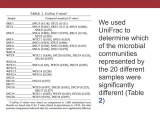


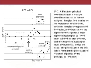
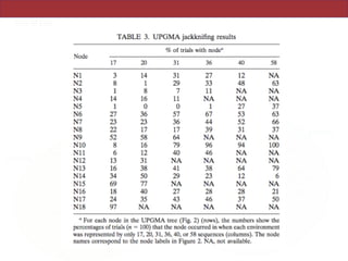


This document summarizes a study on using rRNA sequences to analyze microbial communities from different environments through phylogenetic methods. It introduces the UniFrac metric, which calculates the phylogenetic distance between communities based on the shared and unique branch lengths in a phylogenetic tree of their rRNA sequences. The UniFrac metric can be used to test if communities are significantly different and to generate distance matrices to compare communities through clustering and ordination. The document evaluates UniFrac on data from 12 marine studies and explores how sampling depth affects clustering through jackknifing analyses. UniFrac provides a powerful way to integrate rRNA data from different studies into a single phylogenetic context to address questions about microbial ecology and diversity.