Textbook: An Introduction to Statistical Learning http://faculty.marshall.usc.edu/gareth-james/ISL/

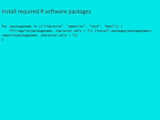
1. Install required R software packages
for (packagename in c("tidyverse", "openxlsx", "ISLR", "boot")) {
if(!require(packagename, character.only = T)) {install.packages(packagename);
require(packagename, character.only = T)}
}

2. Dataset for practice
# Assign the data to an object named "dataset"
# Save the original row numbers as a separate column~!
dataset = ISLR::Auto %>% {add_column(., rownum = 1:nrow(.), .before = 1)} %>% as_data_frame
dataset
# # A tibble: 392 x 10
# rownum mpg cylinders displacement horsepower weight acceleration year origin name
# <int> <dbl> <dbl> <dbl> <dbl> <dbl> <dbl> <dbl> <dbl> <fct>
# 1 1 18 8 307 130 3504 12 70 1 chevrolet chevelle malibu
# 2 2 15 8 350 165 3693 11.5 70 1 buick skylark 320
# 3 3 18 8 318 150 3436 11 70 1 plymouth satellite
# 4 4 16 8 304 150 3433 12 70 1 amc rebel sst
# 5 5 17 8 302 140 3449 10.5 70 1 ford torino
# 6 6 15 8 429 198 4341 10 70 1 ford galaxie 500
# 7 7 14 8 454 220 4354 9 70 1 chevrolet impala
# 8 8 14 8 440 215 4312 8.5 70 1 plymouth fury iii
# 9 9 14 8 455 225 4425 10 70 1 pontiac catalina
# 10 10 15 8 390 190 3850 8.5 70 1 amc ambassador dpl
# # ... with 382 more rows

3. Dataset for practice
dataset %>% str
# Classes ‘tbl_df’, ‘tbl’ and 'data.frame': 392 obs. of 10 variables:
# $ rownum : int 1 2 3 4 5 6 7 8 9 10 ...
# $ mpg : num 18 15 18 16 17 15 14 14 14 15 ...
# $ cylinders : num 8 8 8 8 8 8 8 8 8 8 ...
# $ displacement: num 307 350 318 304 302 429 454 440 455 390 ...
# $ horsepower : num 130 165 150 150 140 198 220 215 225 190 ...
# $ weight : num 3504 3693 3436 3433 3449 ...
# $ acceleration: num 12 11.5 11 12 10.5 10 9 8.5 10 8.5 ...
# $ year : num 70 70 70 70 70 70 70 70 70 70 ...
# $ origin : num 1 1 1 1 1 1 1 1 1 1 ...
# $ name : Factor w/ 304 levels "amc ambassador brougham",..: 49 36 231 14 161 141 54 223 241 2 ...

4. Auto {ISLR} R Documentation
Auto Data Set
Description
Gas mileage, horsepower, and other information for 392 vehicles.
Format
A data frame with 392 observations on the following 9 variables.
mpg
miles per gallon
cylinders
Number of cylinders between 4 and 8
displacement
Engine displacement (cu. inches)
horsepower
Engine horsepower
weight
Vehicle weight (lbs.)
acceleration
Time to accelerate from 0 to 60 mph (sec.)
year
Model year (modulo 100)
origin
Origin of car (1. American, 2. European, 3. Japanese)
name
Vehicle name

6. "Random" sampling to divide training & test data
set.seed(1); rownumber4train = sample(392,196)
rownumber4train %>% dput
# c(105L, 146L, 224L, 354L, 79L, 348L, 365L, 255L, 242L, 24L, 388L,
# 68L, 262L, 391L, 292L, 188L, 270L, 372L, 143L, 290L, 387L, 382L,
# 384L, 47L, 99L, 142L, 5L, 140L, 317L, 124L, 175L, 217L, 178L,
# 67L, 297L, 239L, 283L, 39L, 257L, 379L, 289L, 228L, 275L, 194L,
# 185L, 274L, 9L, 165L, 252L, 238L, 164L, 294L, 149L, 83L, 383L,
# 34L, 107L, 174L, 222L, 136L, 304L, 98L, 152L, 110L, 214L, 85L,
# 157L, 250L, 28L, 356L, 329L, 376L, 111L, 336L, 330L, 323L, 347L,
# 123L, 245L, 301L, 333L, 334L, 363L, 101L, 234L, 63L, 218L, 38L,
# 75L, 44L, 73L, 18L, 193L, 263L, 233L, 237L, 135L, 121L, 357L,
# 360L, 192L, 103L, 371L, 287L, 183L, 62L, 305L, 137L, 299L, 170L,
# 276L, 206L, 100L, 295L, 42L, 4L, 198L, 29L, 315L, 362L, 321L,
# 296L, 131L, 369L, 203L, 122L, 312L, 55L, 61L, 326L, 151L, 21L,
# 10L, 167L, 240L, 154L, 144L, 271L, 251L, 129L, 173L, 380L, 60L,
# 65L, 181L, 112L, 303L, 288L, 26L, 211L, 340L, 385L, 373L, 109L,
# 120L, 43L, 125L, 313L, 249L, 50L, 359L, 207L, 291L, 179L, 201L,
# 94L, 15L, 76L, 163L, 225L, 386L, 186L, 189L, 86L, 339L, 195L,
# 311L, 160L, 130L, 300L, 307L, 41L, 187L, 106L, 314L, 40L, 284L,
# 370L, 213L, 247L, 256L, 258L, 261L, 375L, 57L, 117L)

7. "Random" sampling to divide training & test data
dataset.train = dataset[rownumber4train, ]
dataset.test = dataset[-rownumber4train, ]
dataset.train
# # A tibble: 196 x 10
# rownum mpg cylinders displacement horsepower weight acceleration year origin name
# <int> <dbl> <dbl> <dbl> <dbl> <dbl> <dbl> <dbl> <dbl> <fct>
# 1 105 13 8 360 170 4654 13 73 1 plymouth custom suburb
# 2 146 24 4 90 75 2108 15.5 74 2 fiat 128
# 3 224 17.5 6 250 110 3520 16.4 77 1 chevrolet concours
# 4 354 31.6 4 120 74 2635 18.3 81 3 mazda 626
# 5 79 26 4 96 69 2189 18 72 2 renault 12 (sw)
# 6 348 34.4 4 98 65 2045 16.2 81 1 ford escort 4w
# 7 365 34 4 112 88 2395 18 82 1 chevrolet cavalier 2-door
# 8 255 20.5 6 225 100 3430 17.2 78 1 plymouth volare
# 9 242 21.5 3 80 110 2720 13.5 77 3 mazda rx-4
# 10 24 26 4 121 113 2234 12.5 70 2 bmw 2002
# # ... with 186 more rows
dataset.test
# # A tibble: 196 x 10
# rownum mpg cylinders displacement horsepower weight acceleration year origin name
# <int> <dbl> <dbl> <dbl> <dbl> <dbl> <dbl> <dbl> <dbl> <fct>
# 1 1 18 8 307 130 3504 12 70 1 chevrolet chevelle malibu
# 2 2 15 8 350 165 3693 11.5 70 1 buick skylark 320
# 3 3 18 8 318 150 3436 11 70 1 plymouth satellite
# 4 6 15 8 429 198 4341 10 70 1 ford galaxie 500
# 5 7 14 8 454 220 4354 9 70 1 chevrolet impala
# 6 8 14 8 440 215 4312 8.5 70 1 plymouth fury iii
# 7 11 15 8 383 170 3563 10 70 1 dodge challenger se
# 8 12 14 8 340 160 3609 8 70 1 plymouth 'cuda 340
# 9 13 15 8 400 150 3761 9.5 70 1 chevrolet monte carlo
# 10 14 14 8 455 225 3086 10 70 1 buick estate wagon (sw)
# # ... with 186 more rows

8. Check if the train dataset and the test dataset add up to the
original dataset
#@ Check if the train dataset and the test dataset add up to the original dataset. ----
bind_rows(dataset.train, dataset.test) %>% arrange(rownum)
# # A tibble: 392 x 10
# rownum mpg cylinders displacement horsepower weight acceleration year
# <int> <dbl> <dbl> <dbl> <dbl> <dbl> <dbl> <dbl>
# 1 1 18 8 307 130 3504 12 70
# 2 2 15 8 350 165 3693 11.5 70
# 3 3 18 8 318 150 3436 11 70
# 4 4 16 8 304 150 3433 12 70
# 5 5 17 8 302 140 3449 10.5 70
# 6 6 15 8 429 198 4341 10 70
# 7 7 14 8 454 220 4354 9 70
# 8 8 14 8 440 215 4312 8.5 70
# 9 9 14 8 455 225 4425 10 70
# 10 10 15 8 390 190 3850 8.5 70
# # ... with 382 more rows, and 2 more variables: origin <dbl>, name <fct>

9. Check if the train dataset and the test dataset add up to the
original dataset
all.equal(dataset, bind_rows(dataset.train, dataset.test))
# TRUE

10. Save and check the splitted train dataset and test dataset
Remove the test dataset until we finish the modeling~!
#@ Save and check the splitted train dataset and test dataset. ----
saveRDS(dataset.train, "dataset.train.rds")
saveRDS(dataset.test, "dataset.test.rds")
#@ You may also export to MS Excel format to check the data. ----
write.xlsx(dataset.train, "dataset.train.xlsx", asTable = T)
write.xlsx(dataset.test, "dataset.test.xlsx", asTable = T)
openXL("dataset.train.xlsx")
openXL("dataset.test.xlsx")
#@ Remove the original dataset and the test dataset (to make it unseen until the model is fitted). ----
rm(dataset)
rm(dataset.test)

12. Visualize mpg vs. horsepower
#@ Visualize mpg vs. horsepower ----
# Tools -> Global Options -> R Markdown -> Show output inline for all R Markdown documents
# Tools -> Global Options -> R Markdown -> "Show output preview in" -> select "Viewer Pane"
dataset.train %>% ggplot(aes(x = horsepower, y = mpg)) + geom_point()

13. Visualize mpg vs. horsepower
dataset.train %>% ggplot(aes(x = horsepower, y = mpg)) + geom_point() + geom_smooth(method = "lm")

14. Regress mpg vs. horsepower
#@ Regress mpg vs. horsepower ----
model1 = lm(mpg ~ horsepower, data = dataset.train)
model1
# Call:
# lm(formula = mpg ~ horsepower, data = dataset.train)
#
# Coefficients:
# (Intercept) horsepower
# 40.3404 -0.1617

15. Regress mpg vs. horsepower
model1 %>% str
# List of 12
# $ coefficients : Named num [1:2] 40.34 -0.162
# ..- attr(*, "names")= chr [1:2] "(Intercept)" "horsepower"
# $ residuals : Named num [1:196] 0.149 -4.213 -5.053 3.226 -3.183 ...
# ..- attr(*, "names")= chr [1:196] "1" "2" "3" "4" ...
# $ effects : Named num [1:196] -322.03 -86.12 -5.05 3.49 -2.88 ...
# ..- attr(*, "names")= chr [1:196] "(Intercept)" "horsepower" "" "" ...
# $ rank : int 2
# $ fitted.values: Named num [1:196] 12.9 28.2 22.6 28.4 29.2 ...
# ..- attr(*, "names")= chr [1:196] "1" "2" "3" "4" ...
# $ assign : int [1:2] 0 1
# $ qr :List of 5
# ..$ qr : num [1:196, 1:2] -14 0.0714 0.0714 0.0714 0.0714 ...
# .. ..- attr(*, "dimnames")=List of 2
# .. .. ..$ : chr [1:196] "1" "2" "3" "4" ...
# .. .. ..$ : chr [1:2] "(Intercept)" "horsepower"
# .. ..- attr(*, "assign")= int [1:2] 0 1
# ..$ qraux: num [1:2] 1.07 1.07
# ..$ pivot: int [1:2] 1 2
# ..$ tol : num 1e-07
# ..$ rank : int 2
# ..- attr(*, "class")= chr "qr"
# $ df.residual : int 194
# $ xlevels : Named list()
# $ call : language lm(formula = mpg ~ horsepower, data = dataset.train)
# $ terms :Classes 'terms', 'formula' language mpg ~ horsepower
# .. ..- attr(*, "variables")= language list(mpg, horsepower)
# .. ..- attr(*, "factors")= int [1:2, 1] 0 1
# .. .. ..- attr(*, "dimnames")=List of 2
# .. .. .. ..$ : chr [1:2] "mpg" "horsepower"
# .. .. .. ..$ : chr "horsepower"
# .. ..- attr(*, "term.labels")= chr "horsepower"
# .. ..- attr(*, "order")= int 1
# .. ..- attr(*, "intercept")= int 1
# .. ..- attr(*, "response")= int 1
# .. ..- attr(*, ".Environment")=<environment: R_GlobalEnv>
# .. ..- attr(*, "predvars")= language list(mpg, horsepower)
# .. ..- attr(*, "dataClasses")= Named chr [1:2] "numeric" "numeric"
# .. .. ..- attr(*, "names")= chr [1:2] "mpg" "horsepower"
# $ model :'data.frame': 196 obs. of 2 variables:
# ..$ mpg : num [1:196] 13 24 17.5 31.6 26 34.4 34 20.5 21.5 26 ...
# ..$ horsepower: num [1:196] 170 75 110 74 69 65 88 100 110 113 ...
# ..- attr(*, "terms")=Classes 'terms', 'formula' language mpg ~ horsepower
# .. .. ..- attr(*, "variables")= language list(mpg, horsepower)
# .. .. ..- attr(*, "factors")= int [1:2, 1] 0 1
# .. .. .. ..- attr(*, "dimnames")=List of 2
# .. .. .. .. ..$ : chr [1:2] "mpg" "horsepower"
# .. .. .. .. ..$ : chr "horsepower"
# .. .. ..- attr(*, "term.labels")= chr "horsepower"
# .. .. ..- attr(*, "order")= int 1
# .. .. ..- attr(*, "intercept")= int 1
# .. .. ..- attr(*, "response")= int 1
# .. .. ..- attr(*, ".Environment")=<environment: R_GlobalEnv>
# .. .. ..- attr(*, "predvars")= language list(mpg, horsepower)
# .. .. ..- attr(*, "dataClasses")= Named chr [1:2] "numeric" "numeric"
# .. .. .. ..- attr(*, "names")= chr [1:2] "mpg" "horsepower"
# - attr(*, "class")= chr "lm"

16. Regress mpg vs. horsepower
model1$coefficients %>% dput
# c(`(Intercept)` = 40.3403771907169, horsepower = -0.161701271858609)
model1$coefficients[1]
# (Intercept)
# 40.34038
model1$coefficients[2]
# horsepower
# -0.1617013

17. Calculate the training mean squared error
dataset.train = dataset.train %>% mutate(mpg.tmp.predict = model1$coefficients[1] + model1$coefficients[2] *
horsepower)
dataset.train = dataset.train %>% mutate(mpg.tmp.residual = model1$coefficients[1] + model1$coefficients[2] *
horsepower - mpg)
dataset.train = dataset.train %>% mutate(mpg.tmp2.predict = 50 - 0.3 * horsepower)
dataset.train = dataset.train %>% mutate(mpg.tmp2.residual = 50 - 0.3 * horsepower - mpg)
dataset.train %>% select(horsepower, mpg, mpg.tmp.predict, mpg.tmp.residual, mpg.tmp2.predict,
mpg.tmp2.residual) %>% arrange(horsepower)
# # A tibble: 196 x 6
# horsepower mpg mpg.tmp.predict mpg.tmp.residual mpg.tmp2.predict mpg.tmp2.residual
# <dbl> <dbl> <dbl> <dbl> <dbl> <dbl>
# 1 49 29 32.4 3.42 35.3 6.30
# 2 52 31 31.9 0.932 34.4 3.40
# 3 52 29 31.9 2.93 34.4 5.40
# 4 52 32.8 31.9 -0.868 34.4 1.6
# 5 58 36 31.0 -5.04 32.6 -3.40
# 6 58 39.1 31.0 -8.14 32.6 -6.5
# 7 60 27 30.6 3.64 32 5
# 8 60 24.5 30.6 6.14 32 7.5
# 9 60 36.1 30.6 -5.46 32 -4.1
# 10 61 32 30.5 -1.52 31.7 -0.3
# # ... with 186 more rows

18. Calculate the training mean squared error
dataset.train %>% ggplot(aes(x = horsepower, y = mpg)) + geom_point() + geom_smooth(method = "lm") +
geom_abline(intercept = 50, slope = -0.3, color = "red")

19. Calculate the training mean squared error
dataset.train$mpg.tmp.residual %>% mean
dataset.train$mpg.tmp.residual^2 %>% mean
# [1] -3.697654e-15
# [1] 21.78987
dataset.train$mpg.tmp.residual^2 %>% mean
dataset.train$mpg.tmp2.residual^2 %>% mean
# [1] 21.78987
# [1] 76.1948

20. Calculate the training mean squared error
dataset.train = dataset.train %>% mutate(mpg.tmp.predict = model1$coefficients[1] + model1$coefficients[2] *
horsepower)
dataset.train = dataset.train %>% mutate(mpg.tmp.residual = model1$coefficients[1] + model1$coefficients[2] *
horsepower - mpg)
dataset.train = dataset.train %>% {mutate(., mpg.model1.predict = predict(model1, newdata = .))}
dataset.train = dataset.train %>% {mutate(., mpg.model1.residual = predict(model1, newdata = .) - mpg)}
dataset.train %>% select(horsepower, mpg, mpg.model1.predict, mpg.tmp.predict, mpg.model1.residual,
mpg.tmp.residual) %>% arrange(horsepower)
dataset.train$mpg.model1.residual %>% mean
dataset.train$mpg.model1.residual^2 %>% mean
# # A tibble: 196 x 6
# horsepower mpg mpg.model1.predict mpg.tmp.predict mpg.model1.residual mpg.tmp.residual
# <dbl> <dbl> <dbl> <dbl> <dbl> <dbl>
# 1 49 29 32.4 32.4 3.42 3.42
# 2 52 31 31.9 31.9 0.932 0.932
# 3 52 29 31.9 31.9 2.93 2.93
# 4 52 32.8 31.9 31.9 -0.868 -0.868
# 5 58 36 31.0 31.0 -5.04 -5.04
# 6 58 39.1 31.0 31.0 -8.14 -8.14
# 7 60 27 30.6 30.6 3.64 3.64
# 8 60 24.5 30.6 30.6 6.14 6.14
# 9 60 36.1 30.6 30.6 -5.46 -5.46
# 10 61 32 30.5 30.5 -1.52 -1.52
# # ... with 186 more rows
# [1] -3.842838e-15
# [1] 21.78987

22. Calculate the test mean squared error
#@ Loading the test dataset (after modeling is finished~!) -----
dataset.test = readRDS("dataset.test.rds")
# Same codes using `$` operator & `%>%` operator.
# dataset.test$mpg.model1.predict = predict(model1, newdata = dataset.test)
# dataset.test$mpg.model1.residual = predict(model1, newdata = dataset.test) - dataset.test$mpg
dataset.test = dataset.test %>% {mutate(., mpg.model1.predict = predict(model1, newdata = .))}
dataset.test = dataset.test %>% {mutate(., mpg.model1.residual = predict(model1, newdata = .) - mpg)}
dataset.test %>% select(horsepower, mpg, mpg.model1.predict, mpg.model1.residual) %>% arrange(horsepower)
# # A tibble: 196 x 4
# horsepower mpg mpg.model1.predict mpg.model1.residual
# <dbl> <dbl> <dbl> <dbl>
# 1 46 26 32.9 6.90
# 2 46 26 32.9 6.90
# 3 48 43.1 32.6 -10.5
# 4 48 44.3 32.6 -11.7
# 5 48 43.4 32.6 -10.8
# 6 52 44 31.9 -12.1
# 7 53 33 31.8 -1.23
# 8 53 33 31.8 -1.23
# 9 54 23 31.6 8.61
# 10 60 38.1 30.6 -7.46
# # ... with 186 more rows
dataset.test$mpg.model1.residual %>% mean
# [1] 0.003251906
dataset.test$mpg.model1.residual^2 %>% mean
# [1] 26.14142
#@ Remove the test dataset (before any additional modeling~!) -----
rm(dataset.test)

23. Visualize mpg vs. horsepower polynomial
#@ Visualize mpg vs. horsepower polynomial ----
dataset.train %>% ggplot(aes(x = horsepower, y = mpg)) + geom_point() + geom_smooth(method = "lm") +
stat_smooth(method="lm", formula = y ~ poly(x, 2), color="red", fill = "red") +
stat_smooth(method="lm", formula = y ~ poly(x, 3), color="orange", fill = "orange")

25. Calculate the training MSE & test MSE for multiple models
#@ Regress mpg vs. horsepower: simplified ----
model1 = glm(mpg ~ horsepower, data = dataset.train)
model1$coefficients %>% dput
model.MSE = function(model.object, dataset, y) mean((y-predict(model.object, newdata = dataset))^2)
model.MSE(model1, dataset.train, dataset.train$mpg)
dataset.test = readRDS("dataset.test.rds")
model.MSE(model1, dataset.test, dataset.test$mpg)
rm(dataset.test)
# c(`(Intercept)` = 40.3403771907169, horsepower = -0.161701271858609)
# [1] 21.78987
# [1] 26.14142

26. Calculate the training MSE & test MSE for multiple models
#@ Regress mpg vs. horsepower: simplified ----
model2 = glm(mpg ~ poly(horsepower, 2), data = dataset.train)
model2$coefficients %>% dput
model.MSE = function(model.object, dataset, y) mean((y-predict(model.object, newdata = dataset))^2)
model.MSE(model2, dataset.train, dataset.train$mpg)
dataset.test = readRDS("dataset.test.rds")
model.MSE(model2, dataset.test, dataset.test$mpg)
rm(dataset.test)
# c(`(Intercept)` = 23.0020408163265, `poly(horsepower, 2)1` = -86.1241258368344, `poly(horsepower, 2)2` =
26.1867921933764)
# [1] 18.29115
# [1] 19.82259

27. Calculate the training MSE & test MSE for multiple models
#@ Regress mpg vs. horsepower: simplified ----
model3 = glm(mpg ~ poly(horsepower, 3), data = dataset.train)
model3$coefficients %>% dput
model.MSE = function(model.object, dataset, y) mean((y-predict(model.object, newdata = dataset))^2)
model.MSE(model3, dataset.train, dataset.train$mpg)
dataset.test = readRDS("dataset.test.rds")
model.MSE(model3, dataset.test, dataset.test$mpg)
rm(dataset.test)
# c(`(Intercept)` = 23.0020408163265, `poly(horsepower, 3)1` = -86.1241258368344, `poly(horsepower, 3)2` =
26.1867921933764, `poly(horsepower, 3)3` = -1.78925693987765)
# [1] 18.27482
# [1] 19.78252

29. Fit multiple models using for-loop
#@ Fit multiple models using for-loop, and then save the models as R list of objects. =====
model.list = list()
dataset.train = readRDS("dataset.train.rds")
dataset = as.data.frame(dataset.train)
for (i in 1:5) {
myformula = as.formula(paste0("mpg ~ poly(horsepower, ", i, ")"))
model.list[[i]] = glm(myformula, data = dataset)
}

30. Calculate the training MSE & test MSE for multiple models
#@ Loading the test dataset (after modeling is finished~!) -----
dataset.test = readRDS("dataset.test.rds")
#@ Define the loss function (optimization objective). -----
# Cf) You may define any function to avoid repetitive codes.
MSE = function(y,yhat) mean((y-yhat)^2)
# Make a table that shows the training error and test error for each model in the model.list. -----
df = data.frame(
i = 1:length(model.list)
, trainMSE = model.list %>% map_dbl(function(object) MSE(object$y, predict(object)))
, testMSE = model.list %>% map_dbl(function(object) MSE(dataset.test$mpg, predict(object, newdata =
dataset.test)))
)
df
# i trainMSE testMSE
# 1 1 21.78987 26.14142
# 2 2 18.29115 19.82259
# 3 3 18.27482 19.78252
# 4 4 18.12455 19.99969
# 5 5 17.45436 20.18225
#@ Remove the test dataset (before any additional modeling~!) -----
rm(dataset.test)

31. Calculate the training MSE & test MSE for multiple models
df.gather = df %>% gather(key, value, trainMSE, testMSE)
df.gather
# i key value
# 1 1 trainMSE 21.78987
# 2 2 trainMSE 18.29115
# 3 3 trainMSE 18.27482
# 4 4 trainMSE 18.12455
# 5 5 trainMSE 17.45436
# 6 1 testMSE 26.14142
# 7 2 testMSE 19.82259
# 8 3 testMSE 19.78252
# 9 4 testMSE 19.99969
# 10 5 testMSE 20.18225

32. Calculate the training MSE & test MSE for multiple models
df.gather %>% ggplot(aes(x = i, y = value, color = key)) + geom_point() + geom_line()

35. K-fold "random" split of the training dataset
#@ K-fold "random" split of the training dataset -----
function.vec.fold.index = function(data, k = 5) data %>% { rep(1:k, (nrow(.) %/% k) + 1) [1:nrow(.)] }
dataset.train %>% function.vec.fold.index(k = 5) %>% dput
set.seed(12345); dataset.train %>% function.vec.fold.index(k = 5) %>% sample %>% dput
# c(1L, 2L, 3L, 4L, 5L, 1L, 2L, 3L, 4L, 5L, 1L, 2L, 3L, 4L, 5L,
# 1L, 2L, 3L, 4L, 5L, 1L, 2L, 3L, 4L, 5L, 1L, 2L, 3L, 4L, 5L, 1L,
# 2L, 3L, 4L, 5L, 1L, 2L, 3L, 4L, 5L, 1L, 2L, 3L, 4L, 5L, 1L, 2L,
# 3L, 4L, 5L, 1L, 2L, 3L, 4L, 5L, 1L, 2L, 3L, 4L, 5L, 1L, 2L, 3L,
# 4L, 5L, 1L, 2L, 3L, 4L, 5L, 1L, 2L, 3L, 4L, 5L, 1L, 2L, 3L, 4L,
# 5L, 1L, 2L, 3L, 4L, 5L, 1L, 2L, 3L, 4L, 5L, 1L, 2L, 3L, 4L, 5L,
# 1L, 2L, 3L, 4L, 5L, 1L, 2L, 3L, 4L, 5L, 1L, 2L, 3L, 4L, 5L, 1L,
# 2L, 3L, 4L, 5L, 1L, 2L, 3L, 4L, 5L, 1L, 2L, 3L, 4L, 5L, 1L, 2L,
# 3L, 4L, 5L, 1L, 2L, 3L, 4L, 5L, 1L, 2L, 3L, 4L, 5L, 1L, 2L, 3L,
# 4L, 5L, 1L, 2L, 3L, 4L, 5L, 1L, 2L, 3L, 4L, 5L, 1L, 2L, 3L, 4L,
# 5L, 1L, 2L, 3L, 4L, 5L, 1L, 2L, 3L, 4L, 5L, 1L, 2L, 3L, 4L, 5L,
# 1L, 2L, 3L, 4L, 5L, 1L, 2L, 3L, 4L, 5L, 1L, 2L, 3L, 4L, 5L, 1L,
# 2L, 3L, 4L, 5L, 1L)
# c(2L, 1L, 3L, 2L, 3L, 2L, 2L, 2L, 2L, 1L, 2L, 4L, 1L, 1L, 2L,
# 4L, 5L, 3L, 1L, 4L, 5L, 3L, 3L, 3L, 1L, 2L, 4L, 2L, 4L, 1L, 2L,
# 3L, 1L, 2L, 5L, 4L, 5L, 4L, 3L, 2L, 3L, 5L, 3L, 5L, 5L, 4L, 5L,
# 2L, 4L, 2L, 1L, 5L, 1L, 4L, 5L, 1L, 3L, 2L, 1L, 3L, 3L, 5L, 3L,
# 1L, 5L, 5L, 4L, 5L, 2L, 1L, 2L, 4L, 2L, 2L, 1L, 5L, 1L, 3L, 3L,
# 3L, 4L, 2L, 5L, 3L, 2L, 4L, 1L, 5L, 1L, 4L, 4L, 5L, 4L, 5L, 4L,
# 2L, 2L, 2L, 5L, 4L, 1L, 1L, 2L, 5L, 3L, 3L, 3L, 3L, 3L, 4L, 3L,
# 3L, 5L, 3L, 1L, 4L, 4L, 1L, 4L, 5L, 3L, 4L, 2L, 5L, 5L, 2L, 5L,
# 3L, 4L, 2L, 3L, 4L, 1L, 1L, 5L, 4L, 3L, 1L, 2L, 1L, 5L, 1L, 4L,
# 3L, 3L, 1L, 5L, 4L, 5L, 2L, 4L, 1L, 1L, 1L, 4L, 1L, 3L, 3L, 1L,
# 2L, 2L, 1L, 1L, 5L, 4L, 1L, 1L, 5L, 4L, 5L, 4L, 5L, 1L, 5L, 5L,
# 4L, 5L, 2L, 4L, 3L, 2L, 2L, 5L, 4L, 3L, 2L, 5L, 3L, 2L, 2L, 1L,
# 1L, 4L, 3L, 3L, 4L)

36. K-fold "random" split of the training dataset
#@ K-fold split of the training dataset -----
dataset.train = dataset.train %>% rownames_to_column
# Do not forget to set the random seed, before performing any randomization tasks (e.g., random sampling).
set.seed(12345); dataset.train$fold.index = dataset.train %>% function.vec.fold.index(k = 5) %>% sample
dataset.train %>% select(rownum, mpg, horsepower, fold.index)
# # A tibble: 196 x 4
# rownum mpg horsepower fold.index
# <int> <dbl> <dbl> <int>
# 1 105 13 170 2
# 2 146 24 75 1
# 3 224 17.5 110 3
# 4 354 31.6 74 2
# 5 79 26 69 3
# 6 348 34.4 65 2
# 7 365 34 88 2
# 8 255 20.5 100 2
# 9 242 21.5 110 2
# 10 24 26 113 1
# # ... with 186 more rows

37. K-fold "random" split of the training dataset
dataset.train %>% select(rownum, mpg, horsepower, fold.index) %>% filter(fold.index != 1)
dataset.train %>% select(rownum, mpg, horsepower, fold.index) %>% filter(fold.index == 1)
# # A tibble: 156 x 4
# rownum mpg horsepower fold.index
# <int> <dbl> <dbl> <int>
# 1 105 13 170 2
# 2 224 17.5 110 3
# 3 354 31.6 74 2
# 4 79 26 69 3
# 5 348 34.4 65 2
# 6 365 34 88 2
# 7 255 20.5 100 2
# 8 242 21.5 110 2
# 9 388 27 86 2
# 10 68 13 155 4
# # ... with 146 more rows
# # A tibble: 40 x 4
# rownum mpg horsepower fold.index
# <int> <dbl> <dbl> <int>
# 1 146 24 75 1
# 2 24 26 113 1
# 3 262 17.7 165 1
# 4 391 28 79 1
# 5 143 31 52 1
# 6 99 18 100 1
# 7 124 11 180 1
# 8 178 22 98 1
# 9 164 20 110 1
# 10 149 26 93 1
# # ... with 30 more rows

38. K-fold "random" split of the training dataset
## Visual check of the distribution of the folds ----
dataset.train %>% ggplot(aes(x = horsepower, y = mpg, color = as.factor(fold.index))) + geom_point()

40. Fit multiple models in each cross-validation folds
#@ Nested for-loop: (1) Iteration of folds for cross-validation (2) Fit multiple models using for-loop =====
# Save the models as a "nested" list of objects to save the results from "nested" for-loop.
max.polynomial = 10
cv.model.list = list()
for (i.fold in sort(unique(dataset.train$fold.index))) {
cv.model.list[[i.fold]] = list()
dataset = dataset.train %>% filter(fold.index != i.fold) %>% as.data.frame
for (i in 1:max.polynomial) {
myformula = as.formula(paste0("mpg ~ poly(horsepower, ", i, ")"))
cv.model.list[[i.fold]][[i]] = glm(myformula, data = dataset)
}
}

41. Calculate the training MSE & validation MSE for multiple
models in each cross-validation folds
#@ Define the loss function (optimization objective). -----
# Cf) You may define any function to avoid repetitive codes.
MSE = function(y,yhat) mean((y-yhat)^2)
# Make a table that shows the training error and test error for each cross-validation & each model in the "nested"
model.list. -----
cv.df = data_frame(
cv = rep(1:k, each = max.polynomial)
, polynomial = rep(1:max.polynomial, k)
) %>% mutate(
trainMSE = map2_dbl(cv, polynomial, function(i.fold, i) { cv.model.list[[i.fold]][[i]] %>% {MSE(.$y,
predict(.)) } })
, cvMSE = map2_dbl(cv, polynomial, function(i.fold, i) { MSE(dataset.train %>% filter(fold.index == i.fold) %>%
select(mpg) %>% unlist, predict(cv.model.list[[i.fold]][[i]], newdata = dataset.train %>% filter(fold.index ==
i.fold))) } )
)
cv.df
# # A tibble: 50 x 4
# cv polynomial trainMSE cvMSE
# <int> <int> <dbl> <dbl>
# 1 1 1 22.5 19.3
# 2 1 2 18.9 16.3
# 3 1 3 18.9 16.3
# 4 1 4 18.5 17.4
# 5 1 5 17.6 17.4
# 6 1 6 17.4 16.9
# 7 1 7 17.2 16.3
# 8 1 8 17.0 17.9
# 9 1 9 17.0 17.7
# 10 1 10 17.0 17.6
# # ... with 40 more rows

42. Calculate the (aggregated) training MSE & (aggregated) cv MSE
for multiple models
# Make a table that shows the (aggregated) training error and test error for each model -----
cv.df.summarize = cv.df %>% select(-cv) %>% group_by(polynomial) %>% summarize_all(mean)
cv.df.summarize
# # A tibble: 10 x 3
# polynomial trainMSE cvMSE
# <int> <dbl> <dbl>
# 1 1 21.7 22.5
# 2 2 18.2 18.8
# 3 3 18.2 18.9
# 4 4 18.0 19.1
# 5 5 17.4 18.2
# 6 6 17.1 18.0
# 7 7 16.7 18.7
# 8 8 16.7 18.8
# 9 9 16.6 19.3
# 10 10 16.6 18.5

43. Visualize the (aggregated) training MSE & cv MSE for multiple
models
cv.df.summarize %>% gather(key, value, trainMSE, cvMSE) %>% ggplot(aes(x = polynomial, y = value, color = key))
+ geom_point() + geom_line()