1. Stepbystep procedure for NMR data acquisition
Spectrometers
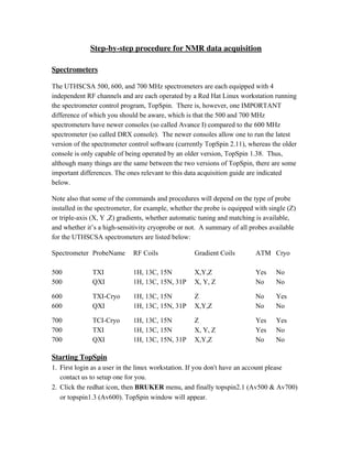
The UTHSCSA 500, 600, and 700 MHz spectrometers are each equipped with 4
independent RF channels and are each operated by a Red Hat Linux workstation running
the spectrometer control program, TopSpin. There is, however, one IMPORTANT
difference of which you should be aware, which is that the 500 and 700 MHz
spectrometers have newer consoles (so called Avance I) compared to the 600 MHz
spectrometer (so called DRX console). The newer consoles allow one to run the latest
version of the spectrometer control software (currently TopSpin 2.11), whereas the older
console is only capable of being operated by an older version, TopSpin 1.38. Thus,
although many things are the same between the two versions of TopSpin, there are some
important differences. The ones relevant to this data acquisition guide are indicated
below.
Note also that some of the commands and procedures will depend on the type of probe
installed in the spectrometer, for example, whether the probe is equipped with single (Z)
or triple-axis (X, Y ,Z) gradients, whether automatic tuning and matching is available,
and whether it’s a high-sensitivity cryoprobe or not. A summary of all probes available
for the UTHSCSA spectrometers are listed below:
Spectrometer ProbeName RF Coils Gradient Coils ATM Cryo
500 TXI 1H, 13C, 15N X,Y,Z Yes No
500 QXI 1H, 13C, 15N, 31P X, Y, Z No No
600 TXI-Cryo 1H, 13C, 15N Z No Yes
600 QXI 1H, 13C, 15N, 31P X,Y,Z No No
700 TCI-Cryo 1H, 13C, 15N Z Yes Yes
700 TXI 1H, 13C, 15N X, Y, Z Yes No
700 QXI 1H, 13C, 15N, 31P X,Y,Z No No
Starting TopSpin
1. First login as a user in the linux workstation. If you don't have an account please
contact us to setup one for you.
2. Click the redhat icon, then BRUKER menu, and finally topspin2.1 (Av500 & Av700)
or topspin1.3 (Av600). TopSpin window will appear.
2. Preparation for acquisition
1. Since some of the commands of TopSpin require a dataset, open a dataset first. You
can do this by clicking the Browser menu from the lefthand side panel and choosing
appropriate data set. Currently, all the users' datasets are stored in /avance5004, /
avance6003 and /avance7002 disks on the 500, 600 and 700 MHz spectrometers
respectively. If these data directories are not displayed (as will be the case for a first
time user), you can add them by right clicking and choosing “Add new data dir...”
menu. To open a data set listed in the browser double click or right click and choose
“display” (drag and drop has now been disabled).
2. Now the desired sample temperature can be set by typing edte at the command line.
Wait for the sample temperature to reach the desired value before proceeding to the
next step.
Inserting Sample
1. NMR tube containing sample should be held in a plastic spinner (use the blue color
spinner in 500 and 600 MHz spectrometers; use the white color spinner in 700 MHz
spectrometer). Hold the sample by the top, place sample tube in the spinner and the
spinner in the sample depth gauge. Push or pull the sample tube so that the depth of
the sample above and below the center line of the sample depth gauge is equal.
However, never exceed the lower limit (position of the adjustable white platform,
3. which should be at the line marked 5 mm 15mm) as this can damage the probe as
well as the sample, as the sample will rest on the tip of the tube, not the spinner. This
is important for all probes, but especially the cryoprobes installed on the 600 and
700MHz spectrometers.
2. Remove the black cap from the top of the magnet bore. Next, press the LIFT button in
upper left portion of the BSMS keyboard. Wait for the airflow (hissing sound that can
be heard). Then remove the depth gauge before inserting the sample and spinner into
the magnet. Pressing the LIFT button will toggle the air flow off and will drop the
sample tube gently to the magnet bore where it will be positioned at the top of the
probe.
Locking
3. Lock signal can be seen in the lock display window that can be opened by typing
lockdisp at the command line.
4. Enter lock at the command line and select appropriate solvent from the pop up solvent
table window (H20+D2O or CDCl3 etc) and wait for the “lock finished” message to
appear at the bottom of the topspin window. After that Lock On/Off LED will light on
the BSMS keyboard. DO NOT LOCK THE SPECROMETER USING ANY OTHER
METHOD. If the spectrometer fails to lock, this may indicate that your sample does
not include any deuterated solvent.
Tuning and Matching the Probe
The resonance frequency of the RF coils will vary depending on the content
(particularly, the salt content) of the individual NMR sample. Thus, it's necessary to
“Tune” the RF coil to the correct value to yield the correct resonant frequency for the
magnet field strength you are using. This is done by inserting the sample in the probe
and then by adjusting two variable capacitors, called “tune” and “match” on the probe
such that the reflected radio frequency power is minimized at the proper frequency.
Importantly, the higher frequency, the greater the degree to which the “tuning” of the
RF coil will depend on the content of the particular sample. This in practical terms
means that it is essentially always necessary to tune the RF coil for 1H, whereas it is
less important for lower frequency nuclei, such as 13C and 15N. Thus, in terms of
standard operating procedures, we recommend that you ALWAYS adjust the 1H
tuning, whereas adjustment of 13C and 15N tuning should be considered optional (and
in most cases, not necessary).
5. On probes equipped with automatic tuning and matching (ATM), this can be done
4. with the “atmm” command. Currently, the conventional TXI probe on the 500 and
conventional TXI and TCI cryoprobe on the 700 include ATM. Open an existing
dataset and then use the “edc” command to save it to a new name (such as tune1h).
Now type rpar Tuneh and press enter. In the acquisition window type atmm and
press enter. Click “optimize” at the top of the atmm menu bar and choose start. This
will enable tuning and matching of the probe for the selected channel (1H in this case).
Alternatively, do not click optimize and manually adjust with the displayed tuning and
matching buttons. Repeat this process for the all the desired channels (You will have
to setup separate experiments for this, for example using rpar Tunec and rpar
Tunen to tune either the 13C or 15N channels, respectively).
6. On probes without ATM, open an existing dataset and then use the “edc” command to
save to a new name (such as tuneh). Now, type rpar Tuneh and press enter. Then go
to the acquisition window by clicking acqu in the current datset menu bar or simply
type a at the command line. Now type wobb at the command line. Go to the magnet
and look for various screws underneath. These are color coded such that they match
the color on the plate of the probe where RF cables attach. On all probes, yellow
corresponds to 1H, red corresponds to 15N, and blue corresponds to 13C. Adjust
those screws using the tool (either attached to the probe by a flexible chain or a
separate tool, which we usually keep next to the magnet on the top of the preamp)
until you get good tuning and matching. After this type stop. To tune other nuclei,
such as 13C and 15N open an existing dataset and then use the “edc” command to
save to a new name (such as tunec or tunen). Now, type rpar Tunec or rpar Tunen
and press enter. Then go to the acquisition window and type wobb at the command
line and repeat the process as described above.
Examples of Wobble Curves with Different Tuning and Matching
bad matching and bad tuning bad matching and good tuning
5. good matching and bad tuning good matching and good tuning
Importantly, when manually tuning the cryoprobe on the 600 (which will always be
the case since it does not have an ATM device), you will need to type the command
crpoff prior to initiating the tuning procedure; once the tuning procedure is done, you
will need to type the command crpon (these commands switch the probe from the
normal situation where it uses internal cold preamplifiers to the standard warm
preamplifiers (which are needed for tuning) and then back again).
Shimming
Shimming is a process in which minor adjustments are made to the magnetic field
until uniform magnetic field is achieved around the sample. This is difficult to do
manually, but can be done using automatic procedures. Before shimming any sample,
read a recent stored shimfile for the current probe by typing rsh and choosing an
appropriate shim file from the list.
On the 500 and 700 MHz spectrometers there are two automated procedures possible,
named gradshim and topshim. Topshim is strongly recommended over Gradshim as
it's a newer procedure with a number of improvements relative to Gradshim. On the
600 MHz spectrometer, only Gradshim is available and therefore will have to be used.
7. To run Topshim, type topshim 1h 1d (or, if you have a Shigemi tube, topshim 1h 1d
shigemi). If your sample is 100% D2O or CDCl3 or any other deuterated solvent,
then use topshim 2h 1d. This procedure is entirely automated and will adjust the
shims along the Z-direction (these are the ones that vary most from sample to sample).
Typically, TopShim is complete within a minute, although it can be shorter or longer
than this depending on the initial homogeneity (generally, starting with poor shims
will cause TopShim to take longer to converge). Once Topshim is complete, click on
the autoshim button on the BSMS keypad, which will automatically optimize the most
sensitive Z- and X/Y shims in a continuous manner. Users may wish to save the
6. current shim set for future use; this may be done by typing wsh and by supplying a
descriptive filename.
NOTE, it is possible to use TopShim to shim in X, Y, and Z directions
simultaneously, using topshim 3d 1h. NOTE, however, this will only work on probes
with triple-axis gradient coils. which includes all of the UTHSCSA probes, except for
the 600 and 700 MHZ cyroprobes (which are equipped only with Z-gradient pulsed
field gradient coils).
8. To run Gradshim type gradshim. The first time gradshim is run there is a setup
process.
● Agree with the setup process and click "seen" to ignore all the error messages.
● For both 3D and 1D buttons (top of window) enter your username in the User field
and enter /opt/topspinx.x/ in the disk field.
● Create an iteration control file (the following is for 1D shimming).
● <edit> <iteration control> <new>
● Give the file a name, ie 1D_5steps
● Add the following 5 steps:
● step 1, lowz, size=18
● step 2, midz, size=18
● step 3, midz, size=18
● step 4, highz, size=18
● step 5, highz, size=18
● <save>
● The size is the length of the sample chamber. The units don't exactly
correspond to mm, but 18 is a good entry for an 18 mm chamber. If these sizes
are set too high, the procedure may fail to converge on a homogeneously
shimmed field.
● Thereafter, your iteration control file should be selected by default, but if not,
select it from the list. The * button expands the list of available iteration control
files.
● <Start gradient shimming>
● It should say that it will do 5 iterations. But, sometimes program exits after 1
iteration. If so, choosing the iteration control file from the list again will solve
this problem.
● A plot will be displayed of the frequency (as a measure of the field) over
vertical coordinates with 0 at the center of the sample. The size you have
selected is in a different color. The field is homogeneous when the central
7. colored part of the plot is vertical.
● You may have to repeat gradshim to get the field homogeneous. First delete the
previous plot window, else the new lines will be added to the old ones. If the
line has a hook on one end that can't be straightened, or appears to be unstable
in its effort to converge on a vertical line, your sample chamber may not be
centered properly.
9. Wait for the message “setsh finished” to appear at the bottom of the topspin main
window. This message indicates that gradshim is finished.
Setting up experiments
1. You need to create a new dataset before starting any experiment. To do this open an
existing dataset as described in the Step 1 of “Preparation for acquisition”. Now type
edc from the command line. In the edc display window which will pop up, type all the
necessary parameters like Name, Expno, Dir and User etc and then press OK. This will
take you to the new dataset you have created.
2. Next determine the 90 degree proton pulse at high power.
To do this on the 500 and 700 MHz spectrometer (running TopSpin 2.11),issue the
command pulsecal and wait. Calibrated pulselengths for a hard pulse and a soft pulse
will be shown in a new window. Note down these values.
The automated procedure, pulsecal is only available in the newer version of TopSpin.
Thus, the following manual procedure will have to be used on the 600. This procedure
can also be run on 500 & 700 and may be desirable if one suspects the values
determined by the pulsecal procedure are not accurate. To manually calibrate the 1H
pulse we use a one pulse experiment. To use this, create a new experiment (calib1h for
example) using edc command, and then type rpar calib1h on the command line. The
intensity of the resulting solvent peak will be maximum when the pulse length is
exactly 90 degree and the signal intensity will be minimum (null signal) when the
pulse length is equal to multiples of 180 degree (180, 360, 540, 720 etc). But, in
practice, due to radiation damping the solvent signal won't be null for 180 degree pulse
if your sample is in 90%H2O/10%D2O. Only, 360 degree pulse gives the null signal.
So, finding out the 360 degree pulse is widely recommended. Open the calib1h
dataset and set pl1 (power level for the hard 90 degree) as -3 dB (in 500 MHz & 600
MHz spectrometers) or +2.5 dB (in 700 MHz spectrometer). Set p1 as 1u and then
type “zgefp”. Type “apk” (automatic phase correction) to phase the spectrum. Zoom
in around the water signal using the mouse and the type dpl1 at the at the command
8. line. Now type “popt” at the command line and press enter. A window will pop up.
Enter the STARTVAL, ENDVAL and INC parameters for the parameter p1 (90
degree hard proton pulse). For example, enter 30 usec, 36 usec and 0.4 usec for
STARTVAL, ENDVAL and INC fields respectively. Then click the start optimize
button. After popt is finished you can see that solvent signal intensity will be plotted
as a function of p1 value. Find out the p1 value corresponding to 360 degree (p1 value
at which you see a null). From that value 90 degree pulse can be calculated. Readjust
the STARTVAL, ENDVAL, and INC values if you don't see any NULL.
Since all multiples of 360 degree pulses (720, 1080 degrees etc) give you a null signal
(see the sine wave diagram), beginners sometimes get confused in choosing the correct
null. This is especially true when you have high salt sample. So, use the following tip
to avoid this confusion. Calculate the 90 degree pulse from the value you got for 360
degree pulse. In the calib1h experiment set p1 to 90 degree pulse. Acquire the signal
(zg followed by efp or zgefp). Type apk to phase correct it. The signal should be a
maximum. Now set p1 to 360 degree pulse. Acquire the signal (do not phase correct
the signal). You should see a null signal. Finally, set p1 to 270 degree pulse. Acquire
the signal (Again, do not phase correct it). Now you should see a signal with negative
maximum. If you don't see the signal intensities as explained above then it is likely
that you are seeing a wrong null and pulse length calibrated for 90 degree is wrong.
3. To setup your experiment of interest, use edc to create a new data set and then use
rpar to read a standard parameter set for the experiment. If you wish to run 1D proton
spectrum then choose PROTON or any other suitable standard parameter set from the
list and click OK. Similarly, if you wish to run a 2D heteronuclear experiment like
HSQC, then choose a parameter set like HSQCETF3GPSI from the list and click OK.
This step will ensure that all the necessary standard parameters are copied for the
9. experiment. Please note that the standard parameter sets are named according to a
standard coding method (see the Pulprog.info in the /opt/topspinX.x/exp/stan/nmr/lists
/pp/ directory for a detailed explanation of the coding system).
4. Type edasp and check that the routings are OK. A typical routing setup for the
UTHSCSA spectrometers is shown below. Loading standard parameter sets will
ensure the correct edasp settings for you. Nevertheless, it is still a good idea to check
the edasp settings before you start any NMR experiment.
5. Issue the command “getprosol 1H <pulselength> <power>”. Substitute the values of
the proton hard pulse length and power level you got from step 2 above (for example,
getprosol 1H 8.0 2.0) here. All the other 1H pulses and their power levels (as well as
pulse times and power levels for other nuclei) will be calculated and stored in the
current dataset.
6. Now you have to set the carrier positions for each of the dimensions of your
experiment. These parameters determine the center of the spectrum in ppm and are set
by typing the commands o1p, o2p, and o3p. Common center positions in ppm for the
different nuclei are listed in the table below:
10. 1H H2O 4.706
1H amide 8.50
13C Calpha 53.5
13C Ca/Cb Center 46.0
13C Carbonyl 173.5
15N amide 118.0
As an example, if you wanted to setup a 3D HNCA experiment, you would type o1p
4.706, o2p 53.5, and 03p 118.0. Although these values should work for most
proteins, it may be desirable to optimize them (particularly, 15N carrier position for
example) for your individual protein.
7. After setting the center, you have to set the desired spectral width in units of ppm. You
can set these values by issuing eda command or clicking “AcquPars” menu. In the eda
window look for SW[PPM] parameter. If you do not see that then click the width
menu in the left hand side panel. Set the correct values for ALL dimensions . Typical
values for common experiments are listed in the table below:
Experiment Sweep Width/Spectral Width
1D 1H: 16ppm
1D 13C: 200ppm
2D H-N HSQC: 1H – 16ppm, 15N – 28 ppm
3D HNCA: 1H – 16ppm, 15N – 28 ppm, 13C – 24 ppm
3D HNCO: 1H – 16ppm, 15N – 28 ppm, 13C – 12 ppm
3D CBCA(CO)NH: 1H – 16ppm, 15N – 28 ppm, 13C – 60 ppm
3D HNCACB: 1H – 16ppm, 15N – 28 ppm, 13C – 60 ppm
etc
8. Change the number of sample points (TD) in each dimension if you are not satisfied
with the default values set by rpar command. Typically, TD is set to 16, 32 or 64k for
standard 1D experiments. In the multidimensional experiments TD for direct
dimension (usually proton) is set for 1k or 2k. Follow the table to get some idea about
the TD set for indirectly detected dimension.
Experiment Indirect dimension TD
2D-15N HSQC 15N 360–400
2D-13C HSQC 13C 240-320
2D-13C HSQC 13C determined by the
(Constant time version) decremental delay
3D HNCA 15N 64
11. 3D HNCA 13C 120-130
3D CBCA(CO)NH 15N 64
3D CBCA(CO)NH 13C 120-130
3D HCCH-TOCSY 1H 130-150
3D HCCH-TOCSY 13C 64-80
3D 15N NOESY 1H 220-280
3D 15N NOESY 15N 64-96
3D 13C NOESY 1H 220-280
3D 13C NOESY 13C 64-96
Graphical Representation of Acquisition Parameters
9. Change the number of scans (NS) & dummy scans (DS) if you need to. Increasing the
NS will improve the quality (Signal-to-Noise ratio) of the spectrum . But, the total
experiment time will also be increased. Typical 1D experiments can have NS of 1k or
2k. But, typical 2D experiments will be completed in an hour if you set the NS to 8
and TD to 360. But if you set NS to 32 then the same experiment will take 4 hrs to
complete. So, increase the number of scans only if needed. Also, note that NS should
ideally be an integral number of the longest phase cycle in the pulse program. For
example, if the longest phase cycle of the pulseprogram is 8 then you should set NS
to integral multiples 8. Use the command expt to determine the total time needed to
12. complete the experiment. During dummy scans, the actual experiment will be run but
no data will be acquired. This will help sample to reach a steady state or equilibrium.
For DS default value set by the rpar command should be sufficient.
10. The receiver gain is set by the parameter rg. Receiver gain is a very important
parameter to match the amplitude of the fid to the dynamic range of the digitizer. If the
FID is clipped at the top or bottom of the display then rg should be reduced. If the
gain is too low and not utilizing a suitable (25-40 %) part of the dynamic range of the
digitizer, it should be increased. Typically, the receiver gain is set automatically by the
rga command.
Effect of clipped fid as a result of RG set too high
11.Type zg to start the acquisition. You should see an FID in the acquisition window as
shown below