Download to read offline


![Introduction Small Model Great Recession Medium scale Conclusion
Borrowing constraint
Agents face borrowing constraint
˜ΘtE∗
t [Qt+1]Lt+1 ≥ (1 + R)Bt+1,
where
˜Θt ≡ Θt
E∗
t [Qt+1]
Q
ε
We allow leverage to respond to changes in the land price:
microfounded in simple moral hazard setting,
ε > 0 agrees with evidence in Mian and Sufi (2011) on US micro
data for the 2000s.](https://image.slidesharecdn.com/pintussudaturgutsndedallas28march2019-190329113926/75/Financial-Frictions-under-Learning-8-2048.jpg)

![Introduction Small Model Great Recession Medium scale Conclusion
FOCs
Borrowers ’ first-order conditions are
Ct : Λt = Ct − ψ
N1+χ
t
1 + χ
−σ
Nt : ψNχ+α+γ
t = (1 − α − γ)AKα
t Lγ
t
Lt+1 : TtQtΛt = βE∗
t [Tt+1Qt+1Λt+1] + βγE∗
t [Λt+1Yt+1/Lt+1]
+Φt
˜ΘtE∗
t [Qt+1],
Kt+1 : Λt = βE∗
t [Λt+1(αYt+1/Kt+1 + 1 − δ)]
Bt+1 : Λt = β(1 + R)E∗
t [Λt+1] + (1 + R)Φt](https://image.slidesharecdn.com/pintussudaturgutsndedallas28march2019-190329113926/75/Financial-Frictions-under-Learning-10-2048.jpg)
![Introduction Small Model Great Recession Medium scale Conclusion
REE
Linearized expectational system (in log levels):
Xt = AXt−1 + BE∗
t−1[Xt] + CE∗
t [Xt+1] + N + Dξt + Fψt,
Xt ≡ (ct, qt, λt, φt, bt, kt, θt, τt), ξt and ψt are innovations.
Under REE, E∗
t = Et and there exists a unique stationary
equilibrium
Xt = Mre
Xt−1 + Hre
+ Gre
ξt + Jre
ψt,
where Mre
and Hre
solve
M = [I8 − CM]
−1
[A + BM],
H = [I8 − CMre
]
−1
[BH + CH + N]](https://image.slidesharecdn.com/pintussudaturgutsndedallas28march2019-190329113926/75/Financial-Frictions-under-Learning-11-2048.jpg)
![Introduction Small Model Great Recession Medium scale Conclusion
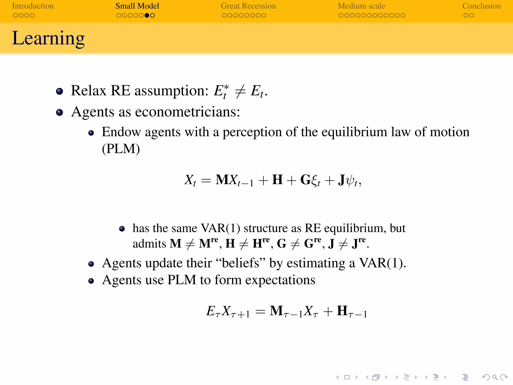
Learning
Agents as econometricians:
Actual low of motion becomes
[I8 −CMt−1]Xt = [A+BMt−2]Xt−1 +[BHt−2 +CHt−1 +N]+Dξt +Fψt
Assume recursive updating of the perceived law of motion
Ωt = Ωt−1 + ν(Xt − Ωt−1Zt−1)Zt−1R−1
t
Rt = Rt−1 + ν(Zt−1Zt−1 − Rt−1),
where Zt = [1, Xt ] and Ω = [H M]
OLS/RLS if νt = 1/t,
constant gain if νt = ν.
REE: perceived and actual laws of motions coincide.](https://image.slidesharecdn.com/pintussudaturgutsndedallas28march2019-190329113926/75/Financial-Frictions-under-Learning-13-2048.jpg)


![Introduction Small Model Great Recession Medium scale Conclusion
Estimation results Estimation
Results - Estimation
RE AL
Description Parameter Prior Posterior Mean Posterior Mean
Household Habit Persistency γh Beta 0.5122 [0.42,0.57] 0.5619 [0.55,0.57]
Entrepreneur Habit Persistency γe Beta 0.7924 [0.64,0.91] 0.6153 [0.61,0.62]
Investment Adjustment Cost Ω Gamma 0.1784 [0.15,0.21] 0.1595 [0.15,0.17]
Exo. Growth Rate gγ Gamma 0.3386 [0.27,0.45] 0.3817 [0.36,0.41]
SS Investment Specic Tech ¯λq Gamma 1.2919 [1.20,1.42] 1.2377 [1.21,1.28]
AR Patience ρa Beta 0.9340 [0.92,0.95] 0.9113 [0.90,0.92]
AR Perm. Technology ρz Beta 0.5560 [0.43,0.65] 0.4249 [0.40,0.47]
AR Trans. Technology ρvz Beta 0.3747 [0.08,0.61] 0.3141 [0.28,0.35]
AR Perm. Investment Tech ρq Beta 0.4810 [0.35,0.64] 0.6422 [0.60,0.67]
AR Trans. Investment Tech ρvq Beta 0.1523 [0.00,0.51] 0.2600 [0.23,0.29]
AR Land ρϕ Beta 1.0000 [1.00,1.00] 0.9997 [1.00,1.00]
AR Labor ρφ Beta 0.9987 [0.99,1.00] 0.9881 [0.99,0.99]
AR Collateral ρθ Beta 0.9879 [0.98,1.00] 0.9836 [0.98,0.98]
Std. Patience σa InvGamma 0.1404 [0.07,0.22] 0.1164 [0.08,0.14]
Std. Perm. Technology σz InvGamma 0.0038 [0.00,0.00] 0.0047 [0.00,0.00]
Std. Trans. Technology σvz InvGamma 0.0043 [0.00,0.00] 0.0037 [0.00,0.00]
Std. Perm. Investment Tech σq InvGamma 0.0042 [0.00,0.00] 0.0030 [0.00,0.00]
Std. Trans. Investment Tech σvq InvGamma 0.0022 [0.00,0.00] 0.0030 [0.00,0.00]
Std. Land σϕ InvGamma 0.0416 [0.04,0.05] 0.0451 [0.04,0.05]
Std. Labor σφ InvGamma 0.0069 [0.01,0.01] 0.0078 [0.01,0.01]
Std. Collateral σθ InvGamma 0.0109 [0.01,0.01] 0.0114 [0.01,0.01]
Gain g Gamma 0.0052 [0.01,0.01]
Log Marg. Likelihood 1940.3 1941.1
Pintus, Suda and Turgut (GRAPE) EXPECT 19.11.2018 15 / 25](https://image.slidesharecdn.com/pintussudaturgutsndedallas28march2019-190329113926/75/Financial-Frictions-under-Learning-35-2048.jpg)


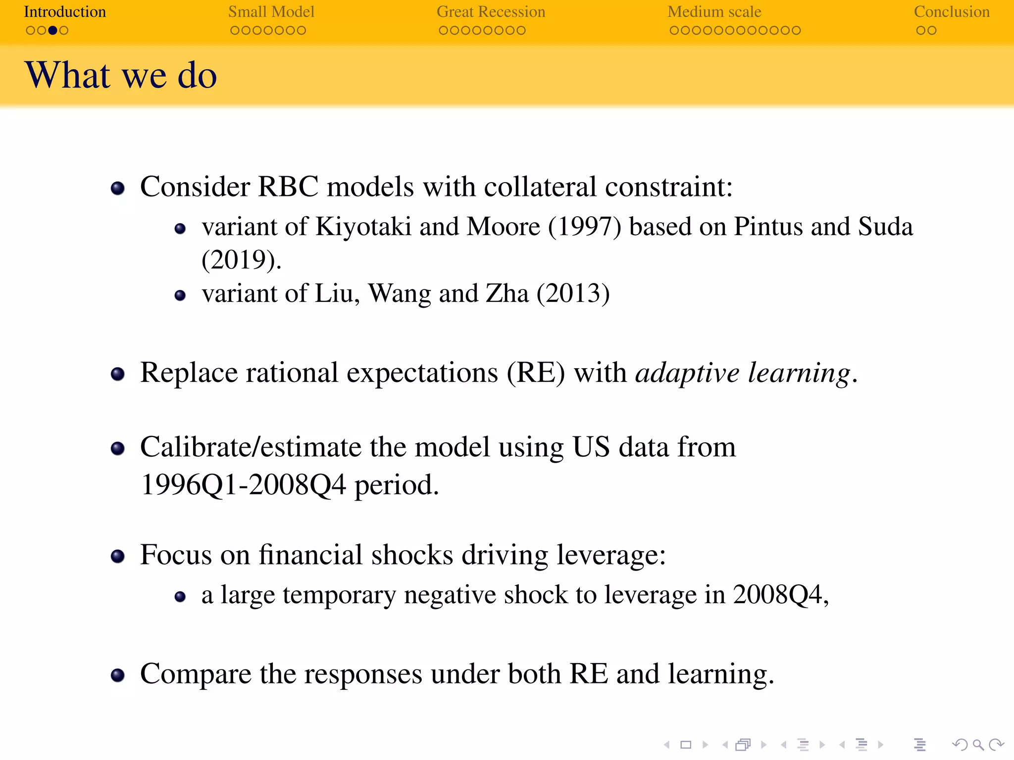
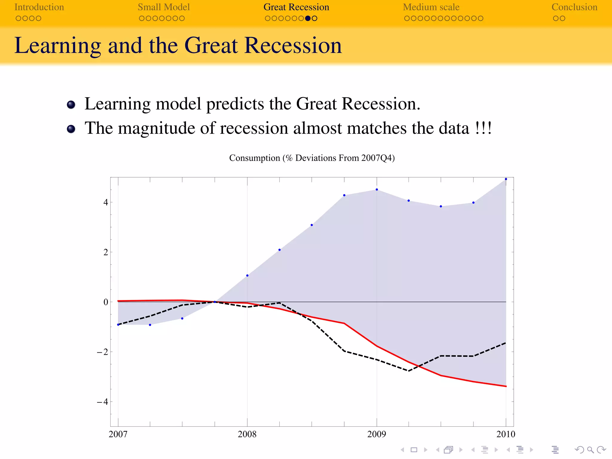
The document analyzes how adaptive learning may have contributed to the Great Recession, contrasting it with the rational expectations model. It presents a medium-scale model which demonstrates that agents' evolving perceptions of the economy can significantly influence financial behaviors and leverage, predicting a recession that aligns closely with observed data. The findings highlight time-varying impacts of shocks and the inadequacies of traditional rational expectations during financial crises.