Chapter 12analisis dec sensibilidad

Chapter 12 Projects Risk and Uncertainty

Sensitivity Analysis
12.1
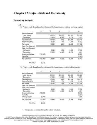
(a) Project cash flows based on the most-likely estimates: without working capital

0 1 2 3 4
Income Statement
Labor Savings $35,000 $35,000 $35,000 $35,000
Depreciation 21,600 34,560 20,736 6,221
Taxable Income $13,400 $440 $14,264 $28,779
Income Tax (40%) 5,360 176 5,706 11,512
Net Income $8,040 $264 $8,558 $17,268
Cash Flow Statement
Cash From Operation:
Net Income 8,040 264 8,558 17,268
Depreciation 21,600 34,560 20,736 6,221
Investment&Salvage (108,000) 30,000
Gains Tax (2,047)
Net Cash Flow (108,000) 29,640 34,824 29,294 51,442

PW (10%) = $4,870

(b) Project cash flows based on the most-likely estimates: with working capital

0 1 2 3 4
Income Statement
Labor Savings $35,000 $35,000 $35,000 $35,000
Depreciation 21,600 34,560 20,736 6,221
Taxable Income $13,400 $440 $14,264 $28,779
Income Tax (40%) 5,360 176 5,706 11,512
Net Income $8,040 $264 $8,558 $17,268
Cash Flow Statement
Net Income 8,040 264 8,558 17,268
Depreciation 21,600 34,560 20,736 6,221
Investment&Salvage (108,000) 30,000
Gains Tax (2,047)
Working Capital (5,000) 5,000
Net Cash Flow (113,000) 29,640 34,824 29,294 56,442

PW (10%) = $3,285

∴ The project is acceptable under either situation.

Contemporary Engineering Economics, Fourth Edition, By Chan S. Park. ISBN 0-13-187628-7.
© 2007 Pearson Education, Inc., Upper Saddle River, NJ. All rights reserved. This material is protected by Copyright and written permission should be
obtained from the publisher prior to any prohibited reproduction, storage in a retrieval system, or transmission in any form or by means, electronic, mechanical,
photocopying, recording, or likewise. For information regarding permission(s), write to: Rights and Permissions Department,
Pearson Education, Inc., Upper Saddle River, NJ 07458.

2

(c) Required annual savings (X):

0 1 2 3 4
Income Statement
Labor Savings $43,370 $43,370 $43,370 $43,370
Depreciation 21,600 34,560 20,736 6,221
Taxable Income $21,770 $8,810 $22,634 $37,149
Income Tax (40%) 8,708 3,524 9,053 14,860
Net Income $13,062 $5,286 $13,580 $22,289
Cash Flow Statement
Net Income 13,062 5,286 13,580 22,289
Depreciation 21,600 34,560 20,736 6,221
Investment & Salvage (108,000) 30,000
Gains Tax (2,047)
Net Cash Flow (108,000) 34,662 39,846 34,316 56,463

PW(18%) = $0

The required annual savings is $43,370.

12.2
• Project’s IRR if the investment is made now:

PW (i ) = −$500, 000 + $200, 000( P / A, i, 5) = 0

∴ i = 28.65%

• Let X denote the additional after-tax annual cash flow:
PW (28.65%) = −$500, 000 + X ( P / A, 28.65%, 4)( P / F , 28.65%,1) = 0

∴ X = $290, 240

12.3
(a) Economic building height

• 0% < i < 20% : The optimal building height is 5 Floors.
• 20% < i < 30% : The optimal building height is 2 Floors.


3

Ne t Ca sh F lo w s

n 2 F loors 3 F loors 4 F loors 5 F loors
0 ($500,000) ($750,000) ($1,250,000) ($2,000,000)
1 $199,100 $169,200 $149,200 $378,150
2 $199,100 $169,200 $149,200 $378,150
3 $199,100 $169,200 $149,200 $378,150
4 $199,100 $169,200 $149,200 $378,150
5 $799,100 $1,069,100 $2,149,200 $3,378,150
S e n sitivity An a lysis
P W (i) a s a F u n ctio n o f In te re st Ra te
B es t
i (% ) F loor P lan
5 $832,115 $687,643 $963,010 $1,987,770 5
6 $787,037 $635,190 $873,011 $1,834,680 5
7 $744,141 $585,370 $787,722 $1,689,448 5
8 $703,298 $538,023 $706,879 $1,551,593 5
9 $664,388 $493,002 $630,199 $1,420,666 5
10 $627,298 $450,168 $557,428 $1,296,250 5
11 $591,924 $409,393 $488,330 $1,177,957 5
12 $558,167 $370,556 $422,686 $1,065,427 5
13 $525,937 $333,545 $360,291 $958,321 5
14 $495,148 $298,257 $300,953 $856,326 5
15 $465,720 $264,594 $244,495 $759,148 5
16 $437,580 $232,465 $190,751 $666,513 5
17 $410,657 $201,784 $139,565 $578,166 5
18 $384,885 $172,472 $90,792 $493,867 5
19 $360,205 $144,454 $44,298 $413,393 5
20 $336,557 $117,661 ($46) $336,533 2
21 $313,889 $92,027 ($42,357) $263,091 2
22 $292,150 $67,490 ($82,746) $192,883 2
23 $271,292 $43,993 ($121,319) $125,737 2
24 $251,271 $21,482 ($158,173) $61,490 2
25 $232,044 ($95) ($193,399) ($9) 2
26 $213,572 ($20,784) ($227,084) ($58,903) 2
27 $195,817 ($40,632) ($259,308) ($115,327) 2
28 $178,745 ($59,679) ($290,148) ($169,407) 2
29 $162,323 ($77,967) ($319,674) ($221,261) 2
30 $146,519 ($95,532) ($347,955) ($271,002) 2

(b) Effects of overestimation on resale value:

Resale Present Worth as a Function of Number of Floors
value
2 3 4 5
Base $465, 720 $264,594 $244, 495 $759,148
10% error $435,890 $219,898 $145, 060 $609,995
Difference $29,831 $44, 696 $99, 435 $149,153


4

12.4 Note: In the problem statement, the current book value for the defender is
given as $13,000. This implies that the machine has been depreciated under the
alternative MACRS with half-year convention. In other words, the allowed
depreciation is based on a 10-year recovery period with straight-line method.
With the half-year convention mandated, the book value that should be used in
determining the gains tax for the defender (if sold now) is

Total depreciation = $1, 000 + $2, 000 + $2, 000 + $1, 000 = $6, 000
Book value = $20, 000 − $6, 000 = $14, 000
Taxable gain (loss) = $6, 000 − $14, 000 = ($8, 000)
Net proceeds from sale = $6, 000 + $8, 000 × 0.4 = $9, 200

Now the net proceeds from sale can be applied toward purchasing the new
machine. Thus, the net investment required for new machine will be only $2,800.
Note that, if you decide to retain the old machine, the current book value will be
$13,000 as you continue to depreciate the asset without any adjustment.

Comments: We will consider the various replacement problems in Chapter 14,
where the net proceeds from sale of the old machine is treated as an opportunity
cost of retaining the old machine, or simply the new investment required to keep
the old machine.

(a) Defender versus Challenger:

Keep the old machine
n 4 5 6 7 8 9 10
Financial Data 0 1 2 3 4 5 6
Depreciation $2,000 $2,000 $2,000 $2,000 $2,000 $2,000
Book value $13,000 $11,000 $9,000 $7,000 $5,000 $3,000 $1,000
Market value $1,000
Gain/loss
Removal cost 1,500
Operating cost 2,000 2,000 2,000 2,000 2,000 2,000
Cash Flow Statement
Removal ($900)
+(.4)*(Depreciation) 800 800 800 800 800 800
Net proceeds from sale 1,000
-(1-0.40)*(Operating cost) (1,200) (1,200) (1,200) (1,200) (1,200) (1,200)
Net Cash Flow $0 ($400) ($400) ($400) ($400) ($400) ($300)

PW (10%) = ($1,686) AE (10%) = ($387)


5

Buy a new machine

Financial Data n 0 1 2 3 4 5 6
Depreciation $2,400 $3,840 $2,304 $1,382 $1,382 $691
Book value $12,000 9600 5760 3456 2074 691 0
Market value 2000
Gain/loss 2000
Operating cost 1000 1000 1000 1000 1000 1000
Cash Flow Statement
Sale of old equipment 9,200
Investment (12,000)
+(.4)*(Depreciation) 960 1,536 922 553 553 276
-(1-0.40)*(Operating cost) (600) (600) (600) (600) (600) (600)
Net Cash Flow ($2,800) $360 $936 $322 ($47) ($47) $876

PW (10%) = ($1,024) AE (10%) = ($235)

∴ Incremental cash flows:

Net Cash Flow Incremental Cash flow
n New Machine Old Machine (new-old)
0 −$2,800 −$2,800
1 360 −400 760
2 936 −400 1, 336
3 322 −400 732
4 −47 −400 353
5 −47 −400 353
6 876 −300 1,176

IRR new−old = 18.32%, PW (10%) new−old = $669

∴ The defender should be replaced now.

(b) Sensitivity analysis: The answer remains unchanged. In fact, it (an increase in
O&M) will make the challenger more attractive.( IRR new−old = 24.26%, and
PW (10%) new−old = $1, 280 )

(c) Break-even trade-in value: Let X denote the minimum trade in value for the
old machine. Then, the net proceeds from sale of the old machine will be

Total depreciation = $6, 000
Book value = $14, 000
Salvage value = X
Taxable gain = X − $14, 000
Net proceeds = X − (0.40)( X − $14, 000)
= 0.6 X + $5, 600


6

To find the break-even trade-in value,

PW (10%)old = −$400( P / A,10%,5) − $300( P / F ,10%, 6) = −$1, 686
PW (10%) new = −[$12, 000 − (0.6 X + $5, 600)]
+$360( P / F ,10%,1) + + $877( P / F ,10%, 6)
= 0.6 X − $4, 624

Let PW (10%)old = PW (10%)new and solve for X .

∴ X = $4,897

12.5
(a) Total length of a new phone line - 5 miles:

• Option 1-Copper wire:

5 miles = 5 × 5,280 = 26,400 feet
First cost = (1,692 + 0.013 × 2,000) × 26,400 = $731,069 = $731, 069
Annual operating cost = $731,069(0.184) = $134,517

AEC (15%)1 = $731, 069( A / P,15%,30) + $34,517
∴
= $111,342

• Option 2-Fiber optics:

Cost of ribbon = $15,000/mile × 5miles = $75,000
Cost of terminators = $30,000 × 6 = $180,000
Cost of modulating system = ($12, 092 + $21, 217)(21)(2) = $1,398,978
Cost of repeater = $15,000 × 2 = $30,000
Total first cost = $75,000 + $180,000 + $1,398,978 + $30,000 = $1,683,978
Annual operating costs = $1, 398, 978(0.125) +$75, 000(0.178) = $188, 222

AEC (15%) 2 = $1, 683,978( A / P,15%,30) + $188, 222
∴
= $256, 470

∴ Select Option 1.


7

(b) Sensitivity Analysis

• Total length of phone lines -10 miles:

AEC (15%)1 = $491, 718
AEC (15%)2 = $471, 749

∴ Option 2 is the better choice.

• Total length of the phone lines - 25 miles:

AEC (15%)1 = $1, 229, 293
AEC (15%) 2 = $552,920

∴ Option 2 is the better choice.


8

12.6
(a) With infinite planning horizon: We assume that both machines will be available in the future with the same cost. (Select
Model A)

M ode l A

F i n a n c i a l D a ta
n 0 1 2 3 4 5 -7 8
D e p re c ia t io n $857 $1,469 $1,049 $749 $536 $268
B o o k va lu e $6,000 $5,143 $3,673 $2,624 $1,874 $1,339 $0
M a rk e t va lu e $500
G a in s / L o s s e s $500
O&M $700 $700 $700 $700 $700 $700

C a sh F l o w S ta te m e n t
In ve s t m e n t ($ 6 , 0 0 0 )
+ (. 3 0 )*(D e p re c ia t io n ) $257 $441 $315 $225 $161 $80
-(1 -0 . 3 0 )*(O & M ) ($ 4 9 0 ) ($ 4 9 0 ) ($ 4 9 0 ) ($ 4 9 0 ) ($ 4 9 0 ) ($ 4 9 0 )
N e t p ro c e e d s fro m s a le $350
N e t C a s h F lo w ($ 6 , 0 0 0 ) ($ 2 3 3 ) ($ 4 9 ) ($ 1 7 5 ) ($ 2 6 5 ) ($ 3 2 9 ) ($ 6 0 )

P W (1 0 % ) = ($ 7 , 1 5 2 ) A E C (1 0 % ) = $1,341

M ode l B

F i n a n c i a l D a ta
n 0 1 2 3 4 5 -7 8 9 10
D e p re c ia t io n $1,215 $2,082 $1,487 $1,062 $759 $379
B o o k va lu e $8,500 $7,285 $5,204 $3,717 $2,655 $1,896 ($ 0 ) ($ 0 ) ($ 0 )
M a rk e t va lu e $1,000
G a in s / L o s s e s $1,000
O&M $520 $520 $520 $520 $520 $520 $520 $520

C a sh F l o w S ta te m e n t
In ve s t m e n t ($ 8 , 5 0 0 )
+ (. 3 0 )*(D e p re c ia t io n ) $364 $624 $446 $318 $228 $114 $0 $0
-(1 -0 . 3 0 )*(O & M ) ($ 3 6 4 ) ($ 3 6 4 ) ($ 3 6 4 ) ($ 3 6 4 ) ($ 3 6 4 ) ($ 3 6 4 ) ($ 3 6 4 ) ($ 3 6 4 )
N e t p ro c e e d s fro m s a le $700
N e t C a s h F lo w ($ 8 , 5 0 0 ) $0 $260 $82 ($ 4 6 ) ($ 1 3 6 ) ($ 2 5 0 ) ($ 3 6 4 ) $336

P W (1 0 % ) = ($ 8 , 6 2 7 ) A E C (1 0 % ) = $1,404


9

(b) Break-even annual O&M costs for machine A: Let X denotes a before-tax
annual operating cost for model.

PW (10%) A = −$6, 000 + ($257 − 0.7 X )( P / F ,10%,1) +
+ ($458 − 0.7 X )( P / F ,10%,8)
= −$4,526 − 3.734 X
AEC (10%) A = $849 + 0.7 X

Let AEC (10%) A = AEC (10%) B , and solve for X.

$849 + 0.7 X = $1, 404

∴ X = $793 per year

(c) With a shorter service life:

Net Cash Flow
n
Model A Model B
0 -$6,000 -$8,500
1 -233 0
2 -49 260
3 -175 82
4 -265 -46
5 2,172 2,883
PW(10%) -$5,216 -$6,464

∴ Model A is still preferred over Model B.


10

12.7 Assuming that all old looms were fully depreciated
(a)
• Project cash flows: Alternative 1

Alternative 1

Financial Data
n 0 1 2 3 4 5 5 7 8
Depreciation $306,669 $525,564 $375,342 $268,040 $191,641 $191,426 $191,641 $95,713
Book value $2,146,036 1,839,367 1,313,803 938,462 670,422 478,781 287,354 95,713 0
Market value 169,000
Gain/Loss 169,000
Annual sales 7,915,748 7,915,748 7,915,748 7,915,748 7,915,748 7,915,748 7,915,748 7,915,748
Annual labor cost 261,040 261,040 261,040 261,040 261,040 261,040 261,040 261,040
Annual O&M cost 1,092,000 1,092,000 1,092,000 1,092,000 1,092,000 1,092,000 1,092,000 1,092,000

Cash Flow Statement
Investment ($2,108,836)
+(0.40)*Dn 122,667 210,226 150,137 107,216 76,656 76,571 76,656 38,285
+(0.60)*Sales 4,749,449 4,749,449 4,749,449 4,749,449 4,749,449 4,749,449 4,749,449 4,749,449
-(0.60)*Labor (156,624) (156,624) (156,624) (156,624) (156,624) (156,624) (156,624) (156,624)
-(0.60)*O&M (655,200) (655,200) (655,200) (655,200) (655,200) (655,200) (655,200) (655,200)

Net Cash Flow ($2,108,836) $4,060,292 $4,147,850 $4,087,761 $4,044,841 $4,014,281 $4,014,195 $4,014,281 $4,077,310

PW (18%) = $14,471,800 AE (18%) = $3,549,127

Note: Cost basis for the new looms = $ 2,119,170 + $ 26,866 = $ 2,146,036
Net investment required = Cost basis - Net proceeds from sale of the old looms
= $ 2,146,036 - $ 62,000 (1-0.40) = $ 2,108,836


11

• Project cash flows: Alternative 2

Alternative 2

Financial Data
n 0 1 2 3 4 5 5 7
Depreciation $160,083 $274,347 $195,930 $139,918 $100,038 $99,926 $100,038
Book value $1,120,242 960,159 685,812 489,882 349,964 249,926 150,000 49,963
Market value
Gain/Loss
Annual sales 7,455,084 7,455,084 7,455,084 7,455,084 7,455,084 7,455,084 7,455,084
Annual labor cost 422,080 422,080 422,080 422,080 422,080 422,080 422,080
Annual O&M cost 1,560,000 1,560,000 1,560,000 1,560,000 1,560,000 1,560,000 1,560,000

Cash Flow Statement
Investment ($1,083,042)
+(0.40)*Dn 64,033 109,739 78,372 55,967 40,015 39,970 40,015
+(0.60)*Sales 4,473,050 4,473,050 4,473,050 4,473,050 4,473,050 4,473,050 4,473,050
-(0.60)*Labor (253,248) (253,248) (253,248) (253,248) (253,248) (253,248) (253,248)
-(0.60)*O&M (936,000) (936,000) (936,000) (936,000) (936,000) (936,000) (936,000)
Net proceeds from sale

Net Cash Flow ($1,083,042) $3,347,835 $3,393,541 $3,362,175 $3,339,770 $3,323,817 $3,323,773 $3,323,817

PW (18%) = $12,575,319 AE (18%) = $3,084,026

Note: Cost basis for the new looms = $ 1,071,240 + $ 49,002 = $ 1,120,242
Net investment required = Cost basis - Net proceeds from sale of the old looms
= $ 1,120,242 - $ 62,000 (1-0.40) = $ 1,083,042


12

(b) Sensitivity graph

Sensitivity Graph

$25,000,000

Sales $20,000,000
Labor
O&M $15,000,000

N PW
MARR
$10,000,000

$5,000,000

$0
-30% -20% -10% 0% 10% 20% 30%
% Change

12.8 Sensitivity graph

$2,000,000
$1,800,000 V = 6000

$1,600,000
$1,400,000 V = 5000
$1,200,000
NPW ($)

$1,000,000 V = 4000
$800,000
V = 3000
$600,000
$400,000 V = 2000
$200,000 V = 1000
$0
20 25 30 35 40 45
Sales Price (X)


13

12.9
• AEC(10%)s for 200 shift:

AEC (10%) Electric = $38, 058( A / P,10%, 7) = $7,817
AEC (10%) LPG = $69,345( A / P,10%, 7) = $14, 244
AEC (10%)Gasoline = $54,971( A / P,10%, 7) = $11, 280
AEC (10%) Diesel = $49,994( A / P,10%, 7) = $10, 269

0 1 2 3 4 5 6 7
Electric Power
O&M ($2,025) ($2,025) ($2,025) ($2,025) ($2,025) ($2,025) ($2,025)
Initial cost ($29,739)
Salvage $3,000
Net cash flow ($29,739) ($2,025) ($2,025) ($2,025) ($2,025) ($2,025) ($2,025) $975
PW(10%) = ($38,058)

LPG
O&M ($10,100) ($10,100) ($10,100) ($10,100) ($10,100) ($10,100) ($10,100)
Salvage $2,000
Net cash flow ($21,200) ($10,100) ($10,100) ($10,100) ($10,100) ($10,100) ($10,100) ($8,100)
PW(10%) = ($69,345)

Gasoline
O&M ($7,372) ($7,372) ($7,372) ($7,372) ($7,372) ($7,372) ($7,372)
Salvage $2,000
Net cash flow ($20,107) ($7,372) ($7,372) ($7,372) ($7,372) ($7,372) ($7,372) ($5,372)
PW(10%) = ($54,971)

Diesel Fuel
O&M ($5,928) ($5,928) ($5,928) ($5,928) ($5,928) ($5,928) ($5,928)
Salvage $2,200
Net cash flow ($22,263) ($5,928) ($5,928) ($5,928) ($5,928) ($5,928) ($5,928) ($3,728)
PW(10%) = ($49,994)


14

• AEC(10%)s for 260 shift:
AEC (10%) Electric = $8, 275
AEC (10%) LPG = $16,974
AEC (10%)Gasoline = $13, 203
AEC (10%) Diesel = $11, 748

• Sensitivity graph: PW cost as a function of number of shifts

Electric P ower
LP G
Gasoline
$ 9 0 ,0 0 0
Diesel F uel

$ 8 0 ,0 0 0
$ 7 0 ,0 0 0
$ 6 0 ,0 0 0
$ 5 0 ,0 0 0
$ 4 0 ,0 0 0
$ 3 0 ,0 0 0
200 260 Shift

Break-Even Analysis
12.10
• PW of net investment:

P0 = −$2, 200, 000 − $600, 000 − $400, 000 = −$3, 200, 000

• PW of after-tax revenue:

P = −$4, 000(365) X (1 − 0.31)( P / A,10%, 25)
1

= $9,144, 210 X

• PW of after-tax operating costs:


15

P2 = −($230, 000 + $170, 000 X )(1 − 0.31)( P / A,10%, 25)
= −$1, 440,526 − 1, 064, 737 X

• PW of tax credit (shield) on depreciation:
Depreciation Combined
n
Building Furniture Tax savings
1 $54,060 $57,143 $111,203(0.31) = $34,473
2 56,410 97,959 154,369(0.31) = 52,018
3 56,410 69,971 126,381(0.31) = 39,178
4 56,410 49,979 106,389(0.31) = 32,981
5 56,410 35,699 92,109(0.31) = 28,554
6 56,410 35,699 92,109(0.31) = 28,554
7 56,410 35,699 92,109(0.31) = 28,554
8 56,410 17,850 74,260(0.31) = 23,021
9-24 56,410 0 56,410(0.31) = 17,487
25 54,060 0 54,060(0.31) = 16,759

P3 = $34, 473( P / F ,10%,1) + $52, 018( P / F ,10%, 2)
+ + $16, 759( P / F ,10%, 25)
= $250,902

• PW of net proceeds from sale:
Property Cost basis Salvage Book value Gains Gains
(asset) value (losses) Taxes
Furniture $400,000 $0 $0 $0 $0
Building 2,200,000 0 794,450 (794,450) (246,280)
Land 600,000 2,031,813 600,000 1,431,813 443,862

Net proceeds from sale = $2, 031,813 + $246, 280 − $443,862
= $1,834, 231
P4 = $1,834, 231( P / F ,10%, 25)
= $169, 292


16

PW (10%) = P0 + P + P2 + P3 + P4
1

= −$4, 220,332 + 8, 079, 473 X
=0

X = 52.24%

12.11 Useful life of the old bulb:

14, 600 /(19 × 365) = 2.1 years

For computational simplicity, let’s assume the useful life of 2 years for the old
bulb. Then, the new bulb will last 4 years. Let X denote the price for the new
light bulb. With an analysis period of 4 years, we can compute the equivalent
present worth cost for each option as follows:

PW (15%)old = (1 − 0.40)[$45.90 + $45.90( P / F ,15%, 2)]
= $65.23
PW (15%)new = (1 − 0.40)( X + $16)

The break-even price for the new bulb will be

0.6 X + 9.6 = $65.23

X = $92.72

∴ Since the new light bulb costs only $60, it is a good bargain.

12.12
• PW of net investment:
P0 = −$250, 000

• PW of after-tax rental revenue:
P = X (1 − 0.30)( P / A,15%, 20)
1

= $4.3815 X

• PW of after-tax operation costs:
P2 = −(1 − 0.30)$12, 000( P / A,15%, 20)
= −$52,578


17

• PW of tax credit (shield) on depreciation: (In this problem, we assume that the
purchasing cost of $250,000 does not include any land value. Therefore, the
entire purchasing cost will be the cost basis for depreciation purpose.)

Depreciation Combined
n Building Tax savings
1 $6,143 $6,143(0.30) = $1,843
2-19 6,410 6,410(0.30) = 1,923
20 6,143 6,143(0.30) = 1,843

P3 = $1,843( P / F ,15%,1) + $1,923( P / A,15%,19)( P / F ,15%,1)
+$1,843( P / F ,15%, 20)
= $11,962

• PW of net proceeds from sale:
Total depreciation = $127, 666
Book value = $250, 000 − $127, 666 = $122, 334
Salvage value = $250, 000(1.05) 20 = $663,324
Taxable gain = $663, 324 − $122, 334 = $540, 990
Gains tax = $540, 990(0.30) = $162, 297
Net proceeds from sale = $663, 324 − $162, 297 = $501, 027

P4 = $501, 027( P / F ,15%, 20)
= $30, 613

• The break-even rental:
PW (10%) = P0 + P + P2 + P3 + P4
1

= −$260, 003 + 4.3815 X
=0

∴ X = $59, 341


18

12.13 Let X denotes the additional annual revenue (above $16,000) for model A that
is required to breakeven.

• Generalized cash flow for model A:
Cash flow End of Year
elements 0 1 2 3 4 5 6
Investment ($80,000)
Net proceeds 12,000
$9,600 $9,600 $9,600 $9,600 $9,600 $9,600
+0.6Rn
+0.6X +0.6X +0.6X +0.6X +0.6X +0.6X
+0.4Dn $6,400 $10,240 $6,144 $3,686 $3,686 $1,843
-(0.6)O&M ($13,200) ($13,200) ($13,200) ($13,200) ($13,200) ($13,200)
$2,800 $6,640 $2,544 $86 $86 $10,234
Net cash flow ($80,000)
+0.6X +0.6X +0.6X +0.6X +0.6X +0.6X

PW (20%) A = −$68, 077 + 1.9953 X

• Generalized cash flow for model B:
Cash flow End of Year
elements 0 1 2 3 4 5 6
Investment ($52,000)
Net proceeds 9000
+0.6Rn $0 $0 $0 $0 $0 $0
+0.4Dn $4,160 $6,656 $3,994 $2,396 $2,396 $1,198
-(0.6)O&M ($10,200) ($10,200) ($10,200) ($10,200) ($10,200) ($10,200)
Net cash flow ($52,000) ($6,040) ($3,544) ($6,206) ($7,804) ($7,804) ($2)

PW (20%) B = −$69,985

• By letting PW (20%) A = PW (20%) B
−$68, 077 + 1.9953 X = −$69,985
X = −$957

∴ The required break-even annual revenue for model A is then

$16,000 + X = $15,043

12.14 Let X denote the number of copies to breakeven.

• A/T annual revenue = (0.6)[$0.05 + ($0.25 − $0.05)] X = 0.15X


19

• A/T O&M cost = −(0.60)[$300, 000(12) + $0.10 X ] = $2,160, 000 + 0.06 X

Depreciation tax credit = (0.40)[$85, 714( P / F ,13%,1) +
+$26, 775( P / F ,13%,8)]( A / P,13%,10)
= $29, 285
CR (13%) = ($600, 000 − $60, 000)( A / P,13%,10) + (0.15)$60, 000
= $107,316
AE (13%) = 0.15 X − $2,160, 000 − 0.06 X + $29, 285 − $107,316
= 0.09 X − $2, 238, 031 = 0

∴ X = 24,867, 011 copies per year or 82,890 copies per day

Probabilistic Analysis
12.15
PW (12%)light = −$8, 000, 000 + $1,300, 000( P / A,12%,3)
= −$4,800, 000
PW (12%)moderate = −$8, 000, 000 + $2,500, 000( P / A,12%, 4)
= −$406, 627
PW (12%) high = −$8, 000, 000 + $4, 000, 000( P / A,12%, 4)
= $4,149, 000
E[ PW (12%)] = −$4,800, 000(0.20) − $406, 627(0.40)
+$4,149, 000(0.40)
= $536,947

∴ Since E[ PW ] is positive, it is good to invest.

12.16
(a) The PW distribution for project 1:

Event (x,y) Joint Probability PW (10%)
($20,$10) 0.24 $8,000
($20,$20) 0.36 $16,000
($40,$10) 0.16 $32,000
($40,$20) 0.24 $64,000


20

(b) The mean and variance of the NPW for Project 1:

E[ PW (10%)]1 = $8, 000(0.24) + $16, 000(0.36) + $32, 000(0.16)
+$64, 000(0.24)
= $28,160
Var[ PW (10%)]1 = (8, 000 − 28,160) 2 (0.24) + (16, 000 − 28,160) 2 (0.36)
+(32, 000 − 28,160) 2 (0.16) + (64, 000 − 28,160)2 (0.24)
= 461, 414, 400

(c) The mean and variance of the NPW for Project 2:

E[ PW (10%)]2 = $8, 000(0.24) + $16, 000(0.20) + $32, 000(0.36)
+$64, 000(0.20)
= $32, 000
Var[ PW (10%)]2 = (8, 000 − 32, 000)2 (0.24) + (16, 000 − 32, 000)2 (0.20)
+ (32, 000 − 32, 000) 2 (0.36) + (64, 000 − 32, 000) 2 (0.20)
= 394, 240, 000
(d) Project 2 is preferred over project 1 because its mean is greater than that of
project 1 but its variance is smaller than that of project 1.

12.17

(a) Expected value criterion: Assume that the opportunity cost rate is 7.5%.

• Option 1:
E[ R ]1 = $2, 450(0.25) + $2, 000(0.45) + $1, 675(0.30)
−$150( F / P, 7.5%,1)
= $1,854

• Option 2:
E[ R]2 = $25, 000(0.075) = $1,875

∴ Option 2 is the better choice based on the principle of the expected value
maximization.

(c) Here we are looking for the value of perfect information. If we know for sure
that the bond yield would be $2,450, then our strategy would be to purchase
the bond. In the absence of this perfect information, Option 2 was the better
strategy. In terms of regret not selecting Option 1 is


21

$2,450(P/F, 7.5%, 1) - $1,875 = $414

If we know for sure that the bond yield would be either $2,000 or $1,675,
clearly we do not invest in bond, so there will be no regret. Since there is
only a 25% chance that the bond yield will be $2,450, we should not
solicit professional advice at any expense higher than (0.25)($414) = $104.

12.18 Let X denote the annual revenue in constant dollars and Y the general inflation
during the first year. Then Z is defined as (1 + Y ).

(a) NPW as functions of X and Z:
End of Period
Cash elements
0 1 2
Investment -$9,000
Salvage value 4, 000Z 2
Gains tax -( 4, 000Z 2 -5,200)(0.40)
(0.4) Dn 1,200 800
(0.6) Rn 0.6ZX 0.6 Z 2 X
working capital -2,000 2,000(1-Z) 2,000Z
3,200-2,000Z 2,400 Z 2 +3,000
Net cash flow -$11,000
+0.6ZX +0.6 Z 2 X+2,000Z

Note that the market interest rate is a random variable as the general inflation
rate becomes a random variable. There are nine joint events for X and Y. For a
joint event where x = 10, 000 and y = 0.05 (or z = 1.05 ), we first calculate the
market interest rate and then evaluate the PW function at this market interest
rate.
i = i '+ f + i ' f
= 0.10 + 0.05 + (0.1)(0.05)
= 15.5%

PW (15.5%) = −$11, 000 + [3, 200 − 2, 000(1.05)
+0.6(10, 000)(1.05)]( P / F ,15.5%,1) + [2, 400(1.05) 2
+3, 000 + 0.6(10, 000)(1.05) 2 + 2, 000(1.05)]( P / F ,15.5%, 2)
= $6,172

You repeat the process for the remaining joint events.


22

(b) Mean and variance calculation:

Event No. X Z A0 A1 A2 PW(15.5%)
1 $ 10,000 1.03 ($11,000) $7,320 $13,972 $5,811
2 $ 10,000 1.05 ($11,000) $7,400 $14,361 $6,172
3 $ 10,000 1.07 ($11,000) $7,480 $14,757 $6,538
4 $ 20,000 1.03 ($11,000) $13,500 $20,337 $15,933
5 $ 20,000 1.05 ($11,000) $13,700 $20,976 $16,585
6 $ 20,000 1.07 ($11,000) $13,900 $21,627 $17,246
7 $ 30,000 1.03 ($11,000) $19,680 $26,702 $26,055
8 $ 30,000 1.05 ($11,000) $20,000 $27,591 $26,999
9 $ 30,000 1.07 ($11,000) $20,320 $28,496 $27,954

Weighted Deviation Weighted
Event No. PW(15.5%) P(x) P(z) P(x,z) PW(15.5%) Deviation
1 $5,811 0.3 0.35 0.105 $610 153,014,104 16,066,481
2 $6,172 0.3 0.5 0.15 $926 38,094,719 5,714,208
3 $6,538 0.3 0.25 0.075 $490 42,749,655 3,206,224
4 $15,933 0.4 0.35 0.14 $2,231 253,864,423 35,541,019
5 $16,585 0.4 0.5 0.2 $3,317 275,072,678 55,014,536
6 $17,246 0.4 0.25 0.1 $1,725 297,429,425 29,742,942
7 $26,055 0.3 0.35 0.105 $2,736 67,881,135 71,282,519
8 $26,999 0.3 0.5 0.15 $4,050 728,921,068 109,338,160
9 $27,954 0.3 0.25 0.075 $2,097 781,424,027 58,606,802
E[PW]= $18,181 Var[PW] = 384,512,892

Comparing Risky Projects
12.19
(a)
E[ PW ]1 = ($2, 000)(0.20) + ($3, 000)(0.60) + ($3,500)(0.20) − $1, 000
= $1,900
E[ PW ]2 = ($1, 000)(0.30) + ($2,500)(0.40) + ($4,500)(0.30) − $800
= $1,850

∴ Project 1 is preferred over Project 2.


23

(b)
Var[ PW ]1 = (2, 000 − 1,900) 2 (0.20) + (3, 000 − 1,900) 2 (0.60)
+ (3,500 − 1,900) 2 (0.20)
= 1, 240, 000
Var[ PW ]2 = (1, 000 − 1,850) 2 (0.30) + (2,500 − 1,850) 2 (0.40)
+ (4,500 − 1,850) 2 (0.30)
= 2, 492,500

∴ Project 1 is still preferred, as we have Var1 < Var2 and E1 > E2 .

12.20
(a) Mean and variance calculations:

E[ PW ]1 = ($100, 000)(0.20) + ($50, 000)(0.40) + (0)(0.40)
= $40, 000
E[ PW ]2 = ($40, 000)(0.30) + ($10, 000)(0.40) + (−$10, 000)(0.30)
= $13, 000
Var[ PW ]1 = (100, 000 − 40, 000) 2 (0.20) + (50, 000 − 40, 000) 2 (0.40)
+ (0 − 40, 000) 2 (0.40)
= 1, 400, 000, 000
Var[ PW ]2 = (40, 000 − 13, 000) 2 (0.30) + (10, 000 − 13, 000) 2 (0.40)
+ (−10, 000 − 13, 000) 2 (0.30)
= 381, 000, 000

It is not a clear case, because E1 > E2 but also Var1 > Var2 .If she makes
decision solely based on the principle of maximization of expected value, she
may prefer contract A.

(b) Assuming that both contracts are statistically independent form each other,

Joint event ( PWA > PWB ) Joint Probability
($100,000,$40,000) (0.20)(0.30) = 0.06
($100,000,$10,000) (0.20)(0.40) = 0.08
($100,000,-$10,000) (0.20)(0.30) = 0.06
($50,000,$40,000) (0.40)(0.30) = 0.12
($50,000,$10,000) (0.40)(0.40) = 0.16
($50,000,-$10,000) (0.40)(0.30) = 0.12
($0,-$10,000) (0.40)(0.30) = 0.12
Σ = 0.72

24

12.21
(a)
• Machine A:
CR(10%) A = ($60, 000 − $22, 000)( A / P,10%, 6) + (0.10)($22, 000)
= $10,924
E[ AE (10%)]A = ($5, 000)(0.20) + ($8, 000)(0.30)
+($10, 000)(0.30) + ($12, 000)(0.20) + $10,924
= $19, 725
Var[ AE (10%)]A = (15,924 − 19, 725) 2 (0.20) + (18,924 − 19, 725) 2 (0.30)
+(20,924 − 19, 725) 2 (0.30) + (22,924 − 19, 725) 2 (0.20)
= 5,560, 000

• Machine B:
CR(10%) B = $35, 000( A / P,10%, 4)
= $11, 042
E[ AE (10%)]B = ($8, 000)(0.10) + ($10, 000)(0.30)
+ ($12, 000)(0.40) + ($14, 000)(0.20) + $11, 042
= $22, 442
Var[ AE (10%)]B = (19, 042 − 22, 442)2 (0.10) + (21, 042 − 22, 442) 2 (0.30)
+ (23, 042 − 22, 442) 2 (0.40) + (25, 042 − 22, 442) 2 (0.20)
= 3, 240, 000

(b) Prob[ AE (10%) A > AE (10%) B ] :

Joint event Joint
(O&M A ,O&M B ) ( AE A > AEB ) Probability
($10,000, $8,000) ($20,924, $19,042) (0.30)(0.10) = 0.03
($12,000, $8,000) ($22,924, $19,042) (0.20)(0.10) = 0.02
($12,000, $10,000) ($22,924, $21,042) (0.20)(0.30) = 0.06
Σ = 0.11

12.22
(a) Mean and variance calculation (Note: For a random variable Y, which can be
expressed as a linear function of another random variable X (say, Y = aX ,
where a is a constant) the variance of Y can be calculated as a function of
variance of X, Var[Y ] = a 2Var[ X ] .


25

E[ PW ]A = −$5, 000 + $4, 000( P / A,15%, 2)
= $1,502.84
E[ PW ]B = −$10, 000 + $6, 000( P / F ,15%,1) + $8, 000( P / F ,15%, 2)
= $1, 266.54
V [ PW ]A = 1, 0002 + ( P / F ,15%,1) 21, 0002 + ( P / F ,15%, 2) 21,5002
= 3, 042,588
V [ PW ]B = 2, 0002 + ( P / F ,15%,1) 21,5002 + ( P / F ,15%, 2)2 2, 0002
= 7,988,336

(b) Comparing risky projects

Project A Project B
E[ PW ] $1,503 $1,267
V [ PW ] 3,042,588 7,988,336

∴ Project A is preferred.

Decision Tree Analysis
12.23
(a) Let’s define the symbols:

P: Party is taking place
NP: No party is planned
TP: Tipster says “P”
TNP: Tipster says “NP”

Then,

P(NP ∩ TP) P(TP) = P(NP) P(TP NP)
= (0.4)(0.2) = 0.08

(b)
• Optimal decision without sample information:

EMV = (0.6)(100) + (0.4)(−50) = 40 points

∴ Raid the dormitories.


26

• Joint probabilities:

P (P ∩ TP) = P(P) P(TP / P) = (0.60)(0.40) = 0.24
P (P ∩ TNP) = P(P) P(TNP / P) = (0.60)(0.60) = 0.36
P (NP ∩ TP) = P (NP) P(TP / NP) = (0.40)(0.20) = 0.08
P (NP ∩ TNP) = P (NP) P (TNP / NP) = (0.40)(0.80) = 0.32

• Marginal probabilities:

P(TP) = P(P ∩ TP) + P(NP ∩ TP)
= 0.24 + 0.08 = 0.32
P(TNP) = P(P ∩ TNP) + P(NP ∩ TNP)
= 0.36 + 0.32 = 0.68

Tipster says Marginal
State of Nature
P NP Probability
P 0.24 0.36 0.6
Actual
NP 0.08 0.32 0.4
Marginal Probability 0.32 0.68 1

• Revised probabilities after receiving the tips:

P (P ∩ TP) 0.24
P(P/TP) = = = 0.75
P(TP) 0.32
P (NP ∩ TP) 0.08
P (NP/TP) = = = 0.25
P(TP) 0.32
P (P ∩ TNP) 0.36
P(P/TNP) = = = 0.5294
P(TNP) 0.68
P (NP ∩ TNP) 0.32
P(NP/TNP) = = = 0.4706
P(TNP) 0.68

• Optimal decision after receiving the tips: The tipster’s information has no
value, even though it costs nothing. Do not reply on the tips.


27

* Decision Tree

40 0.6 100

40 R
0.4 -50
-6 -10
NR 0.6
Do not take tips
40 0.4 0
62.5
0.75 100
62.5
Take tips R 0.25 -50
-7.5 -10
39.93 0.32 NR 0.75
TP 0
0.25
0.68 29.41 100
29.41 0.529
TNP R
0.471 -50
-5.3
NR -10
0529
0.471 0

(c) EVPI = 60 - 40 = 20

Comments: Note that if a party is planned, “raid” and earn 100 points. If no party
is planned, do not raid and earn no point. The expected profit with perfect
information is

EPPI = (0.6)(100) + (0.4)(0) = 60 points


Chapter 12analisis dec sensibilidad

Chapter 12analisis dec sensibilidad

Recommended

Recommended

More Related Content

What's hot

What's hot (20)

Viewers also liked

Viewers also liked (20)

Similar to Chapter 12analisis dec sensibilidad

Similar to Chapter 12analisis dec sensibilidad (20)

More from federicoblanco

More from federicoblanco (14)

Chapter 12analisis dec sensibilidad