V2302179

TECHNOMETRICS 0, VOL. 23, NO. 2, MAY 1981

A Relative Off set Orthogonality Convergence
Criterion for Nonlinear least Squares
Douglas M. Bates Donald G. Watts
Department of Statistics Department of Mathematics
University of Wisconsin and Statistics
Madison, WI Queen’s University
Kingston, Ontario
Canada K7L 3N6

An orthogonality convergence criterion using relative offset is proposed. This criterion is
compared to currently used criteria and its advantages are discussed.

KEY WORDS: Nonlinear; Regression; Least Squares; Convergence criterion; Orthogonality.

1. INTRODUCTION where the double vertical bars denote the length of a
A vital part of any nonlinear least squaresestima- vector, so the least squaresestimatesare those values
tion program is the test for convergenceto the least such that I@) is the point on the solution locus
squaresestimates. Such a test, or convergencecriter- closest to y. This implies that the residual vector
ion, consists of an indicator calculated at each itera- y - q(G) is orthogonal to the tangent plane to the
tion and a tolerance level such that convergence is solution locus at I@), where the tangent plane is
declared when the indicator falls below the tolerance specified by the columns of the derivative matrix.
level. Many authors writing about nonlinear least
For the model squares (e.g., Bard 1974, Draper and Smith 1966,
Jennrich and Sampson 1968, Ralston and Jennrich
Yt =f(xt, 0) + Et (1.1) 1978, and Kennedy and Gentle 1980) recommend
where 0 = (e,, 02, . . ., S,)’ is a set of unknown par- relative changeconvergencecriteria basedon changes
ameters, y, is the observed value on the tth experi- in S(0) and the parametersin going from the ith to the
ment (t = 1, 2, . . . , n) for which the control variables (i + 1)th iteration. That is, if the relative changein the
assumethe values x, = (x1,, xZt. . . ., xlt)‘, and E,is an sum of squaresat the ith iteration,
additive random error, the least squareestimatesare (s(e(i)) s(e(i+
- l)))p(e(i)), (1.6)
the values 6 that minimize
falls in the interval 0 to 6,, where 6, is a preselected
tolerance level such as 10P4,then the reduction in the
sum of squares is considered insufficient to warrant
continuing, and so computation may be halted. This
Geometrically, we may consider the vector y = (yl,
y,, . . . , y,)’ as a point in an n-dimensional sample is usually accompanied by a parameter relative
space,and the expectedresponsesconditional on the change criterion such as
parameter vector 0, as a vector ( (OS-” - Oy))l/lO~)l < 6, j = 1, . . . . p (1.7)
1)

tlP-4= (Irl w, v2Ph . . .? %x(e)) (1.3) so that when every relative parameter change at the
ith iteration is less than 6, the parameter increments
where
are too small to warrant continuing and the program
Q) =f(X*, 0). (1.4) terminates. Himmelblau (1972) recommends that
both of thesecriteria be included since compliance to
Each value of 8 defines a point in the sample space,
one does not imply compliance to the other. We wish
I#), which lies on the solution locus (Box and Lucas
to emphasize,however, that compliance to even both
1959).Equation (1.2) can then be written
relative change criteria does not guarantee
s(e) = 11~ ml2,
- (1.5) convergence.
179

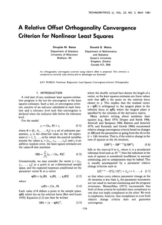
180 DOUGLAS M. BATES AND DONALD G. WATTS

Kennedy and Gentle (1980)mention a relative step
size criterion like (1.7)as well as relative changein the 1 2

sum of squares and gradient size criteria. However,
they also state that “there is no known criterion that
is absolutely satisfactory.” Chambers (1973) quotes
several other criteria, including the size of the gra-
dient and the size of the Gauss-Newton step and the
fact that the residual vector should be orthogonal to
the derivative vectors, but there is no scalesuggested
for measuring “size.”
All but the last of these are more correctly
described as termination criteria (Bard 1974) since
they merely indicate whether further iterations might
be useful according to arbitrary tolerance levels: they
are not convergence criteria since they do not neces-
sarily indicate whether a local minimum has been Y
-
attained. On the other hand, orthogonality is an abso-
lute indicator of convergence and hence it implies
that the other criteria will be satisfied.Furthermore, it
is possible to develop a meaningful tolerance level for
orthogonality based on statistical considerations.

2. DEVELOPING AND IMPLEMENTING
THE CRITERION
-1.
2.1 Relative Offset
An important consequence orthogonality is that
of
A- "2
-1.5

the residual vector has zero projection onto the tan-
I
gent plane, and so we may use the length of this 1

projection as the indicator. An appropriate scale of Figure 1. Projecting the Residual Vector Onto the
measurementcan be determined by considering the Tangent Plane
effect of this tangential component on inferences
about the parameters.
To illustrate the orthogonality convergencecriter- clared at a value rYi) close to 6, the tangential com-
ion we use a simple example in which f(x,, 0) = ponent eT will causethis disk to be slightly increased
exp(ex,) with n = 2 observations. We supposefurther in radius and offset by an amount (1 I).Therefore, we
eT
that x1 = 1 and x2 = 2. In this casethe solution locus baseour orthogonality criterion on the offset relative
is a parabola in the two-dimensional sample space to the radius of the tangent plane confidence disk. To
(Fig. l), which demonstrates the two major effectsof avoid dependenceon the confidence level we remove
nonlinear models, namely curving of the solution the factor F(p, n - p; a) and define the proportional
locus and nonuniformity of the spacing of the par- offset at f)(i)
as
ameter values.
In general, if Oci) 6 is the least squaresestimate,
= p = IleT II/(PSP’~/(~ - P))“*. (2.2)
then e = y - r@“) will have zero projection onto the The tolerance level for the criterion can now be set at,
tangent plane at n(0”‘). If it is not, the tangential say, 001, since a confidence region will not be
component eT will offset the confidence region. materially affected by the fact that the current par-
Assuming that near I@) the solution locus is rela- ameter vector f3@) lessthan one tenth of one percent
is
tively flat so it can be reasonably approximated by of the confidence region radius away from the least
the tangent plane, a (1 - M)confidenceregion consists squarespoint 6.
of those values of 0 for which When the experimental design includes replica-
tions, the residual vector contains a component that
lhm - t1@)ll* 5 PMHP, n - P; NJ/h - ~1, (2.1) is always orthogonal to the solution locus and hence
as discussed in Hamilton, Watts, and Bates (1981). to any tangent plane. This constant component,
That is, the approximate confidence region corres- which contributes the pure error sum of squaresS,,, ,
ponds to a disk on the tangent plane with radius pro- inflates the overall length of the residual vector but
portional to (pS@)/(n - p))“‘. If convergence is de- does not change I/e, /I and so the angle of the residual

A CONVERGENCE CRITERION FOR NONLINEAR LEAST SQUARES 181

vector to the tangent plane is inflated. To avoid this, (Marquardt 1963) by using the implementation
we modify (2.2) and define the relative offset as described in Golub and Pereyra (1973) in which the
first step is a QR decomposition of V. Other iterative
(IleTII/W’) methods that involve at least calculating the gradient
’ = ((s(eci)) &)/(n - p -
- v))lj2 (2.3) of S(O), such as the gradient methods described in
where v is the degrees of freedom for replications. Kennedy and Gentle (1980) would require the calcu-
This definition includes the case for no replications, lation of V so the information necessaryto calculate
since then both Srepand v will be zero and (2.3) P would be available.
reducesto (2.2).
3. DISCUSSION
2.2 Implementation It is useful to compare the termination criteria
To implement the orthogonality criterion, one recommended in the literature (e.g., Bard 1974,
must calculate IleTI( and S(Oci)) eachiteration. (The
at Chambers 1973,Draper and Smith 1966,and Meyer
replication information, v, and Sreg be determined
can and Roth 1972) and used in programs (e.g., BMD
by preprocessing the data manually or by using a P3R and BMD PAR from Dixon and Brown 1977or
computer method.) In the standard Gauss-Newton TSP. from Hall and Hall 1976)with the orthogona-
algorithm the derivative matrix lity criterion proposed here. The indicator, tolerance
level, and implementation of the criteria provide
V = dqlde (2.4) grounds for comparison.
WI
3.1 The Indicator
is evaluated at each iteration, and the parameter
vector is changed to A key feature of the offset criterion is that it pro-
vides direct information about orthogonality of a re-
@i+1)= fj(i) + k&C’+1)
(2.5) sidual vector to the solution locus, and hencerelative
where offset is an unambiguous indicator of convergence.
h(i+l) = (vfjf-1~7~ On the other hand, relative changecriteria only indi-
(2.6)
cate progressby the algorithm. Unfortunately, lack of
and k is the increment factor adjusted to ensure that progress does not imply convergenceand so prema-
S(#+ l)) < S(@) (Box 1958, Hartley 1961). To test ture termination can occur. This is evenmore likely in
whether a point Oci)is close enough to fi to declare the presence of severe nonlinearity, since then the
convergence,one could evaluate (2.3) as increment factor k may be forced to a small value and
p = (n - p - v)e’V(V’V)-‘ve 1’2 (2.7)
so relative changes in the sum of squares and the
parameters may drop below the tolerance level, re-
( (p(sv)) - k,)) i sulting in termination.
and compare this to the tolerance level. However, a As discussedby Himmelblau (1972) a small rela-
more efficient and computationally stable procedure tive change in the sum of squares does not imply
is to calculate an orthogonal-triangular decomposi- convergence, only that the sum of squaressurface
but
tion of V as is quite flat. Similarly, a small relative change in the
parametersdoesnot imply convergence, only that
but
V=QR (2.8 1 a small increment can be tolerated becauseof either
where Q is an n by p matrix with unit orthogonal intrinsic or parameter-effects nonlinearities, as dis-
columns and R is a p by p upper triangular matrix cussed by Bates and Watts (1980). Orthogonality,
(Chambers 1977). This can be done with a Gram- on the other hand, directly measures convergence,
Schmidt, Householder, or Givens method to produce and implies zero relative changes.
the increment Finally, becauserelative offset is an absolute meas-
&(i+1)= R- 1~'~. ure of convergence,it can be used to test whether any
(2.9) point is a point of convergence, regardless of the
BecauseQ has orthogonal columns that form a basis method of arriving at that point, and independently
for V, of the severity of the nonlinearity of the problem.
IleT = llQ’4~ (2.10) 3.2 The Tolerance Level
and so P is easily obtained in an intermediate step. If Becauserelative change criteria are only indirect
P exceeds the tolerance level, the iteration is indicators of convergence,the choice of appropriate
completed and the next parameter vector examined. tolerance levels is difficult. The levels are often
The criterion can be easily incorporated into pro- justified by suchconsiderationsas“There is no needto
grams basedon the Levenburg-Marquardt procedure continue iterating if the relative changein the sum of

182 DOUGLAS M. BATES AND DONALD G. WATTS

squares is less than one part in ten thousand.” Such lems the residual vector will be entirely the result of
arbitrary choices of tolerance level can result in round-off error at the minimum, and it is possible
premature termination or unnecessarycomputation that the desired degreeof orthogonality could not be
in the pursuit of unwarranted precision. Furthermore, achieved because the round-off error would effec-
in the caseof the sum of squares,a large replication tively produce a random orientation of the residual
sum of squares will cause any relative change to vector. Failure in these casesis not the fault of the
appear small, thereby increasing the probability of criterion, but results from unrealistic “zero residual”
premature termination. problems that are often usedto compare the behavior
In the caseof the parameter relative changecriter- of different convergencealgorithms. It is extremely
ion, its form suggeststhat it is based on numerical unlikely to encounter such data in practice.
considerations, since computation halts when the re- There can also be circumstances in which ortho-
lative accuracy of each parameter estimate appears gonality cannot be achieved because the solution
adequate.Statistical considerations suggest,however, locus is finite in extent and the data vector lies “off the
that a more appropriate scalewould be basedon the edge.” These cases are often discovered when one
inherent variability of the estimates. In our criterion parameter is forced out to infinity or negative infinity
since convergenceis measuredby offset relative to the or the derivative matrix becomes singular. An
residual variation, the tolerance level is easily as- example of this is example 5 from Meyer and Roth
signed a sensible value on a meaningful scale thus (1972)where the minimum actually occurs with el at
avoiding both premature termination and unproduc- infinity. In such circumstances the data analyst
tive computation, should realize that the model does not fit well to the
data and that alternate models should be employed.
3.3 Implementation The relative offset criterion provides such informa-
Various forms of the relative change criteria have tion, but a relative change criterion based on lack of
been implemented. For example, the BMDP series progress would not.
programs use only a sum of squares termination
criterion with a tolerance level of lo- 5 subject to the 3.4 Examples
requirement that the criterion be satisfied on five We were motivated to develop the orthogonality
successive iterations. We suspect that while this convergence criterion by the discovery that for
would ensure convergencefor most problems, it ob- several examplesin the literature the residual vector
viously involves arbitrary, and probably conservative, was not at all close to being orthogonal at the
choices of the tolerance level and number of repeti- reported parameter estimates. This usually occurred
tions. (Even so, there is no guaranteeof convergence when the data were simulated with small residual
since the criterion may be fooled by parameter-effects variance and the estimateswere rounded in reporting.
nonlinearity.) Example 8 of Meyer and Roth (1972)has a relative
The relative parameter increment criterion appears offset of 208 percent at the reported parameter values
in different forms (Bard 1974,Draper and Smith 1966, 0 = (.0056, 6181.4, 345.2)‘, which corresponds to an
Marquardt 1963, and Kennedy and Gentle 1980). angle of 12”. In addition, the reported parameter
One modification to avoid small parameter values values produce a sum of squaresof 2021.9,instead of
inflates the denominator of (1.7) by a small positive the 88.0 quoted in the paper. Even when the estimates
quantity r so as to avoid division by zero. This ver- are recalculated and rounded to six significant digits
sion is clearly sensitiveto scaling or transformation of to yield the parameter vector 8 = (.00560964,6181.35,
the parameters and could result in different termina- 345.224)‘, there was still an offset of 6.9 percent
tion with different scaling or parameterization, although the sum of squares did in fact go down to
especially since the choice of r is quite arbitrary. 88.04. When the estimates were reported to a lower
Although the two relative-change criteria have accuracy by rounding them to five significant digits,
been widely used and have probably been quite the offset increased to 27 percent and the sum of
successful,they can be easily replaced by one simple squaresincreasedto 89.45.For this example there is a
relative-offset convergencecriterion that does not re- very high correlation between the parameter esti-
quire ad hoc modifications to avoid pathological mates,and the effect of rounding theseestimatesis to
complications and that provides a direct unequivocal produce values that would not even fall in the proper
indication of convergence. 95 percentjoint confidenceregion. Note that the rela-
There is, however, one type of problem for which a tive offset can be measuredat the rounded parameter
relative offset criterion or any other criterion based values without any information on the way that those
on orthogonality is inappropriate: the least squares values were obtained, which is not the case for
problem using simulated data for which the residual relative-changecriteria.
sum of squarescan be reduced to zero. In theseprob- A similar situation occurs with the example in Box

A CONVERGENCE CRITERION FOR NONLINEAR LEAST SQUARES 183

and Hunter (1963) which uses all 13 data points. of Canada, the University of Alberta General
There is a high replications sum of squares(the F for ResearchFund, and the Queen’sUniversity Advisory
lack of fit is .056) that inflates the length of the resi- ResearchCouncil.
dual vector, but not the projection, so the relative
[Received June 1979. Revised December 1980.1
offset using (2.3) at the reported parameter values of
8 = (3.57, 12.77, 0.63) is 8.2 percent. Further itera-
tions indicate that five significant digits are required
to produce an offset less than .l percent for the par-
ameter vector 8 = (3.5691, 12.800,.62950)‘.We note
REFERENCES
that the second parameter does not round down to
the reported value if four significant digits are used. BARD, Y. (1974) “Nonlinear Parameter Estimation,” New York:
Academic Press.
4. SUMMARY BATES, D. M., and WATTS, D. G. (1980), “Relative Curvature
Measures of Nonlinearity” (with discussion), J. Roy. Statist. Sot.,
A relative offset convergencecriterion for nonlinear Ser. B, 42, l-25.
least squareshas been proposed, basedon the size of BOX, G. E. P. (1958), “Use of Statistical Methods in the Elucidation
the projection of the residual vector in the tangent of Physical Mechanisms,” Bull. International Statistical Institute,
plane relative to the radius of the confidence region 36, 215-225.
BOX, G. E. P., and HUNTER, W. G. (1963) “Sequential Design of
disk on that tangent plane. Becausethe criterion is Experiments for Nonlinear Models,” in Proc. IBM Scientijc
based on orthogonality, it embodies the following Computing Symposium Statistics, White Plains, N.Y.: IBM.
advantages: BOX, G. E. P., and LUCAS, H. L. (1959). “Design of Experiments
in Nonlinear Situations,” Biometrika, 46, 77?-X1.
I It provides an absolute measure of conver- CHAMBERS, J. R. (1973) “Fitting Nonlinear Models: Numerical
gence. On the other hand, relative change Techniques,” Biometrika, 60, 1-13.
values are merely termination criteria, and - (1977) Computational Methods for Data Analysis, New
compliance of relative changevalues to toler- York: John Wiley.
DIXON, W. J., and BROWN, M. B. (eds.) (1977), BMDP-77
ance levels does not imply convergence. Biomedical Computer Programs, P-Series, Los Angeles: Univer-
II It is independent of any scaling of the data, of sity of California Press.
linear or nonlinear transformations of the par- DRAPER, N. R., and SMITH, H. (1966) Applied Regression
ameters, and of the method used to arrive at Analysis, New York: John Wiley.
the test point. GOLUB, G. H., and PEREYRA, V. (1973) “The Differentiation of
Pseudo-Inverses and Nonlinear Least Squares Problems Whose
III It is applicable to Gauss-Newton and gradient Variables Separate,” J. SIAM, 10,413-432.
methods. HALL, ROBERT, E., and HALL, BRONWYN, H. (1976) Time
IV It is independent of conditioning of the prob- Series Processor, Cambridge: Harvard Institute of Economic
lem and of parameter-effectsnonlinearities. Research, Harvard University.
V It provides a meaningful scaleof measurement HAMILTON, D. C., WATTS, D. G., and BATES, D. M. (1981)
“Accounting for Intrinsic Nonlinearity in Nonlinear Regression
for orthogonality based on statistical con- Parameter Inference Regions,” unpublished paper.
siderations. This permits one to specify appro- HARTLEY, H. 0. (1961) “The Modified Gauss-Newton Method
priate tolerance levels to avoid both for Fitting of Nonlinear Regression Functions by Least Squares,”
premature termination and unproductive Technometrics, 3, 269.
computation. On the other hand, relative HIMMELBLAU, D. M. (1972) “A Uniform Evaluation of Uncon-
strained Optimization Techniques,” in Numerical Methods for
change criteria involve arbitrary decisions Nonlinear Optimization, ed. F. A. Lootsma, London: Academic
concerning tolerance levels. Press.
VI It provides a meaningful link betweenstatisti- JENNRICH, R. I., and SAMPSON, P. F. (1968) “Application of
cal measuresof precision (i.e., the confidence Stepwise Regression to Nonlinear Estimation,” Technometrics,
region radius) and numerical measures of 10, 63-72.
KENNEDY, W. J., Jr., and GENTLE, J. E. (1980) Statistical
precision (i.e., the number of significant digits) Computing, New York: Marcel Dekker.
and hencedictates the necessaryand sufficient MARQUARDT, D. W. (1963) “An Algorithm for Least Squares
number of digits to be used in reporting each Estimation of Nonlinear Parameters,” J. SIAM, 11, 431-441.
parameter value. MEYER, R. R., and ROTH, P. M. (1972) “Modified Damped
Least Squares-An Algorithm for Nonlinear Estimation,” J.
5. ACKNOWLEDGMENTS Inst. Math. Applies., 9, 218-253.
RALSTON, M. L., and JENNRICH, R. I. (1978) “Dud, a
This research was supported by grants from the Derivative-Free Algorithm for Nonlinear Least Squares,” Tech-
Natural Sciencesand Engineering ResearchCouncil nometrics, 20, 7-14.


V2302179

Recommended

Recommended

More Related Content

What's hot

What's hot (9)

Similar to V2302179

Similar to V2302179 (20)

V2302179