![Bode plot : visualization of transfer function
Modal analysis : transfers
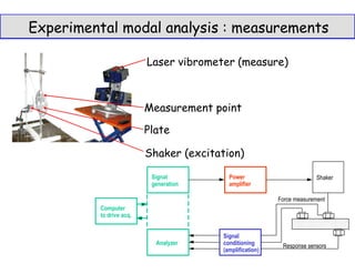
In
U
Out
Y
System H
{Y(w)}=[H(w)]{U(w)}
ONE input
ONE output
MANY resonances
Transfers estimated
from time response](data:image/gif;base64,R0lGODlhAQABAIAAAAAAAP///yH5BAEAAAAALAAAAAABAAEAAAIBRAA7)
Recommended
More Related Content
Similar to CM2_Mode.pdf
Similar to CM2_Mode.pdf (20)
Recently uploaded
Recently uploaded (20)
CM2_Mode.pdf
- 1. Shaker (excitation) Plate Laser vibrometer (measure) Measurement point Experimental modal analysis : measurements Computer to drive acq. Signal generation Power amplifier Shaker Force measurement Response sensors Signal conditioning (amplification) Analyzer
- 2. Bode plot : visualization of transfer function Modal analysis : transfers In U Out Y System H {Y(w)}=[H(w)]{U(w)} ONE input ONE output MANY resonances Transfers estimated from time response
- 3. 1 input, 1 output, many resonances Spectral decomposition MDOF (multiple resonances) SISO Tj is 1x1 Note : series truncated in practice constant approximation of high frequencies (D term in states space models) MDOF multiple degree of freedom SISO single input single output
- 4. MDOF MIMO system • Poles depend on the system (not the input/output) • The shape is associated with the input/output locations The shapes The poles
- 5. Lagrange equations / virtual power principle Kinematics • Displacement • Strain Statics/thermodynamics • Load/Stress • Power : Constitutive law (behavior) Equations of motion Will be detailed in CM3
- 6. Kinetic energy (mass matrix) Strain energy (stiffness matrix) Work of external load (here constant) Lagrangian Lagrange equations of motion (generally valid for NL non-linear systems) Leads to Lagrange equations (in advance of CM3 needed TD2)
- 7. Modes : harmonic solution with no force complex mode (general definition) Eigenvalue problem Linear time invariant https://www.youtube.com/watch?v=zstmGnaaaCI
- 8. • Real mode : no damping / elastic / conservative • M>0 & K0 f real • There are distinct modes for DOF • Full solver : scipy.linalg.eig (LAPACK Linear Algebra) • Partial solvers exist, a few keywords – scipy.sparse.linalg.eigs (Matlab eigs) : Arnoldi – FEM Solvers : Lanczos (Krylov+conjugate gradient), AMLS Normal modes of elastic structure 34
- 9. Normal modes of elastic structure • Orthogonality • Scaling conditions • Unit mass • Unit amplitude 35
- 10. Kinematics / model reduction • Displacement u(x,t) = shapes (x) x DOF (t) {q}N= qR Nx NR T Ph.D. Corine Florens 2010 In Out System States Quasi-static response @ 10Hz = • Modes : high energy, load independent (no blister shape) • Static response (influence of input=blister), important away from resonance 36 Variable separation
- 11. Modal (principal) coordinates • Coordinate change (physical , generalized ): • Inject in equations of motion • Over determined ( ) : compute “virtual work” • For modes Reduced mass Reduced stiffness Reduced load, reduced observation 37
- 12. Observation • {y} outputs are linearly related to DOFs {q} using an observation equation • Simple case : extraction • More general : intermediate points, reactions, strains, stresses, … Illustrations TD1 (q3f, q6f) TD3 (q3a), TD5, … 38
- 13. Command • Loads decomposed as spatially unit loads and inputs {F(t)} = [b] {u(t)} Abaqus : *CLOAD + *AMPLITUDE, … NASTRAN : FORCE-MOMENT + RLOAD ANSYS, CODE Aster, … Illustrations TD1, 3, 5, … 39
- 14. Rayleigh damping – Physical domain – Modal domain = 𝒋 𝒋 Modal damping derived from test 40 Modal damping O. Vo Van, E. Balmes, et X. Lorang, « Damping characterization of a high speed train catenary », IAVSD, Graz, 2015, http://sam.ensam.eu/handle/10985/10918. Reality Mass Stiffness can be > 100% Physical domain 𝒋 𝒋
- 15. • Physical • Modal coordinate • Modal equations (modal damping) 𝒋 𝒋 • Reduced matrices = diagonal Modal observability/commandability • Spectral equations (inverse of diagonal matrix) 41 Physical / modal & spectral decomposition Exam
- 17. Mots clefs du CM • Définition mathématique des modes pour un modèle discret, orthogonalité, normalisation (s3.2) • Expression de la fonction de transfert en base modale, masse et raideur modale, expression des contributions sous forme de série (formule (3.29)) • Observabilité f(3.4) et commandabilité f(3.3) modale f(3.35) • Amortissement modal, amortissement de Rayleigh (s3.4) • Troncature 43