SlideShare a Scribd company logo
1 of 53
Download to read offline
Detecting Auctioneer Corruption: Evidence from
Russian Procurement Auctions∗
Pasha Andreyanov Alec Davidson Vasily Korovkin†
UCLA UCLA UCLA
July 2018
Abstract
This paper develops a novel method for detecting auctioneer corruption in first-price sealed-bid
auctions. We study the leakage of bid information by the auctioneer to a preferred bidder. We
construct a formal test for the presence of bid-leakage corruption and apply it to a novel data
set of 4.3 million procurement auctions in Russia that occurred between 2011 and 2016. With
bid leakage, the preferred bidder gathers information on other bids and waits until the end of the
auction to place a bid. Such behavior creates an abnormal correlation between winning and being
(chronologically) the last bidder. Informed by this fact, we build several measures of corruption.
We document that more than 10% of the auctions were affected by bid leakage. Our results imply
that the value of the contracts assigned through these auctions was $1.2 billion over the six-year
study period. We build a model of bidding behavior to show that corruption exerts two effects on
the expected prices of the contracts. The direct effect inflates the price of the contract. The indirect
effect reduces the expected price, since honest bidders are trying to undercut corrupt bidders. We
find both effects in the data, with the direct effect being more pronounced.
JEL: H57, D44, D73, L40.
Keywords: Corruption, Procurement Auctions, Detection
∗
We are grateful to John Asker, Leonardo Bursztyn, Lorenzo Casaburi, Ernesto Dal Bo, Christian Dippel, Geor-
gy Egorov, Siddharth George, Stefano Fiorin, Gaston Illanes, Seema Jayachandran, Kei Kawai, Lidia Kosenkova,
Alexey Makarin, Imil Nurutdinov, Ricardo Perez-Truglia, Nicola Persico, Robert Porter, Nico Voigtländer, Romain
Wacziarg, Noam Yuchtman, and the participants of the Brown Bag at the Anderson School of Management, DE-
VPEC2016, GEM-BPP workshop, RSSIA2016, NEUDC2016, Northwestern IO lunch, IIOC2017, MWIEDC2017,
and TADC2017 for helpful comments and suggestions. Vasily Korovkin thanks the UCLA Anderson Center for Glob-
al Management for financial support.
†
Corresponding author. E-mail: vaskorovkin@gmail.com.
1 Introduction
An extensive empirical and theoretical literature is dedicated to detecting collusion in auctions.1
In
contrast, the literature on detecting corruption in auctions—unsavory agreements between bidders
and an auctioneer—is virtually nonexistent. Extensive evidence shows that in the context of public
procurement—particularly in emerging economies—corruption can exert a strong effect on the
inefficient use of public funds (Kenny, 2007; Olken and Pande, 2012).2
Corruption in procurement
can take many forms. So far there has been no systematic evidence on the exact channel by
which corruption leads to inefficient allocation of public funds in procurement. Since procurement
auctions are a common tool by which public projects are assigned to firms, they are also a natural
candidate for such channel.
This paper examines an endemic type of corruption in procurement—“bid leakage” in first-
price sealed-bid auctions. Under bid leakage, an auctioneer forms an agreement with one of the
bidders to reveal information on all other bids. The preferred bidder can then decide how to place
her bid. In the public procurement setting, the auctioneer is a government official who represents
a public body, and the bidders are representatives of firms bidding for the contract. We start by
developing a method to detect and measure the extent of bid leakage. At the core of our approach
is the information on the timing of bids. We apply our method to the universe of first-price sealed-
bid procurement auctions held by Russian public bodies from 2011 to 2016. We collected this data
set from Russia’s centralized official procurement website.3
The data cover small procurement
contracts all over the country, including detailed records of the bids by each contractor, together
with the time at which each bid was placed. The time stamps are a unique feature of the data that
allows us to detect and measure corruption.4
Our first approach exploits the fact that the preferred bidder wants to collect all information on
the other participants’ bids and thus bids last. We calculate the probability of winning conditional
1
See Marshall and Marx (2012), Whinston (2008), and Porter (2005) for cases of collusion and methods of detec-
tion.
2
The 2013 OECD “Corruption in Procurement” brochure (http://www.oecd.org/gov/ethics/Corruption-in-Public-
Procurement-Brochure.pdf) states that in OECD countries public procurement accounts for 12% of GDP and 29% of
government expenditure, totaling 4.2 trillion euros. In Russia (http://www.interfax.ru/business/499881), it was 25%
of the 2016 GDP. As the OECD Foreign Bribery Report (http://www.oecd.org/corruption/oecd-foreign-bribery-report-
9789264226616-en.htm) shows, more than half of foreign bribery cases concerned obtaining a government contract.
Furthermore, Transparency International claims that project costs can, as a result, increase as much as 50%.
3
http://zakupki.gov.ru.
4
To our knowledge, time-stamp data are unavailable for the existing sealed-bid auction data sets (as opposed to
open auctions). In addition, our new auction data set is one of the largest, with 4.3 million auctions and more than 10
million bids.
1
on being the last to bid. In the absence of corruption, bidding and timing decisions are independent,
and this probability would be equal to the inverse of the number of participants (that is, three
bidders should each have a 1 in 3 chance of winning). In the data, for auctions with three bidders,
the probability of winning conditional on bidding last is 0.397, while the probability of winning
conditional on not bidding last is 0.301. Comparing the two numbers, we test for the presence
of corruption. In addition, the difference between the probabilities allows us to infer the share of
corrupt auctions, that is, to measure corruption.
Our baseline approach is intuitive, but it uses only the information on the probability of winning
for the last bidder and for all other bidders. A complementary approach is to use the distribution
of timing for the winners and the other bidders to measure the abnormal mass of winning bids
placed near the deadline. The share of corrupt auctions can then be estimated from a normalized
difference of the cumulative distribution functions of timing for the winner and the runner-up. This
approach yields similar quantitative results.
This measure of corruption shows that 10.8% of auctions are affected by bid leakage. The
absolute number of contracts affected is 25,000—a number that balloons to over 380,000 if we
scale up the estimate to the six-year study period. The value of affected contracts was as high as
$1.2 billion.5
Once we measure corruption for the whole sample, we can repeat the exercise for a subsample
of frequent auctioneers and bidders. That is, we can calculate the difference in conditional proba-
bilities separately for each auctioneer and each bidder. This helps to determine which auctioneers
and bidders are more corrupt. In this sense, we follow the literature that detects collusive groups
of bidders (Kawai and Nakabayashi, 2014; Porter and Zona, 1999).
In the second part of our analysis, we examine the consequences of corruption for the expected
prices that public bodies paid for the contracts. We build a model of bidding behavior. The model
predicts that while a direct effect of corruption increases the expected price of the contract, corrup-
tion can also affect prices indirectly by changing the behavior of honest bidders. Intuitively, honest
bidders behave more aggressively by reducing their bids. As a result, this equilibrium response can
lower average prices of procurement contracts as opposed to inflating them, as would be natural
with corruption. Nevertheless, the net effect on prices for standard distributions of costs is still
5
As a benchmark, we can compare these numbers to a large-scale estimate of collusion from Kawai and
Nakabayashi (2014). To our knowledge, they have provided the only estimate of collusion measured across a na-
tion, even though they cover only one industry. Kawai and Nakabayashi (2014) show that collusive bidders were
awarded 7,600 construction projects worth $8.6 billion in Japan, equal to 19% of national government construction
projects. Their scaled-up estimates suggest that 0.85% of the GDP of Japan was affected.
2
positive. That is, the direct effect of corruption is larger in magnitude than the indirect effect.
We test the predictions of the model starting with a reduced-form estimation. We regress the
final prices of the contracts and the bids on the measures of corruption of the auctioneers and the
bidders, as well as the interaction between auctioneer and bidder corruption. For bidders with
low measure of corruption, higher auctioneer corruption is associated with lower bids, while for
more corrupt bidders, auctioneer corruption increases the bids. If we interpret our estimates as
causal, reducing the share of corrupt auctions from mean value of 0.1 to zero reduces prices by
3%.6
This estimate hides important heterogeneity. If we concentrate on the subsample of frequent
auctioneers and bidders, corruption has a nonlinear effect on prices. For this subsample, there is a
nonzero optimal level of corruption.
In the third part of our analysis, we estimate our model structurally to confirm that bidding be-
havior changes in line with the model. We restrict our analysis to the bidding behavior of bidders
with low estimated share of corrupt auctions—“honest bidders.” We compare how honest bidders
bid when they participate in the auctions with corrupt and with noncorrupt auctioneers. We follow
the existing literature on the estimation of the valuations (costs) from the bidding data using the
first-order conditions in Guerre, Perrigne, and Vuong (2000), and extend their approach to incor-
porate bid leakage and to estimate bid functions and the underlying distribution of costs. This
approach allows us to estimate bid functions of honest bidders separately for each auctioneer. For
more corrupt auctioneers, bid functions of the honest bidders shift downward. That is, for the same
value of the underlying costs, they bid more aggressively, which is in line with our reduced-form
results.
Relative to existing literature, we make several contributions. First, we detect corruption (an
agreement between an auctioneer and one of the bidders) as opposed to collusion (an agreement
between two or more bidders) noted in previous literature.7
Our paper is the first to build a method
for corruption detection in first-price sealed-bid auctions and one of the first papers to empirically
study corruption in auctions.8
At the same time, we draw insights on the bid-leakage corruption
6
If we compare these effects with the existing studies of corruption in similar frameworks, our results are some-
what smaller in magnitude. Di Tella and Schargrodsky (2003) reported that a crackdown on corruption in Argentinean
hospitals reduced procurement prices by 10%. Bandiera, Prat, and Valletti (2009) showed that active waste in Italian
public procurement increased prices by 11%. Other papers: Ferraz and Finan (2011); Olken (2006, 2007); Reinikka
and Svensson (2005) in various settings show estimates of loss from 9% to 24%. Although these papers study pro-
curement and corruption in distribution of pubic funds, they do not study the bidding data in procurement auctions.
7
See Porter (2005), and Asker (2010a) for a review of the literature on collusion in auctions, as well as Hendricks
and Porter (1988); Porter and Zona (1993); Baldwin, Marshall, and Richard (1997); Porter and Zona (1999); Pesendor-
fer (2000); Bajari and Ye (2003); Ishii (2009); Asker (2010b); Athey, Levin, and Seira (2011); Conley and Decarolis
(2011); Haile, Hendricks, Porter, and Onuma (2012); Kawai and Nakabayashi (2014); Schurter (2016).
8
With a notable exception of Cai, Henderson, and Zhang (2013), who examine corruption in auction design in land
3
in auctions from a vast theoretical literature.9
Our model of strategic behavior of honest bidders
extends Arozamena and Weinschelbaum (2009) to allow the level of corruption to be uncertain and
vary across auctioneers. None of the existing theoretical papers provide any empirical evidence on
this type of corruption, nor on offsetting effects of corruption on prices in auctions.10
We also contribute to the literature on inefficiencies in procurement.11
This literature perceives
the mechanism of allocating a contract as a black box, while we stress how corruption changes the
outcomes of auctions and subsequently distorts the contract prices. Moreover, little is known on
how equilibrium response of honest agents can change the implications of corruption. Although
percentage estimates of loss are of a similar order of magnitude to those in the existing literature,
we point out that corruption can have severe implications for the behavior of the noncorrupt bidders
through the indirect effect.
From the policy side, our paper contributes to the literature on electronic procurement (Elbah-
nasawy, 2014; Lewis-Faupel, Neggers, Olken, and Pande, 2014; Best, Hjort, and Szakonyi, 2017)
and e-governance in general (Banerjee, Duflo, Imbert, Mathew, and Pande, 2014; Muralidharan,
Niehaus, and Sukhtankar, 2014). One policy lesson from our paper is that recording the timing
of bids is extremely helpful for detecting various types of illegal behavior and for measuring their
magnitude.
The rest of our paper is organized as follows. Section 2 describes the institutional background
and the details of the procurement procedure that we analyze. Section 3 describes the data and
illustrates the ideas behind our methods using simple graphical analysis. Section 4 sets up tests and
measures for corruption and shows the results of the estimation. Section 5 presents a stylized model
of bidding behavior under bid leakage and examines the expected prices of the contracts with and
without corruption. Section 6 explores how corruption varies across auctioneers and bidders and
provides reduced-form estimates of the effect on prices in a reduced-form way. Section 7 presents
markets in China.
9
See for instance, Compte, Lambert-Mogiliansky, and Verdier (2005); Menezes and Monteiro (2006); Lengwiler
and Wolfstetter (2006); Burguet and Perry (2007); Arozamena and Weinschelbaum (2009); Lengwiler and Wolfstetter
(2010).
10
We are also the first to exploit the timing as a strategic variable in sealed-bid auctions as opposed to open auctions
(such as eBay). We show that timing can matter even in sealed-bid auctions, without any considerations that are usually
relevant to open auctions (see, for example, Bajari and Hortacsu, 2003; Ockenfels and Roth, 2002, 2006; Hendricks,
Onur, and Wiseman, 2012; Hopenhayn and Saeedi, 2015).
11
Existing papers attribute the inflation in contract prices to different inefficiencies, such as political connections
(Schoenherr, 2014; Callen and Long, 2015; Baltrunaite, 2016; Coviello and Gagliarducci, 2016; Guerakar and Mey-
ersson, 2016), red tape (Bandiera, Prat, and Valletti, 2009; Lewis-Faupel, Neggers, Olken, and Pande, 2014; Best,
Hjort, and Szakonyi, 2017), or corruption (Shleifer and Vishny, 1993; Di Tella and Schargrodsky, 2003; Ferraz and
Finan, 2008; Mironov and Zhuravskaya, 2014).
4
the structural estimation of bid functions of different groups of auctioneers. Section 8 concludes.
2 Institutional Background
In Russia public procurement accounted for 25% of 2016 GDP.12
Most contracts are allocated
through auctions. The three most widely used auction types are requests for quotation, open auc-
tion, and open tender.13
We focus on requests for quotations, or, as we call them interchangeably throughout the paper,
first-price sealed-bid auctions, which is the format used for small contracts. The reserve price of
such a contract cannot exceed 500,000 rubles (≈$8,800),14
and no more than 100 million rubles
(≈1.8 million) per year can be assigned this way.15
Typical examples of these contracts are pur-
chases of office supplies for a municipality, books for a public school, or medical supplies for a
public hospital. Small repairs, street cleaning, and other types of services can be purchased through
this format as well. Requests for quotations require less paperwork for the public body, but they
are also less transparent for the controlling agencies to oversee.
A request for quotations proceeds as follows: a public body posts an announcement of the
auction at the designated website. The format of the public notice is standardized; the notice
contains exhaustive information about the contract, including the deadline to submit a bid and
the requirements to qualify as a bidder. For larger contracts, the public body has to upload an
announcement to the website not less than seven business days before the deadline of the auction.
When the auction is live, any eligible firm can submit an application, which has to include a
contract price (we call it a “bid”), together with the documentation that confirms the eligibility of
the firm. The majority of applications are submitted in sealed envelopes that are usually hand-
delivered by a representative of the applicant. In the first part of the study period applications
could have been submitted via email with an electronic signature, however recently the number of
such applications declined. We discuss the reasons for that and the importance of the difference
between paper and electronic submissions later in this section.
After the auction has ended, the applications are opened by the auctioneer. Applications can be
rejected if the bidders do not meet the posted requirements. If there was only one bidder and the
12
In absolute numbers, that is ≈$530 billion. Click here to update the exchange rate. The information is from the
Ministry of Economic Development for 2016 (in Russian): http://www.interfax.ru/business/499881.
13
A request for quotation is a first-price sealed-bid reverse auction. An open auction is an online version of a reverse
English auction—the participants observe each other’s behavior and compete online. The third type, the open tender,
resembles a first-price sealed-bid reverse auction, but it takes into account the quality that a bidder can provide. In
other words, it is a scoring auction.
14
Click here to update the exchange rate.
15
Click here to update the exchange rate.
5
bidder is eligible, the contract is signed with this bidder. The winner is determined by the lowest
bid. If the bids have equal price offers, the earlier bid wins. The public body posts the results of
the auctions on the public website.16
We illustrate the timeline of a typical auction in the graph
below, using actual data.
• • • •
August 1
Public notice
is posted:
Reserve price is
$1,430
August 11
Sealed Bid 1:
$999
August 12
Sealed Bid 2:
$1,085
August 13
Deadline:
Bid 1 Wins
2.1 Bid-Leakage Corruption
Corruption in procurement happens in several ways. We concentrate on one generic type of cor-
ruption that sealed-bid auctions are especially prone to—bid-leakage corruption. Bid leakage is an
agreement between an auctioneer and one of the bidders in an auction. The auctioneer shares with
one of the bidders—whom we call the preferred or corrupt bidder—details of the bids of other
participants. Once the corrupt bidder is confident that all other bids have been placed, and if she
finds it profitable to bid, she places her bid. If she is not overly concerned with being caught by a
higher-level authority, she can undercut the current best bid by as little as possible.17
To illustrate our detection approach, we start with several examples from a major online forum
that discusses issues of public procurement in Russia.18
In the first example, Firm A participated in
five auctions organized by the same public body. Each auction had four bidders and a reserve price
in rubles equal to $6,000. In each of the five auctions, Firm A came in second, by margins of $0.50
to $12. The same company won all five auctions. In another case, Firm B faced a similar situation,
and the winner was also always the last firm to bid. In one extreme case, Firm C complained that
it was always second in 60 auctions in a row. It always lost by less than 0.5% of the reserve price,
always by around 0.5% of its own bid, and always to the same firm, which placed its bids last. This
behavior suggests that the winner knew the bid of the complaining firm and waited until the end
of the auction to place its sealed bid.19
These three examples highlight something we will focus
on—late bidding by the winner.
16
The bidders or their representatives have a right to be present for the opening procedure, can request that any
information from the bidding envelopes be disclosed, and can make a video recording of the procedure.
17
Appendix A discusses a method for detecting bid-leakage based solely on the differences in bids.
18
http://forum.gov-zakupki.ru/.
19
Here are the links to these and other cases from this forum (in Russian): (1), (2), and (3).
6
Bid leakage is not unique to Russia. Examples abound from many other countries, both devel-
oped and developing. For instance, the government of Singapore banned Siemens for five years
from participating in any public procurement auctions after the company bribed an official to learn
the bids of their competitors. Similar abuses occurred in Berlin over the contract for building a
new airport (Lengwiler and Wolfstetter, 2006). In several Italian auctions, corrupt bureaucrats
used a laparoscope to get inside the sealed envelopes without damaging them.20
Ingraham (2005)
documented cases of corruption in school construction auctions in New York City.
2.2 Bidder Response
To what extent do honest bidders react to bid-leakage corruption? We draw our motivation from
the same online forum. The bidders discuss two forms of their reaction to bid-leakage corruption:
response in timing and response in bids.21
These bidders argue that response in timing would not
be very effective: the preferred bidder will still submit an envelope at the last moment.22
One of the
participants suggested that reducing bids could be effective, since the preferred bidders would find
it not profitable to win the contract.23
Thus, anecdotal evidence suggests that honest bidders should
engage in more aggressive bidding. We model the bidding response in Section 5 and examine it
empirically in our estimation in Sections 6 and 7.
If bids were submitted via email with an electronic signature, the timing response could be
more effective for honest bidders. In the first part of the study period (2011 to 2013), as many
as 37% of the applications were submitted electronically. Since we do not know whether those
electronic submissions were encrypted or not, we have to be careful with this subsample due to
potential timing response. The electronic submission of applications was effectively eliminated
in the second part of the study period (2014 to 2016)—only 1.6% after 2013 were submitted
electronically. We apply our methods to the latter period, but we also directly test for strategic
timing response.
20
The link that discusses the case (in Italian): http://www.ilfattoquotidiano.it/2016/06/27/corruzione-appalti-
truccati-10-arresti-dirigente-comune-usava-laparoscopio-per-sapere-in-anticipo-contenuto-buste/2862756/.
21
Examples here https://web.archive.org/web/20180123052630/http://forum.gov-zakupki.ru/topic40009.html and
here: https://web.archive.org/web/20180123055013/http://forum.gov-zakupki.ru/topic40009-40.html.
22
Potentially, she can submit the envelope even after the deadline: https://web.archive.org/web/20180123053745/http://forum.gov-
zakupki.ru/topic40009-10.html
23
https://web.archive.org/save/http://forum.gov-zakupki.ru/topic40009-30.html#p4720
7
2.3 Change of Regulations
The Russian government has been declaring a fight against corruption for many years.24
Part of
this struggle centers on transparency in public procurement.
One of the government’s measures to promote transparency and reduce corruption in procure-
ment was a new piece of federal regulation—Federal law #44. The law mandates that the public be
given access to all of the procurement information. It also standardizes the format for all procure-
ment documents, which must be published online, and specifies personal responsibility of public
bodies in case of violations, among other steps.25
Another important measure is an introduction of
online standardized bidding system that needs to be used for any type of procurement procedure.
In practice, the actual implementation of the platform was postponed, first to 2017, and then to
2018. As a result, submitting bids in any electronic form became illegal, and up to discretion of a
public body.26
In the first part of the paper we study the period after the introduction of FZ#44, since it
allows us to not worry about the strategic response in timing. Once we measure corruption for this
subsample we use our auctioneer-level estimates to test the model for the whole sample, including
the period of 2011 to 2013.
3 Data
We downloaded a digital archive of all procurement auctions from January 2011 through the end
of 2016.27
The archive contains announcements and protocols, all in .xml format. A typical an-
nouncement includes information on the terms of the contract, the reserve price, the auction dead-
line, and the deadline by which the work specified in the contract should be delivered. Protocols
include the bid for each application, the time-stamp, and also whether the bid was accepted or
rejected.
We matched the announcements to the protocols and extracted all of the necessary information
by parsing each of the .xml files to get the information in each tag. The resulting data set has
more than 4.3 million requests for quotations, and more than 10 million bids. We dropped auctions
24
Putin declared the fight against corruption in 2000 (http:/kremlin.ru/events/president/transcripts/24138) and kept
declaring it every year since then. The 2015 quote: https://web.archive.org/save/https://www.1tv.ru/news/2015-03-
04/20595-v_putin_borba_s_korruptsiey_vo_vlastnyh_strukturah_budet_vestis_posledovatelno_i_zhestko.
25
This link (in Russian): http://www.garant.ru/actual/contracts/472245/ describes other measures, including mi-
nor changes in the assignment mechanisms, introduction of long-run planning, anti-dumping measures, amended for
voiding or changing the contract, and introduction of organized audits of the results.
26
Discussion between the participants: https://web.archive.org/web/20180123061015/http://forum.gov-
zakupki.ru/topic13530-410.html.
27
Available in FTP or HTML formats from the official website http://zakupki.gov.ru.
8
with any quote being rejected and auctions with fewer than three quotes, leaving us with 841,552
request for quotations.28
Table 1 of Appendix C shows summary statistics for the whole period covered and for the new
law, FZ#44 (2014–2016). The reserve price in requests for quotations is a maximum price that
the winning bid cannot exceed in order for the auction to be considered valid. For requests for
quotation this reserve price has lower than 500,000 rubles, or $8,700, as of the current exchange
rate.29
In our sample, the mean reserve price is 213,507 rubles ($3,718).30
The mean winning
bid is 157,850 rubles ($2,749),31
while the mean ratio of the winning bid to the reserve price is
73.3%.32
Figure 1 shows that the number of bids placed in the last hours before the deadline is large
for all bidders; however, the winner tends to bid later asymmetrically more than the other bidders.
Most of the extra density for the winner comes from the last minutes of the auction. The densities
for the second, third, and fourth bidders are practically indistinguishable from each other. This
is an exact pattern that we expect to see in the presence of bid leakage: even with a substantial
share of bids placed in the last day, the winners tend to bid asymmetrically closer to the deadline,
with a gap more pronounced in the last hours of the auction. In the next section we quantify this
asymmetry between the winners and all other bidders, in order to detect and measure corruption.
28
The auctions without quotes do not provide any insights for our analysis. Neither do the rejected bids. We do not
use the auctions with one or two bidders in our main analysis since we cannot employ our methods without observing
a third bid.
29
Click here to update the exchange rate.
30
Click here to update the exchange rate.
31
Click here to update the exchange rate.
32
For more details on the reserve price distribution and the distribution of the winning bid one can resort to Appendix
C. Panel A of Figure C1 shows that the distribution of reserve prices has almost a full support from 0 to 500,000 rubles.
The empirical density of the reserve price is monotonically decreasing apart from the spikes at round numbers and
especially on the maximum level of 500,000 rubles, and except for the neighborhood of 0. Panel B of Figure C1 shows
that the winning bids have a similar distribution, but without a spike at 500,000 rubles.
9
Figure 1: Hours to the Deadline for the Top Four Bidders
0 5 10 15 20
0.000.020.040.060.08
Last 24 hours; N = 112,525
Density
Densities of Timing, Kernel Estimates
By Bidder Rank
Winners
Runners−Up
3rd−Best
4th−Best
Notes: Kernel density estimates for the timing of bids. Distance in hours to the deadline over the last twenty four hours. The densities are drawn
separately for the winning bids, the runner-up bids, the third-best bids, and the fourth-best bids. Auctions with at least three bidders. The subsample
is auctions with no bids placed within 15 minutes corridor from each other to control for artificial correlation coming from correlated bidding.
FZ#44. Gaussian kernel with a normal optimal smoothing parameter is used.
4 Detecting Corruption
We start this section by showing that corruption in the form of bid leakage is present in the data.
We introduce an important assumption–an independence assumption. In the next subsection, we
discuss why independence is likely to hold in our setting, and provide several tests for it. The inde-
pendence allows us to measure corruption both for the whole sample and auctioneer-by-auctioneer.
As Figure 1 shows, bids and timing of bids are correlated in a specific way, with winners
placing their bids later in the auction. We argue that this is a result of corruption. An alternative
explanation could be that there is correlation between timing and bidding decisions even absent
corruption. For instance, more efficient bidders could place their bids later in the auction, while
estimating the costs of the project, but this is implausible for the most of the contracts in our data.
Yet another alternative explanation would be that bidders procrastinate in a specific way—e.g. with
10
more efficient bidders procrastinating more. To rule out all of these alternative explanations, in the
next subsection, we provide evidence against correlation of bids and timing absent corruption. For
now, however, we just assume that bids and timing are independent, in a spirit of identification
assumptions in collusion literature.33
Every bidder i in auction j is characterized by a pair (bij, tij), where bij a bid and tij, the timing
of the bid. We omit the indices for the rest of the section. The independence assumption is,
b ⊥ t (I)
In this case, rejecting independence in the data is equivalent to accepting corruption. Next, we
show that there is corruption in the form of bid leakage, but so far our tests are uninformative
about the independece per se. We deal with this issue in the next subsection.
In order to test for corruption, we exploit two specific violations of independence of bids and
timing in the data that should be pronounced with bid leakage. The first is that without corruption,
bidding last should not predict winning. We are testing the equality of probability of winning
conditional on being the last one to bid and a probability of winning conditional on not being the
last one to bid against the alternative of inequality.
H0 : P[win|last] = P[win|not last] Test 1
We use the classical χ2
test for no association in contingency tables. Our case is simple, since
it is a 2 × 2 contingency table consisting of two indicator variables–one for winning, and one for
being the last in time. In practice, we implement this test by running an OLS regression of the
indicator of winning on the indicator of being the last in time, and using Wald test from this OLS
regression.34
33
See, for instance Porter and Zona (1993); Bajari and Ye (2003) for an example of how these restrictions are
derived.
34
Anatolyev and Kosenok (2009) show that the classical χ2
test is asymptotically equivalent to the Wald test from
OLS in this particular case.
11
Figure 2: Hours to the Deadline for the Top Four Bidders
0 5 10 15 20
0.00.20.40.6
Cumulative Distribution of Timing, G(t|b)
Last 24 hours; N = 109,333
CDF
By Bidder Rank
Winners
Runners−Up
3rd−Best
4th−Best
Notes: Empirical CDFs for the timing of bids. Distance in hours to the deadline over the last twenty four hours. The CDFs are drawn separately for
the winning bids, the runner-up bids, the third-best bids, and the fourth-best bids. Auctions with at least three bidders. The subsample is auctions
with no bids placed within 15 minutes corridor from each other to control for artificial correlation coming from correlated bidding. FZ#44.
Apart from changing the conditional probability of winning, bid leakage shifts the timing of
the winner closer to the deadline. This fact motivates our second test. Figure 2 illustrates the idea
behind it. It shows the cumulative distribution functions of timing for winners, runners-up and
other bidders. There is a large difference for winner and runner-up, while there is not much of a
difference for the rest of the CDFs. If we denote the CDF of timing conditional on having kth rank
in bids by G(t|b = b(k)), we want to test an equality of the distribution of timings for the winner
and any of the other bidders (note that from independence they all should be the same). The H0 in
this case is formulated as
H0 : G(t|b = b(1)) = G(t|b = b(1)) Test 2
We test this hypothesis by a two-sample Kolmogorov-Smirnov test.
12
Table 2 of Appendix C shows the results for the two tests above. Panel A runs Test 1 using Wald
test from OLS of winning on being last. The difference in conditional probabilities of winning for
the last bidder and for the non-last bidders is 0.096, and the p-value for the Wald test for equality
of probabilities is less than 0.001. The fact that the last bidder is much more likely to win, strongly
suggests the presence of corruption. We cannot accept the hypothesis of no corruption from Test I.
Panel B of Table 2 implements Test 2 with a Kolmogorov-Smirnov test. We report the test
statistics for Kolmogorov-Smirnov test for the equality of CDFs of timing for the winner, the
runner-up, and the third bidder. All of the differences are significant at the 0.1% level as well.35
4.1 Independence and Alternative Explanations
We fail to accept independence of bids and timing, and we interpret it as evidence of corruption.
An alternative explanation could be that the independence fails even absent corruption, as in the
examples with bidders collecting information, or bidders procrastinating. To test the independence
without corruption, we need to construct a noncorrupt subsample. It is hard to build, since the
noncorrupt subsample is fundamentally unobserved. However, with bid leakage we know the form
of corruption, and hence we can derive such a subsample.
We assume that the corrupt bidder waits until the last moment of the auction (or until all poten-
tial bidders have placed their bids) and either undercuts the most competitive honest bid or places
a high bid.
Assumption 1. A corrupt bidder either wins the auction at the last moment or places a bid
higher than the most competitive honest bid.
For the first placebo test, we construct an artificial sample of auctions (A), discarding infor-
mation on non-winning and non-last bids. We use Wald test from OLS as before. Note that now
it is running a regression of being a runner-up on being the second-last, for the subsample of no
winners and last bidders. The null hypothesis for this test is formulated as
H0 : P[bidder second|second-last ∩ A] = P[bidder second|not second-last ∩ A] Test 1
against a two-sided alternative.
For the second placebo test, we do not consider distribution functions of timings for the win-
ners:
H0 : G(t|b = b(j)) = G(t|b = b(k)), ∀j, k > 1 Test 2
35
To avoid noise on the right tail of the timing distribution, we keep only the auctions with t ≤ 72 hours. If we
consider the whole sample, the differences will still be significant at the 0.1% level.
13
Table 3 of Appendix C presents the results of our placebo tests. Panel A shows the results from
the Wald test. We cannot reject no association, with a p-value still being less than 0.001, how-
ever the difference in conditional probabilities is 7.4 times smaller in magnitude. In addition, the
difference is negative, which implies that more efficient bidders do not bid closer to the deadline.
In a similar spirit, Panel B repeats the Kolmogorov-Smirnov test for the equality of the second
and the third CDFs (Row 3), the second and the fourth CDFs (Row 4), and the third and the fourth
CDFs (Row 5). Two out of three differences are insignificant, one with p-value larger than 0.001,
and another one with a p-value of 0.451.
One implication of bid leakage and of Assumption 1 is that most of the results should be driven
by the subsample of late bids. If the corrupt bidders are always among the winners and are the last
bidders, the asymmetry in conditional probabilities should be more pronounced in the subsample
of late bids. In contrast, there should not be much difference in the subsample where only early
bids are placed. We define the “All Late” subsample as those bids that were placed within 60
minutes of the deadline. In addition, we define the “All Early” subsample, where all of the bids
were placed at least five hours before the deadline. As an additional check, we concoct the “No
Early” subsample, comprising auctions where at least one of the bids was placed less than five
hours to the deadline. All of the subsample results are reported in Table 4 of Appendix C.
When we run Test 1 for the “All Late” subsample, we find that the differences for this sub-
sample are larger than for the whole sample; the test statistic is 0.153 (Row 1 of Table 4). This
confirms the form of corruption. Next, we switch to the “All Early” subsample. The difference for
this subsample is small 0.023 (Row 2 of Table 4).
Next, we take the “No Early” subsample. If what we observe is indeed bid leakage, most of the
difference should come from last-minute bidding, by the same logic that applied to the “All Late”
subsample. As Row (3) of Table 4 shows, it is true that the difference the “No Early” subsample is
large in magnitude (0.125). The results for auctions with more than three bidders are qualitatively
similar.
4.2 Measures of Corruption
Since we cannot reject independence given the data, Tests 1 and 2 can be modified to derive
measures of corruption.36
One implication of the independence is that without corruption the probability of winning does
36
In addition, Appendix A discusses an alternative measure of corruption that is based solely on the information
on the differences of bids between the winner and the runner-up, the runner-up and the third bidder, and so on. This
method allows to measure corruption for auction data sets, where data on timing are not available.
14
not depend on the timing. It is equal for all of the bidders. In an auction with K bidders, it is
symmetrical and equal to 1/K. In the presence of bid leakage, the last bidder is always the winner,
so this conditional probability is equal to one.
Denoting the probability of corruption in an auction by α, the conditional probability of win-
ning can be written as
P[win|last] = α +
1
K
(1 − α).
Solving for α, one gets
α =
P[win|last] − 1/K
1 − 1/K
.
This is our first measure of corruption, αI.
The second implication of the independence is that we can use the cumulative distribution func-
tion of timings for non-winning bids as counterfactual for the CDF of timings without corruption.
Namely, we can write
G(t|b = b(1)) = α · G(t|b = b(1), corruption) + (1 − α) · G(t|b = b(1), no corruption).
The independence implies that we can plug in for k > 1, G(t|b = b(1), no corruption) = G(t|b =
b(k), no corruption) and then plug in G(t|b = b(k), no corruption) = G(t|b = b(k)).
We also need to choose a parameterization for G(t|b = b(1), corruption), keeping in mind that
with corruption the winner will bid close to the deadline. For now, we use a CDF that is discrete
at 0, but we can also use a CDF of a uniform distribution on [0, ], where is relatively small
compared to an average distance to the deadline. The results will be similar if we use uniform
distribution instead of discrete. The interpretation is that the bid of the winner is by necessity
placed at the deadline or in the neighborhood of the deadline.
In this case, we can solve for α as follows,
α =
G(t|b = b(1)) − G(t|b = b(k))
1t=0 − G(t|b = b(k))
.
A sample analog of it depends on t.
In practice, we implement the method as follows: we cut the sample to the last three days before
the deadline, in other words, 72 hours. We are doing it to avoid finite sample bias arising from the
skewness of the distribution of timings toward the deadline (see for example Figure 2). We also
15
drop auctions where two bids were submitted together (within 15 minutes of each other).37
These
two constraints leave us with around two-thirds of the initial sample. Next, we get the estimates of
ˆα(t) for t = 0.5, 1, 2, and t = 5. We use an average of G(2) and G(3) for G(t|b = b(k)) to improve
efficiency—we call this measure αII.
We estimate a share of corrupt auctions from the first measure αI in Table 5 of Appendix C.
Columns are split by subsamples by the number of bidders. The largest estimated share of corrupt
auctions (9.6%) is for the three-bidder auctions (Column 1).
Table 6 presents the results for the second measure αII with different comparison CDFs: either
only the runner-up CDF or the average of the runner-up and the third, and with varying cutoff
levels. The estimates vary from 8% to 12% and are all statistically significant at the 5% level.38
Panel B of Table 6 shows the results of the placebo tests, where the CDF of the winner is replaced
by the CDF of either the runner-up or the third bidder. The placebo estimates are sometimes
significant, but many of them are negative and insignificant. Overall, the estimates of the shares of
corrupt auctions closely resembles the results from the first measure αI.
These estimates allow us to provide some back-of-the-envelope calculations. To avoid weight-
ing by the number of bidders we take ˆαII. Picking t = 1 as a medium cutoff we get αII = 0.108, or
10.8% of auctions are corrupt. If we multiply these numbers by the total number of contracts with
three bidders and from FZ#44 we get that around 25,000 contracts are affected, with a total price
of these contracts of $61 million. If we account for the auctions with two bidders and auctions
from the first part of the study period (2011 to 2013) these numbers change to 383,000 contracts
with a total value of $ 1.2 billion in six years. If we scale up these estimates to the total size of the
government purchases—25% of GDP—2.7% of GDP is affected, although this figure is not very
reliable, since corruption can take other forms in other types of government purchases.
4.3 Timing Response
Another concern that we might have is that bidders react to corruption by adjusting their timing.
Note that, to violate independence, and thus to threaten our tests, strategic response in timing needs
to be correlated with the bid strength, or, in other words, with the efficiency of a bidder.
We formally ruled out that this is the case in Table 3. In addition, as we discussed in Section 2
strategic timing response is highly unlikely with paper applications. However, it is more plausible
with electronic auctions. Figure 3 shows the CDFs of timing for the auctions where only paper
37
In is a part of the sample, firms coordinate their bidding behavior by submitting their bids together or within a
15 to 20 minute interval. This can potentially bias our estimates in an unpredictable way. However, if we cut these
simultaneous bids, we can prevent this from happening.
38
They are significant at the 1% level as well.
16
submission was allowed (Panel A) and only electronic submission was allowed under FZ#44 (Pan-
el B). The difference between CDFs for the non winners is more pronounced for the electronic
submissions. The electronic submissions is a small part of the sample for FZ#4439
Thus, we are
not concerned with the differential response in timing.
Figure 3: Cumulative Distribution of Timing for the Top Four Bidders. Paper and electronic
submission
Panel A: only paper submission
0 5 10 15 20
0.00.20.40.6
Cumulative Distribution of Timing, G(t|b)
Last 24 hours; N = 23,483
CDF
By Bidder Rank
Winners
Runners−Up
3rd−Best
4th−Best
Panel B: only electronic submission
0 5 10 15 20
0.00.20.40.6
Cumulative Distribution of Timing, G(t|b)
Last 24 hours; N = 1,760
CDF
By Bidder Rank
Winners
Runners−Up
3rd−Best
4th−Best
Notes: The subsample is auctions with no bids placed within 15 minutes corridor from each other to control for artificial correlation coming from
correlated bidding. Cumulative distribution functions for the timing of bids. Distance in hours to the deadline over the last twenty four hours.
The CDFs are drawn separately for the winning bids, the runner-up bids, the third-best bids, and the fourth-best bids. Auctions with at least three
bidders. Only the FZ#44.
While we ruled out the differential response in timing, we still might be concerned that honest
bidders adjust their timing independently of their bids. This does not affect our tests, but can bias
our measures from the previous subsection. To address this issue, we compare the timing behavior
of nonwinners in auctions, where our measures of corruption show high levels of corruption, and
in those auctions, where measures of corruption, judging from αII is zero. Figure 4 depicts the
CDFs of timing for winners, nonwinners for corrupt and noncorrupt auctions.
39
Less than 2% of bids had to be submitted only this way.
17
Figure 4: Cumulative Distribution of Timing for Corrupt and Noncorrupt Auctioneers, Winners
and Nonwinners
0 5 10 15 20
0.00.20.40.60.81.0
pKS12 = 0 , pKS23 = 0.018 , N win cor = 29,227 , N win hon = 3,254
G(x,f_h)
Winner,hon.auc.
>=2,hon.auc.
>2,hon.auc.
Winner,corr.auc.
>=2,corr.auc.
>2,corr.auc.
Notes: The subsample is auctions with no bids placed within 15 minutes corridor from each other to control for artificial correlation coming from
correlated bidding. Cumulative distribution functions for the timing of bids. Distance in hours to the deadline over the last twenty four hours.
The densities are drawn separately for the winning bids, and other bids. Auctions with at least three bidders. Corrupt auctioneers are defined by
ˆα ≥ 0.08, honest auctioneers are defined by ˆα ∈ [−0.01; 0.02]
As one can see from the graphs, while the difference between winning CDFs is large by con-
struction, there is practically no different for the nonwinning CDFs of timing. The Kolmogorov-
Smirnov test that we run show that the difference is not significant. Thus, we can rely on our
measures αI and αII.
5 The Model
How does corruption affect prices? In Section 4, we used the tests to detect the patterns in the data
that are indicative of corruption. Then we applied the measures to estimate the share of corrupt
auctions. Naturally, one wonders how bid-leakage corruption affects the final prices of contracts.
The final prices of contracts serve as a convenient measure of government effectiveness in the
18
procurement setting (see for example Bandiera, Prat, and Valletti 2009; Lewis-Faupel, Neggers,
Olken, and Pande 2014; Best, Hjort, and Szakonyi 2017). To examine the channels through which
corruption affects prices, we model the bidding behavior of an honest bidder.
In our model, corruption effectively reduces the level of competition in an auction. Specifical-
ly, the direct effect of corruption is proportional to a change in expected prices, when competition
in the auction is reduced by one bidder.40
As we see from the model, an additional channel ex-
ists through which corruption affects the equilibrium price—the response of honest firms. Under
certain conditions on the distribution of costs, honest firms can place lower bids than without cor-
ruption. In other words, with corruption they bid more aggressively. This reduces the expected
price of the contract, in contrast to the direct effect. We show in a stylized example that this
indirect effect can be strong enough for corruption to reduce the overall expected prices.
Note that we use the results from Section 4 and directly assume that the independence holds.
This allows us to concentrate only on the bidding decision, avoiding modeling the decision on the
timing of bids and the response of honest bidders with adjusted timing.
We model the bidding decision as a standard first-price sealed-bid procurement auction with
independent private costs. We want to point out several facts: (1) there is an equilibrium in mono-
tone bidding strategies; (2) the curvature of the distribution of costs determines whether honest
bidders bid more aggressively then they would without corruption; (3) the expected price implica-
tions of this behavior depend on the shape of the costs distribution, and therefore, the price effect
of corruption is an empirical question.
The public body is buying a good or a service from K buyers, where K is a fixed number of
bidders.41
The cost of bidder is an independent draw from a CDF F on the interval [0, ¯c]. All the
players are risk-neutral. Corruption takes the following form: an auctioneer runs a corrupt auction
with a probability α. If the auction is corrupt, one of the bidders learns the bids of other bidders
and can place her bid guided by this information. We assume that if upon learning other bids the
corrupt bidder does not find it profitable to win the auction, she bids above the most competitive
honest bid. Another assumption is that corrupt bidders are drawn from the same distribution than
honest bidders.42
Assumption 3 summarizes all of the conditions for our analysis.
40
The change in expected price in our context is the same as the change in expected revenue for value auctions.
Corruption can also lead to an inefficient outcome. The outcome of the auction is inefficient, when the corrupt firm
has higher costs, than the most efficient honest firm, but it still wins the auction.
41
We relax this assumption in the estimation procedure in Section 7.
42
We acknowledge that allowing asymmetries between honest and corrupt bidders, and testing for them is also
possible in this setting, but it is not our goal. More important, if we allow for different cost distribution for corrupt
and honest bidders, the model below is not identified nonparametrically and requires strong parametric assumptions
19
Assumption 2: A. Independence holds.
B. The costs c are i.i.d draws from F(·), same for both types of bidders.
C. A corrupt bidder bids above the most competitive honest bidder, when it is not profitable for
her to win the auction.
An honest bidder in this case maximizes the following function:
ν(b, c, α) = (b − c)(1 − G(b))K−2
((1 − α)(1 − G(b)) + α(1 − F(b))),
where G(b) = F(φα(b)) is the CDF of bids. φα(b) is an inverse of a bidding strategy. Note
the α index. It stressed that bidding behavior depends on the extent of corruption measured by the
probability of an auction being corrupt.
The equilibrium is given by the first-order condition,
c = b − χ(α, b) :=
= b −
(K − 2)g(b)
1 − G(b)
+
(1 − α)g(b) + αf(b)
(1 − α)(1 − G(b)) + α(1 − F(b))
−1
. (2)
Note that for α = 0, this boils down to regular FOC of a first-price sealed-bid auction.
Our setting resembles the one studied in Arozamena and Weinschelbaum (2009), with two
differences. First, we study the procurement setting. As a result, the conditions on the underlying
distributions of costs for existence of equilibrium, aggressive behavior of honest bidders, and for
the revenue implications are slightly different. Second, is that we allow for α ∈ (0, 1], while
their analysis is only for the case of α = 1. That is, auctions are always corrupt in their setting.
We provide all of the technical results that differ from proofs of Arozamena and Weinschelbaum
(2009) in Appendix B.
Definition 1: Log-concavity of survival function. Survival function is defined as 1 − F(x).
We assume that it is log-concave. Note that it means that h(x) = f(x)
1−F(x)
(the hazard function) is
increasing.43
We argue in Appendix B that log-concavity is sufficient for there to exist a symmetric equilibri-
um characterized by the solution to the differential equation in the FOC (2), and that the differential
for identification.
43
A broad class of distributions satisfy log-concavity of survival function, e.g., uniform, normal, logistic, extreme
values, exponential, Laplace, Pareto, chi-squared, and chi. Power function distribution satisfies it for a value of the
main parameter larger than 1. For the value of the parameter less than for power distribution and for Pareto distribution,
the survival functions are not log-concave. However, one can compute the bid functions directly in both of these cases.
For a detailed treatment of log-concavity and its applications, see Bagnoli and Bergstrom (2005).
20
equation (2) has a strictly increasing solution.
Proposition 1. If the survival function is log-concave, then (2) defines an equilibrium with
corruption.
If corruption makes the bidders more aggressive, for the same value of the costs the bid will be
lower with corruption. In other words, by monotonicity, the costs have to be higher to achieve the
same bid level. Formulating it in terms of the FOC (2), more aggression occurs when χ(α, b) <
χ(0, b). Proposition 2 establishes whether there is more, or less, aggression with corruption.
Proposition 2. If w(x) = h−1
(x) = 1−F(x)
f(x)
is strictly convex, there is more aggression, i.e.,
χ(α, b) < χ(0, b). If w(x) is strictly concave, there is less aggression, i.e., χ(α, b) > χ(0, b). If
w(x) is linear then corruption does not affect bidding behavior.44 45
We illustrate aggression in Example 1.
Example 1: Power distribution and aggression. Assume that costs are distributed according
to power law, that is F(x) = xθ
, θ > 0, x ∈ [0, 1]. For simplicity we consider a case with only two
bidders K = 2, where the auctioneer is completely corrupt α = 1 or completely honest α = 0.
Solving the differential equations from the FOCs, we get a bidding strategy in an honest auction:
β0(c) =
θ
1 + θ
1 − cθ+1
1 − cθ
.
In a corrupt auction, a bid function is defined implicitly through φc
(b):
φα=1(b) =
θ + 1
θ
b −
1
θ
b1−θ
.
Figure 5 shows these bid functions for two cases: θ = 0.5 and θ = 2 (Panels A and B,
respectively). One bid function being below another means more aggression in this case. The
critical value for θ is 1 (uniform distribution). For θ = 1, the distribution is uniform and corruption
does not change the bidding behavior of the participants. If θ > 1, corruption makes honest bidders
more aggressive, and vice versa, if θ < 1, corruption makes honest bidders less aggressive.
44
Note that it is true for Pareto distribution, F(c) = 1 − c−γ
, γ > 0, which does not have a log-concave survival
function. However, the bid functions can be derived directly, and α does not affect them.
45
In Appendix B, we show that Proposition 2 holds for α ∈ (0, 1).
21
Figure 5: Bidding Behavior with and without Corruption
Panel A
��������
θ
0.0 0.2 0.4 0.6 0.8 1.0
0.3
0.4
0.5
0.6
0.7
0.8
0.9
1.0
Honest Auction
Corrupt Auction
Panel B
��������
θ
0.0 0.2 0.4 0.6 0.8 1.0
0.3
0.4
0.5
0.6
0.7
0.8
0.9
1.0
Honest Auction
Corrupt Auction
Notes: Panel A: Less Aggression with Corruption, θ = 0.5. Panel B: More Aggression with Corruption, θ = 2
Proposition 2 shows that under fairly general assumptions the expected prices paid to the honest
procurers are lower than under corruption. This equilibrium response weights with the direct effect
of corruption, so the price implications are potentially ambiguous. Aggression on its own is not
enough to make a statement about the expected price. To illustrate this point, we show how the
expected price changes with corruption.
Propensity for corruption
Corrupt auctioneer
No Corruption
p = b(I,K)
Ep = E[b(1,K)|φ0
]
Corruption happens
p = ccorrupt
= b(I,K−1)
Ep = E[b(1,K−1)|φ1
]
actual number of bidders is K
Corruption does not happen
p = b(I,K−1)
Ep = E[b(1,K−1)|φ1
]
actual number of bidders is still K
α 1 − α
c < b(I,K−1) c > b(I,K−1)
The graph above illustrates that even if an auction is corrupt, the corrupt bidder can abstain.
22
This will effectively bring the corrupt auction with no corruption to an auction with K−1 bidders.46
The expected price is given by the following expression:
E[price] = E[b(1)] = α · E[b
(α)
(1,K−1)] + (1 − α) · E[b
(0)
(1,K)].
This expression can be also presented as follows:
E[price] = α · (K − 1) · b · gα(b)(1 − Gα(b))K−2
db + (1 − α) · K · b · g0(b)(1 − G0(b))K−1
db.
Rewriting it once again in terms of the direct and indirect effects, we get,
E[price] = K · b · g0(b)(1 − G0(b))K−1
db +
α · (K − 1) · b · gα(b)(1 − Gα(b))K−2
db − K · b · gα(b)(1 − Gα(b))K−1
db +
inflating, direct effect > 0
K · b · gα(b)(1 − Gα(b))K−1
db − K · b · g0(b)(1 − G0(b))K−1
db
deflating, indirect effect > 0
.
The integrals in this expression can be calculated explicitly for some distributions or evalu-
ated numerically. We continue with Example 1 to illustrate the changes in expected prices with
corruption.
Example 1: Continuation. Without corruption, we need to find
E[price|α = 0] = E[b0
(1,2)] =
1
0
β0(c)f(c(1,2)dc =
1
0
2θ2
1 + θ
(cθ−1
− c2θ
)dc =
=
2θ2
1 + θ
cθ
θ
−
c2θ+1
2θ + 1
1
0
=
2θ
1 + 2θ
.
With corruption, we need to find
E[price|α = 1] = E[b1
(1,1)] =
1
0
θcθ−1
β1(c)dc =
{β1(c) = z, dc =
θ + 1
θ
−
1 − θ
θ
z1−θ
dz, z(0) = (1 + θ)−1/θ
} =
46
The auction can still be a K-bidder auction, but with one high bid being unimportant. Moreover, if we follow the
equilibrium choice at the beginning of the section, this bid will still be from the same distribution as the other honest
bids.
23
θ
1
z(0)
θ + 1
θ
z −
1
θ
z1−θ
θ
dz +
1
z(0)
z1−θ θ + 1
θ
z −
1
θ
z1−θ
θ−1
dz .
This expression needs to be evaluated numerically. Table 7 shows how both expected prices
vary with θ. They are approximately equal for θ = 2, and the expected price is lower for θ > 2.
This example shows that corruption can reduce expected prices. Note that there is no one-to-one
correspondence between aggression and the expected price. The aggression is not high enough for
1 < θ < 2 to have a negative indirect effect on prices. In the empirical sections that follow, we
examine whether there is more aggression with corruption and we estimate the magnitude of the
direct and indirect effects.
6 Reduced-Form Estimates of Price Differences
In this section, we bring the results of the model to the data. Our first exercise is to examine the
correlation of our measures of corruption with the prices of the contracts. To do so we need to first
measure corruption by auctioneers and bidders. Our second exercise is to decompose the effect of
corruption into direct and indirect components, which allows us to test our model.
We start by normalizing prices and including regional fixed effects, goods and services cate-
gories fixed effects, year fixed effects, and month fixed effects; in line with both the literature on
inefficiencies in procurement (Bandiera, Prat, and Valletti, 2009; Best, Hjort, and Szakonyi, 2017)
and the literature on observed heterogeneity in auctions (Haile, Hong, and Shum, 2003).
We can still be concerned that omitted variables associated with corruption could directly affect
prices. Hence, we also control for the type of procedure (paper or electronic), for the type of public
body, for the number of bidders, and for quintiles of the reserve price.47
We regress the log of prices
and the log of bids on the controls and on the measures of corruption.
Finally, we can be concerned that bidders, who participate in auctions with corrupt and non-
corrupt auctioneers are fundamentally different from each other. One main difference is selection
based on in their costs. We address this selection problem by including bidders fixed effects. Bid-
ders fixed effects allow us to control for any unobserved heterogeneity in prices coming from the
type of the bidder. Since we fix the identity of the bidder, the estimates compare the behavior of
the same bidder with corrupt and noncorrupt auctioneers.48
A potential remaining concern is that an unobservable characteristic of auctioneers, which
causes higher prices, and which is positively correlated with corruption, can bias our estimates
upward. It is very unlikely that such a variable exists, because we control for the the choice of
47
We use 86 regions in our sample, and 88 first-level categories of goods and services.
48
We also controlled for the number of bidders in the auction, and it did not change the results.
24
the good, we control for differential entry of bidders, and for the reserve price, conditional on the
choice of good.
In the second exercise, we want to understand whether honest bidders indeed bid more ag-
gressively, when they expect corruption to happen, and we want to estimate the magnitude of this
effect. In order to do so, we include measured corruption of the auctioneer, measured corruption of
the bidder, and the interaction between the two in the price regression. We expect that for honest
bidders, corruption of auctioneers will have a price-reducing effect, while for corrupt bidders it
will inflate the price, and the direct effect will dominate. We can also include bidders fixed ef-
fects to control for bidder heterogeneity and estimate the interaction between the fixed effects and
corruption as an additional check.
6.1 Measuring Corruption for Auctioneers and Bidders
In this Section, we allow the level of corruption—α—to vary between auctioneers and bidders.
Thus, we can estimate α for different auctioneers by using either αI or αII. Likewise, we can
estimate α for a bidder.49
Once we have measures of corruption for the auctioneer and for the
bidder, we can correlate those with prices of the contracts.
To implement this, we need to have enough power to estimate α for a participant. That is,
an auctioneer or a bidder should have participated in enough auctions to have enough power to
estimate α.50
When we keep the frequent participants, we are left with 3,615 auctioneers and
5,043 bidders. Figure 6 shows the distribution of α. Most of the mass is positive, in line with the
positive aggregate estimates of α in Section 4.51
49
Note that corruption of the bidder is not a structural parameter of the model. Still, it will be informative of
the asymmetry of winning probabilities for a given bidder, and hence informative on how often she was involved in
corruption.
50
We cut the sample based on the following constraint: a bidder should have bids placed in at least 200 auctions; at
least 30 of which had three or more bidders. The auctioneer should have at least 200 auctions, at least 30 of which had
three or more bidders.
51
Moreover, the median and mean values of the estimates for the subsamples of frequent participants are 0.074 and
0.082 respectively, which is in line with the estimates for the whole sample in Section 4.
25
Figure 6: Distribution of ˆα for Auctioneers and Bidders
Panel A: Auctioneers01234
KernelEstimate
-.5 0 .5 1
α of auctioneers
N=3615
Panel B: Bidders
01234
KernelEstimate
-1 -.5 0 .5 1
α of bidders
N=5043
6.2 Price Differences
Once we have the measures of corruption for auctioneers and bidders, we want to study how prices
of contracts are changing in auctions with bid leakage. First, we run the following regression:
log(priceaig) = θ0 + θ1 · αa + θ2 · Xai + µg + νaig, (3)
where a indexes auctioneers and i is an auction index. Xai is a set of control variables, µg are
goods fixed effects. Note that we do not observe corruption directly; that is, we cannot use αa, so
we have to use our estimates of corruption ˆαIa.
The coefficient of interest in (3) is θ1. The interpretation of it is partial correlation of corruption
and prices. We start by examining raw and partial correlations in Table 8, Columns (1) and (2),
respectively. Both estimates are positive and significant, indicating that an increase in corruption is
correlated with an increase in prices. Even though we included goods fixed effects, and the set of
controls also includes regional fixed effects, years and months fixed effects, a dummy for change
in the regulations, and a dummy for a number of bidders in the auction, we are still cautious about
interpreting it as a causal effect. Instead, we add bidders fixed effects for each bidder ξb, and then
rerun (3) as
log(priceaigb) = ˜θ0 + ˜θ1 · αa + ˜θ2 · Xai + ˜µg + ξb + ˜νaigb, (4)
The resulting coefficients of interest are in Column (3) of Table 8. Including bidders fixed
effects only increases the coefficient, which is now equal to 0.275.
26
We get a back-of-the-envelope calculation for price changes from it. Public bodies with dif-
ferent levels of bid leakage pay different prices for the contracts. A public body with ˆα = 0.25,
which corresponds to the 97th percentile, ends up paying 7.1% higher prices than a public body
with no bid leakage. If we shift all of the auctioneers with positive estimates of corruption to no
corruption, that is, from ˆα = 0.103 to zero, the savings are still sizable: 2.9%.
6.3 Testing the Model
The estimates in Table 8 pool the direct and indirect effects of corruption from the model. We want
to test the extent to which the indirect effect of corruption contributes to the price estimates. To
do so, we note that if we fix an identity of a bidder to be an honest bidder, she should reduce her
bid when she faces a corrupt auctioneer. At the same time, if it is a corrupt bidder facing a corrupt
auctioneer, the prices and the bids should both go up. We test it by running following regressions:
log(bidaigb) = β0 + β1 · αa + β2 · αb + β3 · αa · αb + β4 · Xai + ηg + aigb, (5)
log(priceaigb) = ˜β0 + ˜β1 · αa + ˜β2 · αb + ˜β3 · αa · αb + ˜β4 · Xai + ˜ηg + ˜aigb, (6)
where b indexes bidders, and the rest of the notations are as before.
The coefficients of interest in the regressions are β1, β2, and β3 for the first regression, and
˜β1, ˜β2, and ˜β3 for the second one. If our model is correct, absent bidder corruption, auctioneer
corruption will lead to more aggression—β1 < 0. If a corrupt bidder and a corrupt auctioneer face
each other, the bid should go up on average due to a direct effect on prices—β3 > 0. The direct
effect of corruption will be a linear combination of β1, β2, and β3.
We run the equations above for two subsamples. The first one involves auctioneers and bidders
with higher than median participation.52
The second subsample is complementary to the first
one. The predictions should hold only if players bid according to the equilibrium described in our
model. We expect that they behave as in the model in the subsample of frequent participants. We
start by estimating the equations (5) and (6) for the subsample of frequent participants, and we
report the results in Table 9.
Table 9 shows the results for both bid-level (5) and price-level (6) regressions for frequent
participants. Columns (1) and (2) show a raw and partial correlation of the logarithm of bids and
the corruption of the auctioneer. Both of them are positive, statistically significant, and of the same
order of magnitude as they are for the prices for the whole sample. The coefficients for prices in
52
Specifically, these are auctioneers that had at least 685 bids placed in their auctions and participants that put their
bids in at least 361 auctions.
27
Columns (6) and (7) are very similar, though the partial correlation is insignificant.
Column (3) shows our baseline specification for the bids. Both of the baseline coefficients for
corruption of auctioneers and bidders are negative and significant ˆβ1, ˆβ2 < 0, while the interaction
term is positive and significant ˆβ3 > 0, as predicted by the model. One way to interpret the
magnitude is to see how moving from no corruption αa = 0 to αa = 0.25 changes the bids. Such
a change increases the bids by 10.5%.
If we fix the level of corruption for the bidder and the auctioneer as equal to each other (αa =
αb), there is a nonzero level of corruption that minimizes the price. This level is 0.087, close to
the median in the sample, but still below the mean for the auctioneers that have a positive level of
corruption, 0.103. If instead of moving from α = 0.25 to α = 0, we move from α = 0.103 to
α = 0.087, the bids will drop by 0.12% of the initial level.
While we treat Column (3) as our main specification for (5), an unobservable characteristic
of the contract can exist that is not captured by geography, type of good or service, time, type of
public body, law, or competition measured by the number of bidders. One characteristic that may
capture this unobservable is the reserve (maximum) price of the contract. The main caveat here is
that we cannot directly control for the log-reserve price, because it can be affected by corruption
directly and thus is a bad control. Corrupt public bodies can inflate the reserve price, and so
including it in the regression will be over controlling (see Angrist and Pischke, 2008; Maccini and
Yang, 2009). Moreover, the correlation between the bid and the reserve price is 0.95, with an
OLS coefficient close to 1, so including it on its own will drain all of the variation. However, we
control for the quintiles of the reserve price to address unobserved variables related to the size of
the contract and potentially other unobserved characteristics of the contract. Column (4) of Table
9 shows the results controlling for the quintiles of the reserve price. The coefficients get smaller
in magnitude but preserve similar patterns as in Column (3). Moreover, the coefficient on bidder
corruption shrinks by a factor of two and is only significant at the 10% level.
The richness of our data allows us to pin down all of the unobserved variation coming from
the bidder side by directly including bidders fixed effects, instead of including the measure of cor-
ruption αb. The magnitude of the effects in Column (5) shrink, but they remain both economically
and statistically significant.53
53
Note that the coefficient on ˆαb is not identified with bidders fixed effects, however the coefficient on the interaction
term ˆαb · ˆαa is identified and it is our quantity of interest in Columns (5) and (10). One can be potentially concerned
that it hides a heterogeneity in bidder effect. In addition, in Appendix C, Figure C2 we show the distribution of the
interaction terms of bidder fixed effects and corruption of the auctioneers. As can be seen from the graph, those
coefficients are predominantly positive.
28
We tested our model and measured the effects on the average bid, rather than the effective
final prices of the contract. Columns (6—10) of Table 9 repeat the analysis for final prices (as
in equation (6)). The sizes of the coefficients in Columns (8) and (9)—with and without reserve
price controls—are larger in magnitude than in corresponding Columns (3) and (4) and are in line
with the model. Bidders fixed effects drain a lot of the variation from the sample and make the
coefficients imprecisely estimated, keeping the signs of the coefficients in line with the model
(Column 10).
Table (9) provides a basis for another important back-of-the-envelope calculation. We use the
estimates in Column (8) to derive them. Moving from no corruption to α = 0.25 for both bidders
and auctioneers increases prices by 15.0%. At the same time, prices are minimized for the level of
corruption α = 0.053. Moving from the average of auctioneers with positive corruption 0.103 to
this minimum level reduces prices by 0.4%.
The results are entirely different for the subsample of infrequent participants, as reported in
Table 10. The coefficient on auctioneer corruption is smaller in magnitude compared to Table 9
and positive. All of the interaction terms are insignificant, whether we take the bids (Columns
1—5) or the prices (Columns 6—9). The exception is Column (10), with a negative and signif-
icant coefficient on the interaction term. If we do the back-of-the-envelope calculations for this
subsample, switching from zero corruption to α = 0.25 increases prices by 9.8%, while moving
from α = 0.103 to zero corruption reduces prices by 5.3%.
6.4 Comparison to Existing Estimates of Corruption
Before proceeding to structural estimation in the next section, we compare our baseline estimates
with the estimates of procurement corruption in the existing literature. Our baseline effect on prices
is 7.1% if we switch from high corruption to zero corruption, and it is 2.9% if we reduce corruption
for all of the auctioneers who have a positive measure of corruption. Both of the numbers are lower
than the results from similar contexts in Di Tella and Schargrodsky (2003) and Bandiera, Prat, and
Valletti (2009), but not drastically so. The first paper estimates the effect of the crackdown on
corruption on procurement prices in Argentinean hospitals and finds and effect of 10%, while the
second paper estimates active waste in Italian procurement, with a corresponding price difference
of 11%. Other papers (Ferraz and Finan, 2011; Olken, 2006, 2007; Reinikka and Svensson, 2005)
study diverted funds in Brazilian local expenditures, loss in subsidized rice and missing road con-
struction expenditures in Indonesia, and diverted education funds in Uganda—show loss estimates
ranging from 9% to 24%. Our estimates are lower, but again not dramatically so.
None of the existing studies decompose the effect of corruption into direct and indirect effects.
29
For subsample of frequent bidders, the indirect effect shifts the optimal corruption level from zero
to a positive number. In this specific subsample, going from the mean level to the optimal level
will reduce prices by 0.4%, but completely eliminating corruption will raise prices.
7 Identification and Estimation of the Structural Model
Reduced-form results show that corruption increases prices for the whole sample, with an im-
portant heterogeneity in the results. For the subsample of frequent auctioneers and bidders an
indirect price-reducing effect of corruption is present. We want to document that these reduced-
form changes come from the model in Section 5. Our main objects of interest are the equilibrium
bid functions for honest bidders. We want to establish that bid functions of honest bidders, when
they face corrupt auctioneers shift downward compared to bid functions of honest bidders, when
they face honest auctioneers. That is, for the same level of costs, honest firms in corrupt auctions
reduce their bids.
To provide preliminary evidence on the extent of the equilibrium response of honest bidders,
we use our model of bidding behavior with corruption and incorporate the identification results
of Guerre, Perrigne, and Vuong (2000). While our main empirical contribution from the previous
sections to do not rely on the first-order condition, we need to use the FOC from Section 5 to
estimate the bid functions.
The first-order condition with corruption is
c = b − χ(α, b) =
b −
(K − 2)gα(b)
1 − Gα(b)
+
(1 − α)gα(b) + αf(b)
(1 − α)(1 − Gα(b)) + α(1 − F(b))
−1
. (2)
As before, f and F are the density and the cumulative distribution function of the costs. We
modify notation to stress that the distribution of bids depends on the level of corruption; we use
a notation Gα and gα with α index. In this case, the distribution of bids without corruption is G0
(with the probability density function g0).
The FOC implicitly defines the central quantity of interest—the bid function βα(c), which
depends on the level of corruption α. To estimate this bid function, we need to observe and
estimate the distributions F and Gα, as well as the level of corruption α. We proceed in four
steps.
(1) First, we measure corruption for all auctioneers and bidders who have enough data. This
gives us the measures ˆαa and ˆαb as in Section 6.
30
(2) Second, we choose the subsample of honest bidders ˆαb ≈ 0 and honest auctioneers ˆαa ≈ 0.
Note that in this noncorrupt subsample, the FOC boils down to the standard first-price sealed-bid
auction FOC, with
χ(α, b) =
(K − 1)g0(b)
1 − G0(b)
−1
.
Hence, all of the identification and estimation results from Guerre, Perrigne, and Vuong (2000)
hold. Thus, we can estimate the distributions G0, g0. Then, we can generate pseudo-costs ˆc, and
estimate the distribution of F, and density f using the generated pseudo-costs.
(3) Third, we vary α for auctioneers, while keeping ˆαb ≈ 0. That is, since the FOC holds
only for honest bidders, we want to examine their behavior. At the same time, we want to study
what happens when we move the level of corruption for the auctioneer. This allows us to estimate
Gα for a fixed level of corruption α simply from the empirical CDF. Likewise, we get consistent
estimates for the density of bids gα.
(4) Fourth, we already have all of the estimates ˆF, ˆf, ˆgα, ˆGα, and ˆαa, which we can plug into
FOC with corruption to get ˆχ = ˜χ( ˆF, ˆf, ˆGα, ˆgα, ˆαa, ˆp; b). Once we do it, we immediately have the
estimate for the bid function. Theorem 1 of Guerre, Perrigne, and Vuong (2000), with b − χ(α, ·)
instead of φ0(b), provides us with the identification result. Plug-in estimators will be consistent in
this case.
(4’) We also employ an alternative approach: since we assumed that the distribution of costs
is the same for any α; we can solve Gα(b) = F(φα(b), where φ is an inverse bid function. This
equation can be solved by inverting ˆF. The resulting estimate for the inverse bid function will be
ˆφα(b) = ˆF−1
( ˆGα(b).
7.1 Practical Considerations
In the previous subsection, we held the number of bidders fixed at K. Ideally, we want to control
for the number of bidders, which varies from auction to auction. We do assume that bidder entry
happens exogenously and the distribution of the number of bidders is geometric with parameter p
on {3, ...}. Note that p is not a function of α; that is, corruption on its own does not discourage
bidders from participating. Although the assumption might seem strong, the average number of
bidders does not differ for auctions with different measured α of auctioneer.
In the case of random entry, expected profit changes to
˜Π(b) = (b − c)((1 − α)(1 − G(b)) + α(1 − F(b)))EK[(1 − G(b))K−2
].
31
For geometric distribution, the FOC becomes54
c = b − ˜χ(α, b, p) =
b −
(1 − α)gα(b) + αf(b)
(1 − α)(1 − Gα(b)) + α(1 − F(b)
+
gα(b)
1 − Gα(b)
+
(1 − p)gα(b)
1 − (1 − p)(1 − Gα(b))
−1
(2 )
The last component of the modified FOC is the entry component. We estimate ˆp = 0.49 and
use it throughout.
We assumed that auctions are homogeneous when we outlined the structural model. In the
estimation, we relax this assumption and follow a first-stage-regression approach common in the
literature (Haile, Hong, and Shum, 2003; Bajari, Houghton, and Tadelis, 2014; Asker, 2010a). At
the first stage, we project the logarithms of bids on the covariates. Note, that it is only possible if
the observed heterogeneity enters the valuations in a multiplicatively separable way. Once we do
the projection, we run the rest of the analysis with the exponentiated residuals. For consistency,
we use the same covariates as in Section 6; that is, dummy variables for regions, for types of goods
and services, for years and months, a dummy for FZ#44, and a dummy for whether the public body
is a medical or educational institution.
7.2 Results
We implement the procedure from the previous subsection. In order to estimate the fundamentals
of the model, we need to pick cutoffs. First, we pick a subsample of auctioneers and bidders who
took part in a sufficient number of auctions, as in Section 6. We concentrate only on the bidders
with low αb (below the median ≤ 0.06).
Next, for estimating the pseudo-costs in noncorrupt auctions, we need to pick the auctioneers
with no corruption. We take 30% of auctioneers with the lowest αa to estimate the pseudo-costs
distribution F. Once, we have the estimate ˆF, we estimate Gα auctioneer-by-auctioneer.
To illustrate our results, we choose several auctioneers with a sufficient number of auctions and
with different values of ˆαII ≈ 0. The table below illustrates our choice.
Number of Auctions 4,175 2,266 2,333 1,980 568 572
ˆαa 0.05 0.13 0.21 0.08 0.00 -0.00
Figure 7 shows the resulting estimates for the bid functions. The first four panels show the
results for the auctioneers with a positive level of corruption. In three of four cases, corruption
54
The last multiplier in this expression transforms to EK[(1 − G(b))K−2
] = p(1−G(b))
1−(1−p)(1−G(b)) . We take logarithms
of the expression and we maximize it with respect to b.
32
moves the bid functions toward more aggression: in one case, it is inconclusive what happens to
the bid functions. Still, the evidence points to more aggression. For auctioneers with a low level
of corruption, there is no evidence of more aggression, which is also in line with the mechanisms
from the model.
33
Figure 8: Bid Functions for Different Auctioneers, FOC Method
34
Estimating the model auctioneer-by-auctioneer suggests that we do observe more aggression,
but the results are not robust across auctioneers. Finally, we pool auctioneers whose level of αII
is in a neighborhood of 0.02 of the median value, α = 0.09, and rerun both of the methods. We
plug in α = 0.09 directly in the FOC. Panel A of Figure 9 shows the results. While parts of the bid
function lie below the bid function for no corruption, some parts are above the no-corruption bid
function.
We also check what happens when we invert the CDFs at step 4, instead of plugging the es-
timates into the FOC with positive corruption. The resulting estimates from the CDF method are
shown in Figure 9, Panel B. The bid function is below the no-corruption case, and in line with
more aggression.
To sum up, we developed a way to test a model of first-price sealed-bid auctions with bid-
leakage corruption, and we show that the estimates of bid functions suggest that the indirect effect
of corruption is at play.
Figure 9: Bid Functions for No Corruption and for Pooled Auctioneers
Panel A: FOC Panel B: CDF method
8 Conclusion
In this paper, we develop methods to measure corruption focusing on timing of bids. These meth-
ods allow us to document large-scale bid-leakage corruption prevalent in Russian procurement
35
auctions. From 2011 to 2016, the cumulative value of the affected contracts was as high as $1.2
billion. The regression of prices on measures of corruption suggests that eliminating bid leakage
could have lowered prices by 2.9%. For our subsample of frequent auctioneers and bidders, an-
other effect of corruption—the indirect effect—lowered the prices paid to the honest bidders, who
adjusted their bidding behavior to attenuate corruption.
Our paper is the first to provide estimates of this type of corruption empirically, and to estimate
the effects of such behavior on prices. We also stress that the change in equilibrium behavior of
honest bidders is important, when the monitoring authorities eliminate bid leakage.
We still can discuss several policy implications. The first involves changing the way that con-
tracts are distributed. Running an open auction or a second-price sealed-bid (Vickrey) auction
could help remedy bid-leakage corruption. The equilibrium outcomes of these auctions should
make participants bid their true costs. Therefore, the preferred bidder and the honest bidders will
behave similarly, which would, at first glance, solve the problem of bid leakage. However, open
auctions and Vickrey auctions both have problems of their own; both can facilitate collusion be-
tween bidders (Robinson, 1985). In the environment of Russian procurement, collusion can ensure
even larger losses. In addition, Vickrey auctions come with privacy concerns: auctioneers can in-
vite shill bidders to reduce the margin between the lowest bids. Moreover, once a bidder reveals
her true costs, the auctioneer may alter his behavior in the future.55
As opposed to changing the auction mechanism, employing technological advancements is
likely the best way forward. First, introducing an encrypted electronic system could reduce bid
leakage. Second, tracing the timing of bids to monitor auctioneers could prove useful in targeting
this type of corruption.
55
For a discussion of why Vickrey auctions are rarely used, see Rothkopf, Teisberg, and Kahn (1990).
36
References
Anatolyev, S. and G. Kosenok (2009). Tests in contingency tables as regression tests. Economics let-
ters 105(2), 189–192.
Angrist, J. D. and J.-S. Pischke (2008). Mostly harmless econometrics: An empiricist’s companion. Prince-
ton university press.
Arozamena, L. and F. Weinschelbaum (2009). The effect of corruption on bidding behavior in first-price
auctions. European Economic Review 53(6), 645–657.
Asker, J. (2010a). Bidding rings. The New Palgrave Dictionary of Economics 4.
Asker, J. (2010b). A study of the internal organization of a bidding cartel. The American Economic Re-
view 100(3), 724–762.
Athey, S., J. Levin, and E. Seira (2011). Comparing open and sealed bid auctions: Evidence from timber
auctions*. Quarterly Journal of Economics 126(1).
Bagnoli, M. and T. Bergstrom (2005). Log-concave probability and its applications. Economic Theory 26(2),
445–469.
Bajari, P. and A. Hortacsu (2003). The winner’s curse, reserve prices, and endogenous entry: Empirical
insights from ebay auctions. RAND Journal of Economics, 329–355.
Bajari, P., S. Houghton, and S. Tadelis (2014). Bidding for incomplete contracts: An empirical analysis of
adaptation costs. The American Economic Review 104(4), 1288–1319.
Bajari, P. and L. Ye (2003). Deciding between competition and collusion. Review of Economics and Statis-
tics 85(4), 971–989.
Baldwin, L. H., R. C. Marshall, and J.-F. Richard (1997). Bidder collusion at forest service timber sales.
Journal of Political Economy 105(4), 657–699.
Baltrunaite, A. (2016). Political finance reform and public procurement: Evidence from lithuania.
Bandiera, O., A. Prat, and T. Valletti (2009). Active and passive waste in government spending: Evidence
from a policy experiment. The American Economic Review, 1278–1308.
Banerjee, A., E. Duflo, C. Imbert, S. Mathew, and R. Pande (2014). Can e-governance reduce capture of
public programs? experimental evidence from a financial reform of indiaâ ˘A´Zs employment guarantee.
economics. mit. edu/files/10557 (accessed July 1, 2015).
Best, M. C., J. Hjort, and D. Szakonyi (2017). Individuals and organizations as sources of state effectiveness,
and consequences for policy design.
Burguet, R. and M. K. Perry (2007). Bribery and favoritism by auctioneers in sealed-bid auctions. The BE
Journal of Theoretical Economics 7(1).
Cai, H., J. V. Henderson, and Q. Zhang (2013). China’s land market auctions: evidence of corruption? The
Rand Journal of Economics 44(3), 488–521.
Callen, M. and J. D. Long (2015). Institutional corruption and election fraud: Evidence from a field experi-
ment in afghanistan. American Economic Review 105(1), 354–81.
Compte, O., A. Lambert-Mogiliansky, and T. Verdier (2005). Corruption and competition in procurement
auctions. Rand Journal of Economics, 1–15.
Conley, T. G. and F. Decarolis (2011). Detecting bidders groups in collusive auctions. Technical report.
37
Coviello, D. and S. Gagliarducci (2016). Tenure in office and public procurement. Available at SSRN
2765159.
Di Tella, R. and E. Schargrodsky (2003). The role of wages and auditing during a crackdown on corruption
in the city of buenos aires*. Journal of Law and Economics 46(1), 269–292.
Elbahnasawy, N. G. (2014). E-government, internet adoption, and corruption: An empirical investigation.
World Development 57, 114–126.
Ferraz, C. and F. Finan (2008). Exposing corrupt politicians: The effects of brazil’s publicly released audits
on electoral outcomes. Quarterly Journal of Economics 123(2).
Ferraz, C. and F. Finan (2011). Electoral accountability and corruption: Evidence from the audits of local
governments. The American Economic Review 101(4), 1274–1311.
Filippov, A. F. (1971). The existence of solutions of generalized differential equations. Mathematical
Notes 10(3), 608–611.
Guerakar, E. and E. Meyersson (2016). State discretion, political connections and public procurement:
Evidence from turkey.
Guerre, E., I. Perrigne, and Q. Vuong (2000). Optimal nonparametric estimation of first-price auctions.
Econometrica 68(3), 525–574.
Haile, P., K. Hendricks, R. Porter, and T. Onuma (2012). Testing competition in us offshore oil and gas lease
bidding. Technical report, Working Paper.
Haile, P. A., H. Hong, and M. Shum (2003). Nonparametric tests for common values at first-price sealed-bid
auctions. Technical report, National Bureau of Economic Research.
Hendricks, K., I. Onur, and T. Wiseman (2012). Last-minute bidding in sequential auctions with unobserved,
stochastic entry. Review of Industrial Organization 40(1), 1–19.
Hendricks, K. and R. H. Porter (1988). An empirical study of an auction with asymmetric information. The
American Economic Review, 865–883.
Hopenhayn, H. and M. Saeedi (2015). Dynamic bidding in second price auction. Technical report, Working
paper, The Ohio State University.
Ingraham, A. T. (2005). A test for collusion between a bidder and an auctioneer in sealed-bid auctions.
Contributions in Economic Analysis & Policy 4(1).
Ishii, R. (2009). Favor exchange in collusion: Empirical study of repeated procurement auctions in japan.
International Journal of Industrial Organization 27(2), 137–144.
Kawai, K. and J. Nakabayashi (2014). Detecting large-scale collusion in procurement auctions. Available
at SSRN 2467175.
Kenny, C. (2007). Construction, corruption, and developing countries. World Bank Policy Research Working
Paper (4271).
Lengwiler, Y. and E. Wolfstetter (2006). Corruption in procurement auctions. Available at SSRN 874705.
Lengwiler, Y. and E. Wolfstetter (2010). Auctions and corruption: An analysis of bid rigging by a corrupt
auctioneer. Journal of Economic Dynamics and Control 34(10), 1872–1892.
Lewis-Faupel, S., Y. Neggers, B. A. Olken, and R. Pande (2014). Can electronic procurement improve
infrastructure provision? evidence from public works in india and indonesia. Technical report, National
38
Bureau of Economic Research.
Li, H. and G. Tan (2000). Hidden reserve prices with risk averse bidders.
Maccini, S. and D. Yang (2009, June). Under the weather: Health, schooling, and economic consequences
of early-life rainfall. American Economic Review 99(3), 1006–26.
Marshall, R. C. and L. M. Marx (2012). The Economics of Collusion: Cartels and Bidding Rings. Mit Press.
Menezes, F. M. and P. K. Monteiro (2006). Corruption and auctions. Journal of Mathematical Eco-
nomics 42(1), 97–108.
Mironov, M. and E. Zhuravskaya (2014). Corruption in procurement: Evidence from financial transactions
data. Available at SSRN 1946806.
Muralidharan, K., P. Niehaus, and S. Sukhtankar (2014). Building state capacity: Evidence from biometric
smartcards in india. Technical report, National Bureau of Economic Research.
Myerson, R. B. (1981). Optimal auction design. Mathematics of Operations Research 6(1), 58–73.
Ockenfels, A. and A. E. Roth (2002). The timing of bids in internet auctions: Market design, bidder
behavior, and artificial agents. AI magazine 23(3), 79.
Ockenfels, A. and A. E. Roth (2006). Late and multiple bidding in second price internet auctions: Theory
and evidence concerning different rules for ending an auction. Games and Economic Behavior 55(2),
297–320.
Olken, B. A. (2006). Corruption and the costs of redistribution: Micro evidence from indonesia. Journal of
Public Economics 90(4), 853–870.
Olken, B. A. (2007). Monitoring corruption: evidence from a field experiment in indonesia. Journal of
Political Economy 115(2), 200–249.
Olken, B. A. and R. Pande (2012). Corruption in developing countries. Annu. Rev. Econ. 4(1), 479–509.
Pesendorfer, M. (2000). A study of collusion in first-price auctions. The Review of Economic Studies 67(3),
381–411.
Porter, R. H. (2005). Detecting collusion. Review of Industrial Organization 26(2), 147–167.
Porter, R. H. and J. D. Zona (1993). Detection of bid rigging in procurement auctions. Journal of Political
Economy, 518–538.
Porter, R. H. and J. D. Zona (1999). Ohio school milk markets: An analysis of bidding. The Rand Journal
of Economics, 263–288.
Reinikka, R. and J. Svensson (2005). Fighting corruption to improve schooling: Evidence from a newspaper
campaign in uganda. Journal of the European Economic Association 3(2-3), 259–267.
Robinson, M. S. (1985). Collusion and the choice of auction. The RAND Journal of Economics, 141–145.
Rothkopf, M. H., T. J. Teisberg, and E. P. Kahn (1990). Why are vickrey auctions rare? Journal of Political
Economy 98(1), 94–109.
Schoenherr, D. (2014). Political connections and allocative distortions. In 27th Australasian Finance and
Banking Conference.
Schurter, K. (2016). Identification and inference in first-price auctions with collusion.
Shleifer, A. and R. W. Vishny (1993). Corruption. The quarterly journal of economics 108(3), 599–617.
39
Whinston, M. D. (2008). Lectures on antitrust economics. MIT Press Books 1.
Appendix A: Bids Margins Method
labelAppendix A
In many data sets there are no time stamps for bids. In this section, we propose a method that
relies solely on the bidding data. It automatically takes into account any auction-level heterogene-
ity by taking differences in bids. We discuss when this method is valid and apply it to our data
set.
Figure A1 motivates the analysis in this Section. It shows one of the pattern that arises as a
consequence of bid leakage that we did not discuss in our analysis before: the small difference
between bids. If the lowest honest bid is 1,000, we could expect the corrupt bidder to place a bid
of 999.9. Figure 3 examines the normalized differences in bids.56
There is a spike at zero, with the
difference in bids being very close to each other.
Assume again that the share of corrupt auction is α, but now we are studying bids margins—
the difference between bids. To control for auction-level heterogeneity (both observable for an
econometrician and unobservable) we assume separability of log-bids.57
The bid of bidder k in auction i is modeled as
log bki = ηi + θki,
where ηi is an auction characteristic that can be unobserved for an econometrician and θki is an
idiosyncratic component of the bid. We assume that θki is i.i.d. For any pair of bids in the auction,
it is true that
log bki − log bji = θki − θji.
So taking the difference of logs allows us to control for auction-level heterogeneity under our
assumptions.
Specifically it will hold for order statistics. Define δjk = θ(k)i − θ(j)i
So the difference in log-bids between the winner and the runner-up under our assumptions can
be represented as a difference between two order statistics of i.i.d random variables.
56
We report the difference of log-bids by pairs of order statistics; however, the absolute differences or differences
normalized by the reserve price will yield the same result.
57
Although this assumption is restrictive since it does not allow bidders’ effect to vary across the auctions, we will
argue that it holds in our case.
40
Figure A1: Difference Between Bids
010203040
DensityofBids,KernelEstimate
0 .05 .1 .15 .2
Difference as Share of the Reserve Price
d12 d23
d34
N = 749793
Notes: Kernel density estimates for the difference between the log runner-up bid and the log winning bid, between the log third-place bid and the
log runner-up bid, and between the log third-place bid and the log fourth-place bid. Auctions with at least three bidders.
41
Next, we look at the probability of δ12 getting into an interval of 0 to . We drop auction-level
index i.
For instance,
P[δ12 < ] = α · 1 + (1 − α) · Pfair
[δ12 < ].
or
α =
P[δ12 < ] − Pfair
[δ12 < ]
1 − Pfair[δ12 < ]
,
The main issue here is building a good estimate for Pfair
[δ12 < ].
If the bids are never close in noncorrupt auctions, then Pfair
is zero and this yields an upper
bound estimate on the share of corrupt auctions—¯α.58
If in addition the distribution of θ is symmetric around its mean,59
Pfair
[δ12 < ] ≤ Pfair
[δ23 < ],
this yields a lower bound for the share of corrupt auctions—α. In other words,
α ∈ [α, ¯α] =
P[δ12 < ] − P[δ23 < ]
1 − P[δ23 < ]
, P[δ12 < ] .
Table 11 shows the results of estimation for ¯α and α. The estimates are larger than the ones
derived from the timings methods. The pooled estimate from the conservative part of the baseline
method gives a 14.5% share of corrupt auctions. As reported in Table 11, the estimate is somewhat
sensitive to a choice of and varies from 10% to 25%. An optimal choice of is work in progress.
Instead of taking logs of the bids, we can normalize the bids by dividing them by the reserve
price (see Kawai and Nakabayashi 2014). The results are reported in Table 11, Panel B. They are
similar to Panel A, but larger in magnitude compared to the log-bids results.
Next, we present the results for ¯α and α by bidder, and compare them to the placebo results,
that is building the interval for the difference of bids of the second and third bidder. The main
estimates vary from 14% to 31%, while the placebo interval includes zero, and the estimates vary
from -4% to 15% (Table 12, Panels A and B).
Proof for the Bounds Result
Assumption 3, Conditional IPV: Homogenized valuations vik are i.i.d. within an auction.
58
We set =1% of the reserve price for now. In Table 12 of Appendix C, we also study the case of =0.5%, 2%,
and 5%.
59
We prove this statement below.
42
Detecting auctioneer corruption

More Related Content

Similar to Detecting auctioneer corruption

Bortoletti, corruption, some interesting topics, commissione europea, ipa zag...
Bortoletti, corruption, some interesting topics, commissione europea, ipa zag...Bortoletti, corruption, some interesting topics, commissione europea, ipa zag...
Bortoletti, corruption, some interesting topics, commissione europea, ipa zag...Maurizio Bortoletti
 
future forecsast.pdfForecasting the present.docxFore.docx
future forecsast.pdfForecasting the present.docxFore.docxfuture forecsast.pdfForecasting the present.docxFore.docx
future forecsast.pdfForecasting the present.docxFore.docxhanneloremccaffery
 
Investigating contracts: a how-to guide by open contracting, full of ideas fo...
Investigating contracts: a how-to guide by open contracting, full of ideas fo...Investigating contracts: a how-to guide by open contracting, full of ideas fo...
Investigating contracts: a how-to guide by open contracting, full of ideas fo...DataJournalismUK
 
Running head Economic Analysis of Business ProposalEconomic A.docx
Running head Economic Analysis of Business ProposalEconomic A.docxRunning head Economic Analysis of Business ProposalEconomic A.docx
Running head Economic Analysis of Business ProposalEconomic A.docxcharisellington63520
 
KF 7032 Big Data And Cloud Computing.docx
KF 7032 Big Data And Cloud Computing.docxKF 7032 Big Data And Cloud Computing.docx
KF 7032 Big Data And Cloud Computing.docxstirlingvwriters
 
Cartel detection and collusion screening: an empirical analysis of the London...
Cartel detection and collusion screening: an empirical analysis of the London...Cartel detection and collusion screening: an empirical analysis of the London...
Cartel detection and collusion screening: an empirical analysis of the London...Dr Danilo Samà
 
Corruption in developing countries
 Corruption in developing countries Corruption in developing countries
Corruption in developing countriesSharkhuu Munkhbat
 
Global link between corruption and wealth
Global link between corruption and wealthGlobal link between corruption and wealth
Global link between corruption and wealthMarcos CAVALCANTI
 
Fines, Leniency, Rewards and Organized Crime: Evidence from Antitrust Experiment
Fines, Leniency, Rewards and Organized Crime: Evidence from Antitrust ExperimentFines, Leniency, Rewards and Organized Crime: Evidence from Antitrust Experiment
Fines, Leniency, Rewards and Organized Crime: Evidence from Antitrust ExperimentStockholm Institute of Transition Economics
 
Conflicts of Interest And the REALTOR Commission Puzzle
Conflicts of Interest And the REALTOR Commission PuzzleConflicts of Interest And the REALTOR Commission Puzzle
Conflicts of Interest And the REALTOR Commission Puzzle7DS Associates
 
Allama Iqbal Essay In Urdu For 2Nd Year
Allama Iqbal Essay In Urdu For 2Nd YearAllama Iqbal Essay In Urdu For 2Nd Year
Allama Iqbal Essay In Urdu For 2Nd YearSharon Lopez
 
Osce, sna, bortoletti, tirana, 31 oct 2017, corruptive practices in public pr...
Osce, sna, bortoletti, tirana, 31 oct 2017, corruptive practices in public pr...Osce, sna, bortoletti, tirana, 31 oct 2017, corruptive practices in public pr...
Osce, sna, bortoletti, tirana, 31 oct 2017, corruptive practices in public pr...Maurizio Bortoletti
 

Similar to Detecting auctioneer corruption (20)

Bortoletti, corruption, some interesting topics, commissione europea, ipa zag...
Bortoletti, corruption, some interesting topics, commissione europea, ipa zag...Bortoletti, corruption, some interesting topics, commissione europea, ipa zag...
Bortoletti, corruption, some interesting topics, commissione europea, ipa zag...
 
Bortoletti, corruption, some interesting topics, commissione europea, ipa zag...
Bortoletti, corruption, some interesting topics, commissione europea, ipa zag...Bortoletti, corruption, some interesting topics, commissione europea, ipa zag...
Bortoletti, corruption, some interesting topics, commissione europea, ipa zag...
 
future forecsast.pdfForecasting the present.docxFore.docx
future forecsast.pdfForecasting the present.docxFore.docxfuture forecsast.pdfForecasting the present.docxFore.docx
future forecsast.pdfForecasting the present.docxFore.docx
 
Market Structure and Extortion: Evidence from 50,000 Extortion Payments
Market Structure and Extortion: Evidence from 50,000 Extortion PaymentsMarket Structure and Extortion: Evidence from 50,000 Extortion Payments
Market Structure and Extortion: Evidence from 50,000 Extortion Payments
 
Investigating contracts: a how-to guide by open contracting, full of ideas fo...
Investigating contracts: a how-to guide by open contracting, full of ideas fo...Investigating contracts: a how-to guide by open contracting, full of ideas fo...
Investigating contracts: a how-to guide by open contracting, full of ideas fo...
 
Fines, Leniency and Rewards in Antitrust
Fines, Leniency and Rewards in AntitrustFines, Leniency and Rewards in Antitrust
Fines, Leniency and Rewards in Antitrust
 
Trust, Salience and Deterrence
Trust, Salience and DeterrenceTrust, Salience and Deterrence
Trust, Salience and Deterrence
 
Cartel screening in the digital era – Robert PORTER – January 2018 OECD Workshop
Cartel screening in the digital era – Robert PORTER – January 2018 OECD WorkshopCartel screening in the digital era – Robert PORTER – January 2018 OECD Workshop
Cartel screening in the digital era – Robert PORTER – January 2018 OECD Workshop
 
Running head Economic Analysis of Business ProposalEconomic A.docx
Running head Economic Analysis of Business ProposalEconomic A.docxRunning head Economic Analysis of Business ProposalEconomic A.docx
Running head Economic Analysis of Business ProposalEconomic A.docx
 
KF 7032 Big Data And Cloud Computing.docx
KF 7032 Big Data And Cloud Computing.docxKF 7032 Big Data And Cloud Computing.docx
KF 7032 Big Data And Cloud Computing.docx
 
Cartel detection and collusion screening: an empirical analysis of the London...
Cartel detection and collusion screening: an empirical analysis of the London...Cartel detection and collusion screening: an empirical analysis of the London...
Cartel detection and collusion screening: an empirical analysis of the London...
 
Corruption in developing countries
 Corruption in developing countries Corruption in developing countries
Corruption in developing countries
 
Global link between corruption and wealth
Global link between corruption and wealthGlobal link between corruption and wealth
Global link between corruption and wealth
 
Fines, Leniency, Rewards and Organized Crime: Evidence from Antitrust Experiment
Fines, Leniency, Rewards and Organized Crime: Evidence from Antitrust ExperimentFines, Leniency, Rewards and Organized Crime: Evidence from Antitrust Experiment
Fines, Leniency, Rewards and Organized Crime: Evidence from Antitrust Experiment
 
Moral hazard in credence goods markets
Moral hazard in credence goods marketsMoral hazard in credence goods markets
Moral hazard in credence goods markets
 
Conflicts of Interest And the REALTOR Commission Puzzle
Conflicts of Interest And the REALTOR Commission PuzzleConflicts of Interest And the REALTOR Commission Puzzle
Conflicts of Interest And the REALTOR Commission Puzzle
 
Allama Iqbal Essay In Urdu For 2Nd Year
Allama Iqbal Essay In Urdu For 2Nd YearAllama Iqbal Essay In Urdu For 2Nd Year
Allama Iqbal Essay In Urdu For 2Nd Year
 
Public Procurement Thresholds in Sweden
Public Procurement Thresholds in SwedenPublic Procurement Thresholds in Sweden
Public Procurement Thresholds in Sweden
 
Sub1536
Sub1536Sub1536
Sub1536
 
Osce, sna, bortoletti, tirana, 31 oct 2017, corruptive practices in public pr...
Osce, sna, bortoletti, tirana, 31 oct 2017, corruptive practices in public pr...Osce, sna, bortoletti, tirana, 31 oct 2017, corruptive practices in public pr...
Osce, sna, bortoletti, tirana, 31 oct 2017, corruptive practices in public pr...
 

More from Stockholm Institute of Transition Economics

The Russia sanctions as a human rights instrument: Violations of export contr...
The Russia sanctions as a human rights instrument: Violations of export contr...The Russia sanctions as a human rights instrument: Violations of export contr...
The Russia sanctions as a human rights instrument: Violations of export contr...Stockholm Institute of Transition Economics
 
Unemployment and Intra-Household Dynamics: the Effect of Male Job Loss on Int...
Unemployment and Intra-Household Dynamics: the Effect of Male Job Loss on Int...Unemployment and Intra-Household Dynamics: the Effect of Male Job Loss on Int...
Unemployment and Intra-Household Dynamics: the Effect of Male Job Loss on Int...Stockholm Institute of Transition Economics
 

More from Stockholm Institute of Transition Economics (20)

IT sector development fading | Belarus Conference in Stockholm
IT sector development fading | Belarus Conference in StockholmIT sector development fading | Belarus Conference in Stockholm
IT sector development fading | Belarus Conference in Stockholm
 
Corisk Sanctions of Russia | Belarus Conference in Stockholm
Corisk Sanctions of Russia | Belarus Conference in StockholmCorisk Sanctions of Russia | Belarus Conference in Stockholm
Corisk Sanctions of Russia | Belarus Conference in Stockholm
 
Selected Economic Effects of Sanctions | Belarus Conference in Stockholm
Selected Economic Effects of Sanctions | Belarus Conference in StockholmSelected Economic Effects of Sanctions | Belarus Conference in Stockholm
Selected Economic Effects of Sanctions | Belarus Conference in Stockholm
 
Belarusian Economy 2024 | Conference in Stockholm
Belarusian Economy 2024 | Conference in StockholmBelarusian Economy 2024 | Conference in Stockholm
Belarusian Economy 2024 | Conference in Stockholm
 
Tracking sanctions compliance | SITE 2023 Development Day conference
Tracking sanctions compliance | SITE 2023 Development Day conferenceTracking sanctions compliance | SITE 2023 Development Day conference
Tracking sanctions compliance | SITE 2023 Development Day conference
 
War and Trade in Eurasia | SITE 2023 Development Day conference
War and Trade in Eurasia | SITE 2023 Development Day conferenceWar and Trade in Eurasia | SITE 2023 Development Day conference
War and Trade in Eurasia | SITE 2023 Development Day conference
 
Reducing the Russian Economic Capacity and support Ukraine
Reducing the Russian Economic Capacity and support UkraineReducing the Russian Economic Capacity and support Ukraine
Reducing the Russian Economic Capacity and support Ukraine
 
Energy sanctions - What else can be done?
Energy sanctions - What else can be done?Energy sanctions - What else can be done?
Energy sanctions - What else can be done?
 
How should policy be designed during energy-economic warfare?
How should policy be designed during energy-economic warfare?How should policy be designed during energy-economic warfare?
How should policy be designed during energy-economic warfare?
 
The impact of the war on Russia’s fossil fuel earnings
The impact of the war on Russia’s fossil fuel earningsThe impact of the war on Russia’s fossil fuel earnings
The impact of the war on Russia’s fossil fuel earnings
 
The Russia sanctions as a human rights instrument: Violations of export contr...
The Russia sanctions as a human rights instrument: Violations of export contr...The Russia sanctions as a human rights instrument: Violations of export contr...
The Russia sanctions as a human rights instrument: Violations of export contr...
 
SITE 2022 Development Day conference program
SITE 2022 Development Day conference programSITE 2022 Development Day conference program
SITE 2022 Development Day conference program
 
SITE 2022 Development Day conference | Program
SITE 2022 Development Day conference | ProgramSITE 2022 Development Day conference | Program
SITE 2022 Development Day conference | Program
 
Program | SITE 2022 Development Day conference
Program | SITE 2022 Development Day conferenceProgram | SITE 2022 Development Day conference
Program | SITE 2022 Development Day conference
 
Ce^2 Conference 2022 Programme
Ce^2 Conference 2022 ProgrammeCe^2 Conference 2022 Programme
Ce^2 Conference 2022 Programme
 
Ce2 Worksop & Conference 2022 Program
Ce2 Worksop & Conference 2022 ProgramCe2 Worksop & Conference 2022 Program
Ce2 Worksop & Conference 2022 Program
 
Ce^2 Conference 2022 Program
Ce^2 Conference 2022 ProgramCe^2 Conference 2022 Program
Ce^2 Conference 2022 Program
 
(Ce)2 Workshop program (preliminary)
(Ce)2 Workshop program (preliminary)(Ce)2 Workshop program (preliminary)
(Ce)2 Workshop program (preliminary)
 
Unemployment and Intra-Household Dynamics: the Effect of Male Job Loss on Int...
Unemployment and Intra-Household Dynamics: the Effect of Male Job Loss on Int...Unemployment and Intra-Household Dynamics: the Effect of Male Job Loss on Int...
Unemployment and Intra-Household Dynamics: the Effect of Male Job Loss on Int...
 
Football, Alcohol and Domestic Abuse
Football, Alcohol and Domestic AbuseFootball, Alcohol and Domestic Abuse
Football, Alcohol and Domestic Abuse
 

Recently uploaded

VIP Call Girls LB Nagar ( Hyderabad ) Phone 8250192130 | ₹5k To 25k With Room...
VIP Call Girls LB Nagar ( Hyderabad ) Phone 8250192130 | ₹5k To 25k With Room...VIP Call Girls LB Nagar ( Hyderabad ) Phone 8250192130 | ₹5k To 25k With Room...
VIP Call Girls LB Nagar ( Hyderabad ) Phone 8250192130 | ₹5k To 25k With Room...Suhani Kapoor
 
TEST BANK For Corporate Finance, 13th Edition By Stephen Ross, Randolph Weste...
TEST BANK For Corporate Finance, 13th Edition By Stephen Ross, Randolph Weste...TEST BANK For Corporate Finance, 13th Edition By Stephen Ross, Randolph Weste...
TEST BANK For Corporate Finance, 13th Edition By Stephen Ross, Randolph Weste...ssifa0344
 
Instant Issue Debit Cards - High School Spirit
Instant Issue Debit Cards - High School SpiritInstant Issue Debit Cards - High School Spirit
Instant Issue Debit Cards - High School Spiritegoetzinger
 
Pooja 9892124323 : Call Girl in Juhu Escorts Service Free Home Delivery
Pooja 9892124323 : Call Girl in Juhu Escorts Service Free Home DeliveryPooja 9892124323 : Call Girl in Juhu Escorts Service Free Home Delivery
Pooja 9892124323 : Call Girl in Juhu Escorts Service Free Home DeliveryPooja Nehwal
 
Booking open Available Pune Call Girls Shivane 6297143586 Call Hot Indian Gi...
Booking open Available Pune Call Girls Shivane  6297143586 Call Hot Indian Gi...Booking open Available Pune Call Girls Shivane  6297143586 Call Hot Indian Gi...
Booking open Available Pune Call Girls Shivane 6297143586 Call Hot Indian Gi...Call Girls in Nagpur High Profile
 
Solution Manual for Financial Accounting, 11th Edition by Robert Libby, Patri...
Solution Manual for Financial Accounting, 11th Edition by Robert Libby, Patri...Solution Manual for Financial Accounting, 11th Edition by Robert Libby, Patri...
Solution Manual for Financial Accounting, 11th Edition by Robert Libby, Patri...ssifa0344
 
00_Main ppt_MeetupDORA&CyberSecurity.pptx
00_Main ppt_MeetupDORA&CyberSecurity.pptx00_Main ppt_MeetupDORA&CyberSecurity.pptx
00_Main ppt_MeetupDORA&CyberSecurity.pptxFinTech Belgium
 
Independent Call Girl Number in Kurla Mumbai📲 Pooja Nehwal 9892124323 💞 Full ...
Independent Call Girl Number in Kurla Mumbai📲 Pooja Nehwal 9892124323 💞 Full ...Independent Call Girl Number in Kurla Mumbai📲 Pooja Nehwal 9892124323 💞 Full ...
Independent Call Girl Number in Kurla Mumbai📲 Pooja Nehwal 9892124323 💞 Full ...Pooja Nehwal
 
Log your LOA pain with Pension Lab's brilliant campaign
Log your LOA pain with Pension Lab's brilliant campaignLog your LOA pain with Pension Lab's brilliant campaign
Log your LOA pain with Pension Lab's brilliant campaignHenry Tapper
 
Russian Call Girls In Gtb Nagar (Delhi) 9711199012 💋✔💕😘 Naughty Call Girls Se...
Russian Call Girls In Gtb Nagar (Delhi) 9711199012 💋✔💕😘 Naughty Call Girls Se...Russian Call Girls In Gtb Nagar (Delhi) 9711199012 💋✔💕😘 Naughty Call Girls Se...
Russian Call Girls In Gtb Nagar (Delhi) 9711199012 💋✔💕😘 Naughty Call Girls Se...shivangimorya083
 
Dharavi Russian callg Girls, { 09892124323 } || Call Girl In Mumbai ...
Dharavi Russian callg Girls, { 09892124323 } || Call Girl In Mumbai ...Dharavi Russian callg Girls, { 09892124323 } || Call Girl In Mumbai ...
Dharavi Russian callg Girls, { 09892124323 } || Call Girl In Mumbai ...Pooja Nehwal
 
Vip Call US 📞 7738631006 ✅Call Girls In Sakinaka ( Mumbai )
Vip Call US 📞 7738631006 ✅Call Girls In Sakinaka ( Mumbai )Vip Call US 📞 7738631006 ✅Call Girls In Sakinaka ( Mumbai )
Vip Call US 📞 7738631006 ✅Call Girls In Sakinaka ( Mumbai )Pooja Nehwal
 
Call US 📞 9892124323 ✅ Kurla Call Girls In Kurla ( Mumbai ) secure service
Call US 📞 9892124323 ✅ Kurla Call Girls In Kurla ( Mumbai ) secure serviceCall US 📞 9892124323 ✅ Kurla Call Girls In Kurla ( Mumbai ) secure service
Call US 📞 9892124323 ✅ Kurla Call Girls In Kurla ( Mumbai ) secure servicePooja Nehwal
 
20240429 Calibre April 2024 Investor Presentation.pdf
20240429 Calibre April 2024 Investor Presentation.pdf20240429 Calibre April 2024 Investor Presentation.pdf
20240429 Calibre April 2024 Investor Presentation.pdfAdnet Communications
 
High Class Call Girls Nashik Maya 7001305949 Independent Escort Service Nashik
High Class Call Girls Nashik Maya 7001305949 Independent Escort Service NashikHigh Class Call Girls Nashik Maya 7001305949 Independent Escort Service Nashik
High Class Call Girls Nashik Maya 7001305949 Independent Escort Service NashikCall Girls in Nagpur High Profile
 
VIP Call Girls Service Dilsukhnagar Hyderabad Call +91-8250192130
VIP Call Girls Service Dilsukhnagar Hyderabad Call +91-8250192130VIP Call Girls Service Dilsukhnagar Hyderabad Call +91-8250192130
VIP Call Girls Service Dilsukhnagar Hyderabad Call +91-8250192130Suhani Kapoor
 
20240417-Calibre-April-2024-Investor-Presentation.pdf
20240417-Calibre-April-2024-Investor-Presentation.pdf20240417-Calibre-April-2024-Investor-Presentation.pdf
20240417-Calibre-April-2024-Investor-Presentation.pdfAdnet Communications
 
Dividend Policy and Dividend Decision Theories.pptx
Dividend Policy and Dividend Decision Theories.pptxDividend Policy and Dividend Decision Theories.pptx
Dividend Policy and Dividend Decision Theories.pptxanshikagoel52
 
CALL ON ➥8923113531 🔝Call Girls Gomti Nagar Lucknow best sexual service
CALL ON ➥8923113531 🔝Call Girls Gomti Nagar Lucknow best sexual serviceCALL ON ➥8923113531 🔝Call Girls Gomti Nagar Lucknow best sexual service
CALL ON ➥8923113531 🔝Call Girls Gomti Nagar Lucknow best sexual serviceanilsa9823
 

Recently uploaded (20)

Commercial Bank Economic Capsule - April 2024
Commercial Bank Economic Capsule - April 2024Commercial Bank Economic Capsule - April 2024
Commercial Bank Economic Capsule - April 2024
 
VIP Call Girls LB Nagar ( Hyderabad ) Phone 8250192130 | ₹5k To 25k With Room...
VIP Call Girls LB Nagar ( Hyderabad ) Phone 8250192130 | ₹5k To 25k With Room...VIP Call Girls LB Nagar ( Hyderabad ) Phone 8250192130 | ₹5k To 25k With Room...
VIP Call Girls LB Nagar ( Hyderabad ) Phone 8250192130 | ₹5k To 25k With Room...
 
TEST BANK For Corporate Finance, 13th Edition By Stephen Ross, Randolph Weste...
TEST BANK For Corporate Finance, 13th Edition By Stephen Ross, Randolph Weste...TEST BANK For Corporate Finance, 13th Edition By Stephen Ross, Randolph Weste...
TEST BANK For Corporate Finance, 13th Edition By Stephen Ross, Randolph Weste...
 
Instant Issue Debit Cards - High School Spirit
Instant Issue Debit Cards - High School SpiritInstant Issue Debit Cards - High School Spirit
Instant Issue Debit Cards - High School Spirit
 
Pooja 9892124323 : Call Girl in Juhu Escorts Service Free Home Delivery
Pooja 9892124323 : Call Girl in Juhu Escorts Service Free Home DeliveryPooja 9892124323 : Call Girl in Juhu Escorts Service Free Home Delivery
Pooja 9892124323 : Call Girl in Juhu Escorts Service Free Home Delivery
 
Booking open Available Pune Call Girls Shivane 6297143586 Call Hot Indian Gi...
Booking open Available Pune Call Girls Shivane  6297143586 Call Hot Indian Gi...Booking open Available Pune Call Girls Shivane  6297143586 Call Hot Indian Gi...
Booking open Available Pune Call Girls Shivane 6297143586 Call Hot Indian Gi...
 
Solution Manual for Financial Accounting, 11th Edition by Robert Libby, Patri...
Solution Manual for Financial Accounting, 11th Edition by Robert Libby, Patri...Solution Manual for Financial Accounting, 11th Edition by Robert Libby, Patri...
Solution Manual for Financial Accounting, 11th Edition by Robert Libby, Patri...
 
00_Main ppt_MeetupDORA&CyberSecurity.pptx
00_Main ppt_MeetupDORA&CyberSecurity.pptx00_Main ppt_MeetupDORA&CyberSecurity.pptx
00_Main ppt_MeetupDORA&CyberSecurity.pptx
 
Independent Call Girl Number in Kurla Mumbai📲 Pooja Nehwal 9892124323 💞 Full ...
Independent Call Girl Number in Kurla Mumbai📲 Pooja Nehwal 9892124323 💞 Full ...Independent Call Girl Number in Kurla Mumbai📲 Pooja Nehwal 9892124323 💞 Full ...
Independent Call Girl Number in Kurla Mumbai📲 Pooja Nehwal 9892124323 💞 Full ...
 
Log your LOA pain with Pension Lab's brilliant campaign
Log your LOA pain with Pension Lab's brilliant campaignLog your LOA pain with Pension Lab's brilliant campaign
Log your LOA pain with Pension Lab's brilliant campaign
 
Russian Call Girls In Gtb Nagar (Delhi) 9711199012 💋✔💕😘 Naughty Call Girls Se...
Russian Call Girls In Gtb Nagar (Delhi) 9711199012 💋✔💕😘 Naughty Call Girls Se...Russian Call Girls In Gtb Nagar (Delhi) 9711199012 💋✔💕😘 Naughty Call Girls Se...
Russian Call Girls In Gtb Nagar (Delhi) 9711199012 💋✔💕😘 Naughty Call Girls Se...
 
Dharavi Russian callg Girls, { 09892124323 } || Call Girl In Mumbai ...
Dharavi Russian callg Girls, { 09892124323 } || Call Girl In Mumbai ...Dharavi Russian callg Girls, { 09892124323 } || Call Girl In Mumbai ...
Dharavi Russian callg Girls, { 09892124323 } || Call Girl In Mumbai ...
 
Vip Call US 📞 7738631006 ✅Call Girls In Sakinaka ( Mumbai )
Vip Call US 📞 7738631006 ✅Call Girls In Sakinaka ( Mumbai )Vip Call US 📞 7738631006 ✅Call Girls In Sakinaka ( Mumbai )
Vip Call US 📞 7738631006 ✅Call Girls In Sakinaka ( Mumbai )
 
Call US 📞 9892124323 ✅ Kurla Call Girls In Kurla ( Mumbai ) secure service
Call US 📞 9892124323 ✅ Kurla Call Girls In Kurla ( Mumbai ) secure serviceCall US 📞 9892124323 ✅ Kurla Call Girls In Kurla ( Mumbai ) secure service
Call US 📞 9892124323 ✅ Kurla Call Girls In Kurla ( Mumbai ) secure service
 
20240429 Calibre April 2024 Investor Presentation.pdf
20240429 Calibre April 2024 Investor Presentation.pdf20240429 Calibre April 2024 Investor Presentation.pdf
20240429 Calibre April 2024 Investor Presentation.pdf
 
High Class Call Girls Nashik Maya 7001305949 Independent Escort Service Nashik
High Class Call Girls Nashik Maya 7001305949 Independent Escort Service NashikHigh Class Call Girls Nashik Maya 7001305949 Independent Escort Service Nashik
High Class Call Girls Nashik Maya 7001305949 Independent Escort Service Nashik
 
VIP Call Girls Service Dilsukhnagar Hyderabad Call +91-8250192130
VIP Call Girls Service Dilsukhnagar Hyderabad Call +91-8250192130VIP Call Girls Service Dilsukhnagar Hyderabad Call +91-8250192130
VIP Call Girls Service Dilsukhnagar Hyderabad Call +91-8250192130
 
20240417-Calibre-April-2024-Investor-Presentation.pdf
20240417-Calibre-April-2024-Investor-Presentation.pdf20240417-Calibre-April-2024-Investor-Presentation.pdf
20240417-Calibre-April-2024-Investor-Presentation.pdf
 
Dividend Policy and Dividend Decision Theories.pptx
Dividend Policy and Dividend Decision Theories.pptxDividend Policy and Dividend Decision Theories.pptx
Dividend Policy and Dividend Decision Theories.pptx
 
CALL ON ➥8923113531 🔝Call Girls Gomti Nagar Lucknow best sexual service
CALL ON ➥8923113531 🔝Call Girls Gomti Nagar Lucknow best sexual serviceCALL ON ➥8923113531 🔝Call Girls Gomti Nagar Lucknow best sexual service
CALL ON ➥8923113531 🔝Call Girls Gomti Nagar Lucknow best sexual service
 

Detecting auctioneer corruption

  • 1. Detecting Auctioneer Corruption: Evidence from Russian Procurement Auctions∗ Pasha Andreyanov Alec Davidson Vasily Korovkin† UCLA UCLA UCLA July 2018 Abstract This paper develops a novel method for detecting auctioneer corruption in first-price sealed-bid auctions. We study the leakage of bid information by the auctioneer to a preferred bidder. We construct a formal test for the presence of bid-leakage corruption and apply it to a novel data set of 4.3 million procurement auctions in Russia that occurred between 2011 and 2016. With bid leakage, the preferred bidder gathers information on other bids and waits until the end of the auction to place a bid. Such behavior creates an abnormal correlation between winning and being (chronologically) the last bidder. Informed by this fact, we build several measures of corruption. We document that more than 10% of the auctions were affected by bid leakage. Our results imply that the value of the contracts assigned through these auctions was $1.2 billion over the six-year study period. We build a model of bidding behavior to show that corruption exerts two effects on the expected prices of the contracts. The direct effect inflates the price of the contract. The indirect effect reduces the expected price, since honest bidders are trying to undercut corrupt bidders. We find both effects in the data, with the direct effect being more pronounced. JEL: H57, D44, D73, L40. Keywords: Corruption, Procurement Auctions, Detection ∗ We are grateful to John Asker, Leonardo Bursztyn, Lorenzo Casaburi, Ernesto Dal Bo, Christian Dippel, Geor- gy Egorov, Siddharth George, Stefano Fiorin, Gaston Illanes, Seema Jayachandran, Kei Kawai, Lidia Kosenkova, Alexey Makarin, Imil Nurutdinov, Ricardo Perez-Truglia, Nicola Persico, Robert Porter, Nico Voigtländer, Romain Wacziarg, Noam Yuchtman, and the participants of the Brown Bag at the Anderson School of Management, DE- VPEC2016, GEM-BPP workshop, RSSIA2016, NEUDC2016, Northwestern IO lunch, IIOC2017, MWIEDC2017, and TADC2017 for helpful comments and suggestions. Vasily Korovkin thanks the UCLA Anderson Center for Glob- al Management for financial support. † Corresponding author. E-mail: vaskorovkin@gmail.com.
  • 2. 1 Introduction An extensive empirical and theoretical literature is dedicated to detecting collusion in auctions.1 In contrast, the literature on detecting corruption in auctions—unsavory agreements between bidders and an auctioneer—is virtually nonexistent. Extensive evidence shows that in the context of public procurement—particularly in emerging economies—corruption can exert a strong effect on the inefficient use of public funds (Kenny, 2007; Olken and Pande, 2012).2 Corruption in procurement can take many forms. So far there has been no systematic evidence on the exact channel by which corruption leads to inefficient allocation of public funds in procurement. Since procurement auctions are a common tool by which public projects are assigned to firms, they are also a natural candidate for such channel. This paper examines an endemic type of corruption in procurement—“bid leakage” in first- price sealed-bid auctions. Under bid leakage, an auctioneer forms an agreement with one of the bidders to reveal information on all other bids. The preferred bidder can then decide how to place her bid. In the public procurement setting, the auctioneer is a government official who represents a public body, and the bidders are representatives of firms bidding for the contract. We start by developing a method to detect and measure the extent of bid leakage. At the core of our approach is the information on the timing of bids. We apply our method to the universe of first-price sealed- bid procurement auctions held by Russian public bodies from 2011 to 2016. We collected this data set from Russia’s centralized official procurement website.3 The data cover small procurement contracts all over the country, including detailed records of the bids by each contractor, together with the time at which each bid was placed. The time stamps are a unique feature of the data that allows us to detect and measure corruption.4 Our first approach exploits the fact that the preferred bidder wants to collect all information on the other participants’ bids and thus bids last. We calculate the probability of winning conditional 1 See Marshall and Marx (2012), Whinston (2008), and Porter (2005) for cases of collusion and methods of detec- tion. 2 The 2013 OECD “Corruption in Procurement” brochure (http://www.oecd.org/gov/ethics/Corruption-in-Public- Procurement-Brochure.pdf) states that in OECD countries public procurement accounts for 12% of GDP and 29% of government expenditure, totaling 4.2 trillion euros. In Russia (http://www.interfax.ru/business/499881), it was 25% of the 2016 GDP. As the OECD Foreign Bribery Report (http://www.oecd.org/corruption/oecd-foreign-bribery-report- 9789264226616-en.htm) shows, more than half of foreign bribery cases concerned obtaining a government contract. Furthermore, Transparency International claims that project costs can, as a result, increase as much as 50%. 3 http://zakupki.gov.ru. 4 To our knowledge, time-stamp data are unavailable for the existing sealed-bid auction data sets (as opposed to open auctions). In addition, our new auction data set is one of the largest, with 4.3 million auctions and more than 10 million bids. 1
  • 3. on being the last to bid. In the absence of corruption, bidding and timing decisions are independent, and this probability would be equal to the inverse of the number of participants (that is, three bidders should each have a 1 in 3 chance of winning). In the data, for auctions with three bidders, the probability of winning conditional on bidding last is 0.397, while the probability of winning conditional on not bidding last is 0.301. Comparing the two numbers, we test for the presence of corruption. In addition, the difference between the probabilities allows us to infer the share of corrupt auctions, that is, to measure corruption. Our baseline approach is intuitive, but it uses only the information on the probability of winning for the last bidder and for all other bidders. A complementary approach is to use the distribution of timing for the winners and the other bidders to measure the abnormal mass of winning bids placed near the deadline. The share of corrupt auctions can then be estimated from a normalized difference of the cumulative distribution functions of timing for the winner and the runner-up. This approach yields similar quantitative results. This measure of corruption shows that 10.8% of auctions are affected by bid leakage. The absolute number of contracts affected is 25,000—a number that balloons to over 380,000 if we scale up the estimate to the six-year study period. The value of affected contracts was as high as $1.2 billion.5 Once we measure corruption for the whole sample, we can repeat the exercise for a subsample of frequent auctioneers and bidders. That is, we can calculate the difference in conditional proba- bilities separately for each auctioneer and each bidder. This helps to determine which auctioneers and bidders are more corrupt. In this sense, we follow the literature that detects collusive groups of bidders (Kawai and Nakabayashi, 2014; Porter and Zona, 1999). In the second part of our analysis, we examine the consequences of corruption for the expected prices that public bodies paid for the contracts. We build a model of bidding behavior. The model predicts that while a direct effect of corruption increases the expected price of the contract, corrup- tion can also affect prices indirectly by changing the behavior of honest bidders. Intuitively, honest bidders behave more aggressively by reducing their bids. As a result, this equilibrium response can lower average prices of procurement contracts as opposed to inflating them, as would be natural with corruption. Nevertheless, the net effect on prices for standard distributions of costs is still 5 As a benchmark, we can compare these numbers to a large-scale estimate of collusion from Kawai and Nakabayashi (2014). To our knowledge, they have provided the only estimate of collusion measured across a na- tion, even though they cover only one industry. Kawai and Nakabayashi (2014) show that collusive bidders were awarded 7,600 construction projects worth $8.6 billion in Japan, equal to 19% of national government construction projects. Their scaled-up estimates suggest that 0.85% of the GDP of Japan was affected. 2
  • 4. positive. That is, the direct effect of corruption is larger in magnitude than the indirect effect. We test the predictions of the model starting with a reduced-form estimation. We regress the final prices of the contracts and the bids on the measures of corruption of the auctioneers and the bidders, as well as the interaction between auctioneer and bidder corruption. For bidders with low measure of corruption, higher auctioneer corruption is associated with lower bids, while for more corrupt bidders, auctioneer corruption increases the bids. If we interpret our estimates as causal, reducing the share of corrupt auctions from mean value of 0.1 to zero reduces prices by 3%.6 This estimate hides important heterogeneity. If we concentrate on the subsample of frequent auctioneers and bidders, corruption has a nonlinear effect on prices. For this subsample, there is a nonzero optimal level of corruption. In the third part of our analysis, we estimate our model structurally to confirm that bidding be- havior changes in line with the model. We restrict our analysis to the bidding behavior of bidders with low estimated share of corrupt auctions—“honest bidders.” We compare how honest bidders bid when they participate in the auctions with corrupt and with noncorrupt auctioneers. We follow the existing literature on the estimation of the valuations (costs) from the bidding data using the first-order conditions in Guerre, Perrigne, and Vuong (2000), and extend their approach to incor- porate bid leakage and to estimate bid functions and the underlying distribution of costs. This approach allows us to estimate bid functions of honest bidders separately for each auctioneer. For more corrupt auctioneers, bid functions of the honest bidders shift downward. That is, for the same value of the underlying costs, they bid more aggressively, which is in line with our reduced-form results. Relative to existing literature, we make several contributions. First, we detect corruption (an agreement between an auctioneer and one of the bidders) as opposed to collusion (an agreement between two or more bidders) noted in previous literature.7 Our paper is the first to build a method for corruption detection in first-price sealed-bid auctions and one of the first papers to empirically study corruption in auctions.8 At the same time, we draw insights on the bid-leakage corruption 6 If we compare these effects with the existing studies of corruption in similar frameworks, our results are some- what smaller in magnitude. Di Tella and Schargrodsky (2003) reported that a crackdown on corruption in Argentinean hospitals reduced procurement prices by 10%. Bandiera, Prat, and Valletti (2009) showed that active waste in Italian public procurement increased prices by 11%. Other papers: Ferraz and Finan (2011); Olken (2006, 2007); Reinikka and Svensson (2005) in various settings show estimates of loss from 9% to 24%. Although these papers study pro- curement and corruption in distribution of pubic funds, they do not study the bidding data in procurement auctions. 7 See Porter (2005), and Asker (2010a) for a review of the literature on collusion in auctions, as well as Hendricks and Porter (1988); Porter and Zona (1993); Baldwin, Marshall, and Richard (1997); Porter and Zona (1999); Pesendor- fer (2000); Bajari and Ye (2003); Ishii (2009); Asker (2010b); Athey, Levin, and Seira (2011); Conley and Decarolis (2011); Haile, Hendricks, Porter, and Onuma (2012); Kawai and Nakabayashi (2014); Schurter (2016). 8 With a notable exception of Cai, Henderson, and Zhang (2013), who examine corruption in auction design in land 3
  • 5. in auctions from a vast theoretical literature.9 Our model of strategic behavior of honest bidders extends Arozamena and Weinschelbaum (2009) to allow the level of corruption to be uncertain and vary across auctioneers. None of the existing theoretical papers provide any empirical evidence on this type of corruption, nor on offsetting effects of corruption on prices in auctions.10 We also contribute to the literature on inefficiencies in procurement.11 This literature perceives the mechanism of allocating a contract as a black box, while we stress how corruption changes the outcomes of auctions and subsequently distorts the contract prices. Moreover, little is known on how equilibrium response of honest agents can change the implications of corruption. Although percentage estimates of loss are of a similar order of magnitude to those in the existing literature, we point out that corruption can have severe implications for the behavior of the noncorrupt bidders through the indirect effect. From the policy side, our paper contributes to the literature on electronic procurement (Elbah- nasawy, 2014; Lewis-Faupel, Neggers, Olken, and Pande, 2014; Best, Hjort, and Szakonyi, 2017) and e-governance in general (Banerjee, Duflo, Imbert, Mathew, and Pande, 2014; Muralidharan, Niehaus, and Sukhtankar, 2014). One policy lesson from our paper is that recording the timing of bids is extremely helpful for detecting various types of illegal behavior and for measuring their magnitude. The rest of our paper is organized as follows. Section 2 describes the institutional background and the details of the procurement procedure that we analyze. Section 3 describes the data and illustrates the ideas behind our methods using simple graphical analysis. Section 4 sets up tests and measures for corruption and shows the results of the estimation. Section 5 presents a stylized model of bidding behavior under bid leakage and examines the expected prices of the contracts with and without corruption. Section 6 explores how corruption varies across auctioneers and bidders and provides reduced-form estimates of the effect on prices in a reduced-form way. Section 7 presents markets in China. 9 See for instance, Compte, Lambert-Mogiliansky, and Verdier (2005); Menezes and Monteiro (2006); Lengwiler and Wolfstetter (2006); Burguet and Perry (2007); Arozamena and Weinschelbaum (2009); Lengwiler and Wolfstetter (2010). 10 We are also the first to exploit the timing as a strategic variable in sealed-bid auctions as opposed to open auctions (such as eBay). We show that timing can matter even in sealed-bid auctions, without any considerations that are usually relevant to open auctions (see, for example, Bajari and Hortacsu, 2003; Ockenfels and Roth, 2002, 2006; Hendricks, Onur, and Wiseman, 2012; Hopenhayn and Saeedi, 2015). 11 Existing papers attribute the inflation in contract prices to different inefficiencies, such as political connections (Schoenherr, 2014; Callen and Long, 2015; Baltrunaite, 2016; Coviello and Gagliarducci, 2016; Guerakar and Mey- ersson, 2016), red tape (Bandiera, Prat, and Valletti, 2009; Lewis-Faupel, Neggers, Olken, and Pande, 2014; Best, Hjort, and Szakonyi, 2017), or corruption (Shleifer and Vishny, 1993; Di Tella and Schargrodsky, 2003; Ferraz and Finan, 2008; Mironov and Zhuravskaya, 2014). 4
  • 6. the structural estimation of bid functions of different groups of auctioneers. Section 8 concludes. 2 Institutional Background In Russia public procurement accounted for 25% of 2016 GDP.12 Most contracts are allocated through auctions. The three most widely used auction types are requests for quotation, open auc- tion, and open tender.13 We focus on requests for quotations, or, as we call them interchangeably throughout the paper, first-price sealed-bid auctions, which is the format used for small contracts. The reserve price of such a contract cannot exceed 500,000 rubles (≈$8,800),14 and no more than 100 million rubles (≈1.8 million) per year can be assigned this way.15 Typical examples of these contracts are pur- chases of office supplies for a municipality, books for a public school, or medical supplies for a public hospital. Small repairs, street cleaning, and other types of services can be purchased through this format as well. Requests for quotations require less paperwork for the public body, but they are also less transparent for the controlling agencies to oversee. A request for quotations proceeds as follows: a public body posts an announcement of the auction at the designated website. The format of the public notice is standardized; the notice contains exhaustive information about the contract, including the deadline to submit a bid and the requirements to qualify as a bidder. For larger contracts, the public body has to upload an announcement to the website not less than seven business days before the deadline of the auction. When the auction is live, any eligible firm can submit an application, which has to include a contract price (we call it a “bid”), together with the documentation that confirms the eligibility of the firm. The majority of applications are submitted in sealed envelopes that are usually hand- delivered by a representative of the applicant. In the first part of the study period applications could have been submitted via email with an electronic signature, however recently the number of such applications declined. We discuss the reasons for that and the importance of the difference between paper and electronic submissions later in this section. After the auction has ended, the applications are opened by the auctioneer. Applications can be rejected if the bidders do not meet the posted requirements. If there was only one bidder and the 12 In absolute numbers, that is ≈$530 billion. Click here to update the exchange rate. The information is from the Ministry of Economic Development for 2016 (in Russian): http://www.interfax.ru/business/499881. 13 A request for quotation is a first-price sealed-bid reverse auction. An open auction is an online version of a reverse English auction—the participants observe each other’s behavior and compete online. The third type, the open tender, resembles a first-price sealed-bid reverse auction, but it takes into account the quality that a bidder can provide. In other words, it is a scoring auction. 14 Click here to update the exchange rate. 15 Click here to update the exchange rate. 5
  • 7. bidder is eligible, the contract is signed with this bidder. The winner is determined by the lowest bid. If the bids have equal price offers, the earlier bid wins. The public body posts the results of the auctions on the public website.16 We illustrate the timeline of a typical auction in the graph below, using actual data. • • • • August 1 Public notice is posted: Reserve price is $1,430 August 11 Sealed Bid 1: $999 August 12 Sealed Bid 2: $1,085 August 13 Deadline: Bid 1 Wins 2.1 Bid-Leakage Corruption Corruption in procurement happens in several ways. We concentrate on one generic type of cor- ruption that sealed-bid auctions are especially prone to—bid-leakage corruption. Bid leakage is an agreement between an auctioneer and one of the bidders in an auction. The auctioneer shares with one of the bidders—whom we call the preferred or corrupt bidder—details of the bids of other participants. Once the corrupt bidder is confident that all other bids have been placed, and if she finds it profitable to bid, she places her bid. If she is not overly concerned with being caught by a higher-level authority, she can undercut the current best bid by as little as possible.17 To illustrate our detection approach, we start with several examples from a major online forum that discusses issues of public procurement in Russia.18 In the first example, Firm A participated in five auctions organized by the same public body. Each auction had four bidders and a reserve price in rubles equal to $6,000. In each of the five auctions, Firm A came in second, by margins of $0.50 to $12. The same company won all five auctions. In another case, Firm B faced a similar situation, and the winner was also always the last firm to bid. In one extreme case, Firm C complained that it was always second in 60 auctions in a row. It always lost by less than 0.5% of the reserve price, always by around 0.5% of its own bid, and always to the same firm, which placed its bids last. This behavior suggests that the winner knew the bid of the complaining firm and waited until the end of the auction to place its sealed bid.19 These three examples highlight something we will focus on—late bidding by the winner. 16 The bidders or their representatives have a right to be present for the opening procedure, can request that any information from the bidding envelopes be disclosed, and can make a video recording of the procedure. 17 Appendix A discusses a method for detecting bid-leakage based solely on the differences in bids. 18 http://forum.gov-zakupki.ru/. 19 Here are the links to these and other cases from this forum (in Russian): (1), (2), and (3). 6
  • 8. Bid leakage is not unique to Russia. Examples abound from many other countries, both devel- oped and developing. For instance, the government of Singapore banned Siemens for five years from participating in any public procurement auctions after the company bribed an official to learn the bids of their competitors. Similar abuses occurred in Berlin over the contract for building a new airport (Lengwiler and Wolfstetter, 2006). In several Italian auctions, corrupt bureaucrats used a laparoscope to get inside the sealed envelopes without damaging them.20 Ingraham (2005) documented cases of corruption in school construction auctions in New York City. 2.2 Bidder Response To what extent do honest bidders react to bid-leakage corruption? We draw our motivation from the same online forum. The bidders discuss two forms of their reaction to bid-leakage corruption: response in timing and response in bids.21 These bidders argue that response in timing would not be very effective: the preferred bidder will still submit an envelope at the last moment.22 One of the participants suggested that reducing bids could be effective, since the preferred bidders would find it not profitable to win the contract.23 Thus, anecdotal evidence suggests that honest bidders should engage in more aggressive bidding. We model the bidding response in Section 5 and examine it empirically in our estimation in Sections 6 and 7. If bids were submitted via email with an electronic signature, the timing response could be more effective for honest bidders. In the first part of the study period (2011 to 2013), as many as 37% of the applications were submitted electronically. Since we do not know whether those electronic submissions were encrypted or not, we have to be careful with this subsample due to potential timing response. The electronic submission of applications was effectively eliminated in the second part of the study period (2014 to 2016)—only 1.6% after 2013 were submitted electronically. We apply our methods to the latter period, but we also directly test for strategic timing response. 20 The link that discusses the case (in Italian): http://www.ilfattoquotidiano.it/2016/06/27/corruzione-appalti- truccati-10-arresti-dirigente-comune-usava-laparoscopio-per-sapere-in-anticipo-contenuto-buste/2862756/. 21 Examples here https://web.archive.org/web/20180123052630/http://forum.gov-zakupki.ru/topic40009.html and here: https://web.archive.org/web/20180123055013/http://forum.gov-zakupki.ru/topic40009-40.html. 22 Potentially, she can submit the envelope even after the deadline: https://web.archive.org/web/20180123053745/http://forum.gov- zakupki.ru/topic40009-10.html 23 https://web.archive.org/save/http://forum.gov-zakupki.ru/topic40009-30.html#p4720 7
  • 9. 2.3 Change of Regulations The Russian government has been declaring a fight against corruption for many years.24 Part of this struggle centers on transparency in public procurement. One of the government’s measures to promote transparency and reduce corruption in procure- ment was a new piece of federal regulation—Federal law #44. The law mandates that the public be given access to all of the procurement information. It also standardizes the format for all procure- ment documents, which must be published online, and specifies personal responsibility of public bodies in case of violations, among other steps.25 Another important measure is an introduction of online standardized bidding system that needs to be used for any type of procurement procedure. In practice, the actual implementation of the platform was postponed, first to 2017, and then to 2018. As a result, submitting bids in any electronic form became illegal, and up to discretion of a public body.26 In the first part of the paper we study the period after the introduction of FZ#44, since it allows us to not worry about the strategic response in timing. Once we measure corruption for this subsample we use our auctioneer-level estimates to test the model for the whole sample, including the period of 2011 to 2013. 3 Data We downloaded a digital archive of all procurement auctions from January 2011 through the end of 2016.27 The archive contains announcements and protocols, all in .xml format. A typical an- nouncement includes information on the terms of the contract, the reserve price, the auction dead- line, and the deadline by which the work specified in the contract should be delivered. Protocols include the bid for each application, the time-stamp, and also whether the bid was accepted or rejected. We matched the announcements to the protocols and extracted all of the necessary information by parsing each of the .xml files to get the information in each tag. The resulting data set has more than 4.3 million requests for quotations, and more than 10 million bids. We dropped auctions 24 Putin declared the fight against corruption in 2000 (http:/kremlin.ru/events/president/transcripts/24138) and kept declaring it every year since then. The 2015 quote: https://web.archive.org/save/https://www.1tv.ru/news/2015-03- 04/20595-v_putin_borba_s_korruptsiey_vo_vlastnyh_strukturah_budet_vestis_posledovatelno_i_zhestko. 25 This link (in Russian): http://www.garant.ru/actual/contracts/472245/ describes other measures, including mi- nor changes in the assignment mechanisms, introduction of long-run planning, anti-dumping measures, amended for voiding or changing the contract, and introduction of organized audits of the results. 26 Discussion between the participants: https://web.archive.org/web/20180123061015/http://forum.gov- zakupki.ru/topic13530-410.html. 27 Available in FTP or HTML formats from the official website http://zakupki.gov.ru. 8
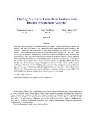
  • 10. with any quote being rejected and auctions with fewer than three quotes, leaving us with 841,552 request for quotations.28 Table 1 of Appendix C shows summary statistics for the whole period covered and for the new law, FZ#44 (2014–2016). The reserve price in requests for quotations is a maximum price that the winning bid cannot exceed in order for the auction to be considered valid. For requests for quotation this reserve price has lower than 500,000 rubles, or $8,700, as of the current exchange rate.29 In our sample, the mean reserve price is 213,507 rubles ($3,718).30 The mean winning bid is 157,850 rubles ($2,749),31 while the mean ratio of the winning bid to the reserve price is 73.3%.32 Figure 1 shows that the number of bids placed in the last hours before the deadline is large for all bidders; however, the winner tends to bid later asymmetrically more than the other bidders. Most of the extra density for the winner comes from the last minutes of the auction. The densities for the second, third, and fourth bidders are practically indistinguishable from each other. This is an exact pattern that we expect to see in the presence of bid leakage: even with a substantial share of bids placed in the last day, the winners tend to bid asymmetrically closer to the deadline, with a gap more pronounced in the last hours of the auction. In the next section we quantify this asymmetry between the winners and all other bidders, in order to detect and measure corruption. 28 The auctions without quotes do not provide any insights for our analysis. Neither do the rejected bids. We do not use the auctions with one or two bidders in our main analysis since we cannot employ our methods without observing a third bid. 29 Click here to update the exchange rate. 30 Click here to update the exchange rate. 31 Click here to update the exchange rate. 32 For more details on the reserve price distribution and the distribution of the winning bid one can resort to Appendix C. Panel A of Figure C1 shows that the distribution of reserve prices has almost a full support from 0 to 500,000 rubles. The empirical density of the reserve price is monotonically decreasing apart from the spikes at round numbers and especially on the maximum level of 500,000 rubles, and except for the neighborhood of 0. Panel B of Figure C1 shows that the winning bids have a similar distribution, but without a spike at 500,000 rubles. 9
  • 11. Figure 1: Hours to the Deadline for the Top Four Bidders 0 5 10 15 20 0.000.020.040.060.08 Last 24 hours; N = 112,525 Density Densities of Timing, Kernel Estimates By Bidder Rank Winners Runners−Up 3rd−Best 4th−Best Notes: Kernel density estimates for the timing of bids. Distance in hours to the deadline over the last twenty four hours. The densities are drawn separately for the winning bids, the runner-up bids, the third-best bids, and the fourth-best bids. Auctions with at least three bidders. The subsample is auctions with no bids placed within 15 minutes corridor from each other to control for artificial correlation coming from correlated bidding. FZ#44. Gaussian kernel with a normal optimal smoothing parameter is used. 4 Detecting Corruption We start this section by showing that corruption in the form of bid leakage is present in the data. We introduce an important assumption–an independence assumption. In the next subsection, we discuss why independence is likely to hold in our setting, and provide several tests for it. The inde- pendence allows us to measure corruption both for the whole sample and auctioneer-by-auctioneer. As Figure 1 shows, bids and timing of bids are correlated in a specific way, with winners placing their bids later in the auction. We argue that this is a result of corruption. An alternative explanation could be that there is correlation between timing and bidding decisions even absent corruption. For instance, more efficient bidders could place their bids later in the auction, while estimating the costs of the project, but this is implausible for the most of the contracts in our data. Yet another alternative explanation would be that bidders procrastinate in a specific way—e.g. with 10
  • 12. more efficient bidders procrastinating more. To rule out all of these alternative explanations, in the next subsection, we provide evidence against correlation of bids and timing absent corruption. For now, however, we just assume that bids and timing are independent, in a spirit of identification assumptions in collusion literature.33 Every bidder i in auction j is characterized by a pair (bij, tij), where bij a bid and tij, the timing of the bid. We omit the indices for the rest of the section. The independence assumption is, b ⊥ t (I) In this case, rejecting independence in the data is equivalent to accepting corruption. Next, we show that there is corruption in the form of bid leakage, but so far our tests are uninformative about the independece per se. We deal with this issue in the next subsection. In order to test for corruption, we exploit two specific violations of independence of bids and timing in the data that should be pronounced with bid leakage. The first is that without corruption, bidding last should not predict winning. We are testing the equality of probability of winning conditional on being the last one to bid and a probability of winning conditional on not being the last one to bid against the alternative of inequality. H0 : P[win|last] = P[win|not last] Test 1 We use the classical χ2 test for no association in contingency tables. Our case is simple, since it is a 2 × 2 contingency table consisting of two indicator variables–one for winning, and one for being the last in time. In practice, we implement this test by running an OLS regression of the indicator of winning on the indicator of being the last in time, and using Wald test from this OLS regression.34 33 See, for instance Porter and Zona (1993); Bajari and Ye (2003) for an example of how these restrictions are derived. 34 Anatolyev and Kosenok (2009) show that the classical χ2 test is asymptotically equivalent to the Wald test from OLS in this particular case. 11
  • 13. Figure 2: Hours to the Deadline for the Top Four Bidders 0 5 10 15 20 0.00.20.40.6 Cumulative Distribution of Timing, G(t|b) Last 24 hours; N = 109,333 CDF By Bidder Rank Winners Runners−Up 3rd−Best 4th−Best Notes: Empirical CDFs for the timing of bids. Distance in hours to the deadline over the last twenty four hours. The CDFs are drawn separately for the winning bids, the runner-up bids, the third-best bids, and the fourth-best bids. Auctions with at least three bidders. The subsample is auctions with no bids placed within 15 minutes corridor from each other to control for artificial correlation coming from correlated bidding. FZ#44. Apart from changing the conditional probability of winning, bid leakage shifts the timing of the winner closer to the deadline. This fact motivates our second test. Figure 2 illustrates the idea behind it. It shows the cumulative distribution functions of timing for winners, runners-up and other bidders. There is a large difference for winner and runner-up, while there is not much of a difference for the rest of the CDFs. If we denote the CDF of timing conditional on having kth rank in bids by G(t|b = b(k)), we want to test an equality of the distribution of timings for the winner and any of the other bidders (note that from independence they all should be the same). The H0 in this case is formulated as H0 : G(t|b = b(1)) = G(t|b = b(1)) Test 2 We test this hypothesis by a two-sample Kolmogorov-Smirnov test. 12
  • 14. Table 2 of Appendix C shows the results for the two tests above. Panel A runs Test 1 using Wald test from OLS of winning on being last. The difference in conditional probabilities of winning for the last bidder and for the non-last bidders is 0.096, and the p-value for the Wald test for equality of probabilities is less than 0.001. The fact that the last bidder is much more likely to win, strongly suggests the presence of corruption. We cannot accept the hypothesis of no corruption from Test I. Panel B of Table 2 implements Test 2 with a Kolmogorov-Smirnov test. We report the test statistics for Kolmogorov-Smirnov test for the equality of CDFs of timing for the winner, the runner-up, and the third bidder. All of the differences are significant at the 0.1% level as well.35 4.1 Independence and Alternative Explanations We fail to accept independence of bids and timing, and we interpret it as evidence of corruption. An alternative explanation could be that the independence fails even absent corruption, as in the examples with bidders collecting information, or bidders procrastinating. To test the independence without corruption, we need to construct a noncorrupt subsample. It is hard to build, since the noncorrupt subsample is fundamentally unobserved. However, with bid leakage we know the form of corruption, and hence we can derive such a subsample. We assume that the corrupt bidder waits until the last moment of the auction (or until all poten- tial bidders have placed their bids) and either undercuts the most competitive honest bid or places a high bid. Assumption 1. A corrupt bidder either wins the auction at the last moment or places a bid higher than the most competitive honest bid. For the first placebo test, we construct an artificial sample of auctions (A), discarding infor- mation on non-winning and non-last bids. We use Wald test from OLS as before. Note that now it is running a regression of being a runner-up on being the second-last, for the subsample of no winners and last bidders. The null hypothesis for this test is formulated as H0 : P[bidder second|second-last ∩ A] = P[bidder second|not second-last ∩ A] Test 1 against a two-sided alternative. For the second placebo test, we do not consider distribution functions of timings for the win- ners: H0 : G(t|b = b(j)) = G(t|b = b(k)), ∀j, k > 1 Test 2 35 To avoid noise on the right tail of the timing distribution, we keep only the auctions with t ≤ 72 hours. If we consider the whole sample, the differences will still be significant at the 0.1% level. 13
  • 15. Table 3 of Appendix C presents the results of our placebo tests. Panel A shows the results from the Wald test. We cannot reject no association, with a p-value still being less than 0.001, how- ever the difference in conditional probabilities is 7.4 times smaller in magnitude. In addition, the difference is negative, which implies that more efficient bidders do not bid closer to the deadline. In a similar spirit, Panel B repeats the Kolmogorov-Smirnov test for the equality of the second and the third CDFs (Row 3), the second and the fourth CDFs (Row 4), and the third and the fourth CDFs (Row 5). Two out of three differences are insignificant, one with p-value larger than 0.001, and another one with a p-value of 0.451. One implication of bid leakage and of Assumption 1 is that most of the results should be driven by the subsample of late bids. If the corrupt bidders are always among the winners and are the last bidders, the asymmetry in conditional probabilities should be more pronounced in the subsample of late bids. In contrast, there should not be much difference in the subsample where only early bids are placed. We define the “All Late” subsample as those bids that were placed within 60 minutes of the deadline. In addition, we define the “All Early” subsample, where all of the bids were placed at least five hours before the deadline. As an additional check, we concoct the “No Early” subsample, comprising auctions where at least one of the bids was placed less than five hours to the deadline. All of the subsample results are reported in Table 4 of Appendix C. When we run Test 1 for the “All Late” subsample, we find that the differences for this sub- sample are larger than for the whole sample; the test statistic is 0.153 (Row 1 of Table 4). This confirms the form of corruption. Next, we switch to the “All Early” subsample. The difference for this subsample is small 0.023 (Row 2 of Table 4). Next, we take the “No Early” subsample. If what we observe is indeed bid leakage, most of the difference should come from last-minute bidding, by the same logic that applied to the “All Late” subsample. As Row (3) of Table 4 shows, it is true that the difference the “No Early” subsample is large in magnitude (0.125). The results for auctions with more than three bidders are qualitatively similar. 4.2 Measures of Corruption Since we cannot reject independence given the data, Tests 1 and 2 can be modified to derive measures of corruption.36 One implication of the independence is that without corruption the probability of winning does 36 In addition, Appendix A discusses an alternative measure of corruption that is based solely on the information on the differences of bids between the winner and the runner-up, the runner-up and the third bidder, and so on. This method allows to measure corruption for auction data sets, where data on timing are not available. 14
  • 16. not depend on the timing. It is equal for all of the bidders. In an auction with K bidders, it is symmetrical and equal to 1/K. In the presence of bid leakage, the last bidder is always the winner, so this conditional probability is equal to one. Denoting the probability of corruption in an auction by α, the conditional probability of win- ning can be written as P[win|last] = α + 1 K (1 − α). Solving for α, one gets α = P[win|last] − 1/K 1 − 1/K . This is our first measure of corruption, αI. The second implication of the independence is that we can use the cumulative distribution func- tion of timings for non-winning bids as counterfactual for the CDF of timings without corruption. Namely, we can write G(t|b = b(1)) = α · G(t|b = b(1), corruption) + (1 − α) · G(t|b = b(1), no corruption). The independence implies that we can plug in for k > 1, G(t|b = b(1), no corruption) = G(t|b = b(k), no corruption) and then plug in G(t|b = b(k), no corruption) = G(t|b = b(k)). We also need to choose a parameterization for G(t|b = b(1), corruption), keeping in mind that with corruption the winner will bid close to the deadline. For now, we use a CDF that is discrete at 0, but we can also use a CDF of a uniform distribution on [0, ], where is relatively small compared to an average distance to the deadline. The results will be similar if we use uniform distribution instead of discrete. The interpretation is that the bid of the winner is by necessity placed at the deadline or in the neighborhood of the deadline. In this case, we can solve for α as follows, α = G(t|b = b(1)) − G(t|b = b(k)) 1t=0 − G(t|b = b(k)) . A sample analog of it depends on t. In practice, we implement the method as follows: we cut the sample to the last three days before the deadline, in other words, 72 hours. We are doing it to avoid finite sample bias arising from the skewness of the distribution of timings toward the deadline (see for example Figure 2). We also 15
  • 17. drop auctions where two bids were submitted together (within 15 minutes of each other).37 These two constraints leave us with around two-thirds of the initial sample. Next, we get the estimates of ˆα(t) for t = 0.5, 1, 2, and t = 5. We use an average of G(2) and G(3) for G(t|b = b(k)) to improve efficiency—we call this measure αII. We estimate a share of corrupt auctions from the first measure αI in Table 5 of Appendix C. Columns are split by subsamples by the number of bidders. The largest estimated share of corrupt auctions (9.6%) is for the three-bidder auctions (Column 1). Table 6 presents the results for the second measure αII with different comparison CDFs: either only the runner-up CDF or the average of the runner-up and the third, and with varying cutoff levels. The estimates vary from 8% to 12% and are all statistically significant at the 5% level.38 Panel B of Table 6 shows the results of the placebo tests, where the CDF of the winner is replaced by the CDF of either the runner-up or the third bidder. The placebo estimates are sometimes significant, but many of them are negative and insignificant. Overall, the estimates of the shares of corrupt auctions closely resembles the results from the first measure αI. These estimates allow us to provide some back-of-the-envelope calculations. To avoid weight- ing by the number of bidders we take ˆαII. Picking t = 1 as a medium cutoff we get αII = 0.108, or 10.8% of auctions are corrupt. If we multiply these numbers by the total number of contracts with three bidders and from FZ#44 we get that around 25,000 contracts are affected, with a total price of these contracts of $61 million. If we account for the auctions with two bidders and auctions from the first part of the study period (2011 to 2013) these numbers change to 383,000 contracts with a total value of $ 1.2 billion in six years. If we scale up these estimates to the total size of the government purchases—25% of GDP—2.7% of GDP is affected, although this figure is not very reliable, since corruption can take other forms in other types of government purchases. 4.3 Timing Response Another concern that we might have is that bidders react to corruption by adjusting their timing. Note that, to violate independence, and thus to threaten our tests, strategic response in timing needs to be correlated with the bid strength, or, in other words, with the efficiency of a bidder. We formally ruled out that this is the case in Table 3. In addition, as we discussed in Section 2 strategic timing response is highly unlikely with paper applications. However, it is more plausible with electronic auctions. Figure 3 shows the CDFs of timing for the auctions where only paper 37 In is a part of the sample, firms coordinate their bidding behavior by submitting their bids together or within a 15 to 20 minute interval. This can potentially bias our estimates in an unpredictable way. However, if we cut these simultaneous bids, we can prevent this from happening. 38 They are significant at the 1% level as well. 16
  • 18. submission was allowed (Panel A) and only electronic submission was allowed under FZ#44 (Pan- el B). The difference between CDFs for the non winners is more pronounced for the electronic submissions. The electronic submissions is a small part of the sample for FZ#4439 Thus, we are not concerned with the differential response in timing. Figure 3: Cumulative Distribution of Timing for the Top Four Bidders. Paper and electronic submission Panel A: only paper submission 0 5 10 15 20 0.00.20.40.6 Cumulative Distribution of Timing, G(t|b) Last 24 hours; N = 23,483 CDF By Bidder Rank Winners Runners−Up 3rd−Best 4th−Best Panel B: only electronic submission 0 5 10 15 20 0.00.20.40.6 Cumulative Distribution of Timing, G(t|b) Last 24 hours; N = 1,760 CDF By Bidder Rank Winners Runners−Up 3rd−Best 4th−Best Notes: The subsample is auctions with no bids placed within 15 minutes corridor from each other to control for artificial correlation coming from correlated bidding. Cumulative distribution functions for the timing of bids. Distance in hours to the deadline over the last twenty four hours. The CDFs are drawn separately for the winning bids, the runner-up bids, the third-best bids, and the fourth-best bids. Auctions with at least three bidders. Only the FZ#44. While we ruled out the differential response in timing, we still might be concerned that honest bidders adjust their timing independently of their bids. This does not affect our tests, but can bias our measures from the previous subsection. To address this issue, we compare the timing behavior of nonwinners in auctions, where our measures of corruption show high levels of corruption, and in those auctions, where measures of corruption, judging from αII is zero. Figure 4 depicts the CDFs of timing for winners, nonwinners for corrupt and noncorrupt auctions. 39 Less than 2% of bids had to be submitted only this way. 17
  • 19. Figure 4: Cumulative Distribution of Timing for Corrupt and Noncorrupt Auctioneers, Winners and Nonwinners 0 5 10 15 20 0.00.20.40.60.81.0 pKS12 = 0 , pKS23 = 0.018 , N win cor = 29,227 , N win hon = 3,254 G(x,f_h) Winner,hon.auc. >=2,hon.auc. >2,hon.auc. Winner,corr.auc. >=2,corr.auc. >2,corr.auc. Notes: The subsample is auctions with no bids placed within 15 minutes corridor from each other to control for artificial correlation coming from correlated bidding. Cumulative distribution functions for the timing of bids. Distance in hours to the deadline over the last twenty four hours. The densities are drawn separately for the winning bids, and other bids. Auctions with at least three bidders. Corrupt auctioneers are defined by ˆα ≥ 0.08, honest auctioneers are defined by ˆα ∈ [−0.01; 0.02] As one can see from the graphs, while the difference between winning CDFs is large by con- struction, there is practically no different for the nonwinning CDFs of timing. The Kolmogorov- Smirnov test that we run show that the difference is not significant. Thus, we can rely on our measures αI and αII. 5 The Model How does corruption affect prices? In Section 4, we used the tests to detect the patterns in the data that are indicative of corruption. Then we applied the measures to estimate the share of corrupt auctions. Naturally, one wonders how bid-leakage corruption affects the final prices of contracts. The final prices of contracts serve as a convenient measure of government effectiveness in the 18
  • 20. procurement setting (see for example Bandiera, Prat, and Valletti 2009; Lewis-Faupel, Neggers, Olken, and Pande 2014; Best, Hjort, and Szakonyi 2017). To examine the channels through which corruption affects prices, we model the bidding behavior of an honest bidder. In our model, corruption effectively reduces the level of competition in an auction. Specifical- ly, the direct effect of corruption is proportional to a change in expected prices, when competition in the auction is reduced by one bidder.40 As we see from the model, an additional channel ex- ists through which corruption affects the equilibrium price—the response of honest firms. Under certain conditions on the distribution of costs, honest firms can place lower bids than without cor- ruption. In other words, with corruption they bid more aggressively. This reduces the expected price of the contract, in contrast to the direct effect. We show in a stylized example that this indirect effect can be strong enough for corruption to reduce the overall expected prices. Note that we use the results from Section 4 and directly assume that the independence holds. This allows us to concentrate only on the bidding decision, avoiding modeling the decision on the timing of bids and the response of honest bidders with adjusted timing. We model the bidding decision as a standard first-price sealed-bid procurement auction with independent private costs. We want to point out several facts: (1) there is an equilibrium in mono- tone bidding strategies; (2) the curvature of the distribution of costs determines whether honest bidders bid more aggressively then they would without corruption; (3) the expected price implica- tions of this behavior depend on the shape of the costs distribution, and therefore, the price effect of corruption is an empirical question. The public body is buying a good or a service from K buyers, where K is a fixed number of bidders.41 The cost of bidder is an independent draw from a CDF F on the interval [0, ¯c]. All the players are risk-neutral. Corruption takes the following form: an auctioneer runs a corrupt auction with a probability α. If the auction is corrupt, one of the bidders learns the bids of other bidders and can place her bid guided by this information. We assume that if upon learning other bids the corrupt bidder does not find it profitable to win the auction, she bids above the most competitive honest bid. Another assumption is that corrupt bidders are drawn from the same distribution than honest bidders.42 Assumption 3 summarizes all of the conditions for our analysis. 40 The change in expected price in our context is the same as the change in expected revenue for value auctions. Corruption can also lead to an inefficient outcome. The outcome of the auction is inefficient, when the corrupt firm has higher costs, than the most efficient honest firm, but it still wins the auction. 41 We relax this assumption in the estimation procedure in Section 7. 42 We acknowledge that allowing asymmetries between honest and corrupt bidders, and testing for them is also possible in this setting, but it is not our goal. More important, if we allow for different cost distribution for corrupt and honest bidders, the model below is not identified nonparametrically and requires strong parametric assumptions 19
  • 21. Assumption 2: A. Independence holds. B. The costs c are i.i.d draws from F(·), same for both types of bidders. C. A corrupt bidder bids above the most competitive honest bidder, when it is not profitable for her to win the auction. An honest bidder in this case maximizes the following function: ν(b, c, α) = (b − c)(1 − G(b))K−2 ((1 − α)(1 − G(b)) + α(1 − F(b))), where G(b) = F(φα(b)) is the CDF of bids. φα(b) is an inverse of a bidding strategy. Note the α index. It stressed that bidding behavior depends on the extent of corruption measured by the probability of an auction being corrupt. The equilibrium is given by the first-order condition, c = b − χ(α, b) := = b − (K − 2)g(b) 1 − G(b) + (1 − α)g(b) + αf(b) (1 − α)(1 − G(b)) + α(1 − F(b)) −1 . (2) Note that for α = 0, this boils down to regular FOC of a first-price sealed-bid auction. Our setting resembles the one studied in Arozamena and Weinschelbaum (2009), with two differences. First, we study the procurement setting. As a result, the conditions on the underlying distributions of costs for existence of equilibrium, aggressive behavior of honest bidders, and for the revenue implications are slightly different. Second, is that we allow for α ∈ (0, 1], while their analysis is only for the case of α = 1. That is, auctions are always corrupt in their setting. We provide all of the technical results that differ from proofs of Arozamena and Weinschelbaum (2009) in Appendix B. Definition 1: Log-concavity of survival function. Survival function is defined as 1 − F(x). We assume that it is log-concave. Note that it means that h(x) = f(x) 1−F(x) (the hazard function) is increasing.43 We argue in Appendix B that log-concavity is sufficient for there to exist a symmetric equilibri- um characterized by the solution to the differential equation in the FOC (2), and that the differential for identification. 43 A broad class of distributions satisfy log-concavity of survival function, e.g., uniform, normal, logistic, extreme values, exponential, Laplace, Pareto, chi-squared, and chi. Power function distribution satisfies it for a value of the main parameter larger than 1. For the value of the parameter less than for power distribution and for Pareto distribution, the survival functions are not log-concave. However, one can compute the bid functions directly in both of these cases. For a detailed treatment of log-concavity and its applications, see Bagnoli and Bergstrom (2005). 20
  • 22. equation (2) has a strictly increasing solution. Proposition 1. If the survival function is log-concave, then (2) defines an equilibrium with corruption. If corruption makes the bidders more aggressive, for the same value of the costs the bid will be lower with corruption. In other words, by monotonicity, the costs have to be higher to achieve the same bid level. Formulating it in terms of the FOC (2), more aggression occurs when χ(α, b) < χ(0, b). Proposition 2 establishes whether there is more, or less, aggression with corruption. Proposition 2. If w(x) = h−1 (x) = 1−F(x) f(x) is strictly convex, there is more aggression, i.e., χ(α, b) < χ(0, b). If w(x) is strictly concave, there is less aggression, i.e., χ(α, b) > χ(0, b). If w(x) is linear then corruption does not affect bidding behavior.44 45 We illustrate aggression in Example 1. Example 1: Power distribution and aggression. Assume that costs are distributed according to power law, that is F(x) = xθ , θ > 0, x ∈ [0, 1]. For simplicity we consider a case with only two bidders K = 2, where the auctioneer is completely corrupt α = 1 or completely honest α = 0. Solving the differential equations from the FOCs, we get a bidding strategy in an honest auction: β0(c) = θ 1 + θ 1 − cθ+1 1 − cθ . In a corrupt auction, a bid function is defined implicitly through φc (b): φα=1(b) = θ + 1 θ b − 1 θ b1−θ . Figure 5 shows these bid functions for two cases: θ = 0.5 and θ = 2 (Panels A and B, respectively). One bid function being below another means more aggression in this case. The critical value for θ is 1 (uniform distribution). For θ = 1, the distribution is uniform and corruption does not change the bidding behavior of the participants. If θ > 1, corruption makes honest bidders more aggressive, and vice versa, if θ < 1, corruption makes honest bidders less aggressive. 44 Note that it is true for Pareto distribution, F(c) = 1 − c−γ , γ > 0, which does not have a log-concave survival function. However, the bid functions can be derived directly, and α does not affect them. 45 In Appendix B, we show that Proposition 2 holds for α ∈ (0, 1). 21
  • 23. Figure 5: Bidding Behavior with and without Corruption Panel A �������� θ 0.0 0.2 0.4 0.6 0.8 1.0 0.3 0.4 0.5 0.6 0.7 0.8 0.9 1.0 Honest Auction Corrupt Auction Panel B �������� θ 0.0 0.2 0.4 0.6 0.8 1.0 0.3 0.4 0.5 0.6 0.7 0.8 0.9 1.0 Honest Auction Corrupt Auction Notes: Panel A: Less Aggression with Corruption, θ = 0.5. Panel B: More Aggression with Corruption, θ = 2 Proposition 2 shows that under fairly general assumptions the expected prices paid to the honest procurers are lower than under corruption. This equilibrium response weights with the direct effect of corruption, so the price implications are potentially ambiguous. Aggression on its own is not enough to make a statement about the expected price. To illustrate this point, we show how the expected price changes with corruption. Propensity for corruption Corrupt auctioneer No Corruption p = b(I,K) Ep = E[b(1,K)|φ0 ] Corruption happens p = ccorrupt = b(I,K−1) Ep = E[b(1,K−1)|φ1 ] actual number of bidders is K Corruption does not happen p = b(I,K−1) Ep = E[b(1,K−1)|φ1 ] actual number of bidders is still K α 1 − α c < b(I,K−1) c > b(I,K−1) The graph above illustrates that even if an auction is corrupt, the corrupt bidder can abstain. 22
  • 24. This will effectively bring the corrupt auction with no corruption to an auction with K−1 bidders.46 The expected price is given by the following expression: E[price] = E[b(1)] = α · E[b (α) (1,K−1)] + (1 − α) · E[b (0) (1,K)]. This expression can be also presented as follows: E[price] = α · (K − 1) · b · gα(b)(1 − Gα(b))K−2 db + (1 − α) · K · b · g0(b)(1 − G0(b))K−1 db. Rewriting it once again in terms of the direct and indirect effects, we get, E[price] = K · b · g0(b)(1 − G0(b))K−1 db + α · (K − 1) · b · gα(b)(1 − Gα(b))K−2 db − K · b · gα(b)(1 − Gα(b))K−1 db + inflating, direct effect > 0 K · b · gα(b)(1 − Gα(b))K−1 db − K · b · g0(b)(1 − G0(b))K−1 db deflating, indirect effect > 0 . The integrals in this expression can be calculated explicitly for some distributions or evalu- ated numerically. We continue with Example 1 to illustrate the changes in expected prices with corruption. Example 1: Continuation. Without corruption, we need to find E[price|α = 0] = E[b0 (1,2)] = 1 0 β0(c)f(c(1,2)dc = 1 0 2θ2 1 + θ (cθ−1 − c2θ )dc = = 2θ2 1 + θ cθ θ − c2θ+1 2θ + 1 1 0 = 2θ 1 + 2θ . With corruption, we need to find E[price|α = 1] = E[b1 (1,1)] = 1 0 θcθ−1 β1(c)dc = {β1(c) = z, dc = θ + 1 θ − 1 − θ θ z1−θ dz, z(0) = (1 + θ)−1/θ } = 46 The auction can still be a K-bidder auction, but with one high bid being unimportant. Moreover, if we follow the equilibrium choice at the beginning of the section, this bid will still be from the same distribution as the other honest bids. 23
  • 25. θ 1 z(0) θ + 1 θ z − 1 θ z1−θ θ dz + 1 z(0) z1−θ θ + 1 θ z − 1 θ z1−θ θ−1 dz . This expression needs to be evaluated numerically. Table 7 shows how both expected prices vary with θ. They are approximately equal for θ = 2, and the expected price is lower for θ > 2. This example shows that corruption can reduce expected prices. Note that there is no one-to-one correspondence between aggression and the expected price. The aggression is not high enough for 1 < θ < 2 to have a negative indirect effect on prices. In the empirical sections that follow, we examine whether there is more aggression with corruption and we estimate the magnitude of the direct and indirect effects. 6 Reduced-Form Estimates of Price Differences In this section, we bring the results of the model to the data. Our first exercise is to examine the correlation of our measures of corruption with the prices of the contracts. To do so we need to first measure corruption by auctioneers and bidders. Our second exercise is to decompose the effect of corruption into direct and indirect components, which allows us to test our model. We start by normalizing prices and including regional fixed effects, goods and services cate- gories fixed effects, year fixed effects, and month fixed effects; in line with both the literature on inefficiencies in procurement (Bandiera, Prat, and Valletti, 2009; Best, Hjort, and Szakonyi, 2017) and the literature on observed heterogeneity in auctions (Haile, Hong, and Shum, 2003). We can still be concerned that omitted variables associated with corruption could directly affect prices. Hence, we also control for the type of procedure (paper or electronic), for the type of public body, for the number of bidders, and for quintiles of the reserve price.47 We regress the log of prices and the log of bids on the controls and on the measures of corruption. Finally, we can be concerned that bidders, who participate in auctions with corrupt and non- corrupt auctioneers are fundamentally different from each other. One main difference is selection based on in their costs. We address this selection problem by including bidders fixed effects. Bid- ders fixed effects allow us to control for any unobserved heterogeneity in prices coming from the type of the bidder. Since we fix the identity of the bidder, the estimates compare the behavior of the same bidder with corrupt and noncorrupt auctioneers.48 A potential remaining concern is that an unobservable characteristic of auctioneers, which causes higher prices, and which is positively correlated with corruption, can bias our estimates upward. It is very unlikely that such a variable exists, because we control for the the choice of 47 We use 86 regions in our sample, and 88 first-level categories of goods and services. 48 We also controlled for the number of bidders in the auction, and it did not change the results. 24
  • 26. the good, we control for differential entry of bidders, and for the reserve price, conditional on the choice of good. In the second exercise, we want to understand whether honest bidders indeed bid more ag- gressively, when they expect corruption to happen, and we want to estimate the magnitude of this effect. In order to do so, we include measured corruption of the auctioneer, measured corruption of the bidder, and the interaction between the two in the price regression. We expect that for honest bidders, corruption of auctioneers will have a price-reducing effect, while for corrupt bidders it will inflate the price, and the direct effect will dominate. We can also include bidders fixed ef- fects to control for bidder heterogeneity and estimate the interaction between the fixed effects and corruption as an additional check. 6.1 Measuring Corruption for Auctioneers and Bidders In this Section, we allow the level of corruption—α—to vary between auctioneers and bidders. Thus, we can estimate α for different auctioneers by using either αI or αII. Likewise, we can estimate α for a bidder.49 Once we have measures of corruption for the auctioneer and for the bidder, we can correlate those with prices of the contracts. To implement this, we need to have enough power to estimate α for a participant. That is, an auctioneer or a bidder should have participated in enough auctions to have enough power to estimate α.50 When we keep the frequent participants, we are left with 3,615 auctioneers and 5,043 bidders. Figure 6 shows the distribution of α. Most of the mass is positive, in line with the positive aggregate estimates of α in Section 4.51 49 Note that corruption of the bidder is not a structural parameter of the model. Still, it will be informative of the asymmetry of winning probabilities for a given bidder, and hence informative on how often she was involved in corruption. 50 We cut the sample based on the following constraint: a bidder should have bids placed in at least 200 auctions; at least 30 of which had three or more bidders. The auctioneer should have at least 200 auctions, at least 30 of which had three or more bidders. 51 Moreover, the median and mean values of the estimates for the subsamples of frequent participants are 0.074 and 0.082 respectively, which is in line with the estimates for the whole sample in Section 4. 25
  • 27. Figure 6: Distribution of ˆα for Auctioneers and Bidders Panel A: Auctioneers01234 KernelEstimate -.5 0 .5 1 α of auctioneers N=3615 Panel B: Bidders 01234 KernelEstimate -1 -.5 0 .5 1 α of bidders N=5043 6.2 Price Differences Once we have the measures of corruption for auctioneers and bidders, we want to study how prices of contracts are changing in auctions with bid leakage. First, we run the following regression: log(priceaig) = θ0 + θ1 · αa + θ2 · Xai + µg + νaig, (3) where a indexes auctioneers and i is an auction index. Xai is a set of control variables, µg are goods fixed effects. Note that we do not observe corruption directly; that is, we cannot use αa, so we have to use our estimates of corruption ˆαIa. The coefficient of interest in (3) is θ1. The interpretation of it is partial correlation of corruption and prices. We start by examining raw and partial correlations in Table 8, Columns (1) and (2), respectively. Both estimates are positive and significant, indicating that an increase in corruption is correlated with an increase in prices. Even though we included goods fixed effects, and the set of controls also includes regional fixed effects, years and months fixed effects, a dummy for change in the regulations, and a dummy for a number of bidders in the auction, we are still cautious about interpreting it as a causal effect. Instead, we add bidders fixed effects for each bidder ξb, and then rerun (3) as log(priceaigb) = ˜θ0 + ˜θ1 · αa + ˜θ2 · Xai + ˜µg + ξb + ˜νaigb, (4) The resulting coefficients of interest are in Column (3) of Table 8. Including bidders fixed effects only increases the coefficient, which is now equal to 0.275. 26
  • 28. We get a back-of-the-envelope calculation for price changes from it. Public bodies with dif- ferent levels of bid leakage pay different prices for the contracts. A public body with ˆα = 0.25, which corresponds to the 97th percentile, ends up paying 7.1% higher prices than a public body with no bid leakage. If we shift all of the auctioneers with positive estimates of corruption to no corruption, that is, from ˆα = 0.103 to zero, the savings are still sizable: 2.9%. 6.3 Testing the Model The estimates in Table 8 pool the direct and indirect effects of corruption from the model. We want to test the extent to which the indirect effect of corruption contributes to the price estimates. To do so, we note that if we fix an identity of a bidder to be an honest bidder, she should reduce her bid when she faces a corrupt auctioneer. At the same time, if it is a corrupt bidder facing a corrupt auctioneer, the prices and the bids should both go up. We test it by running following regressions: log(bidaigb) = β0 + β1 · αa + β2 · αb + β3 · αa · αb + β4 · Xai + ηg + aigb, (5) log(priceaigb) = ˜β0 + ˜β1 · αa + ˜β2 · αb + ˜β3 · αa · αb + ˜β4 · Xai + ˜ηg + ˜aigb, (6) where b indexes bidders, and the rest of the notations are as before. The coefficients of interest in the regressions are β1, β2, and β3 for the first regression, and ˜β1, ˜β2, and ˜β3 for the second one. If our model is correct, absent bidder corruption, auctioneer corruption will lead to more aggression—β1 < 0. If a corrupt bidder and a corrupt auctioneer face each other, the bid should go up on average due to a direct effect on prices—β3 > 0. The direct effect of corruption will be a linear combination of β1, β2, and β3. We run the equations above for two subsamples. The first one involves auctioneers and bidders with higher than median participation.52 The second subsample is complementary to the first one. The predictions should hold only if players bid according to the equilibrium described in our model. We expect that they behave as in the model in the subsample of frequent participants. We start by estimating the equations (5) and (6) for the subsample of frequent participants, and we report the results in Table 9. Table 9 shows the results for both bid-level (5) and price-level (6) regressions for frequent participants. Columns (1) and (2) show a raw and partial correlation of the logarithm of bids and the corruption of the auctioneer. Both of them are positive, statistically significant, and of the same order of magnitude as they are for the prices for the whole sample. The coefficients for prices in 52 Specifically, these are auctioneers that had at least 685 bids placed in their auctions and participants that put their bids in at least 361 auctions. 27
  • 29. Columns (6) and (7) are very similar, though the partial correlation is insignificant. Column (3) shows our baseline specification for the bids. Both of the baseline coefficients for corruption of auctioneers and bidders are negative and significant ˆβ1, ˆβ2 < 0, while the interaction term is positive and significant ˆβ3 > 0, as predicted by the model. One way to interpret the magnitude is to see how moving from no corruption αa = 0 to αa = 0.25 changes the bids. Such a change increases the bids by 10.5%. If we fix the level of corruption for the bidder and the auctioneer as equal to each other (αa = αb), there is a nonzero level of corruption that minimizes the price. This level is 0.087, close to the median in the sample, but still below the mean for the auctioneers that have a positive level of corruption, 0.103. If instead of moving from α = 0.25 to α = 0, we move from α = 0.103 to α = 0.087, the bids will drop by 0.12% of the initial level. While we treat Column (3) as our main specification for (5), an unobservable characteristic of the contract can exist that is not captured by geography, type of good or service, time, type of public body, law, or competition measured by the number of bidders. One characteristic that may capture this unobservable is the reserve (maximum) price of the contract. The main caveat here is that we cannot directly control for the log-reserve price, because it can be affected by corruption directly and thus is a bad control. Corrupt public bodies can inflate the reserve price, and so including it in the regression will be over controlling (see Angrist and Pischke, 2008; Maccini and Yang, 2009). Moreover, the correlation between the bid and the reserve price is 0.95, with an OLS coefficient close to 1, so including it on its own will drain all of the variation. However, we control for the quintiles of the reserve price to address unobserved variables related to the size of the contract and potentially other unobserved characteristics of the contract. Column (4) of Table 9 shows the results controlling for the quintiles of the reserve price. The coefficients get smaller in magnitude but preserve similar patterns as in Column (3). Moreover, the coefficient on bidder corruption shrinks by a factor of two and is only significant at the 10% level. The richness of our data allows us to pin down all of the unobserved variation coming from the bidder side by directly including bidders fixed effects, instead of including the measure of cor- ruption αb. The magnitude of the effects in Column (5) shrink, but they remain both economically and statistically significant.53 53 Note that the coefficient on ˆαb is not identified with bidders fixed effects, however the coefficient on the interaction term ˆαb · ˆαa is identified and it is our quantity of interest in Columns (5) and (10). One can be potentially concerned that it hides a heterogeneity in bidder effect. In addition, in Appendix C, Figure C2 we show the distribution of the interaction terms of bidder fixed effects and corruption of the auctioneers. As can be seen from the graph, those coefficients are predominantly positive. 28
  • 30. We tested our model and measured the effects on the average bid, rather than the effective final prices of the contract. Columns (6—10) of Table 9 repeat the analysis for final prices (as in equation (6)). The sizes of the coefficients in Columns (8) and (9)—with and without reserve price controls—are larger in magnitude than in corresponding Columns (3) and (4) and are in line with the model. Bidders fixed effects drain a lot of the variation from the sample and make the coefficients imprecisely estimated, keeping the signs of the coefficients in line with the model (Column 10). Table (9) provides a basis for another important back-of-the-envelope calculation. We use the estimates in Column (8) to derive them. Moving from no corruption to α = 0.25 for both bidders and auctioneers increases prices by 15.0%. At the same time, prices are minimized for the level of corruption α = 0.053. Moving from the average of auctioneers with positive corruption 0.103 to this minimum level reduces prices by 0.4%. The results are entirely different for the subsample of infrequent participants, as reported in Table 10. The coefficient on auctioneer corruption is smaller in magnitude compared to Table 9 and positive. All of the interaction terms are insignificant, whether we take the bids (Columns 1—5) or the prices (Columns 6—9). The exception is Column (10), with a negative and signif- icant coefficient on the interaction term. If we do the back-of-the-envelope calculations for this subsample, switching from zero corruption to α = 0.25 increases prices by 9.8%, while moving from α = 0.103 to zero corruption reduces prices by 5.3%. 6.4 Comparison to Existing Estimates of Corruption Before proceeding to structural estimation in the next section, we compare our baseline estimates with the estimates of procurement corruption in the existing literature. Our baseline effect on prices is 7.1% if we switch from high corruption to zero corruption, and it is 2.9% if we reduce corruption for all of the auctioneers who have a positive measure of corruption. Both of the numbers are lower than the results from similar contexts in Di Tella and Schargrodsky (2003) and Bandiera, Prat, and Valletti (2009), but not drastically so. The first paper estimates the effect of the crackdown on corruption on procurement prices in Argentinean hospitals and finds and effect of 10%, while the second paper estimates active waste in Italian procurement, with a corresponding price difference of 11%. Other papers (Ferraz and Finan, 2011; Olken, 2006, 2007; Reinikka and Svensson, 2005) study diverted funds in Brazilian local expenditures, loss in subsidized rice and missing road con- struction expenditures in Indonesia, and diverted education funds in Uganda—show loss estimates ranging from 9% to 24%. Our estimates are lower, but again not dramatically so. None of the existing studies decompose the effect of corruption into direct and indirect effects. 29
  • 31. For subsample of frequent bidders, the indirect effect shifts the optimal corruption level from zero to a positive number. In this specific subsample, going from the mean level to the optimal level will reduce prices by 0.4%, but completely eliminating corruption will raise prices. 7 Identification and Estimation of the Structural Model Reduced-form results show that corruption increases prices for the whole sample, with an im- portant heterogeneity in the results. For the subsample of frequent auctioneers and bidders an indirect price-reducing effect of corruption is present. We want to document that these reduced- form changes come from the model in Section 5. Our main objects of interest are the equilibrium bid functions for honest bidders. We want to establish that bid functions of honest bidders, when they face corrupt auctioneers shift downward compared to bid functions of honest bidders, when they face honest auctioneers. That is, for the same level of costs, honest firms in corrupt auctions reduce their bids. To provide preliminary evidence on the extent of the equilibrium response of honest bidders, we use our model of bidding behavior with corruption and incorporate the identification results of Guerre, Perrigne, and Vuong (2000). While our main empirical contribution from the previous sections to do not rely on the first-order condition, we need to use the FOC from Section 5 to estimate the bid functions. The first-order condition with corruption is c = b − χ(α, b) = b − (K − 2)gα(b) 1 − Gα(b) + (1 − α)gα(b) + αf(b) (1 − α)(1 − Gα(b)) + α(1 − F(b)) −1 . (2) As before, f and F are the density and the cumulative distribution function of the costs. We modify notation to stress that the distribution of bids depends on the level of corruption; we use a notation Gα and gα with α index. In this case, the distribution of bids without corruption is G0 (with the probability density function g0). The FOC implicitly defines the central quantity of interest—the bid function βα(c), which depends on the level of corruption α. To estimate this bid function, we need to observe and estimate the distributions F and Gα, as well as the level of corruption α. We proceed in four steps. (1) First, we measure corruption for all auctioneers and bidders who have enough data. This gives us the measures ˆαa and ˆαb as in Section 6. 30
  • 32. (2) Second, we choose the subsample of honest bidders ˆαb ≈ 0 and honest auctioneers ˆαa ≈ 0. Note that in this noncorrupt subsample, the FOC boils down to the standard first-price sealed-bid auction FOC, with χ(α, b) = (K − 1)g0(b) 1 − G0(b) −1 . Hence, all of the identification and estimation results from Guerre, Perrigne, and Vuong (2000) hold. Thus, we can estimate the distributions G0, g0. Then, we can generate pseudo-costs ˆc, and estimate the distribution of F, and density f using the generated pseudo-costs. (3) Third, we vary α for auctioneers, while keeping ˆαb ≈ 0. That is, since the FOC holds only for honest bidders, we want to examine their behavior. At the same time, we want to study what happens when we move the level of corruption for the auctioneer. This allows us to estimate Gα for a fixed level of corruption α simply from the empirical CDF. Likewise, we get consistent estimates for the density of bids gα. (4) Fourth, we already have all of the estimates ˆF, ˆf, ˆgα, ˆGα, and ˆαa, which we can plug into FOC with corruption to get ˆχ = ˜χ( ˆF, ˆf, ˆGα, ˆgα, ˆαa, ˆp; b). Once we do it, we immediately have the estimate for the bid function. Theorem 1 of Guerre, Perrigne, and Vuong (2000), with b − χ(α, ·) instead of φ0(b), provides us with the identification result. Plug-in estimators will be consistent in this case. (4’) We also employ an alternative approach: since we assumed that the distribution of costs is the same for any α; we can solve Gα(b) = F(φα(b), where φ is an inverse bid function. This equation can be solved by inverting ˆF. The resulting estimate for the inverse bid function will be ˆφα(b) = ˆF−1 ( ˆGα(b). 7.1 Practical Considerations In the previous subsection, we held the number of bidders fixed at K. Ideally, we want to control for the number of bidders, which varies from auction to auction. We do assume that bidder entry happens exogenously and the distribution of the number of bidders is geometric with parameter p on {3, ...}. Note that p is not a function of α; that is, corruption on its own does not discourage bidders from participating. Although the assumption might seem strong, the average number of bidders does not differ for auctions with different measured α of auctioneer. In the case of random entry, expected profit changes to ˜Π(b) = (b − c)((1 − α)(1 − G(b)) + α(1 − F(b)))EK[(1 − G(b))K−2 ]. 31
  • 33. For geometric distribution, the FOC becomes54 c = b − ˜χ(α, b, p) = b − (1 − α)gα(b) + αf(b) (1 − α)(1 − Gα(b)) + α(1 − F(b) + gα(b) 1 − Gα(b) + (1 − p)gα(b) 1 − (1 − p)(1 − Gα(b)) −1 (2 ) The last component of the modified FOC is the entry component. We estimate ˆp = 0.49 and use it throughout. We assumed that auctions are homogeneous when we outlined the structural model. In the estimation, we relax this assumption and follow a first-stage-regression approach common in the literature (Haile, Hong, and Shum, 2003; Bajari, Houghton, and Tadelis, 2014; Asker, 2010a). At the first stage, we project the logarithms of bids on the covariates. Note, that it is only possible if the observed heterogeneity enters the valuations in a multiplicatively separable way. Once we do the projection, we run the rest of the analysis with the exponentiated residuals. For consistency, we use the same covariates as in Section 6; that is, dummy variables for regions, for types of goods and services, for years and months, a dummy for FZ#44, and a dummy for whether the public body is a medical or educational institution. 7.2 Results We implement the procedure from the previous subsection. In order to estimate the fundamentals of the model, we need to pick cutoffs. First, we pick a subsample of auctioneers and bidders who took part in a sufficient number of auctions, as in Section 6. We concentrate only on the bidders with low αb (below the median ≤ 0.06). Next, for estimating the pseudo-costs in noncorrupt auctions, we need to pick the auctioneers with no corruption. We take 30% of auctioneers with the lowest αa to estimate the pseudo-costs distribution F. Once, we have the estimate ˆF, we estimate Gα auctioneer-by-auctioneer. To illustrate our results, we choose several auctioneers with a sufficient number of auctions and with different values of ˆαII ≈ 0. The table below illustrates our choice. Number of Auctions 4,175 2,266 2,333 1,980 568 572 ˆαa 0.05 0.13 0.21 0.08 0.00 -0.00 Figure 7 shows the resulting estimates for the bid functions. The first four panels show the results for the auctioneers with a positive level of corruption. In three of four cases, corruption 54 The last multiplier in this expression transforms to EK[(1 − G(b))K−2 ] = p(1−G(b)) 1−(1−p)(1−G(b)) . We take logarithms of the expression and we maximize it with respect to b. 32
  • 34. moves the bid functions toward more aggression: in one case, it is inconclusive what happens to the bid functions. Still, the evidence points to more aggression. For auctioneers with a low level of corruption, there is no evidence of more aggression, which is also in line with the mechanisms from the model. 33
  • 35. Figure 8: Bid Functions for Different Auctioneers, FOC Method 34
  • 36. Estimating the model auctioneer-by-auctioneer suggests that we do observe more aggression, but the results are not robust across auctioneers. Finally, we pool auctioneers whose level of αII is in a neighborhood of 0.02 of the median value, α = 0.09, and rerun both of the methods. We plug in α = 0.09 directly in the FOC. Panel A of Figure 9 shows the results. While parts of the bid function lie below the bid function for no corruption, some parts are above the no-corruption bid function. We also check what happens when we invert the CDFs at step 4, instead of plugging the es- timates into the FOC with positive corruption. The resulting estimates from the CDF method are shown in Figure 9, Panel B. The bid function is below the no-corruption case, and in line with more aggression. To sum up, we developed a way to test a model of first-price sealed-bid auctions with bid- leakage corruption, and we show that the estimates of bid functions suggest that the indirect effect of corruption is at play. Figure 9: Bid Functions for No Corruption and for Pooled Auctioneers Panel A: FOC Panel B: CDF method 8 Conclusion In this paper, we develop methods to measure corruption focusing on timing of bids. These meth- ods allow us to document large-scale bid-leakage corruption prevalent in Russian procurement 35
  • 37. auctions. From 2011 to 2016, the cumulative value of the affected contracts was as high as $1.2 billion. The regression of prices on measures of corruption suggests that eliminating bid leakage could have lowered prices by 2.9%. For our subsample of frequent auctioneers and bidders, an- other effect of corruption—the indirect effect—lowered the prices paid to the honest bidders, who adjusted their bidding behavior to attenuate corruption. Our paper is the first to provide estimates of this type of corruption empirically, and to estimate the effects of such behavior on prices. We also stress that the change in equilibrium behavior of honest bidders is important, when the monitoring authorities eliminate bid leakage. We still can discuss several policy implications. The first involves changing the way that con- tracts are distributed. Running an open auction or a second-price sealed-bid (Vickrey) auction could help remedy bid-leakage corruption. The equilibrium outcomes of these auctions should make participants bid their true costs. Therefore, the preferred bidder and the honest bidders will behave similarly, which would, at first glance, solve the problem of bid leakage. However, open auctions and Vickrey auctions both have problems of their own; both can facilitate collusion be- tween bidders (Robinson, 1985). In the environment of Russian procurement, collusion can ensure even larger losses. In addition, Vickrey auctions come with privacy concerns: auctioneers can in- vite shill bidders to reduce the margin between the lowest bids. Moreover, once a bidder reveals her true costs, the auctioneer may alter his behavior in the future.55 As opposed to changing the auction mechanism, employing technological advancements is likely the best way forward. First, introducing an encrypted electronic system could reduce bid leakage. Second, tracing the timing of bids to monitor auctioneers could prove useful in targeting this type of corruption. 55 For a discussion of why Vickrey auctions are rarely used, see Rothkopf, Teisberg, and Kahn (1990). 36
  • 38. References Anatolyev, S. and G. Kosenok (2009). Tests in contingency tables as regression tests. Economics let- ters 105(2), 189–192. Angrist, J. D. and J.-S. Pischke (2008). Mostly harmless econometrics: An empiricist’s companion. Prince- ton university press. Arozamena, L. and F. Weinschelbaum (2009). The effect of corruption on bidding behavior in first-price auctions. European Economic Review 53(6), 645–657. Asker, J. (2010a). Bidding rings. The New Palgrave Dictionary of Economics 4. Asker, J. (2010b). A study of the internal organization of a bidding cartel. The American Economic Re- view 100(3), 724–762. Athey, S., J. Levin, and E. Seira (2011). Comparing open and sealed bid auctions: Evidence from timber auctions*. Quarterly Journal of Economics 126(1). Bagnoli, M. and T. Bergstrom (2005). Log-concave probability and its applications. Economic Theory 26(2), 445–469. Bajari, P. and A. Hortacsu (2003). The winner’s curse, reserve prices, and endogenous entry: Empirical insights from ebay auctions. RAND Journal of Economics, 329–355. Bajari, P., S. Houghton, and S. Tadelis (2014). Bidding for incomplete contracts: An empirical analysis of adaptation costs. The American Economic Review 104(4), 1288–1319. Bajari, P. and L. Ye (2003). Deciding between competition and collusion. Review of Economics and Statis- tics 85(4), 971–989. Baldwin, L. H., R. C. Marshall, and J.-F. Richard (1997). Bidder collusion at forest service timber sales. Journal of Political Economy 105(4), 657–699. Baltrunaite, A. (2016). Political finance reform and public procurement: Evidence from lithuania. Bandiera, O., A. Prat, and T. Valletti (2009). Active and passive waste in government spending: Evidence from a policy experiment. The American Economic Review, 1278–1308. Banerjee, A., E. Duflo, C. Imbert, S. Mathew, and R. Pande (2014). Can e-governance reduce capture of public programs? experimental evidence from a financial reform of indiaâ ˘A´Zs employment guarantee. economics. mit. edu/files/10557 (accessed July 1, 2015). Best, M. C., J. Hjort, and D. Szakonyi (2017). Individuals and organizations as sources of state effectiveness, and consequences for policy design. Burguet, R. and M. K. Perry (2007). Bribery and favoritism by auctioneers in sealed-bid auctions. The BE Journal of Theoretical Economics 7(1). Cai, H., J. V. Henderson, and Q. Zhang (2013). China’s land market auctions: evidence of corruption? The Rand Journal of Economics 44(3), 488–521. Callen, M. and J. D. Long (2015). Institutional corruption and election fraud: Evidence from a field experi- ment in afghanistan. American Economic Review 105(1), 354–81. Compte, O., A. Lambert-Mogiliansky, and T. Verdier (2005). Corruption and competition in procurement auctions. Rand Journal of Economics, 1–15. Conley, T. G. and F. Decarolis (2011). Detecting bidders groups in collusive auctions. Technical report. 37
  • 39. Coviello, D. and S. Gagliarducci (2016). Tenure in office and public procurement. Available at SSRN 2765159. Di Tella, R. and E. Schargrodsky (2003). The role of wages and auditing during a crackdown on corruption in the city of buenos aires*. Journal of Law and Economics 46(1), 269–292. Elbahnasawy, N. G. (2014). E-government, internet adoption, and corruption: An empirical investigation. World Development 57, 114–126. Ferraz, C. and F. Finan (2008). Exposing corrupt politicians: The effects of brazil’s publicly released audits on electoral outcomes. Quarterly Journal of Economics 123(2). Ferraz, C. and F. Finan (2011). Electoral accountability and corruption: Evidence from the audits of local governments. The American Economic Review 101(4), 1274–1311. Filippov, A. F. (1971). The existence of solutions of generalized differential equations. Mathematical Notes 10(3), 608–611. Guerakar, E. and E. Meyersson (2016). State discretion, political connections and public procurement: Evidence from turkey. Guerre, E., I. Perrigne, and Q. Vuong (2000). Optimal nonparametric estimation of first-price auctions. Econometrica 68(3), 525–574. Haile, P., K. Hendricks, R. Porter, and T. Onuma (2012). Testing competition in us offshore oil and gas lease bidding. Technical report, Working Paper. Haile, P. A., H. Hong, and M. Shum (2003). Nonparametric tests for common values at first-price sealed-bid auctions. Technical report, National Bureau of Economic Research. Hendricks, K., I. Onur, and T. Wiseman (2012). Last-minute bidding in sequential auctions with unobserved, stochastic entry. Review of Industrial Organization 40(1), 1–19. Hendricks, K. and R. H. Porter (1988). An empirical study of an auction with asymmetric information. The American Economic Review, 865–883. Hopenhayn, H. and M. Saeedi (2015). Dynamic bidding in second price auction. Technical report, Working paper, The Ohio State University. Ingraham, A. T. (2005). A test for collusion between a bidder and an auctioneer in sealed-bid auctions. Contributions in Economic Analysis & Policy 4(1). Ishii, R. (2009). Favor exchange in collusion: Empirical study of repeated procurement auctions in japan. International Journal of Industrial Organization 27(2), 137–144. Kawai, K. and J. Nakabayashi (2014). Detecting large-scale collusion in procurement auctions. Available at SSRN 2467175. Kenny, C. (2007). Construction, corruption, and developing countries. World Bank Policy Research Working Paper (4271). Lengwiler, Y. and E. Wolfstetter (2006). Corruption in procurement auctions. Available at SSRN 874705. Lengwiler, Y. and E. Wolfstetter (2010). Auctions and corruption: An analysis of bid rigging by a corrupt auctioneer. Journal of Economic Dynamics and Control 34(10), 1872–1892. Lewis-Faupel, S., Y. Neggers, B. A. Olken, and R. Pande (2014). Can electronic procurement improve infrastructure provision? evidence from public works in india and indonesia. Technical report, National 38
  • 40. Bureau of Economic Research. Li, H. and G. Tan (2000). Hidden reserve prices with risk averse bidders. Maccini, S. and D. Yang (2009, June). Under the weather: Health, schooling, and economic consequences of early-life rainfall. American Economic Review 99(3), 1006–26. Marshall, R. C. and L. M. Marx (2012). The Economics of Collusion: Cartels and Bidding Rings. Mit Press. Menezes, F. M. and P. K. Monteiro (2006). Corruption and auctions. Journal of Mathematical Eco- nomics 42(1), 97–108. Mironov, M. and E. Zhuravskaya (2014). Corruption in procurement: Evidence from financial transactions data. Available at SSRN 1946806. Muralidharan, K., P. Niehaus, and S. Sukhtankar (2014). Building state capacity: Evidence from biometric smartcards in india. Technical report, National Bureau of Economic Research. Myerson, R. B. (1981). Optimal auction design. Mathematics of Operations Research 6(1), 58–73. Ockenfels, A. and A. E. Roth (2002). The timing of bids in internet auctions: Market design, bidder behavior, and artificial agents. AI magazine 23(3), 79. Ockenfels, A. and A. E. Roth (2006). Late and multiple bidding in second price internet auctions: Theory and evidence concerning different rules for ending an auction. Games and Economic Behavior 55(2), 297–320. Olken, B. A. (2006). Corruption and the costs of redistribution: Micro evidence from indonesia. Journal of Public Economics 90(4), 853–870. Olken, B. A. (2007). Monitoring corruption: evidence from a field experiment in indonesia. Journal of Political Economy 115(2), 200–249. Olken, B. A. and R. Pande (2012). Corruption in developing countries. Annu. Rev. Econ. 4(1), 479–509. Pesendorfer, M. (2000). A study of collusion in first-price auctions. The Review of Economic Studies 67(3), 381–411. Porter, R. H. (2005). Detecting collusion. Review of Industrial Organization 26(2), 147–167. Porter, R. H. and J. D. Zona (1993). Detection of bid rigging in procurement auctions. Journal of Political Economy, 518–538. Porter, R. H. and J. D. Zona (1999). Ohio school milk markets: An analysis of bidding. The Rand Journal of Economics, 263–288. Reinikka, R. and J. Svensson (2005). Fighting corruption to improve schooling: Evidence from a newspaper campaign in uganda. Journal of the European Economic Association 3(2-3), 259–267. Robinson, M. S. (1985). Collusion and the choice of auction. The RAND Journal of Economics, 141–145. Rothkopf, M. H., T. J. Teisberg, and E. P. Kahn (1990). Why are vickrey auctions rare? Journal of Political Economy 98(1), 94–109. Schoenherr, D. (2014). Political connections and allocative distortions. In 27th Australasian Finance and Banking Conference. Schurter, K. (2016). Identification and inference in first-price auctions with collusion. Shleifer, A. and R. W. Vishny (1993). Corruption. The quarterly journal of economics 108(3), 599–617. 39
  • 41. Whinston, M. D. (2008). Lectures on antitrust economics. MIT Press Books 1. Appendix A: Bids Margins Method labelAppendix A In many data sets there are no time stamps for bids. In this section, we propose a method that relies solely on the bidding data. It automatically takes into account any auction-level heterogene- ity by taking differences in bids. We discuss when this method is valid and apply it to our data set. Figure A1 motivates the analysis in this Section. It shows one of the pattern that arises as a consequence of bid leakage that we did not discuss in our analysis before: the small difference between bids. If the lowest honest bid is 1,000, we could expect the corrupt bidder to place a bid of 999.9. Figure 3 examines the normalized differences in bids.56 There is a spike at zero, with the difference in bids being very close to each other. Assume again that the share of corrupt auction is α, but now we are studying bids margins— the difference between bids. To control for auction-level heterogeneity (both observable for an econometrician and unobservable) we assume separability of log-bids.57 The bid of bidder k in auction i is modeled as log bki = ηi + θki, where ηi is an auction characteristic that can be unobserved for an econometrician and θki is an idiosyncratic component of the bid. We assume that θki is i.i.d. For any pair of bids in the auction, it is true that log bki − log bji = θki − θji. So taking the difference of logs allows us to control for auction-level heterogeneity under our assumptions. Specifically it will hold for order statistics. Define δjk = θ(k)i − θ(j)i So the difference in log-bids between the winner and the runner-up under our assumptions can be represented as a difference between two order statistics of i.i.d random variables. 56 We report the difference of log-bids by pairs of order statistics; however, the absolute differences or differences normalized by the reserve price will yield the same result. 57 Although this assumption is restrictive since it does not allow bidders’ effect to vary across the auctions, we will argue that it holds in our case. 40
  • 42. Figure A1: Difference Between Bids 010203040 DensityofBids,KernelEstimate 0 .05 .1 .15 .2 Difference as Share of the Reserve Price d12 d23 d34 N = 749793 Notes: Kernel density estimates for the difference between the log runner-up bid and the log winning bid, between the log third-place bid and the log runner-up bid, and between the log third-place bid and the log fourth-place bid. Auctions with at least three bidders. 41
  • 43. Next, we look at the probability of δ12 getting into an interval of 0 to . We drop auction-level index i. For instance, P[δ12 < ] = α · 1 + (1 − α) · Pfair [δ12 < ]. or α = P[δ12 < ] − Pfair [δ12 < ] 1 − Pfair[δ12 < ] , The main issue here is building a good estimate for Pfair [δ12 < ]. If the bids are never close in noncorrupt auctions, then Pfair is zero and this yields an upper bound estimate on the share of corrupt auctions—¯α.58 If in addition the distribution of θ is symmetric around its mean,59 Pfair [δ12 < ] ≤ Pfair [δ23 < ], this yields a lower bound for the share of corrupt auctions—α. In other words, α ∈ [α, ¯α] = P[δ12 < ] − P[δ23 < ] 1 − P[δ23 < ] , P[δ12 < ] . Table 11 shows the results of estimation for ¯α and α. The estimates are larger than the ones derived from the timings methods. The pooled estimate from the conservative part of the baseline method gives a 14.5% share of corrupt auctions. As reported in Table 11, the estimate is somewhat sensitive to a choice of and varies from 10% to 25%. An optimal choice of is work in progress. Instead of taking logs of the bids, we can normalize the bids by dividing them by the reserve price (see Kawai and Nakabayashi 2014). The results are reported in Table 11, Panel B. They are similar to Panel A, but larger in magnitude compared to the log-bids results. Next, we present the results for ¯α and α by bidder, and compare them to the placebo results, that is building the interval for the difference of bids of the second and third bidder. The main estimates vary from 14% to 31%, while the placebo interval includes zero, and the estimates vary from -4% to 15% (Table 12, Panels A and B). Proof for the Bounds Result Assumption 3, Conditional IPV: Homogenized valuations vik are i.i.d. within an auction. 58 We set =1% of the reserve price for now. In Table 12 of Appendix C, we also study the case of =0.5%, 2%, and 5%. 59 We prove this statement below. 42