1. Risk Preference Analysis of a Wastewater Treatment Plant
Installation Project
Business Intelligence & Analytics
http://www.stevens.edu/howe/academics/graduate/business-intelligence-analytics
Technology:
•Risk-Averse stochastic optimization as main modeling tool
•Monte Carlo Simulation to extend model to continuous space
•PrecisionTree and @Risk to run simulation models
•@Risk and TopRank to perform sensitivity analysis
Wastewater Plant Model:
Analysis show 3 main alternatives:
– Buy a used skid wastewater plant
– Buy a new skid wastewater plant
– Buy a new fixed wastewater plant
Tradeoffs:
– Month Delays, Costs, Payoffs
– Initial investment, Installation, Operating cost, Salvage value
We choose the decision that has the minimum value:
C is the cost random variable is a risk multiplier that we select.
VaR is the quantile with the desired confidence level. We are interested when
our cost function C is at higher levels so we take the .95 quantile.
This gives a 95% confidence interval for our cost range.
We select the graph with lowest level given our risk preferences.
Motivation:
• Development of a new gold mine is near completion when the
team discovers water discharge contaminant levels well above
the original forecasts, which have enormous environmental and
regulatory implications.
• Regulation requires improved facilities to recover heavy metals
from the mine water discharge.
• The solution is to bring in a Skid Wastewater Treatment module.
Which carries Investment, Operating Costs, and potential to
delay the Mine start-up.
Wastewater Plant Project:
Perform Monte Carlo Simulation given inputs, constraints, and cost function. The Goal is to
use different risk preferences to guide our decision making process. We are interested in
understanding how our decisions depend on our given parameters. We will perform a
sensitivity analysis by considering a range of values for our parameters. In order to do this we
vary each parameter independently of the others and observe the outcomes. An exploration of
our model reveals that our key parameters are:
•Time to complete other distribution
•Time to complete distribution
•Acq + Install Cost
We focus on testing these parameters with an incremental percentage change. This is a form
of stress testing our model and evaluating the parameters sensitivity. This allow us to evaluate
our optimal decision (the one that minimizes cost) subject to our parameters risk preference.
Fully Grown Decision Tree
Sensitivity Analysis:
Using DecisionTools @Risk, we adjust our parameter range over a 30% increment to test our cost
outcomes to changing circumstances.
• Expectation of Cost is defined as the risk-neutral measure of our model obtained by a Monte
Carlo Simulation where we choose the decision with the minimum cost. We obtain our results from
the @Risk simulation report. We also select 95% confidence interval for our cost function. We are
95% confident that our project cost will be at or below the defined level.
– Assume 6 years of operations
– Opportunity Loss due to delayed mine production
• Estimated at $150,000 per month (pre-tax)
Risk Neutral Expectation Cost Matrix for Identified
Parameters
Value at Risk:
Mean Upper Semi-Deviation:
Where C is the cost random variable 0 < <= 1 is a risk multiplier that we select
And is the nonnegative part random variable defined as :
Here we are concerned with simulated values that were above the expected cost (mean).
We obtain the value by calculating the average of these simulation values.
Where are the observed cost simulations.
Assumptions
Instructor : Ricardo A. Collado
Team: Aaron Friedlander, Drew McCormack, Bobby Mayer, Ashwani Dua, Lavina Choudhary
Rohan Sana
What if Analysis
Above Model is further extended using Monte Carlo Distribution.
Model assumes Time to Complete alpha as 2. Multiplier for Time to
Complete Beta Distribution for the calculation is 27.5 with 1 constant.
Sigma for Normal Distribution is 0.632 and Alpha for Time to Complete
Beta Distribution is 2 with 3.067 Constant.
15%
-10%
-5%
+5%
+10%
+15%
$1,000.00
$1,500.00
$2,000.00
$2,500.00
$3,000.00
$3,500.00
$4,000.00
0
1
Variation
Cost
Alpha
Acq +Install Minimum value
15% -10% -5% +5% +10% +15%
-15%
-10%
-5%
0%
5%
10%
15%
$1,400.00
$1,900.00
$2,400.00
$2,900.00
$3,400.00
0
1
Variation
Cost
Alpha
Time to Complete Other Minimum Value
-15% -10% -5% 0% 5% 10% 15%
15%
-10%
-5%
+5%
+10
%
+15
%
$-
$1,000.00
$2,000.00
$3,000.00
$4,000.00
0
1
Variation
Cost
Alpha
Time To Complete Minimum Value
15%
-10%
-5%
+5%
+10%
+15%
$1,400.00
$1,500.00
$1,600.00
$1,700.00
$1,800.00
$1,900.00
$2,000.00
1 2
TIME TO COMPLETE OTHER MEAN UPER
SEMIDEVIATION FOR -10%
Fixed -10% Used -10% Skid -10%
$1,400.00
$1,450.00
$1,500.00
$1,550.00
$1,600.00
$1,650.00
$1,700.00
$1,750.00
$1,800.00
$1,850.00
1 2
TIME TO COMPLETE OTHER MEAN UPER
SEMIDEVIATION FOR 10%
Fixed +10% Used +10% Skid +10%
$1,250.00
$1,450.00
$1,650.00
$1,850.00
$2,050.00
$2,250.00
$2,450.00
TIME TO COMPLETE NOW MEAN
UPPER STANDARD DEVIATION 10%
Fixed -10% Used -10% Skid -10%
$1,250.00
$1,450.00
$1,650.00
$1,850.00
$2,050.00
$2,250.00
$2,450.00
TIME TO COMPLETE NOW MEAN
UPPER STANDARD DEVIATION -10%
Fixed -10% Used -10% Skid -10%
1200
1300
1400
1500
1600
1700
1800
1900
0 1
Acq+Install Mean Upper Standard
Deviation 10%
Fixed -10% Used -10% Skid -10%
1600
1650
1700
1750
1800
1850
1900
1950
0 1
Acq+Install Mean Upper Standard
Deviation 10%
Fixed +10% Used +10% Skid +10%