1. MASTERTHESIS Master's Programme in Embedded and Intelligent Systems, 120 credits
The Potential of Visual Features
to Improve Voice Recognition Systems in Vehicles
Noisy Environment
Ramtin Jafari, Saeid Payvar
Master thesis, 30 ECTS
Halmstad, November 2014
2.
3. _________________________________________
School of Information Science, Computer and Electrical Engineering
Halmstad University
PO Box 823, SE-301 18 HALMSTAD
Sweden
The Potential of Visual Features
to Improve Voice Recognition Systems
in Vehicles Noisy Environment
Master thesis
2014
Author: Ramtin Jafari & Saeid Payvar
Supervisor: Josef Bigun, Paul Piamonte, Stefan Karlsson
Examiner: Antanas Verikas
5. i
Preface
We would like to express our gratitude to our supervisors at Halmstad University,
Josef Bigun for his advises and technical supports for this project and
Stefan Karlsson for his efforts during this thesis work. And we would like to address
special thanks to Paul Piamonte who supervised us at Volvo Technology.
We also appreciate all others who helped us to complete our work by answering our
questions and providing the materials.
Ramtin Jafari & Saeid Payvar
Halmstad University, November 2014
6.
7. iii
Abstract
Multimodal biometric systems have been subject of study in recent decades, their
unique characteristic of Anti spoofing and liveness detection plus ability to deal with
audio noise made them technology candidates for improving current systems such as
voice recognition, verification and identification systems.
In this work we studied feasibility of incorporating audio-visual voice recognition
system for dealing with audio noise in the truck cab environment. Speech recognition
systems suffer from excessive noise from the engine and road traffic and cars stereo
system. To deal with this noise different techniques including active and passive noise
cancelling have been studied.
Our results showed that although audio-only systems are performing better in noise
free environment their performance drops significantly by increase in the level of noise
in truck cabins, which by contrast does not affect the performance of visual features.
Final fused system comprising both visual and audio cues, proved to be superior to
both audio-only and video-only systems.
Keywords: Voice Recognition; Lip Motion; Optical flow; Digit Recognition; Audio-
Visual System; Support Vector Machine.
10. 6.3 Future work ....................................................................................................................38
Bibliography...................................................................................................................... 41
List of Abbreviations ......................................................................................................45
Appendix............................................................................................................................. 47
Figures
FIGURE 1 – JOULIAN LIP MODEL............................................................................................................4
FIGURE 2 – JOULIAN DATA BASE EXAMPLES.........................................................................................4
FIGURE 3 – DIECKMANN LIP FEATUTE EXTRACTION ..........................................................................5
FIGURE 4 – LIANG MOUTH REGION EIGENVECTORS...........................................................................6
FIGURE 5 – ZHANG PIXEL-BASED APPROACH......................................................................................7
FIGURE 6 – MODEL BASED AND PIXEL BASED APPROACHES ............................................................10
FIGURE 7 – LINE MOTION AND POINT MOTION ...............................................................................11
FIGURE 8 – APERTURE PROBLEM.........................................................................................................12
FIGURE 9 – SVM GAMMA VALUES.......................................................................................................19
FIGURE 10 - SVM C VALUES ...............................................................................................................19
FIGURE 11 - DIGIT RECOGNITION PROTOCOL .................................................................................21
FIGURE 12 - OPTICAL FLOW OF THE LIP REGION..............................................................................24
FIGURE 13 - MOUTH REGIONS. ..........................................................................................................24
FIGURE 14 - MOUTH REGIONS FEATURE REDUCTION ......................................................................25
FIGURE 15 - EXPERIMENTAL RESULTS OF DIGIT 2 PERSON 264........................................................34
FIGURE 16 - EXPERIMENTAL RESULTS OF DIGIT 4 PERSON 264........................................................35
Tables
TABLE 1 - RPM 600 ............................................................................................................................................29
TABLE 2 - RPM 1200 ..........................................................................................................................................29
TABLE 3 - RPM 2000 ..........................................................................................................................................30
TABLE 4 - VIDEO-ONLY TRUE RECOGNITION RATES.....................................................................................................30
TABLE 5 – LOOK UP TABLE....................................................................................................................................31
TABLE 5 – COMPARITION BETWEEN AUDIO-ONLY AND FUSED RESULTS .........................................................................33
11. 1
Chapter 1
1 Introduction
Speech recognition systems are increasingly becoming indispensable parts of our
daily life. Making and receiving calls using mobile phones, controlling car-stereo
while driving, web search, speech to text software, human machine interface in
applications of robotics, military etc. are some examples of current speech
recognition systems.
This study is focused in applications of speech recognition in automotive industry.
Current generation speech recognition systems implemented by major manufactures
(for instance OnStar1 by General Motors, Ford Sync etc.) are providing noncritical
tasks control for the driver such as communication (making and receiving calls),
infotainment systems (controlling stereo system) and navigation while driving
without disturbing driver from traffic condition.
For any speech recognition system implemented in vehicles to be successful dealing
with noise is one of the major engineering challenges that should be overcome. Noise
comes from different sources, road traffic, car engine, entertainment system and
other passengers. This study is more focused on degrading effect of the engine noise
on voice recognition systems for the trucks. Since the level of the engine noise in
truck cabs is significantly higher than cars it has kept voice recognition systems away
from the truck industry.
Noise cancelling in general can be divided into two categories, passive and active.
Passive noise cancelling is dealing with isolation and acoustic design while active
noise cancelling is about generating a sound wave with the same amplitude but with
inverted phase of the original sound. Both of these two techniques have been used
for noise reduction in the truck cab environment. But both of them suffer from cost
issue and requiring application specific design. The technique used in this study
deals with the audio noise by bypassing it, using visual features instead of audio
features.
A human perception system relies not only on audio signal but also visual clues
unintentionally gathered and combined with it to improve hearing and recognition.
Since 1980s different audio-visual systems have been proposed relying on different
techniques of extracting visual features for speech recognition and also identification
and verification tasks. The basic idea of all these audio-visual systems is to do the lip
reading and for this many high and low level features have been studied.
1 OnStar Corporation is a subsidiary of General Motors that provides subscription-based
communications, in-vehicle security, hands free calling, turn-by-turn navigation, and remote
diagnostics systems
12. The Potential of Visual Features to Improve Voice Recognition Systems
in Vehicles Noisy Environment
2
Any audio visual system to be successful requires robust set of features to be
extracted from video sequence to be practical, unlike audio features which have been
intensively studied and well understood; visual (video) features are still considered
research area. In general video features can be divided into two categories, i) high
level features or model based that requires precision mouth and lip region tracking
to extract useful geometric information and ii) low level features like histograms of
gravy intensity values of the pixels in the mouth region which usually do not require
precise mouth and lip region tracking.
In this study optical flow of the mouth region is chosen as features as suggested by
Isaac Faraj [1]. This technique combines some of the pros of both high and low level
features. Unlike high level features, it does not require mouth region tracking. It
helps both with reducing computational complexity of the algorithm and also its
robustness in real world scenarios. The optical flow features and the accompanying
feature reduction procedure are more rotation translation and scale invariant than
most low level features suggested previously, e.g. gravy-scale values.
1.1 Contribution
For dealing with the engine noise we chose decision fusion as a method of choice
over the feature fusion scheme because it gives us ability to treat audio and visual
channel separately and combine them with different weights (audio channel is
affected by audio-noise but not the visual channel) to compute final results. This is
different than the Faraj’s study [1], where feature fusion is performed.
The experimental results of this study show the potential of the visual features to
improve voice recognition system in presence of excessive engine noise. Audio-only
digit recognition system has about 87 percent true recognition rate which drops
significantly (to less than 20 percent) in presence of severe engine noise. Video-only
digit recognition system has by contrast about 60 percent true recognition rate and it
is not affected by engine noise. Final fused results prove that combined audio-visual
system is superior to both audio-only and video-only system. That we have
quantified the impact of real engine noise in audio-visual speech recognition is novel
compared to previous studies [1][2][3][4][5]. This is important for noisy environment
in general trucks and automobiles in particular.
1.2 Related work
The study of human speech perception system proves that the accurate perception of
information can involve the participation of more than one sensory system, called
multimodal perception, in this case vision and sound. Previous studies in this field
indicate that the visual information a person gets from seeing a person speaking
changes the way they hear the sound. Famous study by McGurk [6] shows how
human perceives speech not only by sound but as combination of sound and visual
perception, in his experiment auditory component of on sound combined with visual
component of another sound presented to test takers and interestingly they here it as
the third sound. This elusion is known as McGurk effect.
13. Chapter 1. Introduction3
In computer science there has been numerous studies [1][2][3][4][5] in the field of
multimodal systems for applications like speech recognition, identification and
verification tasks in the past. The emergence of the more powerful computers and
mobile devices in the past few years has opened up new opportunities for these
multimodal systems to be implemented and used in the real time applications in the
near future.
Multimodal systems bring new features and capabilities to currently implemented
systems. For example in the speech recognition field addition of visual information
will help the systems to deal with the real world noise scenarios or in the
identification and recognition systems lead to more robust anti-spoofing capabilities.
Extraction of the visual features is one of the main challenges to be solved before
building any successful multimodal system, founding a way to extract small but
informative feature vector from the video stream proves to be challenging task.
Researchers [2][3][4][5] proposed many different methods which can be classified in
two main categories, model-based and pixel-based. Model-based method can be
further divided into two subclasses, shape-based and geometric-based. Both of these
methods are relied on precise tracking of inner and outer lip contours to extract
discriminative information from the mouth region. The extracted features usually
have small dimension but as mentioned before the main drawback of these methods
are the requirement for precision lip tracking which are both error prone and
computationally demanding. On the other hand, pixel-value based methods do not
require precision lip contour tracking but usually lead to higher dimension of
extracted feature vectors, and they are susceptible to error with changes in ambient
light and illumination.
In the following section some of the most notable visual feature extraction methods,
purposed in the literature, are discussed:
1.2.1 Jourlin et al. [2]
Lip feature extraction methods purposed by Luettin et al. [7] are model-based and
assume that essential information about the identity of a speaker and/or the content
of the visual-speech is contained in the lip contours and the grey level distribution
around the mouth area. They used active shape models to locate, track and
parameterize lips over image sequences.
These deformable contours represent an object by a set of labeled points. The
principle modes of deformation are obtained by performing principle component
analysis on the labeled training set.
14. The Potential of Visual Features to Improve Voice Recognition Systems
in Vehicles Noisy Environment
4
Figure 1 - First six principal modes of shape variation captured in the training set across all
subjects and over all word sequences, from [2].
Figure 1 illustrates the intensity features extracted from around the mouth area using
gray level model, which describes intensity vectors perpendicular to the contour at
each model point. The shape features and intensity features are both based on
principal component analysis that was performed on the training set.
This study was performed on a small database of 36 subjects from M2VTS database.
Final integrated system (Acoustic and Labial) based on these features and showed
promising results in reducing false acceptance rate for the speaker identification
tasks and out preformed acoustic sub-system by 2.5% and 0.5%.
Figure 2 - Samples from the database used by Jourlin et al. [2] for lip tracking.
1.2.2 Dieckmann et al. [3]
Speaker recognition system (SESAM) is an optical flow based feature extraction of the
mouth region. In this approach, Dieckmann study, static facial information is fused
15. Chapter 1. Introduction5
with optical flows of the mouth region plus audio features in an attempt to construct a
robust identification system.
Figure 3 – represents lip feature extraction method used in SESAM system based on
optical flow [3]
In their approach, optical flow is extracted using Horn and Schunck method [8] of
mouth sequence. The main difference between the Horn and Schunck method and
Lucas and Kanade [9] technique is the use of the weighting function to enforce the
spatial continuity of the estimated optical flow. If this weighting is set to zero, the
results will be equal to Lucas and Kanade method.
The optical flow vectors are extracted from two consecutive frames in the video
sequence. To reduce the dimensionality of feature vectors, averaging is used.
The final number of features is 16, which represent velocities of 16 sub regions.
Finally fast Fourier transform is applied on the velocity vectors to represent the
movement of identifiable points from frame to frame.
16. The Potential of Visual Features to Improve Voice Recognition Systems
in Vehicles Noisy Environment
6
1.2.3 Liang et al. [4]
In this paper face detection algorithm based on the neural network is used.
After detecting the face, the cascade of support vector machine (SVM) is used to
locate the mouth within the lower region of the face.
Visual feature vectors are extracted from a region of size 64x64 around the center of
the mouth using a cascade algorithm. First, the gray level pixels in the mouth region
are mapped to 32-dimentinal feature spaces using principal component analysis
(PCA). The PCA decomposition is computed from a set of approximately 200,000
mouth region images.
Figure 4 – shows 32 eigenvectors used in PCA composition. [4]
The resulting vectors of size 32 is up sampled to match the frequency of the audio
features and standardized. Next, visual observation vectors are concatenated and
projected on a 13 class linear discriminate space, yielding a new set of visual
observation vectors of size 13. The class information used in the linear discriminate
analysis (LDA) corresponds to the 13 English visemes. This algorithm is tested on the
XM2VTS database.
1.2.4 Zhang et al. [5]
Method presented by Zhang uses pixel-based approach for extracting lip information
for speaker recognition task. They use color information for extracting mouth region
and subsequently geometric dimension of the lips.
17. Chapter 1. Introduction7
Figure 5 – Visual speech ROI detection. (a): Gray level representation of original RGB color
image. (b): Hue image. (c): Binary image after H/S thresholding. (d): Accumulated difference
image. (e): Binary image after thresholding on (d). (F): Result from AND-operation on (c) and
(e). (g): Original image with the identified lip region. [5]
1.2.5 Isaac Faraj [1]
Isaac Faraj study on the lip motion biometrics leads to unique algorithm for feature
extraction and dimensionality reduction of feature vectors based on the optical flow.
They used normal optical flow (line motion) vectors by assuming that most dominant
features around the lip area are edges and lines. To reduce the noise the study
divided mouth area to six separate regions and defined the valid movement
direction for each region. If direction of extracted optical flow vectors in each region
differs more than a predefined threshold from the specified direction, it is considered
as noise and will be set to zero. These features are then used for both audio-visual
verification and identification tasks, and digit recognition using XM2VTS database.
Our study is based on the Maycel Isaac Faraj’s work; the main objective was to
demonstrate the feasibility of using audio-visual systems in the truck environment
by considering real world noise scenario coming from the truck engine.
1.3 Social aspects, sustainability and ethics
In recent years voice recognition gained popularity with introduction of commercial
software like Apple SIRI and Google voice, availability mobile devices with fast
processors to be able to handle advanced natural language algorithms and fast
network connections are the great breakthroughs that made this possible but we still
have long way to go before being able to use voice recognition as primary way to
communicate with computers.
One of the greatest challenges is dealing with noise that limits the usefulness of voice
recognition especially in extreme environments like factories, military applications
and construction vehicles that the usefulness of traditional noise cancelling
techniques are limited due to excessive background noise.
18. The Potential of Visual Features to Improve Voice Recognition Systems
in Vehicles Noisy Environment
8
Being able to solve noise issue brings voice recognition to lots of new applications
and fields that are currently outside of the reach by current technologies and by
doing so there is environmental benefits that are not considered as primarily. For
example, consider car navigation systems traditionally with complex menu system
operated by dials and knobs are used for inputting destination address. Being slow
and not very user friendly these interfaces discourage people from regularly using
the navigation systems.
With our proposed system voice recognition will become viable alternative as input
system because it deals with noise issue without having cost and complexity
problems of traditional active and passive noise cancelling techniques and as people
start using more and more the side effects will appear. As more people start to use
navigation systems in cars because of optimal path calculation and taking into
account of traffic condition, fuel consumption and travel time will be decrease with
direct positive effects on environment and people’s life.
Another example is reducing driver distraction while driving; because drivers no
longer need to use traditional inputs. They can interact with in-cars systems like
making and receiving calls without jeopardizing safety, which leads to reduction in
car accidents and loss of resources.
And finally by becoming the primary human machine interaction method it
revolutionizes how people use and live and paves the way for next generation
applications like household robots.
19. Chapter 2
2 Theoretical Framework
2.1 Audio features
In the field of speech recognition, the goal of audio feature extraction is to compute
compact sequences of feature vectors from input signals such that they allow a
speech recognition system to discriminate between different words effectively, by
creating acoustic models for the sounds of them, with as little training data as
possible.
The feature extraction is usually done in three stages:
- The first stage is speech analysis (also called acoustic front end) that performs
some kind of spatiotemporal analysis on the signal and generates raw
features;
- Second stage combines static (spectral analysis) and dynamic features
(Acceleration and delta coefficients) to create extended features;
- And the final stage reduces the dimension of feature vectors making them
more robust in classification and computationally efficient [10].
Studying Audio features in depth is outside the scope of this thesis work. Therefore,
we choose Mel Frequency Cepstral Coefficients (MFCC) [11], which is one of the most
popular features in the speech recognition community. Its extraction can be
described by fallowing steps:
- Division of the signal into successive overlapping frames
- Fourier transformation of each frame
- Mapping power spectrum to the Mel scale using triangular overlapping
windows
- Taking the logs of the powers of the Mel frequencies
- Taking the discrete cosine transform of the least of Mel log powers
- Taking the amplitudes of the resulting spectrum, the MFCCs.
The major motivation behind the use of MFCC features is that there is a general
agreement on that it models the human auditory system accurately for purposes of
speech recognition. In the Mel scale one gives more weight to low frequencies, as
humans are more adept at distinguishing low frequency contents of speech.
20. The Potential of Visual Features to Improve Voice Recognition Systems
in Vehicles Noisy Environment
10
2.2 Lip motion
There are two major challenges in detecting and tracking lip motion in the sequence
of images, first finding and tracking specific region of interest containing facial parts
like mouth, lips and lip contours; and the second one extracting informative but
small enough feature vectors from such regions. With availability of robust enough
head tracking algorithms, tracking head and then zeroing into the mouth region
seems not an insurmountable technical challenge although the achieved precision,
based on method used for feature extraction, will vary.
There are two approaches in feature extraction:
Pixel-based feature
Model-based features
Figure 6 – Model based and Pixel based approaches [12]
In the pixel-based approach each pixel in the image participates into the computation
of features such as Fourier transform and discrete cosine transform, etc. This
category requires rough detection of the mouth region.
The second category is model-based dealing with geometric and shape of the lips
and lip contours; unlike the first pixel-based approach this category requires more
precise detection and tracking of the lip contours. Another negative consequence of
this category is that lip contour tracking can be computationally demanding and
prone to errors due to propagation of imprecisions inflicted to early frames.
Optical flow features using this study falls in between these two categories. They
require rough mouth region tracking like pixel-based approach but they model
mouth region geometry and dynamics unlike the pixel-based approach.
21. Chapter 2. Theoretical Framework11
2.3 Image motion
Detecting motion is an important concept in both human vision system and
computer vision systems. When observing moving object via eye or camera the light
reflects from the surface of the object (3D) is projected to the 2D vector field. This 2D
vector field represents the translation of the moving object’s surface patches, which is
known as a motion field. This motion field is affected by many factors such as a
color, texture, optical properties of material when interacting with light and
illumination. The observable version of the motion field is known as optical flow [13].
In general optical flow estimation can be categorized to three different classes:
Constrained differential flow field of 2D motion
Deformable surface estimation
Key-point tracking
Here we are concerned about Constrained Differential Flow field of 2D motion.
While studying optical flow there is two kinds of motion patches that are important.
First is point motion and second is line motion. Point motion as illustrated in
Figure 7, is a cluster of points that move together from one frame of image to the next
while keeping the relative distance and gray scale value of each single point.
The latter is an important assumption which is needed to solve the optical flow
equation and it is called brightness constancy constrain (BCC) in computer vision. This
motion generates 3D volume as illustrated in the Figure 7.
Figure 7 – Left: Line motion creates a plain in 3D spatiotemporal
Right: Point motion generates a set of parallel lines in 3D spatiotemporal, from [13]
On the other hand line motion, generated by patches containing line and edge like
patterns (having a common direction in image frames) moving together generates a
plane (or multiples there of that are parallel) in the 3D spatiotemporal image.
22. The Potential of Visual Features to Improve Voice Recognition Systems
in Vehicles Noisy Environment
12
This kind of motion possesses its own inherent problem namely that translation of
the patch along the line is undetectable. This phenomenon is called aperture problem
as illustrated in figure (8), where the image patch containing the line moves up and
down and yet the motion of the edge is not observable. Only if the patch containing
the line moves perpendicularly to the line direction the motion is measurable
precisely from observations.
Consequently, motions that are oblique (i.e. between parallel and perpendicular to
line orientation) are measurable up to perpendicular component because the parallel
component of the motion is not measurable from observations of the motion from a
small window/hole, the aperture.
Figure 8 - Left: Shows the aperture problem when the line moves from the left to right, creates
uncertainty [13]. Right: Barber pole is a classic example that shows the optical flow is not
always equal to the motion field; in this case motion field is from left to right while optical flow
is pointing upward.
Because of this problem, line motion has traditionally not been favored by computer
vision community but for this application (lip motion), the study of [1] shows that
the line patches in the sequence of the mouth region can be more useful than point
motions because they are in majority and (their perpendicular component) can be
estimated more reliably. The perpendicular component will be referred to as normal
optical flow here. This definition differs from what often is referred to as normal optical
flow in literature, which is the motion of the single point, but here we are talking
about many observations (many pixel positions) over a region that is linear
symmetric.
2.4 Normal optical flow
The following is a presentation of the summary of how the normal optical flow is
computed and follows that of Isaac Faraj’s PhD thesis [1].
Structure tensor is the matrix representation of partial derivatives. In case of
spatiotemporal images (x,y,time), 3D structure tensor is used to represent local
gradient information. In Equation 1, (
𝜕𝑓
𝜕𝑥
), (
𝜕𝑓
𝜕𝑦
) 𝑎𝑛𝑑 (
𝜕𝑓
𝜕𝑡
) correspond to the partial
derivatives of image in x, y and t coordinate directions.
23. Chapter 2. Theoretical Framework13
𝐴 =
(
∭ (
𝜕𝑓
𝜕𝑥
)
2
∭ (
𝜕𝑓
𝜕𝑥
.
𝜕𝑓
𝜕𝑦
) ∭ (
𝜕𝑓
𝜕𝑥
.
𝜕𝑓
𝜕𝑡
)
∭ (
𝜕𝑓
𝜕𝑥
.
𝜕𝑓
𝜕𝑦
) ∭ (
𝜕𝑓
𝜕𝑦
)
2
∭ (
𝜕𝑓
𝜕𝑦
.
𝜕𝑓
𝜕𝑡
)
∭ (
𝜕𝑓
𝜕𝑥
.
𝜕𝑓
𝜕𝑡
) ∭ (
𝜕𝑓
𝜕𝑦
.
𝜕𝑓
𝜕𝑡
) ∭ (
𝜕𝑓
𝜕𝑡
)
2
)
= ∭(∇𝑓)(∇𝑓) 𝑇
Equation 1
Assume that 𝑓(𝑥, 𝑦, 𝑡) is a spatiotemporal image containing a line translated in its
normal direction with a certain velocity, v. This moving line generates a plane in xyt
space. The normal of this plane 𝐤 = (𝑘 𝑥, 𝑘 𝑦, 𝑘 𝑡) 𝑇
with ||𝐤||=1 is directly related to the
observable normal velocity. So this velocity is encoded in the orientation of the
spatiotemporal plane in the xyt space.
The normal velocity v = (𝑣 𝑥, 𝑣 𝑦) 𝑇
, can be encoded as v = 𝑣𝐚 with 𝑣 being the
observable speed (in the normal direction) and 𝑎 is the direction of the velocity
which is represented by the normal of the line (whereby the length of 𝐚 is fixed
to 1).
Local image that consist of a moving line can be expressed as:
𝑔(𝐚 𝑇
𝐬 − 𝑣𝑡) 𝐬 = (𝑥, 𝑦) 𝑇
Equation 2
where s represents a spatial point in the image plane and t is the time. Now defining
𝐤̃ and r as :
𝐤̃ = (𝑎 𝑥, 𝑎 𝑦, −𝑣) 𝑇
and 𝐫 = (𝑥, 𝑦, 𝑡),
Equation 3
in Equation 2, function 𝑓 having iso-curves that consist in parallel planes will be
possible to express as:
𝑓(𝑥, 𝑦, 𝑡) = 𝑔(𝐤̃ 𝑇
𝐫)
Equation 4
Such functions are called linearly symmetric.
Note that generally ||𝐤̃||≠1 because √𝑎 𝑥
2 + 𝑎 𝑦
2 = 1 is required by the definition of a,
comprised in 𝐤̃ . Given 𝑓, the problem of finding the best k fitting the hypothesis:
𝑓(𝑥, 𝑦, 𝑡) = 𝑔(𝐤 𝑇
𝐫)with ||𝐤||=1
Equation 5
24. The Potential of Visual Features to Improve Voice Recognition Systems
in Vehicles Noisy Environment
14
in the total LSE sense is given by the most significant eigenvector of A. Assuming
that A is already calculated and its most significant eigenvector is called k, then 𝐤̃ is
simply calculated by normalizing k with respect to its first two components:
𝐤̃ =
𝐤
√𝑘 𝑥
2 + 𝑘 𝑦
2
Equation 6
Accordingly, we will have 𝐚 (2D direction of the velocity in the image plane) and 𝑣
(absolute speed in the image plane) as:
𝐚 = (
𝑘 𝑥
√ 𝑘 𝑥
2 + 𝑘 𝑦
2
,
𝑘 𝑦
√ 𝑘 𝑥
2 + 𝑘 𝑦
2
)
𝑇
𝑣 = −
𝑘 𝑡
√𝑘 𝑥
2 + 𝑘 𝑦
2
Equation 7
So the velocity of the normal optical flow, which is 𝑣𝐚, will be:
𝐯 = 𝑣𝐚 = −
𝑘 𝑡
√𝑘 𝑥
2 + 𝑘 𝑦
2
(𝑘 𝑥, 𝑘 𝑦) 𝑇
= −
1
(
𝑘 𝑥
𝑘 𝑡
)
2
+ (
𝑘 𝑦
𝑘 𝑡
)
2 (
𝑘 𝑥
𝑘 𝑡
,
𝑘 𝑦
𝑘 𝑡
)
𝑇
= (𝑣 𝑥, 𝑣 𝑦)
𝑇
Equation 8
Thus, the velocity components are given by:
𝑣 𝑥 = −
𝑘 𝑥 𝑘 𝑡
𝑘 𝑥
2 + 𝑘 𝑦
2 = −
𝑘 𝑥
𝑘 𝑡
(
𝑘 𝑥
𝑘 𝑡
)
2
+ (
𝑘 𝑦
𝑘 𝑡
)
2
𝑣 𝑦 = −
𝑘 𝑦 𝑘 𝑡
𝑘 𝑥
2 + 𝑘 𝑦
2 = −
𝑘 𝑦
𝑘 𝑡
(
𝑘 𝑥
𝑘 𝑡
)
2
+ (
𝑘 𝑦
𝑘 𝑡
)
2
Equation 9
25. Chapter 2. Theoretical Framework15
As mentioned above k can be estimated by the most significant eigenvector of the 3D
tensor A if we do not care about the computational resources [14].
If only normal flow is needed, forming 3D matrix A via triple integrals and solving
for its eigenvectors and eigenvalues can be altogether avoided.
From Equation 8 and 9 it can be deduced that the velocity and direction can be
estimated by determining the tilts 𝑘 𝑥/𝑘 𝑡 and 𝑘 𝑦/𝑘 𝑡 only. However, these tilts can be
estimated by local orientation estimation of the intersection of original motion plane
with tx and ty planes. Orientation estimation can be done by fitting a line to the 2D
spectrum in the total least square error sense, instead of fitting lines/planes to 3D
spectrum, as done in the 3D structure tensor computations.
In an arbitrary 2D image existence of ideal local orientation in a neighborhood is
characterized by the fact that the gray values do not change along one particular
direction. Since the gray values are constant along the lines, local orientation of such
ideal neighborhoods is also denoted as linear symmetry orientation. A
spatiotemporal image is called linearly symmetric if the iso-gray values are
represented by parallel hyper-planes.
A linearly symmetric image consists of parallel lines in 2D and has a Fourier
transform concentrated along a line through the origin. Detecting linearly symmetric
local images is then the same as checking the existence of energy concentration along
a unique line in the Fourier domain, which leads to the minimization problem of
solving the inertia matrix in 2D. By analyzing the local image as 2D image, 𝑓, the
structure tensor for the tx plane can be represented by:
(
∬ (
𝜕𝑓
𝜕𝑡
)
2
∬ (
𝜕𝑓
𝜕𝑡
,
𝜕𝑓
𝜕𝑥
)
∬ (
𝜕𝑓
𝜕𝑡
,
𝜕𝑓
𝜕𝑥
) ∬ (
𝜕𝑓
𝜕𝑥
)
2
)
Equation 10
This structure tensor has double integrals unlike its 3D counterpart, which makes it
computationally efficient because eigenvalue analysis in 2D reduces to a simple form
by using complex numbers [15].
𝐼20 = (𝜆 𝑚𝑎𝑥 − 𝜆 𝑚𝑖𝑛)𝑒 𝑖2𝜑
= ∬ (
𝜕𝑓
𝜕𝑡
+ 𝑖
𝜕𝑓
𝜕𝑥
)
2
𝑑𝑥𝑑𝑦
Equation 11
Then the argument of 𝐼20, a complex number in the t- and x- manifold, represents the
double angle of the fitting orientation if linear symmetry exists.
26. The Potential of Visual Features to Improve Voice Recognition Systems
in Vehicles Noisy Environment
16
In turn, this provides an approximation of a tilt angle via:
𝑘 𝑦
𝑘 𝑥
= tan (
1
2
arg(𝐼20))
Equation 12
Using this idea and labeling two corresponding complex movements as 𝐼20
𝑡𝑥
and 𝐼20
𝑡𝑦
,
two tilt estimations and velocity components are found as in [1]:
𝑘 𝑥
𝑘 𝑡
= tan𝛾1 = tan (
1
2
arg(𝐼20
𝑡𝑥
)) => 𝑣̃ 𝑥 =
tan𝛾1
tan2 𝛾1 + tan2 𝛾2
𝑘 𝑦
𝑘 𝑡
= tan𝛾2 = tan (
1
2
arg(𝐼20
𝑡𝑦
)) => 𝑣̃ 𝑦 =
tan𝛾2
tan2 𝛾1 + tan2 𝛾2
Equation 13
2.5 Classifier
A Support Vector Machine (SVM) is a supervised learning method for data analyses
and pattern recognition. SVM takes set of input data for the training. Typically
training vectors are mapped to a higher dimensional space using a kernel function.
Then a linear separating hyper plane with the maximal margin between classes is
found in this space. There are some typical kernel function choices such as linear,
polynomial, sigmoid and Radial Basis Functions (RBF). By default SVMs are binary
classifiers, for multi-class classification problems several methods are used to adapt
original binary SVM classifier for these tasks. SVM has several outstanding features
that make them very popular and successful, most importantly their ability to deal
with high dimensional and noisy data.
The drawback of the SVM classifiers is lack of ability to model time dynamics, in the
case of speech recognition, modeling time dynamics certainly improves performance
of the system so hybrid systems which combines SVM with other methods or other
classification methods will most probably improve final results (not tested here).
The other problem with the SVM classifiers is that they require fix length of the
feature vectors. The variation in the length of uttering digits may result in variation
in number of feature vectors generated for each digit, when feeding these vectors to
the SVM classifier. Different methods can be utilized to keep the feature vector
length fixed. This is described in feature extraction and reduction section.
27. Chapter 2. Theoretical Framework17
2.5.1 Multiclass SVM classifier
Since SVM is a binary classifier, for tasks that require multi-class classification, there
are two alternatives to convert two-class classifier to multi-class classifier [16][17]:
- One-vs-all
In this method one classifier is constructed for each class. For digit
recognition there are ten classes (0...9) there will be ten distinct
classifiers (0-vs-others, 1-vs-others…9-vs-others). The final output of the
classifier is the maximum of these classifiers.
- One-vs-one
For each unique pair of classes there is one classifier. For n classes
problem there are unique combination so in the case of digit recognition
for ten-digit problem (0…9) we will have 45 unique combinations (0-vs-1,
0-vs-2…8-vs-9). The final output of the classifier is the majority decision
of these classifiers.
In all our experiments, LIBSVM [18] open source implementation of the support
vector machines was used since it is efficiently implemented in C and it is popular
among research community. For digit recognition task, both one-vs-one and one-vs-
all methods were used but experimental results show that one vs. one is more
accurate and takes much less training time so we have chosen it for final
implementation.
In this method there are thus 45 SVM classifiers (10 over 2 combinations).
Each classifier is separately optimized using grid search in the logarithmic scale to
find optimal soft margin and inverse-width parameter (C and gamma parameters).
Selection of the kernel function is data-dependent so several kernel functions should
be tried.
Starting with linear kernel we moved to non-linear kernels to see whether it
improves performance significantly or not. In this case for final implementation RBF
kernel was selected. In general RBF kernel is a reasonable first choice. It nonlinearly
maps data to the higher dimensional space so that, unlike the linear kernel, it can
handle data with non-linear relationship between the class labels and feature vectors
[19].
28. The Potential of Visual Features to Improve Voice Recognition Systems
in Vehicles Noisy Environment
18
2.5.2 Cross-validation and Grid search
To avoid over fitting, cross-validation is used to evaluate the fitting provided by each
parameter value set, tried during the grid search process. In k-fold cross-validation first
training data is divided to k subsets of equal size, sequentially one subset is used for
testing while the (k – 1) subsets are used for training of the classifier. The cross-
validation accuracy is the percentage of data, which are correctly classified. The
drawback is the number of actual SVM computations should be further multiplied
by the number of cross-validation folds (in this case three) that increases the
computational time for each SVM during training.
There are two parameters for RBF kernel, C and gamma. It is not known beforehand
which C and gamma are the best for a given problem. Consequently some kind of
model selection (parameter search) must be done. The goal is to identify good C and
gamma so that the classifier can accurately predict unknown data (testing data). Note
that it may not be useful to achieve high training accuracy (a classifier which
accurately predicts training data whose class labels are known). As mentioned
above, cross-validation is used for validating selected C and gamma.
For selecting best possible pair of C and gamma, there are several advanced methods,
which can save the computational cost, but the simplest and most complete one is
the grid-search. Another motivation for using grid-search is that it can be
parallelized which is very important when trying to train and optimize SVM
classifiers for a large data set.
The practical method for utilizing grid-search is to try exponentially growing
sequences of C and gamma (for instance, C =2−2
,2−1
,…, 23
) to identify the best possible
range and if necessary repeat the grid-search with smaller steps to further fine tune
them. As figure (10) shows small value of the C allows ignoring points close to the
boundary thus increasing the margin. And for small values of inverse-width
parameter the decision boundary is nearly linear as gamma increases the flexibility of
decision boundary increase [16][19].
The performance of the SVM can be severely degraded if the data is not normalized.
Normalization can be done at the level of input features or at the level of the kernel
(normalization in feature space). For the audio part, normalization is done in both
raw audio signal and feature space, and for the video-only in level of the kernel [16].
Figure 9 shows the effect of choosing different gamma values; it is evident that
higher gamma values lead to over-fitting to training data while choosing lower
gamma values decreases the flexibility of decision boundary.
29. Chapter 2. Theoretical Framework19
And Figure 10 shows the effect of different C values on the decision boundary, lower
C values increase the width of this boundary while higher C values decreases it.
Figure 9 – The result of different gamma values on the SVM classifier, higher gamma values
lead to over fitting to training data, from [16]
Figure 10 - The result of different C values on the SVM classifier, smaller values leads to large
margin and vice versa, from [16]
2.5.3 Fusion methods
In any multi-modal classification problem (in this case audio-visual system)
interaction between computational pipelines (audio and visual) is one of the main
challenges. Two main strategies are proposed in the literatures [20][21]:
- feature fusion [1][4][22]
- decision fusion (score fusion) [3][23][24][25][26]
30. The Potential of Visual Features to Improve Voice Recognition Systems
in Vehicles Noisy Environment
20
In feature fusion feature vectors extracted from each sensor simply put together and
this longer feature vector is passed to the next level for classification. This method
preserves discriminatory information as long as possible in the processing chain but
the drawback is more precise synchronization between channels is needed.
The second method is decision fusion. In this method each computation of pipeline
has its own classification block and final result is calculated by combining the output
of this classifiers; because of the nature of our problem (audio channel is degraded
the noise from the truck engine while visual channel is unaffected) this method has
been applied which gives us ability to assign weights for each channel
independently.
More details are provided in section 4.6.
31. Chapter 3
3 Database
3.1 The XM2VTS database
The XM2VTS is currently the largest multimodal (Audio-Video) face database
captured in high quality digital video [27]. It consists of 295 subjects, which were
recorded over a period of four months. Each subject was recorded in four sessions
and in each session they were asked to pronounce three sentences for recording.
- zero one two three four five six seven eight nine
- five zero six nine two eight one three seven four
- Joe took fathers green shoe bench out
The original video was captured with 720x576-pixel 25fps but to improve optical flow
quality, the deinterlaced version of the video was used. The video is deinterlaced
using VirtualDub software [28] such that the final frame rate would be 50fps.
VirtualDub uses smart deinterlacer filter, which has a motion-based deinterlacing
capability. When the image is static interlacing artifacts are not present so data from
both fields can be used but for moving parts smart deinterlacing is performed; and
the audio is captured in 32 kHz 16-Bit sound files.
In all experiments, “zero one two three four five six seven eight nine” sequence was
only used. Since the video and audio are not annotated, a MATLAB script was
written to semi-automatically segment both video and audio files to each individual
digit.
First using audio editing software (in this case Audacity [29]) to mark beginning of
each digit in time domain signal and save these timing for each audio file then
MATLAB script uses this timing information to cut original audio signals to the each
individual digit signal. For the video, the same timing information was used; so
knowing the frame rate of the video signal can mark beginning and end frame of
each digit.
Figure 11 - The figure illustrates protocol
used for digit recognition [1]
32. The Potential of Visual Features to Improve Voice Recognition Systems
in Vehicles Noisy Environment
22
The database should be divided to two independent parts before doing the
classification. One part is used for training and the other one validation. In this case
the training part includes sessions 1 & 2, and sessions 3 & 4 is used for the validation
set. (Fig 11)
3.2 Engine noise
Each internal combustion engine has its own noise and vibration characteristics
based on driving condition, like speed of vehicle and slope of the road. The noise and
vibration characteristics comprise frequency content of the sound.
There are other noise sources in realistic scenarios that will affect the performance of
any voice recognition system, like noise from outside road traffic, from truck’s stereo
system or human conversation at the background (e.g. involving speech of a person
sitting beside the driver), but in this study we are only considering the engine noise
from Volvo trucks.
This noise is recorded with respect to the driver’s position in the truck cab at
different engine revolutions, ranging from 600 rpm up to 2000 rpm. Each noise file is
recorded in mono with 32 bit resolution and 44100 Hz sampling rate.
33. Chapter 4
4 Methodology
Following steps below reveals the framework used in this study:
- Audio features (13 MFCC vectors), extracted in 10ms intervals for each
digit, are put together and normalized between -1 and 1 boundary.
- All samples of one digit for training put together and for 45 different
SVMs 45 different sets of training data generated. (For example for 0vs1
all samples of zeros in the training set put together and labeled plus all
samples of ones).
- To find optimal classifier grid search is utilized in conjunction three-fold
cross validation so for each one of 45 classifiers optimal pair of gamma
and C values are found.
For the test, whole feature vectors of single digit are fed to 45 classifiers
and the output of each classifier represented in the final histogram.
- The final output of classification is the highest peak in the histogram.
The same steps were used for video features except the first one. The normal optical
flow of the deinterlaced version of the video from the mouth region extracted which
yields to 128x128 feature vector. The block-wise averaging technic is used for feature
reduction and to reduce the effect of the noise, directionality of the desired optical
flow vectors at each mouth region is checked and noisy vectors is removed.
4.1 Audio Feature Extraction
In our experiments Audio data is extracted directly from video stream of the
XM2VTS database and MFCC vectors are generated using VOICEBOX Speech
Processing Toolbox [30] for MATLAB where the vectors extracted from 25ms frames
(overlapping over the time) at 10ms intervals. For each frame the audio feature vector
contains a total of 13 real scalars (usually for better discrimination delta (velocity)
coefficients and delta-delta (acceleration) coefficients also included but since we
achieved good results using only Cepstral coefficients and we wanted to keep
number of features as low as possible we did not include velocity and acceleration
coefficients).
34. The Potential of Visual Features to Improve Voice Recognition Systems
in Vehicles Noisy Environment
24
4.2 Visual Feature Extraction
After extracting still images from the video, each frame is converted to the gray-scale
and cropped to the lip area (128x128) to reduce computational complexity that is done
using semi-automatic MATLAB script.
The next step is to utilize timing information gathered previously which marks
beginning of each digit to split each individual sentence to ten sub digits. This timing
information in millisecond can be converted to the frame numbers by knowing the
frame rate.
The optical flow is calculated for the entire video sequence so there will be one frame
of the optical flow for each frame of the original video at the end. The final optical flow
vector has the size of 16384 (128x128) which is a too high dimension and
computationally expensive for any classification algorithm to process.
Figure 12 - Optical flow of
the lip region [1]
4.3 Feature Reduction
Extracted optical flow vectors have the same dimensionality of the raw mouth region
frames. Previous studies [31] have showed that during the speech certain regions of
the lip move in specific direction for example the upper middle region of the lip only
moves vertically. By knowing this the motion in this region can be limited to vertical
direction and all other velocity vectors that differ too much from this direction can be
considered as outliers.
Figure 13 - Six regions of the mouth are and
desired velocity directions. [1]
35. Chapter 4. Methodology25
First motion velocity for each pixel is calculated using the horizontal and vertical
component of the velocity then based on which region this pixel is placed, the angle
of velocity is calculated. For example in the region top right, the only interesting
direction is -45° so if the calculated angle lies within vicinity of this direction (with
predefined threshold), it is set to 1. The motion velocity in opposite direction is
marked with -1 and any other velocity direction out of these boundaries will be
marked with 0.
For reducing the dimensionality of data 10x10 block-wise averaging is used as
illustrated in figure (14). By segmenting the original feature vectors (128x128) to
10by10 blocks, we will end up with 12x12 feature matrix. The resulting feature
vectors have a dimensionality of 144, which is about 100 times less than original
feature vector size.
Figure 14 – 10x10 averaging block used for
reducing the dimensionality of
the feature vectors [1]
An interesting approach to reduce the feature dimensionality lies in expanding the
flow field to a sparse basis. This was done in Stefan M. Karlsson study [32], and shows
promising results for detecting relevant events in natural visual speech. Instead of
using fixed blocks for averaging, such an approach uses translation and rotation
invariant measures that correlate strongly with mouth deformation, and thus
constitutes a promising topic of future work. In this thesis, the original suggested
approach by Faraj with fixed block positions has been used.
4.4 Preprocessing
SVM classifiers are very sensitive to the scaling of data. The main advantage of
scaling is to avoid attributes with greater numeric ranges dominating those with
smaller numeric ranges. Another advantage is to avoid numerical difficulties during
calculation [19].
Another point to consider before using SVM classifiers is that the number of
instances of both classes used for training should be roughly the same. When SVM is
trained using imbalanced datasets, the final result often behaves roughly as majority
class classifier [16].
This can be solved by upsampling (repeating data from smaller class) or
downsampling (removing data from bigger class) [33]. And since none of the digits
are equal in the utterance length resulting in varying numbers of feature vectors
36. The Potential of Visual Features to Improve Voice Recognition Systems
in Vehicles Noisy Environment
26
extracted for each one. The method used in this implementation is to find minimum
number of features (the length of shortest digit) and use it for pruning number of
feature vectors, such that for the longer utterances selecting desired number of
vectors from the middle of the digit.
The drawback of this method is that there is some information lost from the
beginning and end of each digit but the experimental results show that the overall
performance of the system is acceptable because the lost data usually contains the
silence at the beginning and end of a digit.
For audio after extracting MFCC features, before being able to use them for training
SVM classifiers, we need to preprocess them. First all vectors representing one digit
is scaled to a range of [0,1] then the shortest digit in the training data is found and its
length is used to prune the rest of digits (for the audio 70 MFCC vectors from middle
of each digit is selected). The next step is to concatenate all feature vectors
representing one class together and generating label vectors for each corresponding
class (for digit recognition of 0..9 there are 10 different classes). These classes are then
used to produce 45 unique combinations for each SVM classifier. For example all
feature vectors representing class zero and one are separated from the rest, and used
for training the 0vs1 SVM classifier.
The visual preprocessing part is almost identical to what is done in the audio part.
The only difference is due to the sampling frequency, which is lower than the audio,
the number of feature vectors (minimum frame number) for the shortest digit drops
to 13. And since these feature vectors are already normalized during the extraction
process there is no need to normalize them again.
4.5 Classification
For training, 3-fold cross-validation is used to find the optimal C and gamma
parameters for each SVM classifier, and finally use these parameters to train and
save each classifier independently.
After training all 45 SVM classifiers for audio-only digit recognition system, using
second half of digits in the XM2VTS data base (session 3&4) for test, MFCC feature
vectors extracted and scaled, then these vectors altogether fed to each one of the
45 SVM classifiers. The outputs of each classifier are used to update the final
histogram. In other words 70 MFCC vectors of each digit feed to the classifiers and
the majority of each classifier’s predictions increment the possibility of
corresponding digit.
For the video-only digit recognition system similar to what is done in the audio-only
system, optical flow features for each frame of the mouth region is extracted and
preprocessed. To keep number of feature vectors for each digit independent from
uttering length, 13 feature vectors from the middle of each digit is selected and fed
through 45 SVM classifiers. The performance of the system is a ratio between the
37. Chapter 4. Methodology27
numbers of correctly classified digits to the whole digit samples used in validation
process expressed in percentage.
To be able to analyze the effect of the noise on the audio-only digit recognition
system, different noise files with rpm ranging from 600 up to 2000 and for
each one with three different signal to noise ratio (SNR) 15dB, 9.5dB and 3.5dB
(15, 25 and 40 %) are added to original audio signal. These noisy audio signals are
saved and for each different noise scenario (rpm and SNR) whole noisy test features
are used to analyze its degrading effect on the final performance of the system.
Since we are using decision fusion method and video-only system is completely
separated from the audio-only system, it is not affected by the audio noise at all.
4.6 Audio-visual decision fusion
After extracting audio and visual features and preprocessing them, these feature
vectors should be fed to the classification block. Two main points should be
considered at this stage; first synchronization of audio and visual features and
second dealing with the noisy audio signal. Considering the fact that the
performance of the audio only system in the noise-free environment is higher than
the video-only system, it is logical to give video-only system higher weight when
there is excessive noise in the system and for the lower noise scenarios shift this
weight toward audio-only system.
To solve the first problem in the Faraj’s work [1], feature fusion method selected such
that each optical flow feature vector is divided to four equal sub-vectors and each one
of those four vector used four times to concatenate with one audio feature vector. By
doing this he solved synchronization problem and also reduced overall length of the
feature vector before feeding it to classification block. The problem with this method
is that all features were treated equally so for the different noise scenarios no weight
can be assigned to either of the systems. In this study, we used instead decision
fusion method, where two independent systems were constructed for audio and
visual features. Each one of them had its classification block. The histogram
representing output of each classifier is scaled using the look up table that contains
different weights for audio and visual subsystems for each noise level. The weights
in the look up table are manually fine-tuned based on experiments with different
noise levels.
One method that can be used to reduce the effect of the noise on the final results is to
select n-highest possibilities of system output and repeat the classification step this
time with fewer classifiers (e.g. in the Figure 15 and Figure 16 three and four most
probable output of the system selected and this time instead of 45 SVM classifiers
only the unique combination of two over three and three over four, 3 and 6 SVM
classifiers, used such that all the feature vectors again feed to them).
This method is computationally inefficient but when there is too much noise in the
system it improves final results.
38. The Potential of Visual Features to Improve Voice Recognition Systems
in Vehicles Noisy Environment
28
39. Chapter 5
5 Experimental Results
For the conclusion, final result of audio-only system for the noise-free signal shows
that for the best digit 95% and for the worst case 70% true recognition rate is
achieved. Our assumption is that for the digits like “9” that we achieved lower
results (70%) part of the problem arises from the nature of XM2VTS database since
this data base is collected for person identification and recognition tasks and it is not
meant to be used for speech recognition tasks, while manually segmenting this data
base the segmentation results for some digits are not very good.
Beside the above, variation in utterance length greatly deteriorates results because
the classification method used in this study does not model the feature vector state
changes in the time domain.
5.1 Audio-only
Table 1 illustrates the effect of the noise on the audio-only system. First row is for the
noise-free environment and each consecutive row from top to down represents
increasing level of noise. Starting with 15 percent and grows up to 40 percent SNR.
digits
SNR
0 1 2 3 4 5 6 7 8 9
noise free 91.07 84.37 88.39 87.05 95.53 82.58 95.08 92.41 86.60 70.08
15 % - 15 dB 82.14 84.82 84.82 77.67 83.03 70.53 94.64 84.82 69.19 57.58
25 % - 9.5 dB 68.30 80.80 69.64 60.26 55.80 62.50 84.82 84.37 61.60 45.98
40 % - 3.5 dB 46.42 69.64 46.42 41.96 20.53 37.05 61.60 83.03 54.01 30.80
Table 1 - The effect of the engine noise at 600 rpm on the audio-only system
digits
SNR
0 1 2 3 4 5 6 7 8 9
noise free 91.07 84.37 88.39 87.05 95.53 82.58 95.08 92.41 86.60 70.08
15 % - 15 dB 76.33 89.28 81.25 83.03 63.39 59.82 74.55 74.55 27.67 27.23
25 % - 9.5 dB 64.28 82.14 57.58 68.30 20.98 36.60 54.46 60.26 21.87 10.26
40 % - 3.5 dB 41.96 63.39 24.55 41.07 2.23 6.25 29.91 33.48 23.21 9.82
Table 2 - The effect of the engine noise at 1200 rpm on the audio-only system
40. The Potential of Visual Features to Improve Voice Recognition Systems
in Vehicles Noisy Environment
30
digits
SNR
0 1 2 3 4 5 6 7 8 9
noise free 91.07 84.37 88.39 87.05 95.53 82.58 95.08 92.41 86.60 70.08
15 % - 15 dB 67.41 93.30 57.58 68.30 24.10 49.55 54.46 64.28 29.46 20.98
25 % - 9.5 dB 45.53 81.69 31.69 42.41 2.23 23.66 35.71 41.07 21.42 12.50
40 % - 3.5 dB 15.62 66.07 7.58 12.5 0.0 6.25 14.73 21.87 19.19 5.80
Table 3 - The effect of the engine noise at 2000 rpm on the audio-only system
In the Table 1, true recognition rate for the digit zero from 91% in noise-free
environment drops to 46% for 3.5 dB SNR (worst case noise scenario). For the higher
rpms, the effect of the noise is more severe such that the true recognition rate in some
cases drops from above 90% in noise-free signal to below 10% for the lowest signal to
noise ratio.
By analyzing the performance of audio-only digit recognition system with increasing
levels engine rpm and noise ratios it is evident that the performance for the most of
the digits except numbers 1, 3 and 7 drops sharply such that they are not
contributing to the final audio visual fusion system. And by considering that
video-only results are not affected by engine rpm and noise ratios, one fusion
strategy could be to ignore all audio-only classification results in higher levels engine
rpm and noise ratios by relying solely to visual feature for digit recognition.
5.2 Video-only
The video-only results are presented at
Table 4. The highest true recognition rate belongs to digit “5” with ~85% and the
lowest one belongs to digit “9” with ~40%. The different noise scenarios do not affect
these results.
digits 0 1 2 3 4 5 6 7 8 9
Video-only % 46.87 81.69 75 48.66 77.23 85.26 46.87 57.14 60.26 40.62
Table 4 - Video-only true recognition rates
41. Chapter 5. Experimental results31
5.3 Decision fusion
As mentioned before, decision fusion scheme is utilized for combining audio and
visual systems. Based on the noise level different weights are used for weighted sum
of these two independent outputs. The selection of the weights is critical for the final
performance of the system and is done by experimenting with different weights for
each noise scenario to found the best values and keep then as a look up table.
Table 5 – look up table shows the different weighting used base on the signal to noise ratio
for the fusing final results. In the case of higher noise levels above 40% SNR, only visual
system is used since the contribution of the Audio system was neglectable.
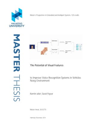
Chart 1 shows the performance of the decision fusion in presence of 1200 rpm engine
noise with 3.5 dB signal to noise ratio (SNR). Light blue bars indicate noise-free audio
results and red bars are the output of same system when the noisy signal fed. The
dramatic effect of the noise can be seen on digit “4” that drops to below 10 percent
when the noise introduced to it.
Chart 1 – Engine noise at 1200 rpm SNR 3.5 dB
The output of the visual system is presented with yellow bars they are steady in all
different noise scenarios. And finally dark blue bars show the fused result and final
output of the system. In most cases these results are above the video-only and always
0
10
20
30
40
50
60
70
80
90
100
digit 0 digit 1 digit 2 digit 3 digit 4 digit 5 digit 6 digit 7 digit 8 digit 9
noise-free audio
noisy audio
visual-only
fused
weighting %
SNR
Audio Video
noise free 78% 22%
15 % - 15 dB 65% 35%
25 % - 9.5 dB 55% 45%
40 % - 3.5 dB 30% 70%
42. The Potential of Visual Features to Improve Voice Recognition Systems
in Vehicles Noisy Environment
32
are better than noisy audio results that prove decision fusion method performs
efficiently.
Charts 2 to 4 show the overall performance of the system in different noise scenarios.
As describe before the average performance of the visual system remains steady
while performance of the audio systems drops increasingly by level of noise. Final
fused overall results are always above both of audio and visual systems.
Chart 2 - Engine noise at 600 rpm
Chart 3 - Engine noise at 1200 rpm
Chart 4 - Engine noise at 2000 rpm
43. Chapter 5. Experimental results33
For the comparison the results of audio-only systems vs. the fused results for
different noise levels are presented at Table 6. For the higher signal to noise ratios
there is ~7-10 percent improvement over the audio-only system and as the ratio of
the noise grows the amount of improvement is more significant (~15-25%).
Table 6 – left: engine noise at 600 rpm, right: engine noise at 1200 rpm,
down: engine noise at 2000 rpm
digits
SNR
Audio only Fused
noise free 87,32 90,71
15 % - 15 dB 78,93 86,38
25 % - 9.5 dB 67,41 80,49
40 % - 3.5 dB 49,15 70,27
digits
SNR
Audio only Fused
noise free 87,32 90,71
15 % - 15 dB 65,71 77,95
25 % - 9.5 dB 47,67 67,99
40 % - 3.5 dB 27,59 61,21
digits
SNR
Audio only Fused
noise free 87,32 90,71
15 % - 15 dB 52,95 68,66
25 % - 9.5 dB 33,79 57,90
40 % - 3.5 dB 16,96 59,15
44. The Potential of Visual Features to Improve Voice Recognition Systems
in Vehicles Noisy Environment
34
Figure 15 shows the results of fusion system for digit “2” from person 264 session 1
shot 1, for the noise-free scenario audio-only digit recognition works fine but when
the noise of 800 rpm with ratio of 75% added, audio-only system gives the wrong
result.
Figure 15 - Output results of digit 2 from person 264 session 1 shot 1, Left: using of 45
classifiers, Right: using top three most probable digits (three classifiers). Top first shows
picture noise-free audio output, second noisy audio results (75% with 800 rpm), third visual
output and the last one output of the fused results.
45. Chapter 5. Experimental results35
Since visual system works unaffected by noise final fused result are correct. The
fused results are a weighted sum combination of 30 percent audio-only system
output plus 70 percent visual prediction system.
Figure 16 - Output results of digit 4 from person 264 session 1 shot 1, Left: using of 45
classifiers, Right: using top four most probable digits (six classifiers). Top first shows picture
noise-free audio output, second noisy audio results (75% with 800 rpm), third visual output
and the last one output of the fused results.
Figure 16 illustrates the result of applying one more level of classification using four
most probable output digit of the system. Using 6 SVM classifier instead of 45, for
the noisy audio-only system both configurations fails to recognize correct output but
the fused results of the second system produces the correct result because most of the
SVM classifiers that are responsible for generating false results are removed in this
configuration.
46. The Potential of Visual Features to Improve Voice Recognition Systems
in Vehicles Noisy Environment
36
47. Chapter 6. Conclusion37
Chapter 6
6 Conclusion
6.1 Summary
Audio-visual systems are still subject of research, in the past three decades different
studies showed the potential of these systems not only for speech recognition but
also for the person verification and identification tasks. Unlike the audio-only speech
recognition which has been extensively studied and there is industry standards for
feature extraction and classification steps already in use in commercial applications,
for the video sequence processing different methods have been proposed for the
feature extraction yielding mixed results and still there is no commercial application
available relying on visual features or even audio-visual features in the real world.
Optical flow features used in this study shows promising potential for extracting
meaningful but small enough feature vectors for speech recognition. Isaac Faraj’s
works [31] on studying lip motion and his assumptions for feature reduction proves
to be good approach for visual feature extraction. Optical flow features eliminate the
need for precise lip contour tracking which by itself means less computational
demand on the system and it also helps with overall robustness of the system.
The experimental tests were performed on XM2VTS audio-visual database, since this
database is gathered for the person verification and identification tasks. However, it
is not designed with visual-speech recognition purposes in mind. This fact affects the
final results since the semi-automatically segmented digits in some cases lacked
enough illustrative information, useful for visual feature extraction. Overall for the
noise free audio-only environment we achieved 88% for average of all digits while
for the video-only because of the described issues it is about 62%. Final fused output
of the system is about 91% that shows decision fusion that chosen for combining
audio and video systems performs superior to both of them.
For the different noise scenarios (engine noise from the truck cab recorded with
respect to the drivers position in different rpm from 600 up to 2000) overall
audio-only system performance drops sharply from 88% for the noise free
environment to 17% for most extreme noise scenario, but since visual features are not
affected by the engine noise the overall performance of the audio-visual system
remains at about 60%.
For the current configuration of the system final results can still be improved by fine
tuning optical flow extraction and using better classification methods. As mentioned
previously SVM classifiers lack the ability to model time domain information, which
is logically important for any speech recognition system. By attempting to add time
48. The Potential of Visual Features to Improve Voice Recognition Systems
in Vehicles Noisy Environment
38
domain to the SVM classifier or using other classifiers that can do the time domain
modeling, overall result can be expected to improve.
6.2 Discussion
This study is inspired by Maycel Isaac Faraj’s work [1] but with the focus of possible
application in the automotive industry. His work did not include the effect of noise
on voice recognition system and overall performance of proposed audio-visual
system using two stand-alone systems (one for audio and one for video). By
considering different noise scenarios the feature fusion method used by Faraj turned
out to be unfeasible for our application. To design the system that can be able to
adopt it to different noise levels, decision fusion method has been selected by us
since by having separate audio and visual speech recognition systems; we were able
to give different weights to individual decision scores based on the noise level.
Also this approach solves the problem of audio and video synchronization since they
are completely independent systems but running in parallel together. This approach
requires training two different sets of classifiers for audio and video features in
contrast with single classifier used by Isaac Faraj. Although computation by two
independent systems decreases memory efficiency and computational efficiency it
gave us the ability to adaptively deal with the noise as a practical side effect.
Another study that utilized optical flow features is real time speaker identification
system purposed by Dieckmann et al. [34] combines audio features with the
optical flow of the mouth region plus the static facial features. In this study they used
point motion optical flows as opposed to line motion optical flow used by us.
6.3 Future work
By experimenting with XM2VTS database, which includes the frontal view of
subjects, the overall concept of audio-visual system for the truck cab environment is
studied. The next logical steps is to gather a specific database from the truck cab by
considering the current camera configuration already in place and with more
complete dictionary of commands to further investigate this system. After recording
the new data base near real time system can be implemented. This system requires
face tracking algorithm to be utilized (currently instead of having the face images
observed dynamically, we used pre-recorded data and “tracked” all video sequences
by semi automatically cropping frames extracting mouth regions (from each frame).
Since natural language processing (NLP) is state of art trend in speech recognition
community it is important to consider the possibility of adding this functionality to
the system. The output of voice recognition layer can be fed to NLP system to add
further capabilities to the system.
Audio and video features extracted can also be utilized for person identification and
verification tasks. Combining visual features will greatly increase anti spoofing
and liveness detection of audio-only identification and recognition systems.
49. Chapter 6. Conclusion39
There are numerous studies, including Isaac Faraj’s work, proving capabilities of the
multi-modal systems in person authentication field. However, the advantage of
video combined with lip-movements is that solves liveness, continuous person
authentication at the same time, without that the hand of the driver leaves the
driving wheel.
With the emergence of powerful smart phones and mobile devices equipped with
front facing camera, it is possible to run real time image processing in such devices.
On the other hand, the mobile nature of these devices poses challenges to any
application, which relies on extracting visual feature from the face of operator. Since
there is no fixed way to handle the device any feature extraction method should be
rotation, transition and scale invariant. Optical flow features can be good candidate
for this kind of applications including audio-visual speech recognition and person
identification and recognition.
In human-to-human communication optical flow features can be utilized to
reconstruct the avatar of the speaker in the receiving side of the system. Extracting
facial movements using the optical flow and transferring them over the line instead of
live video the speaker greatly reduces the bandwidth usage and opens up for new
applications for such systems. Since the human perception system uses the
combination of speakers lip movement in conjunction with hearing system, playing
the avatar of the speaker in the receiving side can also help with dealing the noise in
the environment.
Optical flow features also used in visual odometry systems, which can be, used as
additional sensor in the cars navigation systems in the environments like tunnels
which traditional systems are blocked. In active safety functions optical flow can be
used to detect moving objects in the environment along with their direction and
speed of movement such as pedestrians, animals etc.
50. The Potential of Visual Features to Improve Voice Recognition Systems
in Vehicles Noisy Environment
40
51. Chapter 6. Conclusion41
Bibliography
[1] Maycel Isaac Faraj.
Lip-motion biometrics for audio-visual identity recognition. Doctoral Thesis,
Chalmers Univ, 2008. ISSN 0346-718X.
[2] P. Jourlin, J. Luettin, D. Genoud, and H. Wassner.
Acoustic-labial speaker verification. Proceedings of the First International
Conference on Audio- and Video-Based Biometric Person Authentication, LNCS
1206, 1206:319–326, 1997. Lecture notes on Computer Science, ISBN:3- 540-
62660-3.
[3] J. Kittler, Y. Li, J. Matas, and M.U.R. Sanchez.
Combining evidence in multimodal personal identity recognition systems.
Proceedings of the First International Conference on Audio- and Video-Based
BiometricPerson Authentication, LNCS 1206, 1206:301–310, 1997. Lecture notes
on Computer Science, ISBN:3-540-62660-3.
[4] L. Liang, X. Liu, Y. Zhao, X. Pi, and A.V. Nefian.
Speaker independent audio–visual continuous speech recognition. IEEE
International Conference on Multimedia and Expo, 2002. ICME ’02. Proceedings.
2002, 2:26–29, 2002.
[5] X. Zhang, C.C. Broun, R.M. Mersereau, and M.A. Clements.
Automatic speechreading with applications to human-computer interfaces.
EURASIP Journal on Applied Signal Processing, 2002(11):1128–1247, 2002.
[6] McGurk, H & MacDonald, J.
"Hearing lips and seeing voices." Nature 264(5588) (1976): 746–748.
[7] J. Luettin, N.A. Thacker, and S.W. Beet.
Speaker identification by lipreading. Proceedings of the 4th International
Conference on Spoken Language Processing ICSLP0 96, pages 62–65, 1996.
[8] B.K.P. Horn and B.G. Schunck.
Determining optical flow. The journal of Artificial Intelligence, 17(1):185–203,
1981.
[9] B.D. Lucas and T. Kanade.
An iterative image registration technique with an application to stereo vision. In
Proc. of the seventh Int. Joint Conf. on Artificial Intelligence, Vancouver, pages 674–
679, 1981.
[10] M. A. Anusuya, S. K. Katti.
52. The Potential of Visual Features to Improve Voice Recognition Systems
in Vehicles Noisy Environment
42
Speech Recognition by Machine: A Review. International Journal of Computer
Science and Information Security, Vol. 6, No. 3, 2009
[11] S. Davis and P. Mermelstein.
Comparison of parametric representations for monosyllabic word recognition in
continuously spoken sentences. IEEE Trans. on Acoustics, Speech, and Signal
Processing, 28(4):357– 366, 1980.
[12] Dereje Teferi and Josef Bigun.
Damascening video databases for evaluation of face tracking and recognition - the
dxm2vts database. Pattern Recognition Letters, 28(15):2143–2156, 2007.
[13] J. Bigun,
Vision with Direction: A Systematic Introduction to Image Processing and computer
Vision, 2006. ISBN-10: 3540273220
[14] J. Bigun, G.H. Granlund, and J.Wiklund.
Multidimensional orientation estimation with applications to texture analysis of
optical flow. IEEE-Trans Pattern Analysis and Machine Intelligence, 13(8):775–790,
1991.
[15] J. Bigun and G.H. Granlund.
Optimal orientation detection of linear symmetry. In First International Conference
on Computer Vision, ICCV. IEEE Computer Society, pages 433–438, 1987. Report
LiTH-ISY-I-0828, Computer Vision Laboratory, Link¨oping University, Sweden 1986;
Lic. Thesis, Chapter 4, Linkoeping studies in science and technol-ogy No. 85 1986
[16] Asa Ben-Hur, Jason Weston,
“A User’s Guide to Support Vector Machines”, Data Mining Techniques for the Life
Sciences, 2009.
[17] J. Weston and C. Watkins.
Multi-class support vector machines. Royal Holloway Technical Report CSD-TR-98-
04, 1998.
[18] C-C. Chang and C-J. Lin.
LIBSVM: a library for support vector machines, 2001. Software available at
http://www.csie.ntu.edu.tw/~cjlin/libsvm.
[19] Chih-Wei Hsu, Chih-Chung Chang, and Chih-Jen Lin,
A Practical Guide to Support Vector Classification, Department of Computer Science
National Taiwan University, Taipei 106, Taiwan, April 15, 2010
[20] C. Sanderson Sanderson and K.K. Paliwal.
Identity verification using speech and face information. Digital Signal Processing,
14(5):449–480, 2004.
53. Chapter 6. Conclusion43
[21] P.S. Aleksic and A.K. Katsaggelos.
Audio-visual biometrics. Proceedings of the IEEE, 94(11):2025–2044, Nov. 2006.
[22] N.A. Fox, R. Gross, J.F. Cohn, and R.B. Reilly.
Robust biometric person identification using automatic classifier fusion of speech,
mouth, and face experts. Multimedia, IEEE Transactions on, 9(4):701–714, June 2007.
[23] K.R. Brunelli and D. Falavigna.
Person identification using multi- ple cues. IEEE Trans. on Pattern Analysis and
Machine Intelligence, 17(10):955–966, 1995.
[24] T.J. Wark, S. Sridharan, and V. Chandran.
Robust speaker verification via fusion of speech and lip modalities. IEEE
International Conference on Acoustics, Speech and Signal Processing 1999. ICASSP
99, 6:3061– 3064, 1999. ISBN: 0-7803-5041-3.
[25] J. Luettin and N.A. Thacker.
Speechreading using probabilistic models. Computer Vision and Image
Understanding, 65(2):163–178, 1997.
[26] C.C. Chibelushi, F. Deravi, and J.S.D. Mason.
A review of speech-based bimodal recognition. IEEE Trans. on Multimedia, 4(1):23–
37, 2002.
[27] K. Messer, J. Matas, J. Kittler, J. Luettin, and G. Maitre.
XM2VTSDB: The extended m2vts database. In Audio and Video based Person Au -
thentication - AVBPA99, pages 72–77. University of Maryland, 1999.
[28] Donald A.
Graft’s “Smart Deinterlacer Filter”, version 2.7,
url: ”http://neuron2.net/smart/smart.html” 2011
[29] “http://audacity.sourceforge.net/?lang=sv” 2011
[30] “http://www.ee.ic.ac.uk/hp/staff/dmb/voicebox/voicebox.html“ 2011
[31] Maycel Isaac Faraj and Josef Bigun.
Audio-visual person authentication using lip-motion from orientation maps. Pattern
Recognition Letters, 18(11): 1368–1382, 2007.
[32] Stefan M. Karlsson, Josef Bigün:
Lip-motion events analysis and lip segmentation using optical flow. Cvpr workshop
on biometrics, 138-145
[33] F. Provost.
Learning with imbalanced data sets 101. In AAAI 2000 workshop on imbalanced
data sets, 2000.
54. The Potential of Visual Features to Improve Voice Recognition Systems
in Vehicles Noisy Environment
44
[34] U. Dieckmann, P. Plankensteiner, and T. Wagner. Sesam:
A biometric person identification system using sensor fusion. Proceedings of the
First International Conference on Audio- and Video-Based Biometric Person
Authentication, LNCS 1206, 1206:301–310, 1997. Lecture notes on Computer Science,
ISBN:3-540-62660-3.
55. Chapter 6. Conclusion45
List of Abbreviations
BCC – Brightness Constancy Constrain
FAR – False Acceptance Rate
FRR – False Rejection Rate
LDA – Linear Discriminate Analysis
LES – Least-Squares Error
MFCC – Mel-Frequency Cepstral Coefficients
NLP – Natural Language Processing
PCA – Principal Component Analysis
RBF – Radial Basis Function
RPM – Revolutions Per Minute
SNR – Signal-to-Noise Ratio
SVM – Support Vector Machine
56. The Potential of Visual Features to Improve Voice Recognition Systems
in Vehicles Noisy Environment
46
60. PO Box 823, SE-301 18 Halmstad
Phone: +35 46 16 71 00
E-mail: registrator@hh.se
www.hh.se
Ramtin Jafari
Phone: +46 (0)72 2525792
eMail: ramtin.jafari@gmail.com
Master?s student in Embedded and
Intelligent Systems, Halmstad
University, Sweden
Bachelor?s degree in Computer
Engineering ? Hardware, Azad
University of Qazvin, Iran.
Area of Interest: Imag
Saeid Payvar
Phone: +46 (0)73 5631991
eMail: payvar@gmail.com
Master?s student in Embedded and
Intelligent Systems, Halmstad
University, Sweden
Bachelor?s degree in Software
Engineering, Azad University of
Shabstar, Iran.
Area of Interest: Image Processing,
Act
RamtinJafari
Phone: +46 (0)72 2525792
eMail: ramtin.jafari® gmail.com
Master's student inEmbedded andIntelligent Systems, HalmstadUniversity,Sweden
Bachelor'sdegree in Computer Engineering-Hardware,Azad University of Qazvin,Iran.
Area of Interest ImageProcessing,Active Safety, SignalProcessing,Embedded Systems.
Saeid Payvar
Phone: +46 (0)73 5631991
eMail: pawar@gmail.com
Master's student inEmbedded and Intelligent Systems, Halmstad University, Sweden
Bachelor's degree inSoftware Engineering, Azad University ofShabstar, Iran.
Area of Interest:Imafge Processing, Active Safety, Embedded Systems, Signal Processing.