Vector time series sas-writing sample

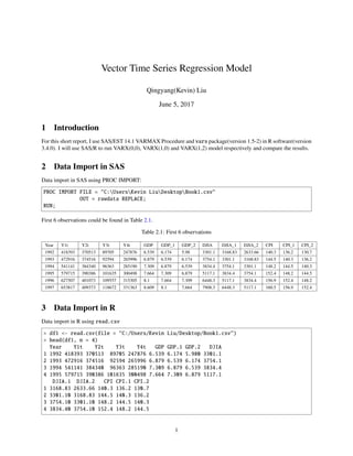
1. Vector Time Series Regression Model
Qingyang(Kevin) Liu
June 5, 2017
1 Introduction
For this short report, I use SAS/EST 14.1 VARMAX Procedure and vars package(version 1.5-2) in R software(version
3.4.0). I will use SAS/R to run VARX(0,0), VARX(1,0) and VARX(1,2) model respectively and compare the results.
2 Data Import in SAS
Data import in SAS using PROC IMPORT:
PROC IMPORT FILE = "C:UsersKevin LiuDesktopBook1.csv"
OUT = rawdata REPLACE;
RUN;
First 6 observations could be found in Table 2.1.
Table 2.1: First 6 observations
Year Y1t Y2t Y3t Y4t GDP GDP_1 GDP_2 DJIA DJIA_1 DJIA_2 CPI CPI_1 CPI_2
1992 418393 370513 89705 247876 6.539 6.174 5.98 3301.1 3168.83 2633.66 140.3 136.2 130.7
1993 472916 374516 92594 265996 6.879 6.539 6.174 3754.1 3301.1 3168.83 144.5 140.3 136.2
1994 541141 384340 96363 285190 7.309 6.879 6.539 3834.4 3754.1 3301.1 148.2 144.5 140.3
1995 579715 390386 101635 300498 7.664 7.309 6.879 5117.1 3834.4 3754.1 152.4 148.2 144.5
1996 627507 401073 109557 315305 8.1 7.664 7.309 6448.3 5117.1 3834.4 156.9 152.4 148.2
1997 653817 409373 118672 331363 8.609 8.1 7.664 7908.3 6448.3 5117.1 160.5 156.9 152.4
3 Data Import in R
Data import in R using read.csv
> df1 <- read.csv(file = "C:/Users/Kevin Liu/Desktop/Book1.csv")
> head(df1, n = 4)
Year Y1t Y2t Y3t Y4t GDP GDP.1 GDP.2 DJIA
1 1992 418393 370513 89705 247876 6.539 6.174 5.980 3301.1
2 1993 472916 374516 92594 265996 6.879 6.539 6.174 3754.1
3 1994 541141 384340 96363 285190 7.309 6.879 6.539 3834.4
4 1995 579715 390386 101635 300498 7.664 7.309 6.879 5117.1
DJIA.1 DJIA.2 CPI CPI.1 CPI.2
1 3168.83 2633.66 140.3 136.2 130.7
2 3301.10 3168.83 144.5 140.3 136.2
3 3754.10 3301.10 148.2 144.5 140.3
4 3834.40 3754.10 152.4 148.2 144.5
1

2. 4 VARX(0,0) by SAS and R
Table 4.1: Parameter Estimates - Least Square Estimations - SAS
Model Parameter Estimates
Equation Parameter Estimate Standard Error t Value Pr > |t| Variable
Y1t CONST1 777627.09661 467638.35696 1.66 0.1137 1
XL0_1_1 175401.30692 61484.95613 2.85 0.0106 GDP(t)
XL0_1_2 −36455.81505 84872.27913 −0.43 0.6726 GDP_1(t)
XL0_1_3 −75015.94665 56715.79355 −1.32 0.2025 GDP_2(t)
XL0_1_4 23.90672 7.96739 3.00 0.0077 DJIA_1(t)
XL0_1_5 −5779.45128 5541.26942 −1.04 0.3108 CPI(t)
Y2t CONST2 −27084.66345 127589.23833 −0.21 0.8343 1
XL0_2_1 4173.49774 16775.39621 0.25 0.8063 GDP(t)
XL0_2_2 −7546.18536 23156.33286 −0.33 0.7483 GDP_1(t)
XL0_2_3 7829.34724 15474.19024 0.51 0.6190 GDP_2(t)
XL0_2_4 1.24754 2.17380 0.57 0.5731 DJIA_1(t)
XL0_2_5 2466.32077 1511.86560 1.63 0.1202 CPI(t)
Y3t CONST3 −5201.66297 39518.52739 −0.13 0.8967 1
XL0_3_1 13974.91428 5195.88457 2.69 0.0150 GDP(t)
XL0_3_2 −4211.72612 7172.26771 −0.59 0.5643 GDP_1(t)
XL0_3_3 14931.18678 4792.85886 3.12 0.0060 GDP_2(t)
XL0_3_4 −0.04283 0.67330 −0.06 0.9500 DJIA_1(t)
XL0_3_5 −451.61857 468.27384 −0.96 0.3476 CPI(t)
Y4t CONST4 −54006.48887 125220.44460 −0.43 0.6714 1
XL0_4_1 29242.49149 16463.94790 1.78 0.0926 GDP(t)
XL0_4_2 9150.61303 22726.41747 0.40 0.6920 GDP_1(t)
XL0_4_3 −2403.83767 15186.89983 −0.16 0.8760 GDP_2(t)
XL0_4_4 −1.86762 2.13344 −0.88 0.3929 DJIA_1(t)
XL0_4_5 619.55937 1483.79664 0.42 0.6812 CPI(t)
Code in SAS:
PROC VARMAX DATA = rawdata;
MODEL Y1t Y2t Y3t Y4t = GDP GDP_1 GDP_2 DJIA_1 CPI/ METHOD = LS;
RUN;
2

3. Table 4.2: Parameter Estimates - Least Square Estimations - R
> reg1 <- lm(cbind(df1$Y1t,df1$Y2t,df1$Y3t,df1$Y4t) ~ df1$GDP +
+ df1$GDP.1 + df1$GDP.2 + df1$DJIA.1 + df1$CPI)
> reg1$coefficients
[,1] [,2] [,3] [,4]
(Intercept) 777627.09661 -27084.663452 -5201.6629663 -54006.488874
df1$GDP 175401.30692 4173.497742 13974.9142752 29242.491488
df1$GDP.1 -36455.81505 -7546.185360 -4211.7261226 9150.613030
df1$GDP.2 -75015.94665 7829.347243 14931.1867830 -2403.837672
df1$DJIA.1 23.90672 1.247541 -0.0428268 -1.867618
df1$CPI -5779.45128 2466.320767 -451.6185712 619.559370
In SAS VARMAX Procedure, we can choose to use least square estimation by adding METHOD = LS in MODEL clause.
lm in R software uses the method of least square estimation only. There is no significant difference between coefficients
in Table 4.1 and Table 4.2. Use summary(reg1), we can get standard error, t value and p-value just like Table 4.1.
However, the results from summary(reg1) is too lengthy so I decide to not to show.
According to Table 4.2 (round to 5 digits after decimal), the equation for VARX(0,0) model is


ˆy1,t
ˆy2,t
ˆy3,t
ˆy4,t


=


777627.09661
−27084.66345
−5201.66297
−54006.48887


+


175401.30692 −36455.81505 −75015.94665 23.90672 −5779.45128
4173.49774 −7546.18536 7829.34724 1.24754 2466.32077
13974.91428 −4211.72612 14931.18678 −0.04283 −451.61857
29242.49149 9150.61303 −2403.83767 −1.86762 619.55937




GDPt
GDPt−1
GDPt−2
DJIAt−1
CPIt


3

4. 5 VARX(1,0) by SAS and R
5.1 VARX(1,0) without restrictions
In R software, vars package provides VAR function to fit VARX model by least squares per equation. In SAS software,
we can chose ML, conditional ML or least squares. However, for this data, SAS software fails to estimate parameters
and shows ERROR: Optimization cannot be completed, if use ML or conditional ML.
Table 5.1: Model Parameter Estimations - SAS
Model Parameter Estimates
Equation Parameter Estimate Standard Error t Value Pr > |t| Variable
Y1t CONST1 −138568.2188 384566.44338 −0.36 0.7244 1
XL0_1_1 175712.21495 37440.58373 4.69 0.0004 GDP(t)
XL0_1_2 −238864.7623 72981.27416 −3.27 0.0061 GDP_1(t)
XL0_1_3 5206.34733 45878.71597 0.11 0.9114 GDP_2(t)
XL0_1_4 4.32965 9.07958 0.48 0.6414 DJIA_1(t)
XL0_1_5 −1838.52061 5367.62007 −0.34 0.7374 CPI(t)
AR1_1_1 0.78748 0.19798 3.98 0.0016 Y1t(t−1)
AR1_1_2 2.00610 1.26674 1.58 0.1373 Y2t(t−1)
AR1_1_3 −0.02937 2.00817 −0.01 0.9886 Y3t(t−1)
AR1_1_4 0.53449 2.47715 0.22 0.8325 Y4t(t−1)
Y2t CONST2 −90511.94320 42928.71297 −2.11 0.0550 1
XL0_2_1 5626.81231 4179.44961 1.35 0.2012 GDP(t)
XL0_2_2 23142.83745 8146.81630 2.84 0.0139 GDP_1(t)
XL0_2_3 −1960.13723 5121.38868 −0.38 0.7081 GDP_2(t)
XL0_2_4 −0.52221 1.01354 −0.52 0.6150 DJIA_1(t)
XL0_2_5 2649.37949 599.18130 4.42 0.0007 CPI(t)
AR1_2_1 0.00115 0.02210 0.05 0.9594 Y1t(t−1)
AR1_2_2 0.29378 0.14141 2.08 0.0581 Y2t(t−1)
AR1_2_3 0.53691 0.22417 2.40 0.0324 Y3t(t−1)
AR1_2_4 −1.00662 0.27652 −3.64 0.0030 Y4t(t−1)
Y3t CONST3 1950.28068 36837.27329 0.05 0.9586 1
XL0_3_1 4332.87985 3586.39980 1.21 0.2485 GDP(t)
XL0_3_2 1454.17407 6990.81053 0.21 0.8384 GDP_1(t)
XL0_3_3 8999.78992 4394.68089 2.05 0.0613 GDP_2(t)
XL0_3_4 0.04481 0.86973 0.05 0.9597 DJIA_1(t)
XL0_3_5 155.90712 514.15949 0.30 0.7665 CPI(t)
AR1_3_1 0.02446 0.01896 1.29 0.2196 Y1t(t−1)
AR1_3_2 −0.14084 0.12134 −1.16 0.2666 Y2t(t−1)
AR1_3_3 0.88377 0.19236 4.59 0.0005 Y3t(t−1)
AR1_3_4 −0.25965 0.23728 −1.09 0.2937 Y4t(t−1)
Y4t CONST4 66724.03690 32404.01465 2.06 0.0601 1
XL0_4_1 16288.90163 3154.78702 5.16 0.0002 GDP(t)
XL0_4_2 −10826.97884 6149.48682 −1.76 0.1018 GDP_1(t)
4

5. Table 5.1: Model Parameter Estimations - SAS
Model Parameter Estimates
Equation Parameter Estimate Standard Error t Value Pr > |t| Variable
XL0_4_3 −6046.35443 3865.79383 −1.56 0.1418 GDP_2(t)
XL0_4_4 1.28271 0.76506 1.68 0.1175 DJIA_1(t)
XL0_4_5 580.21030 452.28189 1.28 0.2219 CPI(t)
AR1_4_1 −0.01138 0.01668 −0.68 0.5071 Y1t(t−1)
AR1_4_2 −0.39193 0.10674 −3.67 0.0028 Y2t(t−1)
AR1_4_3 0.48076 0.16921 2.84 0.0139 Y3t(t−1)
AR1_4_4 0.86201 0.20873 4.13 0.0012 Y4t(t−1)
Table 5.2: Covariance matrix of residuals - SAS
Covariances of Innovations
Variable Y1t Y2t Y3t Y4t
Y1t 747331773.51 19587262.285 30483755.224 27425710.675
Y2t 19587262.285 9312502.7109 1240027.6894 2258369.7439
Y3t 30483755.224 1240027.6894 6857181.2306 1106124.7065
Y4t 27425710.675 2258369.7439 1106124.7065 5306013.0675
Table 5.3: Information Criteria of VARX(1,0) Model without restriction - SAS
Information Criteria
AICC 1502.229
HQC 1698.651
AIC 1684.372
SBC 1741.147
FPEC 6.278E29
Code in SAS:
PROC VARMAX DATA = rawdata;
MODEL Y1t Y2t Y3t Y4t = GDP GDP_1 GDP_2 DJIA_1 CPI/
P = 1 XLAG = 0 METHOD = LS;
RUN;
5

6. Table 5.4: Model Parameter Estimations - R
> library(vars)
> endogenous <- cbind.data.frame(df1$Y1t,df1$Y2t,df1$Y3t,df1$Y4t)
> names(endogenous) <- c("Y1t","Y2t","Y3t","Y4t")
> exogenous <- cbind.data.frame(df1$GDP,df1$GDP.1,
+ df1$GDP.2,df1$DJIA.1,df1$CPI)
> names(exogenous) <- c("GDP","GDP.1","GDP.2","DJIA.1","CPI")
> vars1 <- vars::VAR(y = endogenous, p = 1, type = "const", exogen = exogenous)
> summary(vars1)
VAR Estimation Results:
=========================
Endogenous variables: Y1t, Y2t, Y3t, Y4t
Deterministic variables: const
Sample size: 23
Log Likelihood: -876.728
Roots of the characteristic polynomial:
1.211 1.006 0.3468 0.3468
Call:
vars::VAR(y = endogenous, p = 1, type = "const", exogen = exogenous)
Estimation results for equation Y1t:
====================================
Y1t = Y1t.l1 + Y2t.l1 + Y3t.l1 + Y4t.l1 + const + GDP + GDP.1 + GDP.2 + DJIA.1 + CPI
Estimate Std. Error t value Pr(>|t|)
Y1t.l1 7.875e-01 1.980e-01 3.978 0.00158 **
Y2t.l1 2.006e+00 1.267e+00 1.584 0.13728
Y3t.l1 -2.937e-02 2.008e+00 -0.015 0.98855
Y4t.l1 5.345e-01 2.477e+00 0.216 0.83252
const -1.386e+05 3.846e+05 -0.360 0.72439
GDP 1.757e+05 3.744e+04 4.693 0.00042 ***
GDP.1 -2.389e+05 7.298e+04 -3.273 0.00605 **
GDP.2 5.206e+03 4.588e+04 0.113 0.91138
DJIA.1 4.330e+00 9.080e+00 0.477 0.64138
CPI -1.839e+03 5.368e+03 -0.343 0.73743
---
Signif. codes: 0 *** 0.001 ** 0.01 * 0.05 . 0.1 1
Residual standard error: 27340 on 13 degrees of freedom
Multiple R-Squared: 0.981, Adjusted R-squared: 0.9678
F-statistic: 74.39 on 9 and 13 DF, p-value: 1.036e-09
Estimation results for equation Y2t:
====================================
Y2t = Y1t.l1 + Y2t.l1 + Y3t.l1 + Y4t.l1 + const + GDP + GDP.1 + GDP.2 + DJIA.1 + CPI
Estimate Std. Error t value Pr(>|t|)
Y1t.l1 1.148e-03 2.210e-02 0.052 0.95938
Y2t.l1 2.938e-01 1.414e-01 2.078 0.05813 .
Y3t.l1 5.369e-01 2.242e-01 2.395 0.03238 *
Y4t.l1 -1.007e+00 2.765e-01 -3.640 0.00299 **
const -9.051e+04 4.293e+04 -2.108 0.05497 .
GDP 5.627e+03 4.179e+03 1.346 0.20121
6

7. GDP.1 2.314e+04 8.147e+03 2.841 0.01390 *
GDP.2 -1.960e+03 5.121e+03 -0.383 0.70810
DJIA.1 -5.222e-01 1.014e+00 -0.515 0.61504
CPI 2.649e+03 5.992e+02 4.422 0.00069 ***
---
Signif. codes: 0 *** 0.001 ** 0.01 * 0.05 . 0.1 1
Residual standard error: 3052 on 13 degrees of freedom
Multiple R-Squared: 0.9994, Adjusted R-squared: 0.999
F-statistic: 2453 on 9 and 13 DF, p-value: < 2.2e-16
Estimation results for equation Y3t:
====================================
Y3t = Y1t.l1 + Y2t.l1 + Y3t.l1 + Y4t.l1 + const + GDP + GDP.1 + GDP.2 + DJIA.1 + CPI
Estimate Std. Error t value Pr(>|t|)
Y1t.l1 2.446e-02 1.896e-02 1.290 0.219646
Y2t.l1 -1.408e-01 1.213e-01 -1.161 0.266627
Y3t.l1 8.838e-01 1.924e-01 4.594 0.000503 ***
Y4t.l1 -2.596e-01 2.373e-01 -1.094 0.293696
const 1.950e+03 3.684e+04 0.053 0.958582
GDP 4.333e+03 3.586e+03 1.208 0.248512
GDP.1 1.454e+03 6.991e+03 0.208 0.838443
GDP.2 9.000e+03 4.395e+03 2.048 0.061330 .
DJIA.1 4.481e-02 8.697e-01 0.052 0.959696
CPI 1.559e+02 5.142e+02 0.303 0.766515
---
Signif. codes: 0 *** 0.001 ** 0.01 * 0.05 . 0.1 1
Residual standard error: 2619 on 13 degrees of freedom
Multiple R-Squared: 0.9992, Adjusted R-squared: 0.9986
F-statistic: 1774 on 9 and 13 DF, p-value: < 2.2e-16
Estimation results for equation Y4t:
====================================
Y4t = Y1t.l1 + Y2t.l1 + Y3t.l1 + Y4t.l1 + const + GDP + GDP.1 + GDP.2 + DJIA.1 + CPI
Estimate Std. Error t value Pr(>|t|)
Y1t.l1 -1.138e-02 1.668e-02 -0.682 0.507136
Y2t.l1 -3.919e-01 1.067e-01 -3.672 0.002817 **
Y3t.l1 4.808e-01 1.692e-01 2.841 0.013890 *
Y4t.l1 8.620e-01 2.087e-01 4.130 0.001185 **
const 6.672e+04 3.240e+04 2.059 0.060099 .
GDP 1.629e+04 3.155e+03 5.163 0.000182 ***
GDP.1 -1.083e+04 6.149e+03 -1.761 0.101790
GDP.2 -6.046e+03 3.866e+03 -1.564 0.141810
DJIA.1 1.283e+00 7.651e-01 1.677 0.117484
CPI 5.802e+02 4.523e+02 1.283 0.221945
---
Signif. codes: 0 *** 0.001 ** 0.01 * 0.05 . 0.1 1
Residual standard error: 2303 on 13 degrees of freedom
Multiple R-Squared: 0.9998, Adjusted R-squared: 0.9997
F-statistic: 8559 on 9 and 13 DF, p-value: < 2.2e-16
7

8. Covariance matrix of residuals:
Y1t Y2t Y3t Y4t
Y1t 747331774 19587262 30483755 27425711
Y2t 19587262 9312503 1240028 2258370
Y3t 30483755 1240028 6857181 1106125
Y4t 27425711 2258370 1106125 5306013
Correlation matrix of residuals:
Y1t Y2t Y3t Y4t
Y1t 1.0000 0.2348 0.4258 0.4355
Y2t 0.2348 1.0000 0.1552 0.3213
Y3t 0.4258 0.1552 1.0000 0.1834
Y4t 0.4355 0.3213 0.1834 1.0000
There is no significant difference between (Table 5.1& Table 5.2) and Table 5.4. SAS and R software will give same
results. According to either (Table 5.1& Table 5.2) or Table 5.4, the equation of VARX(1,0) model (round to 4 digits
after decimal) is:


y1,t
y2,t
y3,t
y4,t


=


−138568.2188
−90511.9432
1950.2807
66724.0369


+


0.7875 2.0061 −0.0294 0.5345
0.0012 0.2938 0.5369 −1.0066
0.0245 −0.1408 0.8838 −0.2597
−0.0114 −0.3919 0.4808 0.8620




y1,t−1
y2,t−1
y3,t−1
y4,t−1


+


175712.2150 −238864.7623 5206.3473 4.3297 −1838.5206
5626.8123 23142.8375 −1960.1372 −0.5222 2649.3795
4332.8799 1454.1741 8999.7899 0.0448 155.9071
16288.9016 −10826.9788 −6046.3544 1.2827 580.2103




GDPt
GDPt−1
GDPt−2
DJIAt−1
CPIt


+


ξ1,t
ξ2,t
ξ3,t
ξ4,t


where ξt is a 4-dimensional Gaussian vector white noise process, VWN(0, Σ).
ˆΣ =


747331773.5 19587262.29 30483755.22 27425710.68
19587262.29 9312502.711 1240027.689 2258369.744
30483755.22 1240027.689 6857181.231 1106124.707
27425710.68 2258369.744 1106124.707 5306013.068


8

9. 5.2 VARX(1,0) with restrictions
In SAS VARMAX Procedure, we can restrict certain parameters to zero by using RESTRICT clause. For example, if
we want to restrict parameter AR1_2_1 to 0 (due to small p-value), we can type AR(1,2,1) = 0 under RESTRICT
clause. Estimated parameters for VARX(1,0) model with restrictions can be found in Table 5.5. The list of restricted
parameters can be found in Table 5.6. Comparing Table 5.3 and Table 5.8, we have that restrictions are necessary,
since information criterion has became smaller after restrictions.
Table 5.5: Model Parameter Estimates with restriction - SAS
Model Parameter Estimates
Equation Parameter Estimate Standard Error t Value Pr > |t| Variable
Y1t CONST1 113286.36653 27644.23053 4.10 0.0013 1
XL0_1_1 148657.85049 23464.22394 6.34 0.0001 GDP(t)
XL0_1_2 −137991.3556 23158.02582 −5.96 0.0001 GDP_1(t)
XL0_1_3 0.00000 0.00000 GDP_2(t)
XL0_1_4 −0.00000 0.00000 −0.00 1.0000 DJIA_1(t)
XL0_1_5 0.00000 0.00000 CPI(t)
AR1_1_1 0.62660 0.05954 10.52 0.0001 Y1t(t−1)
AR1_1_2 0.00000 0.00000 Y2t(t−1)
AR1_1_3 0.00000 0.00000 0.00 1.0000 Y3t(t−1)
AR1_1_4 −0.00000 0.00000 Y4t(t−1)
Y2t CONST2 −72036.88292 28613.39230 −2.52 0.0257 1
XL0_2_1 0.00000 0.00000 GDP(t)
XL0_2_2 25823.80058 4572.82339 5.65 0.0001 GDP_1(t)
XL0_2_3 0.00000 0.00000 GDP_2(t)
XL0_2_4 0.00000 0.00000 DJIA_1(t)
XL0_2_5 2564.86960 355.01512 7.22 0.0001 CPI(t)
AR1_2_1 −0.00000 0.00000 Y1t(t−1)
AR1_2_2 0.26999 0.09165 2.95 0.0114 Y2t(t−1)
AR1_2_3 0.58993 0.17364 3.40 0.0048 Y3t(t−1)
AR1_2_4 −0.98403 0.14113 −6.97 0.0001 Y4t(t−1)
Y3t CONST3 0.00000 0.00043 0.00 1.0000 1
XL0_3_1 −0.00000 0.00004 −0.00 1.0000 GDP(t)
XL0_3_2 0.00000 0.00006 0.00 1.0000 GDP_1(t)
XL0_3_3 3237.36876 708.26849 4.57 0.0005 GDP_2(t)
XL0_3_4 −0.00000 0.00000 DJIA_1(t)
XL0_3_5 0.00000 0.00001 0.00 1.0000 CPI(t)
AR1_3_1 −0.00000 0.00000 Y1t(t−1)
AR1_3_2 0.00000 0.00000 Y2t(t−1)
AR1_3_3 0.85834 0.04162 20.63 0.0001 Y3t(t−1)
AR1_3_4 0.00000 0.00000 Y4t(t−1)
Y4t CONST4 140261.51485 10739.58436 13.06 0.0001 1
XL0_4_1 17217.97530 1606.13048 10.72 0.0001 GDP(t)
XL0_4_2 0.00000 0.00000 GDP_1(t)
9

10. Table 5.5: Model Parameter Estimates with restriction - SAS
Model Parameter Estimates
Equation Parameter Estimate Standard Error t Value Pr > |t| Variable
XL0_4_3 −0.00000 0.00004 −0.00 1.0000 GDP_2(t)
XL0_4_4 −0.00000 0.00000 DJIA_1(t)
XL0_4_5 −0.00000 0.00000 CPI(t)
AR1_4_1 0.00000 0.00000 Y1t(t−1)
AR1_4_2 −0.53386 0.03756 −14.21 0.0001 Y2t(t−1)
AR1_4_3 0.56381 0.11419 4.94 0.0003 Y3t(t−1)
AR1_4_4 0.62493 0.05436 11.50 0.0001 Y4t(t−1)
Table 5.6: List of Restricted Parameters - SAS
Testing of the Restricted Parameters
Parameter Estimate Standard Error t Value Pr > |t| Equation
Restrict0 0.00002 0.00004 0.62 0.5606 XL0_1_3 = 0
Restrict1 0.21751 0.23303 0.93 0.3866 XL0_1_4 = 0
Restrict2 −0.00050 0.00035 −1.45 0.1982 XL0_1_5 = 0
Restrict3 8.58161 2.16870 3.96 0.0075 AR1_1_2 = 0
Restrict4 0.32744 0.93543 0.35 0.7383 AR1_1_3 = 0
Restrict5 −4.83637 1.85136 −2.61 0.0400 AR1_1_4 = 0
Restrict6 0.00027 0.00031 0.90 0.4047 XL0_2_1 = 0
Restrict7 −0.00018 0.00027 −0.66 0.5310 XL0_2_3 = 0
Restrict8 −2.22345 1.96019 −1.13 0.2999 XL0_2_4 = 0
Restrict9 −47.29467 98.35604 −0.48 0.6477 AR1_2_1 = 0
Restrict10 0.00210 0.00078 2.71 0.0350 XL0_3_1 = 0
Restrict11 0.00114 0.00046 2.45 0.0495 XL0_3_2 = 0
Restrict12 16.54631 3.57244 4.63 0.0036 XL0_3_4 = 0
Restrict13 −0.01865 0.02149 −0.87 0.4188 XL0_3_5 = 0
Restrict14 778.31531 189.03532 4.12 0.0062 AR1_3_1 = 0
Restrict15 −94.79572 48.84643 −1.94 0.1003 AR1_3_2 = 0
Restrict16 31.55622 21.84122 1.44 0.1986 AR1_3_4 = 0
Restrict17 −0.00063 0.00023 −2.75 0.0331 XL0_4_2 = 0
Restrict18 −0.00074 0.00038 −1.94 0.1005 XL0_4_3 = 0
Restrict19 −0.11591 2.79868 −0.04 0.9683 XL0_4_4 = 0
Restrict20 0.01664 0.00374 4.45 0.0044 XL0_4_5 = 0
Restrict21 −274.38730 138.89380 −1.98 0.0956 AR1_4_1 = 0
Restrict22 −0.00019 0.00021 −0.87 0.4172 CONST3 = 0
10

11. Table 5.7: Covariance matrix of residuals - SAS
Covariances of Innovations
Variable Y1t Y2t Y3t Y4t
Y1t 1761675919.1 38609353.320 91676797.771 58144304.548
Y2t 38609353.320 12351414.075 2083268.8031 4733015.7931
Y3t 91676797.771 2083268.8031 23332387.275 104685.48563
Y4t 58144304.548 4733015.7931 104685.48563 14179433.415
Table 5.8: Information Criteria of VARX(1,0) Model with restrictions - SAS
Information Criteria
AICC 1412.039
HQC 1722.15
AIC 1714.439
SBC 1745.098
FPEC 1.714E31
Code in SAS:
PROC VARMAX DATA = rawdata;
MODEL Y1t Y2t Y3t Y4t = GDP GDP_1 GDP_2 DJIA_1 CPI/
P = 1 XLAG = 0 METHOD = LS;
RESTRICT XL(0,1,3) = 0, XL(0,1,4) = 0, XL(0,1,5) = 0,
AR(1,1,2) = 0, AR(1,1,3) = 0, AR(1,1,4) = 0,
XL(0,2,1) = 0, XL(0,2,3) = 0, XL(0,2,4) = 0,
AR(1,2,1) = 0, XL(0,3,1) = 0, XL(0,3,2) = 0,
XL(0,3,4) = 0, XL(0,3,5) = 0, AR(1,3,1) = 0,
AR(1,3,2) = 0, AR(1,3,4) = 0, XL(0,4,2) = 0,
XL(0,4,3) = 0, XL(0,4,4) = 0, XL(0,4,5) = 0,
AR(1,4,1) = 0, CONST(3) = 0;
RUN;
By adding same restriction as in Table 5.6,we have estimated parameters,shown in Table 5.9 , by R software.
The difference between Table 5.9 and Table 5.5 is large. So far, I have not figured out the reason causing the difference.
11

12. According to Table 5.5 and Table 5.7, the equation for VARX(1,0) with restrictions is


y1,t
y2,t
y3,t
y4,t


=


113286.3665
−72036.8829
0
140261.5149


+


0.6266 0 0 0
0 0.2700 0.5899 −0.9840
0 0 0.8583 0
0 −0.5339 0.5638 0.6249




y1,t−1
y2,t−1
y3,t−1
y4,t−1


+


148657.8505 −137991.3556 0 0 0
0 25823.8006 0 0 2564.8696
0 0 3237.3688 0 0
17217.9753 0 0 0 0




GDPt
GDPt−1
GDPt−2
DJIAt−1
CPIt


+


ξ1,t
ξ2,t
ξ3,t
ξ4,t


where ξt is a 4-dimensional Gaussian vector white noise process, VWN(0, Σ).
Σ =


1761675919.1 38609353.320 91676797.771 58144304.548
38609353.320 12351414.075 2083268.8031 4733015.7931
91676797.771 2083268.8031 23332387.275 104685.48563
58144304.548 4733015.7931 104685.48563 14179433.415


The vars::restrict function provides a another way to restrict parameters by set up a threshold value of t values. I
don’t want to make this report too lengthy, so I only put R code below. We can check the restrictions matrix after build
a VAR model by checking $restrictions.
vars3 <- vars::restrict(vars1, method = "ser", thresh = 1.98)
vars3
vars3$restrictions
According to Table 5.9, the equation for VARX(1,0) with restrictions is


y1,t
y2,t
y3,t
y4,t


=


73848.4928
−96564.0734
0
136710.6481


+


0.6903 0 0 0
0 0.2394 0.6076 −1.0659
0 0 0.8626 0
0 −0.5193 0.5713 0.5692




y1,t−1
y2,t−1
y3,t−1
y4,t−1


+


187845.6485 −179622.7019 0 0 0
0 26520.1714 0 0 2911.4930
0 0 3164.6544 0 0
18929.6708 0 0 0 0




GDPt
GDPt−1
GDPt−2
DJIAt−1
CPIt


+


ξ1,t
ξ2,t
ξ3,t
ξ4,t


where ξt is a 4-dimensional Gaussian vector white noise process, VWN(0, Σ).
ˆΣ =


1516005840 17195013 41775322 25952984
17195013 11553816 2117432 2171713
41775322 2117432 23324172 −1484581
25952984 2171713 −1484581 13165568


12

13. Table 5.9: Model Parameter Estimates with restriction - R
> vars1 <- vars::VAR(y = endogenous, p = 1, type = "const",
+ exogen = exogenous)
> matrix1 <- matrix( data = c(1,0,0,0,1,1,1,0,0,0,
+ 0,1,1,1,1,0,1,0,0,1,
+ 0,0,1,0,0,0,0,1,0,0,
+ 0,1,1,1,1,1,0,0,0,0),byrow = T,nrow = 4)
> vars2 <- vars::restrict(vars1, method = "manual", resmat = matrix1)
> options(scipen=999) ##remove scientific notation##
> summary(vars2)
VAR Estimation Results:
=========================
Endogenous variables: Y1t, Y2t, Y3t, Y4t
Deterministic variables: const
Sample size: 23
Log Likelihood: -916.197
Roots of the characteristic polynomial:
1.166 0.8626 0.6903 0.3578
Call:
vars::VAR(y = endogenous, p = 1, type = "const", exogen = exogenous)
Estimation results for equation Y1t:
====================================
Y1t = Y1t.l1 + const + GDP + GDP.1
Estimate Std. Error t value Pr(>|t|)
Y1t.l1 0.69031 0.08233 8.385 0.0000000828 ***
const 73848.49279 35077.34646 2.105 0.0488 *
GDP 187845.64848 31696.84668 5.926 0.0000105030 ***
GDP.1 -179622.70188 31212.50807 -5.755 0.0000151661 ***
---
Signif. codes: 0 *** 0.001 ** 0.01 * 0.05 . 0.1 1
Residual standard error: 32210 on 19 degrees of freedom
Multiple R-Squared: 0.9987, Adjusted R-squared: 0.9984
F-statistic: 3567 on 4 and 19 DF, p-value: < 0.00000000000000022
Estimation results for equation Y2t:
====================================
Y2t = Y2t.l1 + Y3t.l1 + Y4t.l1 + const + GDP.1 + CPI
Estimate Std. Error t value Pr(>|t|)
Y2t.l1 0.23938 0.09249 2.588 0.01914 *
Y3t.l1 0.60757 0.17404 3.491 0.00280 **
Y4t.l1 -1.06594 0.14254 -7.478 0.000000903 ***
const -96564.07343 29408.48025 -3.284 0.00438 **
GDP.1 26520.17136 4642.52701 5.712 0.000025408 ***
CPI 2911.49295 365.93154 7.956 0.000000393 ***
---
Signif. codes: 0 *** 0.001 ** 0.01 * 0.05 . 0.1 1
Residual standard error: 2972 on 17 degrees of freedom
13

14. Multiple R-Squared: 1, Adjusted R-squared: 1
F-statistic: 1.158e+05 on 6 and 17 DF, p-value: < 0.00000000000000022
Estimation results for equation Y3t:
====================================
Y3t = Y3t.l1 + GDP.2
Estimate Std. Error t value Pr(>|t|)
Y3t.l1 0.86262 0.06116 14.10 0.00000000000351 ***
GDP.2 3164.65437 1040.84561 3.04 0.00622 **
---
Signif. codes: 0 *** 0.001 ** 0.01 * 0.05 . 0.1 1
Residual standard error: 3800 on 21 degrees of freedom
Multiple R-Squared: 0.9997, Adjusted R-squared: 0.9997
F-statistic: 3.504e+04 on 2 and 21 DF, p-value: < 0.00000000000000022
Estimation results for equation Y4t:
====================================
Y4t = Y2t.l1 + Y3t.l1 + Y4t.l1 + const + GDP
Estimate Std. Error t value Pr(>|t|)
Y2t.l1 -0.51933 0.05457 -9.516 0.0000000190 ***
Y3t.l1 0.57126 0.16752 3.410 0.00312 **
Y4t.l1 0.56923 0.07831 7.269 0.0000009323 ***
const 136710.64808 15742.01611 8.684 0.0000000747 ***
GDP 18929.67077 2270.66803 8.337 0.0000001356 ***
---
Signif. codes: 0 *** 0.001 ** 0.01 * 0.05 . 0.1 1
Residual standard error: 3084 on 18 degrees of freedom
Multiple R-Squared: 1, Adjusted R-squared: 1
F-statistic: 1.23e+05 on 5 and 18 DF, p-value: < 0.00000000000000022
Covariance matrix of residuals:
Y1t Y2t Y3t Y4t
Y1t 1516005840 17195013 41775322 25952984
Y2t 17195013 11553816 2117432 2171713
Y3t 41775322 2117432 23324172 -1484581
Y4t 25952984 2171713 -1484581 13165568
Correlation matrix of residuals:
Y1t Y2t Y3t Y4t
Y1t 1.0000 0.1299 0.22216 0.18370
Y2t 0.1299 1.0000 0.12899 0.17608
Y3t 0.2222 0.1290 1.00000 -0.08472
Y4t 0.1837 0.1761 -0.08472 1.00000
14

15. 6 VARX(1,2) by SAS and R
6.1 VARX(1,2) without restriction
It is relatively easy to build VARX(1,2) in SAS VARMAX Procedure. We only need to set XLAG = 2 to build
VARX(1,2) model instead of VARX(1,0) model.
Table 6.1: Model Parameter Estimates - SAS
Model Parameter Estimates
Equation Parameter Estimate Standard Error t Value Pr > |t| Variable
Y1t CONST1 246291.33186 458196.58397 0.54 0.6055 1
XL0_1_1 146505.34650 60180.25031 2.43 0.0409 GDP(t)
XL0_1_2 14.73901 6.60985 2.23 0.0563 DJIA(t)
XL0_1_3 2900.88130 6561.59680 0.44 0.6701 CPI(t)
XL1_1_1 −206911.7800 82975.86467 −2.49 0.0373 GDP(t−1)
XL1_1_2 −4.24463 8.55150 −0.50 0.6330 DJIA(t−1)
XL1_1_3 −5151.50086 8282.69903 −0.62 0.5513 CPI(t−1)
XL2_1_1 12981.71826 76643.35322 0.17 0.8697 GDP(t−2)
XL2_1_2 9.35419 7.79523 1.20 0.2645 DJIA(t−2)
XL2_1_3 −1814.21638 7076.44976 −0.26 0.8041 CPI(t−2)
AR1_1_1 0.60066 0.16694 3.60 0.0070 Y1t(t−1)
AR1_1_2 1.76350 1.28400 1.37 0.2069 Y2t(t−1)
AR1_1_3 1.84361 2.07645 0.89 0.4005 Y3t(t−1)
AR1_1_4 −0.20759 2.17423 −0.10 0.9263 Y4t(t−1)
Y2t CONST2 20797.38838 62424.41781 0.33 0.7476 1
XL0_2_1 1130.01150 8198.91990 0.14 0.8938 GDP(t)
XL0_2_2 1.47731 0.90052 1.64 0.1395 DJIA(t)
XL0_2_3 4042.86691 893.94787 4.52 0.0019 CPI(t)
XL1_2_1 20853.15886 11304.58023 1.84 0.1023 GDP(t−1)
XL1_2_2 −1.19657 1.16505 −1.03 0.3344 DJIA(t−1)
XL1_2_3 −1394.33701 1128.42977 −1.24 0.2516 CPI(t−1)
XL2_2_1 14235.08848 10441.84281 1.36 0.2099 GDP(t−2)
XL2_2_2 −0.36410 1.06202 −0.34 0.7406 DJIA(t−2)
XL2_2_3 −1620.59745 964.09112 −1.68 0.1313 CPI(t−2)
AR1_2_1 0.00238 0.02274 0.10 0.9192 Y1t(t−1)
AR1_2_2 0.48832 0.17493 2.79 0.0235 Y2t(t−1)
AR1_2_3 0.88958 0.28289 3.14 0.0137 Y3t(t−1)
AR1_2_4 −1.19789 0.29622 −4.04 0.0037 Y4t(t−1)
Y3t CONST3 −16601.31475 62350.69440 −0.27 0.7968 1
XL0_3_1 5036.70168 8189.23695 0.62 0.5556 GDP(t)
XL0_3_2 0.08934 0.89946 0.10 0.9233 DJIA(t)
XL0_3_3 148.12889 892.89212 0.17 0.8724 CPI(t)
XL1_3_1 3848.29397 11291.22949 0.34 0.7420 GDP(t−1)
15

16. Table 6.1: Model Parameter Estimates - SAS
Model Parameter Estimates
Equation Parameter Estimate Standard Error t Value Pr > |t| Variable
XL1_3_2 −0.53123 1.16368 −0.46 0.6602 DJIA(t−1)
XL1_3_3 −786.20005 1127.09709 −0.70 0.5052 CPI(t−1)
XL2_3_1 2600.71516 10429.51096 0.25 0.8094 GDP(t−2)
XL2_3_2 1.13973 1.06076 1.07 0.3140 DJIA(t−2)
XL2_3_3 983.05865 962.95252 1.02 0.3372 CPI(t−2)
AR1_3_1 0.01275 0.02272 0.56 0.5901 Y1t(t−1)
AR1_3_2 −0.13102 0.17472 −0.75 0.4748 Y2t(t−1)
AR1_3_3 0.72754 0.28256 2.57 0.0329 Y3t(t−1)
AR1_3_4 −0.15187 0.29587 −0.51 0.6216 Y4t(t−1)
Y4t CONST4 51273.01509 58112.47272 0.88 0.4033 1
XL0_4_1 21142.74305 7632.58234 2.77 0.0243 GDP(t)
XL0_4_2 0.14013 0.83832 0.17 0.8714 DJIA(t)
XL0_4_3 1038.33164 832.19873 1.25 0.2474 CPI(t)
XL1_4_1 −16451.40806 10523.72026 −1.56 0.1566 GDP(t−1)
XL1_4_2 0.43431 1.08458 0.40 0.6993 DJIA(t−1)
XL1_4_3 −355.72054 1050.48387 −0.34 0.7436 CPI(t−1)
XL2_4_1 −2811.35435 9720.57612 −0.29 0.7798 GDP(t−2)
XL2_4_2 1.29428 0.98866 1.31 0.2268 DJIA(t−2)
XL2_4_3 18.65800 897.49686 0.02 0.9839 CPI(t−2)
AR1_4_1 −0.01905 0.02117 −0.90 0.3946 Y1t(t−1)
AR1_4_2 −0.39139 0.16285 −2.40 0.0429 Y2t(t−1)
AR1_4_3 0.36930 0.26335 1.40 0.1984 Y3t(t−1)
AR1_4_4 0.82453 0.27575 2.99 0.0173 Y4t(t−1)
Table 6.2: Covariance matrix of residuals - SAS
Covariances of Innovations
Variable Y1t Y2t Y3t Y4t
Y1t 424276632.59 25554671.664 16950478.870 25348523.889
Y2t 25554671.664 7875069.9583 3792478.1325 3855028.3952
Y3t 16950478.870 3792478.1325 7856479.9841 −43175.39097
Y4t 25348523.889 3855028.3952 −43175.39097 6824708.8697
Code in SAS:
PROC VARMAX DATA = rawdata;
MODEL Y1t Y2t Y3t Y4t = GDP DJIA CPI/
P = 1 XLAG = 2 METHOD = LS;
RUN;
16

17. Table 6.3: Information Criteria of VAR(1,2) model without restriction - SAS
Information Criteria
AICC 1392.215
HQC 1605.712
AIC 1588.749
SBC 1660.757
FPEC 4.294E29
There are several packages available in R to fit VARX models. However, packages like MTS, BigVAR and fastVAR all
use R base function solve with default tolerance level,1e-16. This is problematic for this dataset. If the tolerance level
is "high"(large numeric value), the software will treat input matrix as singular matrix computationally. Unfortunately,
I have not found any package that provides function to change the tolerance level. Later on, I will modify MTS:VARX
function by adding a component,tol, so we can estimate parameters of VAR(1,2) model.Error message from using
MTS::VARX is shown in Table 6.4, line7 and 8.
Table 6.4: Fail to Estimate VARX(1,2) by MTS::VARX - R
1 > library(MTS)
2 > endogenous <- cbind.data.frame(df1$Y1t,df1$Y2t,df1$Y3t,df1$Y4t)
3 > names(endogenous) <- c("Y1t","Y2t","Y3t","Y4t")
4 > exogenous <- cbind(df1$GDP,df1$DJIA,df1$CPI)
5 > names(exogenous) <- c("GDP","DJIA","CPI")
6 > MTS::VARX(zt = df1[,2:5], p = 1, xt = exogenous, m = 2, include.mean = T)
7 Error in solve.default(xpx) :
8 system is computationally singular: reciprocal condition number = 5.14308e-17
There isn’t significant difference between the estimated parameters from Table 6.1 and Table 6.5. R and SAS software
give same estimated parameters. However, the se / standard error and covariance matrix of residuals from R and SAS
output are different! The modified varx function can be found at section 6.2.
Table 6.5: Model Parameter Estimates - R
1 > exogenous <- cbind(df1$GDP,df1$DJIA,df1$CPI)
2 > names(exogenous) <- c("GDP","DJIA","CPI")
3 > varx(zt = df1[,2:5], p = 1, xt = exogenous, m = 2,
4 + include.mean = T, tol = 1e-17)
5 constant term:
6 est: 246291.3 20797.39 -16601.31 51273.02
7 se: 276302.9 37643.34 37598.88 35043.14
8 AR( 1 ) matrix
9 Y1t Y2t Y3t Y4t
10 Y1t 0.601 1.764 1.844 -0.208
11 Y2t 0.002 0.488 0.890 -1.198
12 Y3t 0.013 -0.131 0.728 -0.152
13 Y4t -0.019 -0.391 0.369 0.825
14 standard errors
15 [,1] [,2] [,3] [,4]
16 [1,] 0.101 0.774 1.252 1.311
17 [2,] 0.014 0.105 0.171 0.179
18 [3,] 0.014 0.105 0.170 0.178
17

18. 19 [4,] 0.013 0.098 0.159 0.166
20 Coefficients of exogenous
21 lag- 0 coefficient matrix
22
23 Y1t 146505.347 14.739 2900.881
24 Y2t 1130.012 1.477 4042.867
25 Y3t 5036.702 0.089 148.129
26 Y4t 21142.743 0.140 1038.332
27 standard errors
28 [,1] [,2] [,3]
29 [1,] 36290.056 3.986 3956.792
30 [2,] 4944.135 0.543 539.071
31 [3,] 4938.296 0.542 538.434
32 [4,] 4602.620 0.506 501.835
33 lag- 1 coefficient matrix
34
35 Y1t -206911.780 -4.245 -5151.501
36 Y2t 20853.159 -1.197 -1394.337
37 Y3t 3848.294 -0.531 -786.200
38 Y4t -16451.408 0.434 -355.721
39 standard errors
40 [,1] [,2] [,3]
41 [1,] 50036.329 5.157 4994.655
42 [2,] 6816.918 0.703 680.469
43 [3,] 6808.868 0.702 679.665
44 [4,] 6346.042 0.654 633.466
45 lag- 2 coefficient matrix
46
47 Y1t 12981.718 9.354 -1814.216
48 Y2t 14235.088 -0.364 -1620.597
49 Y3t 2600.715 1.140 983.059
50 Y4t -2811.354 1.294 18.658
51 standard errors
52 [,1] [,2] [,3]
53 [1,] 46217.681 4.701 4267.260
54 [2,] 6296.668 0.640 581.369
55 [3,] 6289.232 0.640 580.682
56 [4,] 5861.728 0.596 541.211
57 Residual Covariance Matrix
58 Y1t Y2t Y3t Y4t
59 Y1t 154282412 9292608 6163810.50 9217645.05
60 Y2t 9292608 2863662 1379082.96 1401828.51
61 Y3t 6163810 1379083 2856901.81 -15700.14
62 Y4t 9217645 1401829 -15700.14 2481712.32
63 ===========
64 Information criteria:
65 AIC: 67.30676
66 BIC: 70.08395
18

19. According to (Table 6.1& Table 6.2) or Table 6.5, the equation for VARX(1,2) is


y1,t
y2,t
y3,t
y4,t


=


246291.3319
20797.3884
−16601.3148
51273.0151


+


146505.3465 14.7390 2900.8813
1130.0115 1.4773 4042.8669
5036.7017 0.0893 148.1289
21142.7431 0.1401 1038.3316




GDPt
DJIAt
CPIt


+


−206911.7800 −4.2446 −5151.5009
20853.1589 −1.1966 −1394.3370
3848.2940 −0.5312 −786.2001
−16451.4081 0.4343 −355.7205




GDPt−1
DJIAt−1
CPIt−1


+


12981.7183 9.3542 −1814.2164
14235.0885 −0.3641 −1620.5975
2600.7152 1.1397 983.0587
−2811.3544 1.2943 18.6580




GDPt−2
DJIAt−2
CPIt−2


+


0.6007 1.7635 1.8436 −0.2076
0.0024 0.4883 0.8896 −1.1979
0.0128 −0.1310 0.7275 −0.1519
−0.0191 −0.3914 0.3693 0.8245




y1,t−1
y2,t−1
y3,t−1
y4,t−1


+


ξ1,t
ξ2,t
ξ3,t
ξ4,t


where ξt is a 4-dimensional Gaussian vector white noise process, VWN(0, Σ).
According to Table 6.2
ˆΣ =


424276632.59 25554671.664 16950478.870 25348523.889
25554671.664 7875069.9583 3792478.1325 3855028.3952
16950478.870 3792478.1325 7856479.9841 −43175.39097
25348523.889 3855028.3952 −43175.39097 6824708.8697


(6.1)
According to Table 6.5, line 59 - line 62
ˆΣ =


154282412 9292608 6163810.5 9217645.05
9292608 2863662 1379082.96 1401828.51
6163810 1379083 2856901.81 −15700.14
9217645 1401829 −15700.14 2481712.32


(6.2)
19

20. 6.2 Modified varx function
The only difference between modified varx function and MTS::VARX are at line 37 and line 62 by adding tol com-
ponent. Modified varx in global environment:
1 varx <- function (zt, p, xt = NULL, m = 0, include.mean = T, fixed = NULL,
2 output = T,tol = 1e-18)
3 {
4 zt = as.matrix(zt)
5 if (length(xt) < 1) {
6 m = -1
7 kx = 0
8 }
9 else {
10 xt = as.matrix(xt)
11 kx = dim(xt)[2]
12 }
13 if (p < 0)
14 p = 0
15 ist = max(p, m) + 1
16 nT = dim(zt)[1]
17 k = dim(zt)[2]
18 yt = zt[ist:nT, ]
19 xmtx = NULL
20 if (include.mean)
21 xmtx = rep(1, (nT - ist + 1))
22 if (p > 0) {
23 for (i in 1:p) {
24 xmtx = cbind(xmtx, zt[(ist - i):(nT - i), ])
25 }
26 }
27 if (m > -1) {
28 for (j in 0:m) {
29 xmtx = cbind(xmtx, xt[(ist - j):(nT - j), ])
30 }
31 }
32 p1 = dim(xmtx)[2]
33 nobe = dim(xmtx)[1]
34 if (length(fixed) < 1) {
35 xpx = t(xmtx) %*% xmtx
36 xpy = t(xmtx) %*% yt
37 xpxi = solve(xpx,tol = tol)
38 beta = xpxi %*% xpy
39 resi = as.matrix(yt - xmtx %*% beta)
40 sig = crossprod(resi, resi)/nobe
41 co = kronecker(sig, xpxi)
42 se = sqrt(diag(co))
43 se.beta = matrix(se, nrow(beta), k)
44 npar = nrow(beta) * k
45 d1 = log(det(sig))
46 aic = d1 + 2 * npar/nobe
47 bic = d1 + (npar * log(nobe))/nobe
48 }
49 else {
50 beta = matrix(0, p1, k)
20

21. 51 se.beta = matrix(1, p1, k)
52 resi = yt
53 npar = 0
54 for (i in 1:k) {
55 idx = c(1:p1)[fixed[, i] > 0]
56 npar = npar + length(idx)
57 if (length(idx) > 0) {
58 xm = as.matrix(xmtx[, idx])
59 y1 = matrix(yt[, i], nobe, 1)
60 xpx = t(xm) %*% xm
61 xpy = t(xm) %*% y1
62 xpxi = solve(xpx,tol = tol)
63 beta1 = xpxi %*% xpy
64 res = y1 - xm %*% beta1
65 sig1 = sum(res^2)/nobe
66 se = sqrt(diag(xpxi) * sig1)
67 beta[idx, i] = beta1
68 se.beta[idx, i] = se
69 resi[, i] = res
70 }
71 }
72 sig = crossprod(resi, resi)/nobe
73 d1 = log(det(sig))
74 aic = d1 + 2 * npar/nobe
75 bic = d1 + log(nobe) * npar/nobe
76 }
77 Ph0 = NULL
78 icnt = 0
79 if (include.mean) {
80 Ph0 = beta[1, ]
81 icnt = icnt + 1
82 cat("constant term: ", "n")
83 cat("est: ", round(Ph0, 4), "n")
84 cat(" se: ", round(se.beta[1, ], 4), "n")
85 }
86 Phi = NULL
87 if (p > 0) {
88 Phi = t(beta[(icnt + 1):(icnt + k * p), ])
89 sePhi = t(se.beta[(icnt + 1):(icnt + k * p), ])
90 for (j in 1:p) {
91 cat("AR(", j, ") matrix", "n")
92 jcnt = (j - 1) * k
93 print(round(Phi[, (jcnt + 1):(jcnt + k)], 3))
94 cat("standard errors", "n")
95 print(round(sePhi[, (jcnt + 1):(jcnt + k)], 3))
96 }
97 icnt = icnt + k * p
98 }
99 if (m > -1) {
100 cat("Coefficients of exogenous", "n")
101 Beta = t(beta[(icnt + 1):(icnt + (m + 1) * kx), ])
102 seBeta = t(se.beta[(icnt + 1):(icnt + (m + 1) * kx),
103 ])
104 for (i in 0:m) {
21

22. 105 jdx = i * kx
106 cat("lag-", i, " coefficient matrix", "n")
107 print(round(Beta[, (jdx + 1):(jdx + kx)], 3))
108 cat("standard errors", "n")
109 print(round(seBeta[, (jdx + 1):(jdx + kx)], 3))
110 }
111 }
112 cat("Residual Covariance Matrix", "n")
113 print(round(sig, 5))
114 cat("===========", "n")
115 cat("Information criteria: ", "n")
116 cat("AIC: ", aic, "n")
117 cat("BIC: ", bic, "n")
118 varx <- list(data = zt, xt = xt, aror = p, m = m, Ph0 = Ph0,
119 Phi = Phi, beta = Beta, residuals = resi, Sigma = sig,
120 coef = beta, se.coef = se.beta, include.mean = include.mean)
121 }
22

23. 6.3 VARX(1,2) with restrictions
It is much easier to set up restriction for VARX(1,2) in SAS VARMAX Procedure than in R MTS::VARX function.
Table 6.6: Model Parameter Estimates - Model with restrictions - SAS
Model Parameter Estimates
Equation Parameter Estimate Standard Error t Value Pr > |t| Variable
Y1t CONST1 −0.00000 0.00000 1
XL0_1_1 79343.11881 18996.26647 4.18 0.0031 GDP(t)
XL0_1_2 12.27951 2.31684 5.30 0.0007 DJIA(t)
XL0_1_3 0.00000 0.00012 0.00 1.0000 CPI(t)
XL1_1_1 −70060.03050 18118.78420 −3.87 0.0048 GDP(t−1)
XL1_1_2 0.00000 0.00000 0.00 1.0000 DJIA(t−1)
XL1_1_3 −0.00000 0.00000 CPI(t−1)
XL2_1_1 −0.00000 0.00000 GDP(t−2)
XL2_1_2 −0.00000 0.00000 DJIA(t−2)
XL2_1_3 −0.00000 0.00000 CPI(t−2)
AR1_1_1 0.65679 0.03518 18.67 0.0001 Y1t(t−1)
AR1_1_2 0.00000 0.00000 0.00 1.0000 Y2t(t−1)
AR1_1_3 −0.00000 0.00000 −0.00 1.0000 Y3t(t−1)
AR1_1_4 −0.00000 0.00000 Y4t(t−1)
Y2t CONST2 0.00000 0.00000 1
XL0_2_1 0.00000 0.00012 0.00 1.0000 GDP(t)
XL0_2_2 −0.00000 0.00000 DJIA(t)
XL0_2_3 137.01803 131.05057 1.05 0.3263 CPI(t)
XL1_2_1 0.00000 0.00021 0.00 1.0000 GDP(t−1)
XL1_2_2 −0.00000 0.00000 DJIA(t−1)
XL1_2_3 0.00000 0.00000 CPI(t−1)
XL2_2_1 −0.00000 0.00000 GDP(t−2)
XL2_2_2 0.00000 0.00000 0.00 1.0000 DJIA(t−2)
XL2_2_3 0.00000 0.00000 CPI(t−2)
AR1_2_1 −0.00000 0.00000 Y1t(t−1)
AR1_2_2 0.99215 0.04184 23.71 0.0001 Y2t(t−1)
AR1_2_3 0.47177 0.10467 4.51 0.0020 Y3t(t−1)
AR1_2_4 −0.21017 0.06012 −3.50 0.0081 Y4t(t−1)
Y3t CONST3 −0.00000 0.00000 1
XL0_3_1 −0.00000 0.00000 GDP(t)
XL0_3_2 0.00000 0.00000 DJIA(t)
XL0_3_3 −0.00000 0.00000 CPI(t)
XL1_3_1 0.00000 0.00023 0.00 1.0000 GDP(t−1)
XL1_3_2 −0.00000 0.00000 −0.00 1.0000 DJIA(t−1)
XL1_3_3 0.00000 0.00002 0.00 1.0000 CPI(t−1)
XL2_3_1 0.00000 0.00018 0.00 1.0000 GDP(t−2)
23

24. Table 6.6: Model Parameter Estimates - Model with restrictions - SAS
Model Parameter Estimates
Equation Parameter Estimate Standard Error t Value Pr > |t| Variable
XL2_3_2 0.00000 0.00000 DJIA(t−2)
XL2_3_3 0.00000 0.00000 CPI(t−2)
AR1_3_1 0.00000 0.00000 Y1t(t−1)
AR1_3_2 0.00000 0.00000 Y2t(t−1)
AR1_3_3 1.04851 0.00293 357.48 0.0001 Y3t(t−1)
AR1_3_4 0.00000 0.00000 Y4t(t−1)
Y4t CONST4 −0.00000 0.00000 1
XL0_4_1 6067.32104 1430.74732 4.24 0.0028 GDP(t)
XL0_4_2 0.00000 0.00000 0.00 1.0000 DJIA(t)
XL0_4_3 −0.00000 0.00000 CPI(t)
XL1_4_1 0.00000 0.00000 GDP(t−1)
XL1_4_2 0.00000 0.00000 DJIA(t−1)
XL1_4_3 0.00000 0.00000 CPI(t−1)
XL2_4_1 −0.00000 0.00000 GDP(t−2)
XL2_4_2 −0.00000 0.00000 DJIA(t−2)
XL2_4_3 0.00000 0.00000 CPI(t−2)
AR1_4_1 −0.00000 0.00000 Y1t(t−1)
AR1_4_2 0.04400 0.01188 3.70 0.0060 Y2t(t−1)
AR1_4_3 −0.00000 0.00000 Y3t(t−1)
AR1_4_4 0.83158 0.03275 25.39 0.0001 Y4t(t−1)
Table 6.7: List of Restricted Parameters - SAS
Testing of the Restricted Parameters
Parameter Estimate Standard Error t Value Pr > |t| Equation
Restrict0 0.00026 0.00004 6.79 0.0001 CONST1 = 0
Restrict1 0.02378 0.00360 6.61 0.0001 XL0_1_3 = 0
Restrict2 −1.31443 0.36057 −3.65 0.0045 XL1_1_2 = 0
Restrict3 0.02618 0.00359 7.29 0.0001 XL1_1_3 = 0
Restrict4 0.00011 0.00005 2.23 0.0498 XL2_1_1 = 0
Restrict5 −0.93125 0.31057 −3.00 0.0134 XL2_1_2 = 0
Restrict6 0.02602 0.00359 7.25 0.0001 XL2_1_3 = 0
Restrict7 78.84461 8.56973 9.20 0.0001 AR1_1_2 = 0
Restrict8 −10.60235 2.24199 −4.73 0.0008 AR1_1_3 = 0
Restrict9 −13.02217 2.16336 −6.02 0.0001 AR1_1_4 = 0
Restrict10 −0.00047 0.00005 −9.03 0.0001 CONST2 = 0
Restrict11 0.00233 0.00058 4.04 0.0024 XL0_2_1 = 0
Restrict12 0.66183 4.01326 0.16 0.8723 XL0_2_2 = 0
24

25. Table 6.7: List of Restricted Parameters - SAS
Testing of the Restricted Parameters
Parameter Estimate Standard Error t Value Pr > |t| Equation
Restrict13 0.00221 0.00031 7.01 0.0001 XL1_2_1 = 0
Restrict14 4.07067 4.01691 1.01 0.3348 XL1_2_2 = 0
Restrict15 −0.02140 0.00286 −7.49 0.0001 XL1_2_3 = 0
Restrict16 0.00018 0.00040 0.45 0.6598 XL2_2_1 = 0
Restrict17 −14.67798 3.69307 −3.97 0.0026 XL2_2_2 = 0
Restrict18 −0.02887 0.00462 −6.25 0.0001 XL2_2_3 = 0
Restrict19 −601.19904 182.10745 −3.30 0.0080 AR1_2_1 = 0
Restrict20 0.00182 0.00055 3.30 0.0079 CONST3 = 0
Restrict21 0.00647 0.00179 3.61 0.0048 XL0_3_1 = 0
Restrict22 16.46066 4.00620 4.11 0.0021 XL0_3_2 = 0
Restrict23 0.17692 0.06060 2.92 0.0153 XL0_3_3 = 0
Restrict24 0.00484 0.00152 3.18 0.0098 XL1_3_1 = 0
Restrict25 17.60373 3.79079 4.64 0.0009 XL1_3_2 = 0
Restrict26 0.17118 0.05819 2.94 0.0147 XL1_3_3 = 0
Restrict27 0.00390 0.00131 2.99 0.0137 XL2_3_1 = 0
Restrict28 20.36133 3.43120 5.93 0.0001 XL2_3_2 = 0
Restrict29 0.17058 0.05627 3.03 0.0126 XL2_3_3 = 0
Restrict30 1839.99241 301.71784 6.10 0.0001 AR1_3_1 = 0
Restrict31 330.41608 136.68550 2.42 0.0362 AR1_3_2 = 0
Restrict32 208.87371 55.99603 3.73 0.0039 AR1_3_4 = 0
Restrict33 0.00281 0.00017 16.83 0.0001 CONST4 = 0
Restrict34 1.59986 2.91505 0.55 0.5952 XL0_4_2 = 0
Restrict35 0.19051 0.01198 15.90 0.0001 XL0_4_3 = 0
Restrict36 −0.00464 0.00033 −14.23 0.0001 XL1_4_1 = 0
Restrict37 8.74543 2.88950 3.03 0.0128 XL1_4_2 = 0
Restrict38 0.14217 0.00877 16.20 0.0001 XL1_4_3 = 0
Restrict39 −0.00687 0.00057 −12.11 0.0001 XL2_4_1 = 0
Restrict40 7.29617 3.70503 1.97 0.0772 XL2_4_2 = 0
Restrict41 0.13775 0.00890 15.48 0.0001 XL2_4_3 = 0
Restrict42 2331.83284 195.12323 11.95 0.0001 AR1_4_1 = 0
Restrict43 −182.05716 14.98127 −12.15 0.0001 AR1_4_3 = 0
25

26. Table 6.8: Covariance matrix of residuals - SAS
Covariances of Innovations
Variable Y1t Y2t Y3t Y4t
Y1t 5165530498.7 314559262.97 248467883.43 471482909.10
Y2t 314559262.97 151210399.46 46854526.794 124725426.62
Y3t 248467883.43 46854526.794 54338000.081 44670584.728
Y4t 471482909.10 124725426.62 44670584.728 208909954.10
Table 6.9: Information Criteria of Model with restrictions - SAS
Information Criteria
AICC 720.7625
HQC 1738.417
AIC 1732.762
SBC 1756.765
FPEC 1.633E34
The estimated parameters information, list of restricted parameters and information criteria, generated by SAS VAR-
MAX Procedure, could be found in Table 6.6, Table 6.7 and Table 6.9 respectively. Comparing Table 6.3 and Table
6.9, we have that restriction is necessary since information criterion decrease much from model without restriction to
model with restrictions.
Code in SAS:
PROC VARMAX DATA = rawdata;
MODEL Y1t Y2t Y3t Y4t = GDP DJIA CPI/
P = 1 XLAG = 2 METHOD = LS;
RESTRICT
CONST(1) = 0,XL(0,1,3) = 0,XL(1,1,2) = 0,
XL(1,1,3) = 0,XL(2,1,1) = 0,XL(2,1,2) = 0,
XL(2,1,3) = 0,AR(1,1,2) = 0,AR(1,1,3) = 0,
AR(1,1,4) = 0,CONST(2) = 0,XL(0,2,1) = 0,
XL(0,2,2) = 0,XL(1,2,1) = 0,XL(1,2,2) = 0,
XL(1,2,3) = 0,XL(2,2,1) = 0,XL(2,2,2) = 0,
XL(2,2,3) = 0,AR(1,2,1) = 0,CONST(3) = 0,
XL(0,3,1) = 0,XL(0,3,2) = 0,XL(0,3,3) = 0,
XL(1,3,1) = 0,XL(1,3,2) = 0,XL(1,3,3) = 0,
XL(2,3,1) = 0,XL(2,3,2) = 0,XL(2,3,3) = 0,
AR(1,3,1) = 0,AR(1,3,2) = 0,AR(1,3,4) = 0,
CONST(4) = 0,XL(0,4,2) = 0,XL(0,4,3) = 0,
XL(1,4,1) = 0,XL(1,4,2) = 0,XL(1,4,3) = 0,
XL(2,4,1) = 0,XL(2,4,2) = 0,XL(2,4,3) = 0,
AR(1,4,1) = 0,AR(1,4,3) = 0
;
RUN;
For VARX(1,2) model with same restriction in Table 6.7, the estimated parameters from R and SAS are different again
just like what we have in section 5.2. Table 6.10 contains estimated parameters for VARX(1,2) model with restrictions
by R software.
26

27. Table 6.10: Model Parameter Estimates with restrictions - R
> matrix2 <- matrix( data = c(0,0,0,0,
+ 1,0,0,0,
+ 0,1,0,1,
+ 0,1,1,0,
+ 0,1,0,1,
+ 1,0,0,1,
+ 1,0,0,0,
+ 0,1,0,0,
+ 1,0,0,0,
+ 0,0,0,0,
+ 0,0,0,0,
+ 0,0,0,0,
+ 0,0,0,0,
+ 0,0,0,0),byrow = T,nrow = 14)
> varx(zt = df1[,2:5], p = 1, xt = exogenous, m = 2,fixed = matrix2,
+ include.mean = T, tol = 1e-17)
constant term:
est: 0 0 0 0
se: 1 1 1 1
AR( 1 ) matrix
[,1] [,2] [,3] [,4]
[1,] 0.801 0.000 0.000 0.000
[2,] 0.000 0.684 0.699 -0.348
[3,] 0.000 0.000 1.048 0.000
[4,] 0.000 0.071 0.000 0.715
standard errors
[,1] [,2] [,3] [,4]
[1,] 0.059 1.000 1.000 1.000
[2,] 1.000 0.117 0.292 0.167
[3,] 1.000 1.000 0.005 1.000
[4,] 1.000 0.044 1.000 0.130
Coefficients of exogenous
lag- 0 coefficient matrix
[,1] [,2] [,3]
[1,] 162770.773 8.401 0.000
[2,] 0.000 0.000 1049.656
[3,] 0.000 0.000 0.000
[4,] 9488.055 0.000 0.000
standard errors
[,1] [,2] [,3]
[1,] 32702.933 3.982 1.0
[2,] 1.000 1.000 367.9
[3,] 1.000 1.000 1.0
[4,] 5793.749 1.000 1.0
lag- 1 coefficient matrix
[,1] [,2] [,3]
[1,] -162323.9 0 0
[2,] 0.0 0 0
[3,] 0.0 0 0
[4,] 0.0 0 0
standard errors
27

28. [,1] [,2] [,3]
[1,] 30973.72 1 1
[2,] 1.00 1 1
[3,] 1.00 1 1
[4,] 1.00 1 1
lag- 2 coefficient matrix
[,1] [,2] [,3]
[1,] 0 0 0
[2,] 0 0 0
[3,] 0 0 0
[4,] 0 0 0
standard errors
[,1] [,2] [,3]
[1,] 1 1 1
[2,] 1 1 1
[3,] 1 1 1
[4,] 1 1 1
Residual Covariance Matrix
Y1t Y2t Y3t Y4t
Y1t 891161855 -35345652 3402625 -78284291
Y2t -35345652 30169646 8721523 4054628
Y3t 3402625 8721523 19757802 9732332
Y4t -78284291 4054628 9732332 70423035
===========
Information criteria:
AIC: 73.39845
BIC: 73.99357
The meaning of restriction matrix matrix2 in Table 6.10 is shown in Table 6.11. Notice that I used modified function
varx because of the same computational precision problem we have in section 6.1.
Table 6.11: Meaning of restriction matrix2
CONST1 CONST2 CONST3 CONST4
AR1_1_1 AR1_2_1 AR1_3_1 AR1_4_1
AR1_1_2 AR1_2_2 AR1_3_2 AR1_4_2
AR1_1_3 AR1_2_3 AR1_3_3 AR1_4_3
AR1_1_4 AR1_2_4 AR1_3_4 AR1_4_4
XL0_1_1 XL0_2_1 XL0_3_1 XL0_4_1
XL0_1_2 XL0_2_2 XL0_3_2 XL0_4_2
XL0_1_3 XL0_2_3 XL0_3_3 XL0_4_3
XL1_1_1 XL1_2_1 XL1_3_1 XL1_4_1
XL1_1_2 XL1_2_2 XL1_3_2 XL1_4_2
XL1_1_3 XL1_2_3 XL1_3_3 XL1_4_3
XL2_1_1 XL2_2_1 XL2_3_1 XL2_4_1
XL2_1_2 XL2_2_2 XL2_3_2 XL2_4_2
XL2_1_3 XL2_2_3 XL2_3_3 XL2_4_3
28

29. According to Table 6.6 and Table 6.8 (SAS results), the equation for VARX(1,2) is:


y1,t
y2,t
y3,t
y4,t


=


0
0
0
0


+


79343.11881 12.27951 0
0 0 137.01803
0 0 0
6067.32104 0 0




GDPt
DJIAt
CPIt


+


−70060.03050 0 0
0 0 0
0 0 0
0 0 0




GDPt−1
DJIAt−1
CPIt−1


+


0 0 0
0 0 0
0 0 0
0 0 0




GDPt−2
DJIAt−2
CPIt−2


+


0.65679 0 0 0
0 0.99215 0.47177 −0.21017
0 0 1.04851 0
0 0.044 0 0.83158




y1,t−1
y2,t−1
y3,t−1
y4,t−1


+


ξ1,t
ξ2,t
ξ3,t
ξ4,t


where ξt is a 4-dimensional Gaussian vector white noise process, VWN(0, Σ).
ˆΣ =


5165530498.7 314559262.97 248467883.43 471482909.10
314559262.97 151210399.46 46854526.794 124725426.62
248467883.43 46854526.794 54338000.081 44670584.728
471482909.10 124725426.62 44670584.728 208909954.10


According to Table 6.10 (R results), the equation for VARX(1,2) is:


y1,t
y2,t
y3,t
y4,t


=


0
0
0
0


+


162770.773 8.401 0
0 0 1049.656
0 0 0
9488.055 0 0




GDPt
DJIAt
CPIt


+


−162323.9 0 0
0 0 0
0 0 0
0 0 0




GDPt−1
DJIAt−1
CPIt−1


+


0 0 0
0 0 0
0 0 0
0 0 0




GDPt−2
DJIAt−2
CPIt−2


+


0.801 0 0 0
0 0.684 0.699 −0.348
0 0 1.048 0
0 0.071 0 0.715




y1,t−1
y2,t−1
y3,t−1
y4,t−1


+


ξ1,t
ξ2,t
ξ3,t
ξ4,t


where ξt is a 4-dimensional Gaussian vector white noise process, VWN(0, Σ).
ˆΣ =


891161855 −35345652 3402625 −78284291
−35345652 30169646 8721523 4054628
3402625 8721523 19757802 9732332
−78284291 4054628 9732332 70423035


29

30. 7 Forecast based on VARX(1,2) with restrictions
We need to modify the dataset so we can build VARX(1,2) models based on observations from year 1992 to year 2014
then forecast for year 2015.
Table 7.1: Last 6 observations from modified dataset
Obs Year Y1t Y2t Y3t Y4t GDP DJIA CPI
19 2010 742913 580530 260435 603757 14.964 11577.5 218.056
20 2011 812938 609137 271612 624766 15.518 12217.6 224.939
21 2012 886494 628205 274000 642313 16.155 13104.1 229.594
22 2013 959294 640847 281840 651874 16.692 16576.7 232.957
23 2014 1020851 669165 299263 667163 17.393 17823.07 236.736
24 2015 . . . . 18.037 17425.03 237.017
Code in SAS for data import:
PROC IMPORT FILE = "C:/Users/Kevin Liu/Desktop/Book2.csv" OUT = df2;
RUN;
Code in R for data import:
df2 <- read.csv(file = "C:/Users/Kevin Liu/Desktop/Book2.csv")
7.1 Forecast via SAS
According to Table 7.2, Table 7.3 and Table 7.4, the equation of VARX(1,2) model for forecasting is:


y1,t
y2,t
y3,t
y4,t


=


0
0
0
0


+


50174.73125 18.00883 0
0 0 0
0 0 0
15724.42719 0 0




GDPt
DJIAt
CPIt


+


−36281.40682 0 0
0 0 0
0 0 0
0 0 0




GDPt−1
DJIAt−1
CPIt−1


+


0 0 0
0 0 0
0 0 0
0 0 0




GDPt−2
DJIAt−2
CPIt−2


+


0.5207 0 0 0
0 1.02625 0.41863 −0.16745
0 0 1.04812 0
0 −0.02316 0 0.65136




y1,t−1
y2,t−1
y3,t−1
y4,t−1


+


ξ1,t
ξ2,t
ξ3,t
ξ4,t


(7.1)
where ξt is a 4-dimensional Gaussian vector white noise process, VWN(0, Σ).
ˆΣ =


10699358614 715994057.43 438950329.55 995560416.12
715994057.43 173917231.03 62412049.314 95035472.176
438950329.55 62412049.314 61739028.580 48801287.342
995560416.12 95035472.176 48801287.342 166981942.52


The Equation 7.1 implies that GDP, Dow Jones Industrial Average(DJIA) and CPI have no relationship with current
year’s motor and parts dealers’ sales, food and beverage stores sales, health and personal care stores sales and gen-
eral merchandise stores sales. Current year’s GDP and DJIA have positive relationship with motor and parts dealers’
sales. However, previous one year’s GDP has negative relationship with motor and parts dealers’ sales. The food and
beverage stores sales and health and personal care stores sales are only self-related. Current year’s CPI has positive
30

31. contribution to current year’s general merchandise stores sales.
Hand check forecast:


ˆy1,2015
ˆy2,2015
ˆy3,2015
ˆy4,2015


=


0
0
0
0


+


50174.73125 18.00883 0
0 0 0
0 0 0
15724.42719 0 0




GDP2015
DJIA2015
CPI2015


+


−36281.40682 0 0
0 0 0
0 0 0
0 0 0




GDP2014
DJIA2014
CPI2014


+


0 0 0
0 0 0
0 0 0
0 0 0




GDP2013
DJIA2013
CPI2013


+


0.5207 0 0 0
0 1.02625 0.41863 −0.16745
0 0 1.04812 0
0 −0.02316 0 0.65136




y1,2014
y2,2014
y3,2014
y4,2014


Hand check by using R software:
> matrix1 <- matrix(0,nrow = 4)
> matrix2 <- matrix(c(50174.73125,0,0,15724.42719,18.00883,0,0,0,0,0,0,0),
+ nrow = 4)
> matrix3 <- matrix(c(-36281.40682,0,0,0,rep(0,8)),nrow = 4)
> matrix4 <- matrix(rep(0,12),nrow = 4)
> matrix5 <- matrix(c(0.5207,0,0,0,0,1.02625,0,-0.02316,
+ 0,0.41863,1.04812,0,0,-0.16745,
+ 0,0.65136),nrow = 4)
> x1 <- matrix(c(18.037,17425.03,237.017),nrow = 3)
> x2 <- matrix(c(17.393,17823.07,236.736),nrow = 3)
> x3 <- matrix(c(16.692,16576.7 ,232.957),nrow = 3)
> x4 <- matrix(c(1020851,669165,299263,667163),nrow = 4)
> matrix1 + matrix2%*%x1+ matrix3%*%x2+ matrix4%*%x3+ matrix5%*%x4
[,1]
[1,] 1119320.6
[2,] 700294.6
[3,] 313663.5
[4,] 702686.9
The hand check forecast results are identical to results of Table 7.6.
Table 7.2: Model Parameter Estimates for forecast models - SAS
Model Parameter Estimates
Equation Parameter Estimate Standard Error t Value Pr > |t| Variable
Y1t CONST1 0.00000 0.00781 0.00 1.0000 1
XL0_1_1 50174.73125 17515.49174 2.86 0.0242 GDP(t)
XL0_1_2 18.00883 2.12961 8.46 0.0001 DJIA(t)
XL0_1_3 0.00000 0.00015 0.00 1.0000 CPI(t)
XL1_1_1 −36281.40682 17005.15251 −2.13 0.0703 GDP(t−1)
XL1_1_2 0.00000 0.00000 DJIA(t−1)
XL1_1_3 0.00000 0.00000 CPI(t−1)
XL2_1_1 0.00000 0.00000 GDP(t−2)
XL2_1_2 −0.00000 0.00000 DJIA(t−2)
31

32. Table 7.2: Model Parameter Estimates for forecast models - SAS
Model Parameter Estimates
Equation Parameter Estimate Standard Error t Value Pr > |t| Variable
XL2_1_3 −0.00000 0.00000 CPI(t−2)
AR1_1_1 0.52070 0.03217 16.19 0.0001 Y1t(t−1)
AR1_1_2 −0.00000 0.00000 Y2t(t−1)
AR1_1_3 0.00000 0.00000 Y3t(t−1)
AR1_1_4 −0.00000 0.00000 −0.00 1.0000 Y4t(t−1)
Y2t CONST2 0.00000 0.00000 1
XL0_2_1 −0.00000 0.00009 −0.00 1.0000 GDP(t)
XL0_2_2 −0.00000 0.00000 DJIA(t)
XL0_2_3 0.00000 0.00000 0.00 1.0000 CPI(t)
XL1_2_1 0.00000 0.00000 GDP(t−1)
XL1_2_2 −0.00000 0.00000 −0.00 1.0000 DJIA(t−1)
XL1_2_3 −0.00000 0.00002 −0.00 1.0000 CPI(t−1)
XL2_2_1 0.00000 0.00000 GDP(t−2)
XL2_2_2 0.00000 0.00000 DJIA(t−2)
XL2_2_3 −0.00000 0.00000 CPI(t−2)
AR1_2_1 −0.00000 0.00000 Y1t(t−1)
AR1_2_2 1.02625 0.01781 57.61 0.0001 Y2t(t−1)
AR1_2_3 0.41863 0.07248 5.78 0.0007 Y3t(t−1)
AR1_2_4 −0.16745 0.04603 −3.64 0.0083 Y4t(t−1)
Y3t CONST3 −0.00000 0.00069 −0.00 1.0000 1
XL0_3_1 0.00000 0.00000 GDP(t)
XL0_3_2 0.00000 0.00000 0.00 1.0000 DJIA(t)
XL0_3_3 −0.00000 0.00000 CPI(t)
XL1_3_1 −0.00000 0.00000 GDP(t−1)
XL1_3_2 −0.00000 0.00000 DJIA(t−1)
XL1_3_3 −0.00000 0.00001 −0.00 1.0000 CPI(t−1)
XL2_3_1 −0.00000 0.00011 −0.00 1.0000 GDP(t−2)
XL2_3_2 0.00000 0.00000 0.00 1.0000 DJIA(t−2)
XL2_3_3 −0.00000 0.00000 CPI(t−2)
AR1_3_1 −0.00000 0.00000 Y1t(t−1)
AR1_3_2 0.00000 0.00000 Y2t(t−1)
AR1_3_3 1.04812 0.00330 317.52 0.0001 Y3t(t−1)
AR1_3_4 0.00000 0.00000 Y4t(t−1)
Y4t CONST4 0.00000 0.00000 1
XL0_4_1 15724.42719 1344.56254 11.69 0.0001 GDP(t)
XL0_4_2 −0.00000 0.00000 −0.00 1.0000 DJIA(t)
XL0_4_3 0.00000 0.00000 CPI(t)
XL1_4_1 0.00000 0.00000 GDP(t−1)
32

33. Table 7.2: Model Parameter Estimates for forecast models - SAS
Model Parameter Estimates
Equation Parameter Estimate Standard Error t Value Pr > |t| Variable
XL1_4_2 0.00000 0.00000 DJIA(t−1)
XL1_4_3 0.00000 0.00001 0.00 1.0000 CPI(t−1)
XL2_4_1 −0.00000 0.00000 GDP(t−2)
XL2_4_2 0.00000 0.00000 DJIA(t−2)
XL2_4_3 0.00000 0.00001 0.00 1.0000 CPI(t−2)
AR1_4_1 −0.00000 0.00000 Y1t(t−1)
AR1_4_2 −0.02316 0.00891 −2.60 0.0355 Y2t(t−1)
AR1_4_3 −0.00000 0.00000 Y3t(t−1)
AR1_4_4 0.65136 0.03021 21.56 0.0001 Y4t(t−1)
Table 7.3: List of Parameter Restrictions for forecast models - SAS
Testing of the Restricted Parameters
Parameter Estimate Standard Error t Value Pr > |t| Equation
Restrict0 0.00033 0.00004 8.83 0.0001 CONST1 = 0
Restrict1 0.03158 0.00338 9.35 0.0001 XL0_1_3 = 0
Restrict2 −2.09559 0.36780 −5.70 0.0002 XL1_1_2 = 0
Restrict3 0.03354 0.00343 9.77 0.0001 XL1_1_3 = 0
Restrict4 0.00010 0.00005 1.78 0.1049 XL2_1_1 = 0
Restrict5 −2.20020 0.30265 −7.27 0.0001 XL2_1_2 = 0
Restrict6 0.03247 0.00346 9.39 0.0001 XL2_1_3 = 0
Restrict7 97.95171 8.42699 11.62 0.0001 AR1_1_2 = 0
Restrict8 −16.57090 2.29160 −7.23 0.0001 AR1_1_3 = 0
Restrict9 −13.03696 1.85916 −7.01 0.0001 AR1_1_4 = 0
Restrict10 −0.00027 0.00009 −3.00 0.0134 CONST2 = 0
Restrict11 0.00468 0.00056 8.36 0.0001 XL0_2_1 = 0
Restrict12 11.29547 3.95632 2.86 0.0171 XL0_2_2 = 0
Restrict13 0.00256 0.00033 7.75 0.0001 XL1_2_1 = 0
Restrict14 16.48096 3.68839 4.47 0.0012 XL1_2_2 = 0
Restrict15 −0.01503 0.00487 −3.09 0.0115 XL1_2_3 = 0
Restrict16 −0.00052 0.00042 −1.23 0.2455 XL2_2_1 = 0
Restrict17 −10.12147 3.16550 −3.20 0.0095 XL2_2_2 = 0
Restrict18 −0.01730 0.00673 −2.57 0.0279 XL2_2_3 = 0
Restrict19 −34.93508 152.01647 −0.23 0.8229 AR1_2_1 = 0
Restrict20 0.00136 0.00050 2.73 0.0211 CONST3 = 0
Restrict21 0.00374 0.00165 2.27 0.0469 XL0_3_1 = 0
Restrict22 8.26725 3.77226 2.19 0.0532 XL0_3_2 = 0
Restrict23 0.12323 0.05453 2.26 0.0474 XL0_3_3 = 0
33

34. Table 7.3: List of Parameter Restrictions for forecast models - SAS
Testing of the Restricted Parameters
Parameter Estimate Standard Error t Value Pr > |t| Equation
Restrict24 0.00323 0.00140 2.31 0.0436 XL1_3_1 = 0
Restrict25 10.52342 3.43221 3.07 0.0119 XL1_3_2 = 0
Restrict26 0.12193 0.05269 2.31 0.0432 XL1_3_3 = 0
Restrict27 0.00300 0.00119 2.51 0.0307 XL2_3_1 = 0
Restrict28 18.89702 3.06981 6.16 0.0001 XL2_3_2 = 0
Restrict29 0.12112 0.05108 2.37 0.0392 XL2_3_3 = 0
Restrict30 1386.62136 277.30768 5.00 0.0005 AR1_3_1 = 0
Restrict31 205.41833 126.04139 1.63 0.1342 AR1_3_2 = 0
Restrict32 164.50043 48.18256 3.41 0.0066 AR1_3_4 = 0
Restrict33 0.00352 0.00020 17.75 0.0001 CONST4 = 0
Restrict34 −8.05971 3.40154 −2.37 0.0393 XL0_4_2 = 0
Restrict35 0.21628 0.01271 17.02 0.0001 XL0_4_3 = 0
Restrict36 −0.00439 0.00037 −11.86 0.0001 XL1_4_1 = 0
Restrict37 17.35449 3.66546 4.73 0.0008 XL1_4_2 = 0
Restrict38 0.16703 0.00995 16.78 0.0001 XL1_4_3 = 0
Restrict39 −0.00739 0.00067 −11.06 0.0001 XL2_4_1 = 0
Restrict40 28.10735 4.20701 6.68 0.0001 XL2_4_2 = 0
Restrict41 0.16155 0.01072 15.08 0.0001 XL2_4_3 = 0
Restrict42 3179.71555 235.77413 13.49 0.0001 AR1_4_1 = 0
Restrict43 −191.44234 17.07755 −11.21 0.0001 AR1_4_3 = 0
Restrict44 0.01412 0.00657 2.15 0.0572 XL0_2_3 = 0
Table 7.4: Covariance Matrix of Residuals for forecast models - SAS
Covariances of Innovations
Variable Y1t Y2t Y3t Y4t
Y1t 10699358614 715994057.43 438950329.55 995560416.12
Y2t 715994057.43 173917231.03 62412049.314 95035472.176
Y3t 438950329.55 62412049.314 61739028.580 48801287.342
Y4t 995560416.12 95035472.176 48801287.342 166981942.52
34

35. Table 7.5: Information Criteria before/after restrictions for forecast model - SAS
Information Criteria - before restictions Information Criteria - after restrictions
AICC 1312.519 AICC 729.9106
HQC 1519.742 HQC 1658.671
AIC 1504.78 AIC 1653.911
SBC 1573.719 SBC 1675.846
FPEC 2.81E+29 FPEC 2.48E+34
Table 7.6: Forecast for year 2015 - SAS
Forecasts
Variable Obs Forecast Standard Error 95% Confidence Limits Actual Value
Y1t 24 1119316.0641 103437.70403 916581.88953 1322050.2386 1095412
Y2t 24 700295.37641 13187.76824 674447.82563 726142.92718 685568
Y3t 24 313664.51979 7857.41870 298264.26213 329064.77745 315257
Y4t 24 702687.10480 12922.14930 677360.15757 728014.05203 674928
Code in SAS:
PROC VARMAX DATA = df2; /*without restrictions*/
MODEL Y1t Y2t Y3t Y4t = GDP DJIA CPI/
P = 1 XLAG = 2 METHOD = LS;
OUTPUT LEAD = 1 OUT = out1;
RUN;
PROC VARMAX DATA = df2; /*with restrictions*/
MODEL Y1t Y2t Y3t Y4t = GDP DJIA CPI/
P = 1 XLAG = 2 METHOD = LS;
RESTRICT
CONST(1) = 0,XL(0,1,3) = 0,XL(1,1,2) = 0,
XL(1,1,3) = 0,XL(2,1,1) = 0,XL(2,1,2) = 0,
XL(2,1,3) = 0,AR(1,1,2) = 0,AR(1,1,3) = 0,
AR(1,1,4) = 0,CONST(2) = 0,XL(0,2,1) = 0,
XL(0,2,2) = 0,XL(1,2,1) = 0,XL(1,2,2) = 0,
XL(1,2,3) = 0,XL(2,2,1) = 0,XL(2,2,2) = 0,
XL(2,2,3) = 0,AR(1,2,1) = 0,CONST(3) = 0,
XL(0,3,1) = 0,XL(0,3,2) = 0,XL(0,3,3) = 0,
XL(1,3,1) = 0,XL(1,3,2) = 0,XL(1,3,3) = 0,
XL(2,3,1) = 0,XL(2,3,2) = 0,XL(2,3,3) = 0,
AR(1,3,1) = 0,AR(1,3,2) = 0,AR(1,3,4) = 0,
CONST(4) = 0,XL(0,4,2) = 0,XL(0,4,3) = 0,
XL(1,4,1) = 0,XL(1,4,2) = 0,XL(1,4,3) = 0,
XL(2,4,1) = 0,XL(2,4,2) = 0,XL(2,4,3) = 0,
AR(1,4,1) = 0,AR(1,4,3) = 0,XL(0,2,3) = 0
;
OUTPUT LEAD = 1 OUT = out1;
RUN;
35

36. 8 The reason that SAS/R estimations are different (experimental)
I spend few days trying to find out why SAS/R estimations for VARX(1,2) models are different. Even though I have
not figured out completely, there are still some interesting findings.
Comparing Equation 6.1 and Equation 6.2, we find that ratio between every element in Equation 6.1 and in Equation
6.2 is constant. For example 424276632/154282412 = 25554671/9292608 = 2.75.
On page 2965 of SAS/STAT 14.1 User’s Guide The VARMAX Procedure [1], the estimation formula for Σ is
Y = XB + E or y = (X ⊗ Ik)β + e (8.1)
where
Y = (y1, ..., yT )
′
B = (δ, Φ1, ..., Φp)
′
X = (X0, ..., XT−1)
′
Xt = (1, y
′
t, ..., y
′
t−p+1)
′
E = (ϵ1, ..., ϵT )
′
y = vec(Y
′
)
β = vec(B
′
)
e = vec(E
′
)
The conditional least square estimator of β is (not depend on ˆΣ, this should be the reason why estimated parameters
are same for VARX(1,2) without restrictions)
ˆβ = ((X
′
X)−1
X
′
⊗ Ik)y
and the estimate of Σ is
ˆΣ = (T − (kp + 1))−1
T∑
t=1
ˆϵt ˆϵ
′
t
However, according to page 46 of Multivariate Time Series Analysis with R and Financial Applications[2], which is
the textbook for MTS package, the estimate of Σ is
ˆΣ = (T − p − (kp + 1))−1
T∑
t=1
ˆϵt ˆϵ
′
t
However, I can’t find the formula for VARX models estimation. Since T = 24, k = 4, p = 1, the ratio should be very
small, not 2.75. Overall, this can only explain the difference between SAS/R output partially.
Using debug function in R, we show the key steps of parameter estimations step by step.The essential steps for
calculating covariance matrix of residual are shown blow.
1 nobe = dim(xmtx)[1]
2 xpx = t(xmtx) %*% xmtx
3 xpy = t(xmtx) %*% yt
4 xpxi = solve(xpx,tol = tol)
5 beta = xpxi %*% xpy
6 resi = as.matrix(yt - xmtx %*% beta)
7 sig = crossprod(resi, resi)/nobe
8 co = kronecker(sig, xpxi)
36

37. 9 se = sqrt(diag(co))
10 se.beta = matrix(se, nrow(beta), k)
11 npar = nrow(beta) * k
12 d1 = log(det(sig))
13 aic = d1 + 2 * npar/nobe
14 bic = d1 + (npar * log(nobe))/nobe
xmtx is the design matrix
xmtx =


1 y1,1993 y2,1993 y3,1993 y4,1993 GDP1994 CPI1994 DJIA1994 GDP1993 CPI1993 DJIA1993 GDP1992 CPI1992 DJIA1992
1 y1,1994 y2,1994 y3,1994 y4,1994 GDP1995 CPI1995 DJIA1995 GDP1994 CPI1994 DJIA1994 GDP1993 CPI1993 DJIA1993
...
...
...
...
...
...
...
...
...
...
...
...
...
...
1 y1,2014 y2,2014 y3,2014 y4,2014 GDP2015 CPI2015 DJIA2015 GDP2014 CPI2014 DJIA2014 GDP2013 CPI2013 DJIA2013


yt =
(
y1,t y2,t y3,t y4,t
)
22×4
nobe = the number of row of xmtx = 22
sig = crossprod(resi, resi)/nobe =


154282412 9292608 6163810.5 9217645.05
9292608 2863662 1379082.96 1401828.51
6163810 1379083 2856901.81 −15700.14
9217645 1401829 −15700.14 2481712.32


which is Equation 6.2
I think this is where Prof.Tsay made mistakes. The dominator should not be nobe, which is T = 22 in Equation 8.1.
Instead the dominator should be (T − p − (kp + 1 + ks)) = (22 − 1 − (4 × 1 + 1 + 4 × 2)) = 8. ks component is my guess.
I didn’t derive this formula even though I should.
Check my guess using R software.
Browse[2]> crossprod(resi, resi)/8
Y1t Y2t Y3t Y4t
Y1t 424276633 25554672 16950478.87 25348523.89
Y2t 25554672 7875070 3792478.13 3855028.40
Y3t 16950479 3792478 7856479.98 -43175.39
Y4t 25348524 3855028 -43175.39 6824708.87
which is equivalent to Equation 6.1.
This section only explain why there is difference between SAS/R (MTS package) estimated covariance matrix of resid-
uals for VARX(1,2) models without restrictions. Much more work need to done to explain the difference between
SAS/R estimated covariance matrix of residuals for VARX(1,2) models with restrictions.
References
[1] SAS/STAT 14.1 User’s Guide The VARMAX Procedure
[2] RUEY S. TSAY, Ph.D, Multivariate Time Series Analysis with R and Financial Applications
37