Mapping the carbon footprint of EU regions

1. Environmental Research Letters
LETTER • OPEN ACCESS
Mapping the carbon footprint of EU regions
To cite this article: Diana Ivanova et al 2017 Environ. Res. Lett. 12 054013
View the article online for updates and enhancements.
Related content
Carbon footprints of 13 000 cities
Daniel Moran, Keiichiro Kanemoto,
Magnus Jiborn et al.
-
Carbon footprints of cities and other
human settlements in the UK
Jan Minx, Giovanni Baiocchi, Thomas
Wiedmann et al.
-
Tracing global supply chains to air
pollution hotspots
Daniel Moran and Keiichiro Kanemoto
-
Recent citations
Annual Nationwide Environmental Impact
Assessment of Japanese Municipalities by
Type of Business within the Endpoint-type
LCIA Method “LIME2”
Junya Yamasaki et al
-
Challenges in regional approaches:
Lessons from Energy Poverty research in
a small scale European member state
Ioanna Kyprianou and Despina Serghides
-
A tale of three cities: the concept of smart
sustainable cities for the Arctic
Andreas Raspotnik et al
-
This content was downloaded from IP address 80.245.235.189 on 07/02/2020 at 20:20

2. LETTER
Mapping the carbon footprint of EU regions
Diana Ivanova1,5
, Gibran Vita1
, Kjartan Steen-Olsen1
, Konstantin Stadler1
, Patricia C Melo2,3
, Richard
Wood1
and Edgar G Hertwich4
1
Norwegian University of Science and Technology (NTNU), Trondheim, Norway
2
Lisbon School of Economics and Management (ISEG), Lisboa, Portugal
3
Research Unit on Complexity and Economics (UECE), Lisboa, Portugal
4
School of Forestry and Environmental Studies at Yale University, New Haven, CT, United States of America
5
Author to whom any correspondence should be addressed.
E-mail: diana.n.ivanova@ntnu.no
Keywords: household consumption, regional assessment, carbon footprint, consumer expenditure surveys, environmentally extended
multiregional input-output analysis, greenhouse gas emissions, climate policy
Supplementary material for this article is available online
Abstract
While the EU Commission has encouraged Member States to combine national and international
climate change mitigation measures with subnational environmental policies, there has been little
harmonized effort towards the quantification of embodied greenhouse gas (GHG) emissions from
household consumption across European regions. This study develops an inventory of carbon
footprints associated with household consumption for 177 regions in 27 EU countries, thus,
making a key contribution for the incorporation of consumption-based accounting into local
decision-making. Footprint calculations are based on consumer expenditure surveys and
environmental and trade detail from the EXIOBASE 2.3 multiregional input-output database
describing the world economy in 2007 at the detail of 43 countries, 5 rest-of-the-world regions
and 200 product sectors. Our analysis highlights the spatial heterogeneity of embodied GHG
emissions within multiregional countries with subnational ranges varying widely between 0.6 and
6.5 tCO2e/cap. The significant differences in regional contribution in terms of total and per
capita emissions suggest notable differences with regards to climate change responsibility. The
study further provides a breakdown of regional emissions by consumption categories (e.g.
housing, mobility, food). In addition, our region-level study evaluates driving forces of carbon
footprints through a set of socio-economic, geographic and technical factors. Income is singled
out as the most important driver for a region’s carbon footprint, although its explanatory power
varies significantly across consumption domains. Additional factors that stand out as important
on the regional level include household size, urban-rural typology, level of education, expenditure
patterns, temperature, resource availability and carbon intensity of the electricity mix. The lack of
cross-national region-level studies has so far prevented analysts from drawing broader policy
conclusions that hold beyond national and regional borders.
1. Introduction
Under the Europe 2020 growth strategy, EU has
committed to cutting its territorial greenhouse gas
(GHG) emissions to 20% below 1990 levels as a part of
the Climate and Energy package (European Commis-
sion 2016). Core policies such as the EU Emissions
Trading System (EU ETS) and the Effort Sharing
Decision set binding targets for each Member State
covering the major polluting sectors (Eurostat 2016).
The Commission has also recommended that environ-
mentalissuesbetackledonsubnationallevel(European
Commission 2011a, 2011b). The research community
has pointed out to the importance of regional and local
policy forenvironmental impact mitigation (Menget al
2013, Harris et al 2012, Wood and Garnett 2010, 2009).
Cross-country analyses conceal wide spatial heteroge-
neity within countries, which may potentially obstruct
the effect of impact mitigation policies (Godar et al
2015, Chancel and Piketty 2015).
OPEN ACCESS
RECEIVED
19 July 2016
REVISED
5 April 2017
ACCEPTED FOR PUBLICATION
18 April 2017
PUBLISHED
12 May 2017
Original content from
this work may be used
under the terms of the
Creative Commons
Attribution 3.0 licence.
Any further distribution
of this work must
maintain attribution to
the author(s) and the
title of the work, journal
citation and DOI.
Environ. Res. Lett. 12 (2017) 054013 https://doi.org/10.1088/1748-9326/aa6da9
© 2017 IOP Publishing Ltd

3. Regions systematically focus on mitigation of
impacts occurring on their territory (Somanathan et al
2015, Andonova and Mitchell 2010), e.g. by deciding
on waste treatment options or transport planning.
While such actions may reduce emissions locally,
production activity may simply move somewhere else
(Girod et al 2014, Skelton 2013). Studies have signalled
for the empirical significance of carbon off-shoring
(Harris et al 2012, Aichele and Felbermayr 2012), e.g.
showing that countries committed to the Kyoto
Protocol have about 8% more carbon-intensive
imports than uncommitted ones (Aichele and
Felbermayr 2015). Products may accumulate a
significant load of environmental impacts along global
supply chains before they reach final consumers and
such effects are unaccounted for from a purely
territorial perspective. Just as a city draws most of
its agricultural goods from hinterland, a region may
have a far greater impact in reducing emissions from
the goods they consume than the goods they produce
(Lenzen et al 2008). The consumption-based account-
ing establishes a link between local consumption and
its global environmental consequences (Wood and
Dey 2009).
Consumption-based policies may be effective to
sustain regional competitiveness and limit the
opportunity for carbon leakage (Girod et al 2014).
Despite this potential, policy makers have generally
failed to adopt consumption-based measures on the
subnational level (Turner et al 2011). This is at least
partly due to the lack of harmonized and actionable
impact information on that level of regional detail. To
our knowledge, no subnational assessment of house-
hold carbon footprints has been made available for the
whole European Union. Previous studies on regional
footprints cover only a limited number of (generally
non-EU) countries or consumption sectors (Curry
and Maguire 2011, Minx et al 2013, Minx et al 2009,
Jones and Kammen 2014, Deng et al 2015, Zhang and
Anadon 2014, Zhou and Imura 2011, Adom et al 2012,
Miehe et al 2016, Larsen and Hertwich 2011, Lenzen et
al 2004). This has prevented analysts from having a
broader policy vision that goes beyond national and
regional borders.
In this study, we assess household carbon foot-
prints across 177 regions in EU27 providing a higher
spatial detail than prior cross-country assessments
(Tukker et al 2016, Ivanova et al 2015, Hertwich and
Peters 2009). Furthermore, while there has been a
significant amount of work on determinants of
household energy use and GHG emissions (e.g.
Lenzen et al 2006, Weber and Matthews 2008,
Baiocchi et al 2010), conclusions have generally been
drawn from individual-level assessments under a
narrow spatial scope. Prior findings inform about the
relevance of socio-economic effects such as income,
household size, education, social status and degree of
urbanization (Jones and Kammen 2014, 2011,
Baiocchi et al 2010, Minx et al 2013, Lin et al 2013,
Wilson et al 2013b), geographic effects such as
temperature and geographic location (Tukker et al
2010, Newton and Meyer 2012) and technical effects
such as the infrastructural context (Chancel and
Piketty 2015, Tukker et al 2010, Sanne 2002). We
would like to test whether influences that have been
previously identified as important for consumption
impacts may be apparent on the regional aggregated
level as well (see table 1).
2. Data and methods
We conduct an environmentally extended multire-
gional input-output (MRIO) analysis combining the
use of regionally disaggregated demand from con-
sumer expenditure surveys (CESs) and product
carbon intensities from the EXIOBASE 2.3 database.
A detailed description of the data and methodology as
well as the complete regional footprint inventory is
provided in the supplementary information (SI)
available at stacks.iop.org/ERL/12/054013/mmedia.
The majority of CESs adopt a common consump-
tion nomenclature, i.e. the Classification of Individual
Consumption by Purpose (COICOP) (European
Communities 2003). The spatial coverage is based
on the Nomenclature of territorial units for statistics
(NUTS) regions, a hierarchical regional classification
within EU (Eurostat 2017). Footprint accounts at
NUTS 2 level allow for distinguishing between basic
regions for the application of regional policies. Table 2
identifies differences in terms of collection year,
product detail and spatial coverage.
EXIOBASE 2.3 provides national carbon intensi-
ties across 200 product sectors and detailed bilaterally
by places of origin (i.e. global supply-chain informa-
tion across 43 countries and 5 rest-of-the-world
regions). The database facilitates environmental
analysis by incorporating increased detail of environ-
mentally important processes (Wood et al 2014,
Stadler et al 2014). A detailed overview of EXIOBASE
is provided by Wood et al (2015) and in the SI. We
estimate indirect emissions embodied in the supply
chains of purchases and the direct emissions occurring
when households burn fuel (e.g. when driving). All
emissions are reported in CO2-equivalent (CO2e) per
year using GWP100 (Solomon et al 2007).
2.1. Regional footprint calculations based on CES-
MRIO methodology
Several reconciliation steps were necessary for the
CES-MRIO matching (Steen-Olsen et al 2016). The
harmonization of product classification between the
surveys (e.g. COICOP) and EXIOBASE was achieved
using country-specific CES-MRIO concordance
matrices. We matched classifications conceptually
and through consulting EXIOBASE’s household
demand accounts as a benchmark. EXIOBASE’s
household accounts include all household consump-
tion except the one registered as governmental
spending or investment, e.g. health and social work
Environ. Res. Lett. 12 (2017) 054013
2

4. services, road infrastructure (Ivanova et al 2015).
Tourism and transport sectors are potentially more
affected by residents’ spending abroad, which may
bring about higher uncertainty of results in those
sectors (Usubiaga and Acosta-Fernández 2015). See
the SI, appendix 2 and 3, for details on the data and
method.
The phenomenon of under-reporting in CESs has
been well-documented in prior literature (Steen-Olsen
et al 2016). Households systematically under-report
small and irregular purchases, e.g. private goods
(clothing), alcohol and tobacco, and certain luxuries
(alcohol and food away from home) (Bee et al 2015).
Methodological differences in the survey design may
also give rise to under-reporting relative to the
national accounts, e.g. the UK and Czech Republic
differ in excluding owner-occupied imputed rent from
their surveys (Eurostat 2015b). An additional vector
was added to the CES-MRIO concordance matrix
allocating expenditure missing in the surveys to the
particular under-reported products.
Further harmonization of consumer demand in
terms of year coverage, currency and valuation scheme
was necessary. Consumer Price Indices by consump-
tion item and country enabled a conversion to 2007
constant prices (Eurostat 2015a). Expenditure
recorded in the surveys is reported in purchaser
prices (PPs) or the price final consumers pay in the
store, while carbon intensities in EXIOBASE are set for
demand in basic prices (BPs). EXIOBASE provides
transport, trade and tax layers enabling the conversion
from PPs to BPs, reallocating the trade and transport
costs of products to the respective services.
2.2. Explaining spatial variation of regional carbon
footprints
This study employs a regression model to explore the
relationships between household emissions and socio-
economic, geographic and technical factors on the
regional level. Multiple empirical studies and theoreti-
cal considerations (see table 1) informed the choice of
model specification subject to data availability
Table 1. Summary of exploratory hypotheses on relevant factors for consumption-based GHG emissions per capita. The table broadly
agrees with an assessment conducted by Hertwich (2005) on energy consumption and CO2 emissions.
Factors Direction
of effect
Reasoning Sources
Socio-economic Income
(INC)
þ Income directly determines household capacity
to consume. The direction of the effect is more
difficult to predict on product level, e.g. there
exist inferior goods whose consumption goes
down as income rises
Wilson et al 2013b, Tukker et al 2010, Peters
and Hertwich 2008, Jackson and
Papathanasopoulou (2008), Lenzen et al (2006)
Household size
(HHSIZE)
— Household members share electrical appliances
and require less individual living space
Economies of scale in different consumption
domains
Tukker et al (2010), Lenzen et al (2006), Wilson
et al (2013b), Minx et al (2013)
Urban-rural
typology
(URBAN)
þ/À Urban typology is associated with more compact
development and larger availability of public
transport, but studies have also found urban
inhabitants to have higher impacts associated
with food, leisure travel and manufactured products
Marcotullio et al (2014), Tukker et al (2010),
Lenzen et al (2006), Minx et al (2013),
Wiedenhofer et al (2013)
Tertiary
education
(EDUC)
þ/À Education and social status redesign individual
preferences towards more or less emission-
intensive lifestyles
Chancel and Piketty (2015)
Basic need
spending
(BASIC)
— Spending on necessities (food, shelter, clothing)
may be associated with lower emissions per unit
of expenditure compared to that of transport and
manufactured products
Ivanova et al (2015), Steen-Olsen et al (2016)
Dwelling size
(NROOMS)
þ Housing size determines the requirements of
space heating/cooling and building material use
Lenzen et al (2006), Newton and Meyer (2012)
Geographic
Temperature
(HDD)
þ/À Lower average temperatures (north) and low-
quality, poorly isolated homes (south) are
associated with higher emissions. Rising
temperatures may also drive energy use for cooling.
Minx et al (2013), Wiedenhofer et al (2013),
Chancel and Piketty (2015)
Landscape
(FORESTAREA)
þ/À Access to forest and semi-natural area may foster
low-carbon leisure activities, but also encourage
the consumption of available resources
Ivanova et al (2015)
Technical
Electricity mix
intensity
(EMIX)
þ The local electricity mix directly determines the
carbon intensity of products produced and
consumed locally (e.g. housing emissions)
Tukker et al (2010)
Environ. Res. Lett. 12 (2017) 054013
3

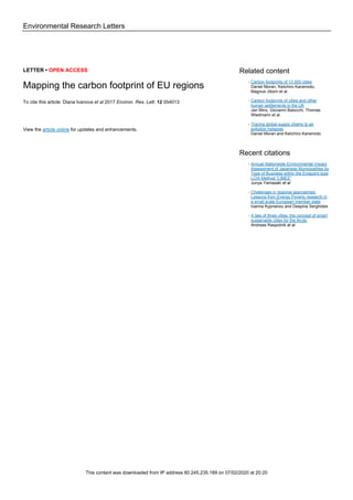
5. constraint at the regional aggregation level. We
conduct relative weights analysis to better understand
the importance of each predictor while addressing the
potential for multicollinearity. We employ cluster-
robust errors to account for the potential correlation
between regional observations belonging to the same
country due to sharing of national features, e.g.
national legislation, institutions, social and cultural
norms, common infrastructure standards etc. Cluster-
robust standard errors have been widely used as a
method to tackle interclass correlation (Cameron and
Miller 2015, Cameron and Trivedi 2009). The
clustered regression approach produces unbiased
clustered standard errors provided that there are a
sufficient number of clusters (Petersen 2009). See the
SI, appendix 1 and 4, for more detailed description of
the variables in the model, statistical procedure and
sensitivity analysis.
3. Results
3.1. Household carbon footprint at subnational level
Figures 1(a) and (b) map total and per capita
household carbon footprint across EU regions.
Descriptive footprint statistics and complete dataset
can be found in the SI. North Rhine-Westphalia and
Bavaria in Germany together emit about 410 MtCO2e
or 40% of German emissions. Other regions with
significant footprints include regions from the UK
(e.g. South East, London), Germany (e.g. Baden-
Württemberg, Lower Saxony), Italy (e.g. Lombardy)
and France (e.g. Parisian Region). Regional footprints
are normally distributed with mean and median of 11
tCO2e/cap and standard deviation of 3 tCO2e/cap. The
top emission decile (i.e. 10% of the population with
highest emissions per capita) includes regions with
average carbon footprint between 22 and 16 tCO2e/
cap. The top decile emits 15% of the total EU
emissions equivalent to 815 MtCO2e. In comparison,
the bottom decile (i.e. 10% of the population with
lowest emissions per capita) make up about 5% of EU
emissions with contribution of 5–7 tCO2e/cap. The
carbon intensity distribution across EU regions is
skewed to the right with a mean, median and standard
deviation of 1.1, 0.9 and 0.4 kgCO2e/EUR BPs,
respectively. The distributions of household carbon
footprints and intensities can be found in SI figure 1.
Countries display different degrees of subnational
heterogeneity. Italy, Spain, Greece and the UK stand
out with the highest footprint ranges. The range refers
to the interval between the lowest and highest regional
estimates within a specific multi regional country
(including outside values). Italy has a range from 6.9 to
13.4 tCO2e/cap, equivalent to 94% of the footprint of
the lowest-impact region, Sicily. Other countries such
as Slovakia and Portugal display lower absolute ranges,
although still substantial when compared to the
magnitude of regional footprints, leading to high
dispersion indices of 0.23 and 0.17 respectively.
Denmark and Czech Republic show the most uniform
distribution of carbon footprints across their regions.
Table 2. CES information by country. Sweden and the Netherlands have been excluded due to lack of regional detail. Only NUTS 1
data available for France, Germany and the UK (larger regions than NUTS 2). For more information about the accuracy, timeliness
and comparability of the surveys refer to the EU quality report (Eurostat 2015b).
EU Countries Year Product detail Spatial detail N Source
Austria 2010 COICOP 2 NUTS 2 9 Household Budget Survey, Statistik Austria
Belgium 2010 COICOP 3 NUTS 2 3 Household Budget Survey, Statistics Belgium
Bulgaria 2010 COICOP 3 NUTS 2 6 Household Budget Survey, NSI
Cyprus 2007 200 products NUTS 2 1 EXIOBASE 2.3
Czech Republic 2011 COICOP 3 NUTS 2 8 Household Budget Survey, Czech Statistical Office
Denmark 2010 COICOP 3 NUTS 2 5 Household Budget Survey, Statistics Denmark
Estonia 2007 200 products NUTS 2 1 EXIOBASE 2.3
Finland 2012 COICOP 3 NUTS 2 5 Household consumption expenditure, Statistics Finland
France 2011 COICOP 3 NUTS 1 9 Household Budget Survey, Insee
Germany 2010 28 products NUTS 1 16 New consumption module, German Socio-Economic Panel
Greece 2014 COICOP 3 NUTS 2 13 Family Budget, EL.STAT
Hungary 2006 COICOP 3 NUTS 2 7 Household Budget Survey, KSH
Ireland 2010 COICOP 3 NUTS 2 2 Household Budget Survey, Central Statistics Office
Italy 2010 COICOP 1 NUTS 2 21 Household Budget Survey, Istat
Latvia 2007 200 products NUTS 2 1 EXIOBASE 2.3
Lithuania 2007 200 products NUTS 2 1 EXIOBASE 2.3
Luxembourg 2007 200 products NUTS 2 1 EXIOBASE 2.3
Malta 2007 200 products NUTS 2 1 EXIOBASE 2.3
Poland 2010 COICOP 1 NUTS 2 16 Household Budget Survey, Central Statistical Office
Portugal 2010 COICOP 3 NUTS 2 7 Household Budget Survey, Statistics Portugal
Romania 2012 COICOP 1 NUTS 2 8 Family Budgets Survey, NIS
Slovakia 2013 COICOP 1 NUTS 2 4 Household Budget Survey, Slovak Statistics
Slovenia 2007 200 products NUTS 1 1 EXIOBASE 2.3
Spain 2010 COICOP 1 NUTS 2 19 Household Budget Survey, INE
United Kingdom 2010 COICOP 4 NUTS 1 12 Living Costs and Food Survey, ONS
Environ. Res. Lett. 12 (2017) 054013
4

6. Table showing within-country absolute and relative
dispersion for the regional totals and by consumption
domain has been included in SI table 2–3 (SI,
appendix 1).
Direct household emissions comprise about 20%
of EU’s household carbon footprint with a ratio
varying between 9%–27% across regions. The
majority of direct emissions are tailpipe emissions
(a) Total household carbon footprint
(MtCO2e)
< 5
5 - 10
10 - 15
15 - 20
20 - 25
25 - 30
30 - 35
35 - 40
40 - 45
45 - 50
> 50
< 5.5
5.5 - 6.8
6.8 - 8.0
8.0 - 9.3
9.3 - 10.5
10.5 - 11.8
11.8 - 13.0
13.0 - 14.3
14.3 - 15.5
15.5 - 16.8
> 16.8
(b) Average household carbon footprint
(tCO2e/cap)
Figure 1. (a) Total household carbon footprint across NUTS 2 regions in MtCO2e (calculated using regional population size from
Eurostat) and (b) per capita household carbon footprint across NUTS 2 regions in tCO2e/cap. National averages of consumption used
for Sweden and the Netherlands, see table 2 for the level of regional detail for the rest. See SI figure 2 for direct-indirect emission
division and appendix 6 for the complete regional dataset. For an interactive version of the per capita map see http://www.
environmentalfootprints.org/regional
Environ. Res. Lett. 12 (2017) 054013
5

7. associated with private use of vehicles. Transport
contributes to about 30% of EU household emissions
with importance across regions varying between
13%–44% with the majority of impacts coming from
burning of transport fuel (see figure 2). Luxembourg
has the highest mobility emissions in Europe with 9.6
tCO2e/cap where emissions from transport fuel
amount to 83% (direct and indirect). Prior analysis
has discussed the potential bias associated with the so-
called tank tourism effect (occurring when residents of
neighbouring countries fill up their tanks in countries
with lower fuel prices); particularly, Luxembourg
stands out with the biggest transport emission
variation between the residence and territory
principle due to price differences in gasoline and
diesel with neighbouring countries, pointing to higher
0 1.25 2.5 3.75 5
Manufactured products and services (tCO2e/cap)
UK
IE
FI
DK
GR
DE
BE
AT
ES
IT
SK
CZ
FR
PT
PL
HU
BG
RO
Clothing
Services
Appliances, machines, electronics
Furniture, household commodities, nec
0 1.25 2.5 3.75 5
Shelter (tCO2e/cap)
UK
IE
FI
DK
GR
DE
BE
AT
ES
IT
SK
CZ
FR
PT
PL
HU
BG
RO
Real estate services
Electricity and fuels
Construction
Waste treatment
0 1.25 2.5 3.75 5
Food (tCO2e/cap)
UK
IE
FI
DK
GR
DE
BE
AT
ES
IT
SK
CZ
FR
PT
PL
HU
BG
RO
Plant−based
Animal−based
Food nec
0 1.25 2.5 3.75 5
Mobility (tCO2e/cap)
UK
IE
FI
DK
GR
DE
BE
AT
ES
IT
SK
CZ
FR
PT
PL
HU
BG
RO
Personal equipment
Transport fuel
Transport services
Figure 2. Subnational distribution of the household carbon footprint by consumption category measured in tCO2e/cap. The graph
excludes all one-region countries and outside values (more than 1.5 Â IQR below or beyond). The boxes describe 25th percentile (left
hinge), median and 75th percentile (right hinge). The adjacent lines describe the min and max (in the absence of outside values).
Countries are ordered by median household carbon footprint. See table 2 for number of regions across countries, SI tables 2–3 for
domain-specific descriptive statistics of within-country absolute and relative dispersion and appendix 5 for product overview across
consumption categories developed in consideration of ISIC detailed structure (United Nations 2017) and household consumption
patterns.
Environ. Res. Lett. 12 (2017) 054013
6

8. uncertainty of results (Usubiaga and Acosta-Fernán-
dez 2015, Statistisches Bundesamt 2010). Transport
fuel emissions are also particularly significant in
France due to commuting to adjacent countries, as
well as Greece and Cyprus, which have large vessel
fleets in proportion to their size resulting in a higher
fuel use of marine bunkers (Usubiaga and Acosta-
Fernández 2015). The contribution of indirect
emissions from private vehicles, other transport
equipment and public transport services is generally
much lower.
Food is a significant source of household emissions
contributing to about 17% of EU household emissions
and a varying importance of 11%–32% across regions.
The capital region of Denmark stands out with the
highest food-related emissions with 3.9 tCO2e/cap or
about27%ofthetotalregionalfootprint.Thesefindings
are in agreement with prior analysis of the Danish
consumption-based emissions embodied in food
(Edjabou and Smed 2013). The largest absolute inter-
regional differences in terms of food emissions occur in
Spain and Greece, where the intervals between the
lowest andhighest regional estimates amount to 1.3and
0.9 tCO2e/cap respectively. This variation is mostly
associated with within-country differences in the
consumption of animal products and processed food.
Animal-based products are associated with higher
magnitude and dispersion of impacts across regions
relative to plant-based products and non-classified food
items. The analysis reveals significant inter-regional
differences in diet composition. For example, animal-
based products contribute to only 33%–38% of food
emissions across regions in Belgium and Denmark,
whileinSloveniasuchproductsbringabout79%offood
emissions.Slovenia also stands out with highest animal-
based emissions per capita in absolute terms, particu-
larly 2.9 tCO2e/cap.
There are significant differences in the way
emissions from clothing and other manufactured
goods are distributed across countries and regions.
Compared to other consumption categories, clothing
contributes to a relatively low share of total household
emissions, only 4% of EU household emissions.
Regions from the UK have some of the highest
emissions associated with clothing in Europe, partic-
ularly, London and Northern Ireland with 0.8 tCO2e/
cap. The relative importance of clothing is highest in
Italy with 5%–7% of carbon impact of consumption.
The UK and Italy demonstrate the highest footprint
range with 0.3 tCO2e/cap. Similar in magnitude and
dispersion is the category of appliances, machinery
and electronics, contributing to 1%–4% of regional
impacts. About 10% of all household emissions in the
EU are associated with other manufactured products,
particularly, furniture, household commodities and
other non-classified items. Emissions from services are
associated with about 14% of the EU’s household
carbon footprint with varying significance across
regions, between 7%–41%. Spain stands out with
higher relative importance of services for the
household carbon footprint, largely associated with
hotel and restaurant services. Similar to transport,
estimates may be biased from improper assignment of
tourist expenditure in EXIOBASE. The services
footprint is highest in the Balearic Islands region
with 4.6 tCO2e/cap, or 41% of the regional emissions.
About 22% of the carbon footprint of EU
households is associated with housing. Direct shelter
emissions comprise about 28% of shelter footprint,
e.g. due to combustion of fuel for heating at home.
The shelter footprint per capita ranges between 1
tCO2e/cap (the Canary Islands) and 5.5 tCO2e/cap
(Åland in Finland) with a rather right-skewed
distribution. Finland stands out with the largest range
of shelter footprint of 1.9 tCO2e/cap. Finnish regions
are classified by the lowest household sizes in our
sample at 1.5 persons per household. In a study of
Finnish households, Heinonen and Junnila (2014)
have confirmed the significance of the economies of
scale effect on energy consumption rates, especially
regarding housing-related emissions. Furthermore,
there are vast differences in terms of the real estate
service footprint, between 5%–58%, suggesting differ-
ences in the way housing impacts (e.g. from
construction) are classified across countries. The
Prague region stands out with a particularly high
shelter footprint from fuel and electricity, 4 tCO2e/cap.
Housing fuel and electricity impacts are rather
significant in the whole of Czech Republic (36%–39%
of household footprint), also characterized by some of
the highest heating degree days and carbon intensity of
the electricity mix (EEA 2011).
As a validity check, regional footprint results have
been scaled up to the national level and compared to
estimates developed using EXIOBASE’s household
demand. Deviations of CES results are within a ten-
percent range from EXIOBASE’s estimates for all
countries in the sample (see SI, appendix 7).
Exceptions are Slovakia and Greece, where the regional
analysis produces footprint results that are 17% and
15% lower than EXIOBASE totals respectively (mostly
due to underestimation of animal-based food and
services emissions). It should be noted that better
consumption detail in terms of COICOP resolution
may be associated with more constrained CES-MRIO
bridge and therefore potentially higher deviation from
EXIOBASE’s estimates.
3.2. Determinants of the household carbon footprint
Table 3 presents the regression output and table 4
supplements it with the raw relative weights and their
significance across model specifications. The point of
this analysis is not to establish causal inference
relationships; the aim is to attempt to explain the
observed regional variation in household carbon
footprints using available NUTS 2 level data for factors
hypothesized to influence carbon footprints and which
have been considered in the literature. Significance
Environ. Res. Lett. 12 (2017) 054013
7

9. level and explanatory power of the factors vary widely
across models.
3.2.1. Socio-economic factors
Income has the highest explanatory power in our
model explaining 29% of the regional household
carbon footprint (table 4). The negative and signifi-
cant quadratic term suggests that the trend is levelling
off. Thus, a thousand-EUR rise in income would result
in roughly 450, 300 and 150 kgCO2e/cap increase in
footprint at the 25th, 50th and 75th income percentile
of the regional sample respectively (at income levels of
Table 3. Regional determinants of household carbon footprint measured in kgCO2e/cap based on 177 EU regions. Dependent
variables from left to right: household carbon footprint of all categories and by food, clothing, mobility, services, manufactured
products, shelter. Cluster-robust standard errors in parenthesis. Significance level: Ã
p < 0.1; ÃÃ
p < 0.05; ÃÃÃ
p < 0.01. Income (in
thousand EUR/cap) and income square term (INC2), household size, predominantly urban (based on population density), tertiary
education (in % of the population aged 30–34 with tertiary education), basic need expenditure (in % of total expenditure), number
of rooms, monthly heating degree days (measuring the severity of the cold on an average month with 15 °C as a heating threshold for
outdoor temperature), forest and semi-natural area (in thousand m2
/cap), electricity mix intensity (categorical variable with the lowest
value of 1 for electricity intensity between 0 and 0.20 kgCO2e/kWh and value of 6 for electricity intensity between 1.0 and 1.2
kgCO2e/kWh). SI table 1 includes a detailed list of sources for all independent variables, while regression results based on other
model specifications and more disaggregated consumption categories are explored in SI tables 6–7. Full regional dataset is included in
appendix 6.
Household carbon
footprint (kgCO2e/cap)
(1) All (2) Food (3) Clothing (4) Mobility (5) Services (6) Manufactured
products
(7) Shelter
INC 644.059ÃÃÃ
7.378 51.643ÃÃÃ
264.515ÃÃÃ
96.533ÃÃÃ
67.497ÃÃ
156.936Ã
(177.49) (57.29) (6.23) (80.90) (32.85) (29.24) (76.25)
INC2
À12.016ÃÃ
0.020 À0.928ÃÃÃ
À3.736 À1.865 À0.824 À4.685ÃÃ
(4.79) (1.73) (0.18) (2.20) (1.13) (0.90) (2.22)
HHSIZE À1276.909 77.490 À58.816 À762.377 508.252Ã
À295.539 À755.106ÃÃ
(1160.14) (250.42) (63.11) (473.35) (291.52) (217.01) (365.84)
URBAN À722.863 À104.976 À8.889 À646.939ÃÃ
À17.306 50.807 5.741
(545.42) (140.14) (24.27) (240.58) (154.98) (69.40) (111.67)
EDUC 62.580ÃÃ
27.704ÃÃÃ
À1.482 11.923 19.215Ã
1.481 3.739
(27.34) (6.48) (1.36) (11.98) (9.82) (5.82) (9.03)
BASIC À75.931Ã
À21.921ÃÃÃ
À0.237 À20.685 À12.606 À13.338 À6.882
(39.23) (7.62) (3.08) (14.44) (8.14) (10.41) (11.52)
NROOMS À1117.122 À16.347 À93.316Ã
À1026.314 332.596 À78.308 À248.821
(1667.34) (410.90) (47.42) (798.23) (464.77) (219.07) (455.33)
HDD
À0.774 À1.467 À0.400 À3.065 À5.846ÃÃÃ
1.394Ã
8.558ÃÃÃ
(5.79) (1.28) (0.24) (2.82) (1.14) (0.81) (1.23)
FORESTAREA
28.994 9.515 À0.213 15.629 32.642ÃÃÃ
À4.159 À24.303ÃÃ
(32.79) (8.76) (1.65) (15.30) (9.56) (5.56) (9.60)
EMIX
847.177ÃÃ
90.228 26.957 77.978 121.967 49.678 481.578ÃÃÃ
(391.68) (77.00) (16.36) (143.15) (100.27) (69.46) (119.69)
Constant 9674.502 2050.048 253.203 5202.427ÃÃ
À284.983 1556.325 922.721
(6456.60) (1434.61) (290.20) (2483.13) (1754.96) (961.31) (1556.35)
R2
0.72 0.51 0.74 0.67 0.69 0.69 0.72
Adjusted R2
0.70 0.48 0.73 0.65 0.67 0.67 0.71
N observations 173 173 173 173 173 173 173
N clusters 25 25 25 25 25 25 25
Table 4. Model summary displaying the raw relative weights of different independent variables across model specifications. The
relative weights sum to the R2
presented in table 3. The significance tests are based on confidence intervals performed with an alpha
value of 0.05 and 10 000 number of iterations for the bootstrapping procedure. Significance level: ÃÃ
p < 0.05.
Predictors (1) All (2) Food (3) Clothing (4) Mobility (5) Services (6) Manufactured
products
(7) Shelter
INC and INC2 0.29ÃÃ
0.03 0.45ÃÃ
0.35ÃÃ
0.09ÃÃ
0.30ÃÃ
0.04ÃÃ
HHSIZE 0.08ÃÃ
0.00 0.09ÃÃ
0.09ÃÃ
0.03ÃÃ
0.11ÃÃ
0.08ÃÃ
URBAN 0.01 0.01 0.01 0.02 0.01 0.02 0.00
EDUC 0.08ÃÃ
0.22ÃÃ
0.01 0.02 0.08ÃÃ
0.03ÃÃ
0.01
BASIC 0.12ÃÃ
0.17ÃÃ
0.03 0.06ÃÃ
0.09ÃÃ
0.09ÃÃ
0.01
NROOMS 0.09ÃÃ
0.04 0.10ÃÃ
0.07ÃÃ
0.08ÃÃ
0.08ÃÃ
0.01
HDD 0.00 0.02 0.04ÃÃ
0.02 0.26ÃÃ
0.04ÃÃ
0.32ÃÃ
FORESTAREA 0.01 0.01 0.00 0.02 0.04ÃÃ
0.00 0.02
EMIX 0.04ÃÃ
0.01 0.02 0.01 0.01ÃÃ
0.01ÃÃ
0.23ÃÃ
Environ. Res. Lett. 12 (2017) 054013
8

10. 8100 EUR/cap, 14 100 EUR/cap and 20 800 EUR/cap
respectively). The income-footprint curve reaches its
peakatanannualnet incomeofaround26800EUR/cap
and starts to decline (within the income range of our
regionalsample).Theconcavenatureoftherelationship
is strongly driven by the domains of clothing and
constructionwithturningpointsof27 800EUR/capand
26 600 EUR/cap respectively. There is a strong linear
effect of income for the domains of services and
manufactured products, where a thousand EUR-
increase in annual income is associated with about
100and70kgCO2e/capemissionrise.Theconsumption
categories of clothing, mobility and manufactured
products appear particularly income-elastic with the
income effect explaining 45%, 35% and 30% of the
regional emission variance respectively. Clothing
registers the highest income elasticity of 0.86.
Increasing the average household size of a region
by one person leads to a drop in the average person’s
emissions associated with electricity and housing fuels
(750 kgCO2e/cap, significant at 5%) and waste
treatment (80 kgCO2e/cap, significant at 5%).
Household size explains 8% of the regional shelter
footprint variance. The urban-rural typology is
insignificant in most of the models except for mobility.
Predominantly urban regions have on average 650
kgCO2e/cap lower emissions from land transport and,
therefore, lower direct and indirect emissions from
transport fuels. Both variables of household size and
urban-rural typology vary little across regions, which
may affect the significance of their effects.
A one-percent point increase in the regional
population with tertiary education is associated with
an increase of about 60 kgCO2e/cap in household
emissions, mainly driven by food consumption. While
the significance of the effect is consistent across all
food sub-categories, the magnitude of the coefficient is
largest for animal-based products according to which a
one-percent point increase in tertiary education is
associated with a 17 kgCO2e/cap rise in animal-based
food footprint. Education explains about 22% of the
variability in regional food emissions, which makes it
the most important factor for that domain in our
model. The basic need ratio ranks second in terms of
importance for food-related emissions, where one-
percent point increase in the regional household
budget on basics brings about a decrease in food-
related emissions of about 20 kgCO2e/cap. The
regression analysis across more disaggregated con-
sumption categories suggests that there are significant
economies of scale driven by dwelling size. An increase
of average dwelling size by one room brings about a
decrease about 130 kgCO2e/cap in both construction
and waste treatment.
3.2.2. Geographic and technical factors
Heating degree days have a positive and highly
significant impact on the regional shelter emissions
explaining more than 30% of the variation in the
dependingvariable.Aone-degreeincreaseintheseverity
of the cold on an average month is associated with an
emission increase of approximately 7 kgCO2e/cap
from housing fuel and electricity use for heating and
2 kgCO2e/cap from both real estate services and
construction. The need for heating is likely lessened
by the more stricter building standards enforced in
northern European countries where households con-
sume less energy for heating per unit floor area and
heating degree day (Balaras et al 2007). Moderately
increased emissions from heating in colder regions are
offset by lower emissions embodied in services,
particularly hotel and restaurant services. A rise in the
forest area of a region by a thousand square meters per
capita is associated with a 40 kgCO2e/cap drop in
electricity and housing fuel emissions. Households have
been noted to consume more resources when they are
readily available (Ivanova et al 2015) suggesting that
availability of forest products may encourage the use of
woodfor heating, which isassumedtobecarbon neutral
in EXIOBASE.
The electricity mix intensity explains an additional
23% of the variance in shelter emissions. An increase
in the electricity mix intensity by 0.2 kgCO2e/kWh
results in a rise of housing impacts of 480 kgCO2e/cap.
The majority of this effect (about 80%) can be
explained by changes in the regional footprint
associated with electricity and housing fuels, though
significant effect is noted for the energy-intensive sub-
categories of real estate services and construction as
well. This factor captures the carbon intensity of the
domestic electricity mix and, therefore, its effect would
be proportionate to the share of domestically
produced consumption.
4. Discussion
This is the first study to quantify region-level
consumption-based GHG emissions associated with
household consumption in a comprehensive frame-
work across the European Union. It combines the use
of regionalized consumer expenditure data with
multiregional input-output framework to trace carbon
impacts along global supply chains and highlights the
most carbon-contributing consumption activities
across regions. The regression analysis allows to test
potential effects identified from other groupings of the
CES data on the regional aggregate level. Prior studies
have emphasized the need for a broader international
comparative perspective in the examination of social
driving forces of emissions (Rosa and Dietz 2012).
Socio-economic factors such as income, house-
hold size, education, dwelling size and basic con-
sumption generally explain between 15%–69% of the
subnational heterogeneity (11%–44% excluding in-
come) in emissions with their statistical significance
varying widely across regression models. Countries
with higher inter-regional income inequality (e.g. Italy,
Environ. Res. Lett. 12 (2017) 054013
9

11. the UK and Spain) also stand out with wider emission
ranges consistent across consumption domains,
particularly income-elastic domains such as clothing,
services and manufactured products. These results are
in line with previous findings suggesting that macro-
trends in GHG emissions are heavily driven by socio-
economic factors, while geographic and infrastructural
effects have limited effect on the regional level of
analysis (Minx et al 2013, Baiocchi et al 2010). Income
has a varying significance across consumption
domains. Prior studies have suggested that rising
affluence may shift the composition of consumption
(not only the scale) and, thus, it may or may not
compensate for the tendency that increased affluence
comes at increased GHG emissions (Rosa and Dietz
2012). In an EU27 country panel, Sommer and
Kratena (2016) also find a relative decoupling effect
due to a higher saving rate and less emission intensive
consumption of top income quintiles, which however
does not compensate for the much higher levels of
consumption. We find a stronger evidence for levelling
off of the emission-income curve rather than turning
points (i.e. the so-called environmental Kuznets curve
hypothesis) with only a small fraction of the regional
sample lying beyond the suggested threshold of 26 800
EUR annual individual income (< 3%). It has been
suggested that thresholds instead signal for critical
points differentiating between different income groups
of countries (Liao and Cao 2013).
Shelter and mobility demonstrate rather high
regional dependence with an emission share ranging
between 10%–46% and 13%–44% respectively.
Impacts from housing and transport dominate
countries such as Austria, Denmark and France (with
regional mobility footprints between 2.8–5.2 tCO2e/
cap), Finland, Poland and Czech Republic (with
regional shelter footprint between 3.0–5.5 tCO2e/cap),
Bulgaria and Hungary (both shelter and mobility).
Prior literature has suggested that increases in
household size reduce emissions per capita and
increase eco-efficiency, most pronounced in the
housing domain (Tukker et al 2010, Weber and
Matthews 2008, Wilson and Boehland 2005). This is in
agreement with our results as we find a negative
and highly significant effect of household size
particularly in the domain of shelter. Our regional
analysis does not confirm prior hypotheses that urban
residents and smaller dwelling sizes contribute to
lower housing impacts due to the dwelling structure
(Tukker et al 2010, Lenzen et al 2006). Nevertheless,
the insignificance of the variables may be a result of the
large and mixed (in terms of urban-rural typology)
regions and housing price differences between densely
and sparsely populated areas. Additional factors with
potential importance include characteristics of the
dwelling stock (e.g. type, age and level of refurbish-
ment), residential floor area, types of construction
materials and fuels used and proportion of combined
heat and power generation among others (Wilson et al
2013a, Tukker et al 2010). Selected geographic and
technical factors explain up to 34% and 23%
respectively of the regional shelter-related emissions,
thus, outweighing the importance of socio-economic
controls for the shelter domain. It has been previously
suggested that geographic and infrastructural effects
may be more significant at a finer spatial detail (Minx
et al 2013).
Income is the single most important determinant
of transport emissions explaining 35% of their
variation, where a rise in individual annual income
of a thousand EUR increases emissions by about 265
kgCO2e. Predominantly urban households contribute
to about 650 kgCO2e/cap less on average compared to
their rural counterparts on the regional level of data
aggregation. Prior studies have signalled that denser
urban forms are associated with lower GHG emissions
from road passenger transport, but potentially higher
contribution from air travel and other passenger
transportation (Jones and Kammen 2015, Ottelin et al
2014, Ornetzeder et al 2008). A systematic bias may
arise if air travel is under-reported in consumer
expenditure surveys as an infrequent purchase (Bee et
al 2015). Additional private and institutional indica-
tors expected to affect regional transport-related
emissions include private vehicle ownership and
technical characteristics of the vehicle fleet, density
of road network, public transport availability and
proximity to an airport (Waisman et al 2013, Tukker et
al 2010). The exclusion of such factors from the model
may give rise to omitted variable bias.
Food emissions are rather income inelastic. They
vary between 1.0 and 3.9 tCO2e/cap across regions
with an impact share of 11%–32%. Similar spatial
invariability of environmental food-related impacts
has been shown for the neighbourhood level in
Canada and the USA (Wilson et al 2013a, Jones and
Kammen 2015). Basic consumption share is associated
with lower food emissions when controlling for
income. This effect may occur due to a shift of
spending from food to shelter in order to offset rising
utilities expenditures for low-income households
(Schanzenbach et al 2016, Bhattacharya et al 2003)
and carbon intensity differences between basic and
discretionary spending (Ivanova et al 2015). A one-
percent point rise in the population with tertiary
education brings about an increase in the regional
food footprint of close to 30 kgCO2e/cap, where
education explains about 22% of the variation in
regional food-embodied emissions. Duarte et al
(2012) also found better educated households to
contribute to higher consumption and GHG emis-
sions than less educated ones, although at a lower
emission intensity of consumption. Our results
confirm the generally uncertain direction of the
education effect previously outlined by Chancel and
Piketty (2015).
We have already discussed the potential for
omitted variable bias due to limited availability of
Environ. Res. Lett. 12 (2017) 054013
10

12. data on NUTS level. Such omitted factors include
institutions (e.g. demographic institutions of gover-
nance leading to greater environmental protection),
social psychology and culture (e.g. values, beliefs,
norms and world-views) (Rosa and Dietz 2012).
There are certain limitations to our method with
regards to footprint calculations. CESs provide no
physical layer of consumption or price information, so
we apply average product intensities. This may cause a
systematic bias in our analysis as luxurious consump-
tion has potentially lower resource intensity per unit
expenditure than mass-produced products of the same
category (Hertwich 2005). Sectors classified by a larger
gap between residence and territory estimates such as
tourism and transport sectors are likely associated with
higher uncertainty of results. Whilst a systematic
assessment of uncertainty is not feasible here (CES
data had no uncertainty estimates associated with it),
national level studies point to uncertainty ranges of
about 5%–10% for carbon footprints (Lenzen et al
2010, Karstensen et al 2015, Moran and Wood 2014),
with relatively higher uncertainty for smaller econo-
mies, or in the context of this study, regional
populations. With regards to the statistical analysis,
our dataset is relatively non-uniform across countries
with varying number of regions, survey collection
years and consumption detail. The size of the regions
may be too large to allow for significant variation of
socio-economic, geographic and technical factors.
Prior research has also signalled for the modifiable
areal unit problem according to which spatial
aggregation of grouping of data comes at the price
of inevitable loss of information or bias (Wong 2009).
Our study provides comprehensive insights into
the subnational spatial variation of household carbon
footprints and allows regions to monitor consump-
tion-based emissions and consider them when setting
priorities for climate policies. Ultimately, regions differ
in their emissions and reduction potential, which also
implies differences in their climate responsibility for
national mitigation strategies.
Acknowledgments
This work is an output of the GLAMURS project
financed by the European Union’s seventh framework
program (contract 613420). The EXIOBASE database
was constructed in the CREEA project, financed by the
same program (contract 265134). The authors thank
Radek Lonka for technical and graphics assistance and
Nancy Lea Eik-Nes for writing assistance and language
editing. Data collection for the study was enabled by
national statistical offices; special thanks to Irina
Macsinga, Statistics Greece and the German Socio-
Economic Panel for data acquisition in the cases when
region-level consumption information was less accessi-
ble.
References
Adom F, Maes A, Workman C, Clayton-Nierderman Z, Thoma
G and Shonnard D 2012 Regional carbon footprint
analysis of dairy feeds for milk production in the USA Int.
J. Life Cycle Assess. 17 520–34
Aichele R and Felbermayr G 2015 Kyoto and carbon leakage: an
empirical analysis of the carbon content of bilaterial trade
Rev. Econ. Stat. 97 104–15
Aichele R and Felbermayr G 2012 Kyoto and the carbon
footprint of nations J. Environ. Econ. Manage. 63 336–54
Andonova L B and Mitchell R B 2010 The rescaling of global
environmental politics Annu. Rev. Environ. Resour. 35
255–82
Baiocchi G, Minx J and Hubacek K 2010 The impact of social
factors and consumer behaviour on carbon dioxide
emissions in the United Kingdom J. Ind. Ecol. 14 50–72
Balaras C A, Gaglia A G, Georgopoulou E, Mirasgedis S,
Sarafidis Y and Lalas D P 2007 European residential
buildings and empirical assessment of the hellenic building
stock, energy consumption, emissions and potential energy
savings Build. Environ. 42 1298–314
Bee A, Meyer B D and Sullivan J X 2015 The validity of
consumption data: are the consumer expenditure interview
and diary surveys informative? Improving the Measurement
of Consumer Expenditures ed C D Carroll, T F Crossley and
J Sabelhaus (Chicago and London: University of Chicago
Press) pp 204–40 (www.nber.org/chapters/c12662.pdf)
Bhattacharya J, DeLeire T, Haider S and Currie J 2003 Heat or
eat? Cold-weather shocks and nutrition in poor American
families Am. J. Public Health 93 1149–54
Cameron C and Miller D L 2015 A practitioner’s guide to
cluster-robust inference J. Hum. Resour. 50 317–72
Cameron C and Trivedi P 2009 Microeconometrics Using Stata
(College Station, TX: Stata Press)
Chancel L and Piketty T 2015 Carbon and Inequality: from
Kyoto to Paris (Paris School of Economics) (piketty.pse.
ens.fr/files/ChancelPiketty2015.pdf)
Curry R and Maguire C 2011 The use of ecological and carbon
footprint analysis in regional policy making: application
and insights using the REAP model Local Environ. Int. J.
Justice Sustain. 16 917–36
Deng G, Ma Y and Li X 2016 Regional water footprint
evaluation and trend analysis of China—based on
interregional input–output model J. Clean. Prod. 112
4674–82
Duarte R, Mainar A and Sanchez-Choliz J 2012 Social groups
and CO2 emissions in Spanish households Energ. Policy 44
441–50
Edjabou L D and Smed S 2013 The effect of using consumption
taxes on foods to promote climate friendly diets—the case
of Denmark Food Policy 39 84–96
EEA 2011 CO2 (g) per KWh in 2009 (electricity only) (http://
www.eea.europa.eu/data-and-maps/figures/co2-electricity-g-
per-kwh/co2-per-electricity-kwh-fig-1_2010_qa.xls)
(Accessed: 2 April 2017)
European Commission 2011a A resource-efficient Europe—
Flagship Initiative under the Europe 2020 Strategy
(Brussels: European Commission) (http://ec.europa.eu/
resource-efficient-europe/index_en.htm)
European Commission 2016 Climate strategies and targets: 2020
climate and energy package (http://ec.europa.eu/clima/policies/
strategies/2020/index_en.htm) (Accessed: 8 July 2016)
European Commission 2011b Regional Policy Contributing to
Sustainable Growth in Europe 2020 (Brussels) (http://eur-
lex.europa.eu/legal-content/EN/TXT/?qid=1399618687721
&uri=CELEX:52011DC0017)
European Communities 2003 Household Budget Surveys in the
EU: Methodology and Recommendations for Harmonisation
(Luxembourg: European Commission) (ec.europa.eu/
eurostat/ramon/statmanuals/files/KS-BF-03-003-__-N-EN.
pdf)
Environ. Res. Lett. 12 (2017) 054013
11

13. Eurostat 2017 Glossary: Nomenclature of territorial units for
statistics (NUTS) (http://ec.europa.eu/eurostat/statistics-
explained/index.php/Glossary:Nomenclature_of_
territorial_units_for_statistics_(NUTS)) (Accessed: 20
February 2017)
Eurostat 2016 Greenhouse gas emission statistics (http://ec.europa.
eu/eurostat/statistics-explained/index.php/Greenhouse_gas_
emission_statistics)
Eurostat 2015a HICP (2005 ¼ 100)—annual data (average index
and rate of change) (http://ec.europa.eu/eurostat/web/hicp/
data/database) (Accessed: 5 April 2017)
Eurostat 2015b Household Budget Survey. 2010 Wave (http://ec.
europa.eu/eurostat/web/household-budget-surveys/
publications)
Girod B, van Vuuren D P and Hertwich E G 2014 Climate policy
through changing consumption choices: options and
obstacles for reducing greenhouse gas emissions Glob.
Environ. Change 25 5–15
Godar J, Persson U M, Tizado E J and Meyfroidt P 2015
Towards more accurate and policy relevant footprint
analyses: tracing fine-scale socio-environmental impacts of
production to consumption Ecol. Econ. 112
25–35
Harris P G, Chow A S Y and Symons J 2012 Greenhouse gas
emissions from cities and regions: international
implications revealed by Hong Kong Energ. Policy 44
416–24
Heinonen J and Junnila S 2014 Residential energy consumption
patterns and the overall housing energy requirements of
urban and rural households in Finland Energ. Build. 76
295–303
Hertwich E G 2005 Life cycle approaches to sustainable
consumption: a critical review Environ. Sci. Technol. 39
4673–84
Hertwich E G and Peters G P 2009 Carbon footprint of nations:
a global, trade-linked analysis Environ. Sci. Technol. 43
6414–20
Ivanova D, Stadler K, Steen-Olsen K, Wood R, Vita G, Tukker A
and Hertwich E G 2015 Environmental impact assessment
of household consumption J. Ind. Ecol. 20 526–36
Jackson T and Papathanasopoulou E 2008 Luxury or ‘lock-in’?
An exploration of unsustainable consumption in the UK:
1968 to 2000 Ecol. Econ. 68 80–95
Jones C M and Kammen D M 2015 A consumption-based
greenhouse gas inventory of San Francisco Bay Area
neighborhoods, cities and counties: Prioritizing climate
action for different locations (https://escholarship.org/uc/
item/2sn7m83z)
Jones C M and Kammen D M 2011 Quantifying carbon
footprint reduction opportunities for U.S. households and
communities Environ. Sci. Technol. 45 4088–95
Jones C M and Kammen D M 2014 Spatial distribution of US
household carbon footprints reveals suburbanisation
undermines greenhouse gas benefits of urban population
density Environ. Sci. Technol. 48 895–902
Karstensen J, Peters G P and Andrew R M 2015 Uncertainty in
temperature response of current consumption-based
emissions estimates Earth Syst. Dyn. 6 287–309
Larsen H N and Hertwich E G 2011 Analyzing the carbon
footprint from public services provided by counties J.
Clean. Prod. 19 1975–81
Lenzen M, Dey C J and Foran B 2004 Energy requirements of
Sydney households Ecol. Econ. 49 375–99
Lenzen M, Wier M, Cohen C, Hayami H, Pachauri S and
Schaeffer R 2006 A comparative multivariate analysis of
household energy requirements in Australia, Brazil,
Denmark, India and Japan Energy 31 181–207
Lenzen M, Wood R and Foran B 2008 Direct versus embodied
energy—the need for urban lifestyle transitions Urban
Energy Transition: From Fossil Fuels to Renewable Power ed
P Droege (Amsterdam: Elsevier BV) pp 91–120
Lenzen M, Wood R and Wiedmann T 2010 Uncertainty analysis
for multi-region input—output models—a case study of
the UK’s carbon footprint Econ. Syst. Res. 22
43–63
Liao H and Cao H S 2013 How does carbon dioxide emission
change with the economic development? Statistical experiences
from 132 countries Glob. Environ. Change 23 1073–82
Lin T, Yu Y, Bai X, Feng L and Wang J 2013 Greenhouse gas
emissions accounting of urban residential consumption: a
household survey based approach PLoS One 8 e55642
Marcotullio P J, Sarzynski A, Albrecht J and Schulz N 2014 A
top-down regional assessment of urban greenhouse gas
emissions in Europe Ambio 43 957–68
Meng B, Xue J, Feng K, Guan D and Fu X 2013 China’s inter-
regional spillover of carbon emissions and domestic supply
chains Energ. Policy 61 1305–21
Miehe R, Scheumann R, Jones C M, Kammen D M and Finkbeiner
M 2016 Regional carbon footprints of households: a German
case study Environ. Dev. Sustain. 18 577–91
Minx J, Baiocchi G, Wiedmann T, Barrett J, Creutzig F, Feng K,
Förster M, Pichler P-P, Weisz H and Hubacek K 2013
Carbon footprints of cities and other human settlements in
the UK Environ. Res. Lett. 8 035039
Minx J C et al 2009 Input–output analysis and carbon
footprinting: an overview of applications Econ. Syst. Res.
21 187–216
Moran D and Wood R 2014 Convergence between the EORA,
WIOD, EXIOBASE, and OPENEU’s consumption-based
carbon accounts Econ. Syst. Res. 26 245–61
Newton P and Meyer D 2012 The determinants of urban
resource consumption Environ. Behav. 44 107–35
Ornetzeder M, Hertwich E G, Hubacek K, Korytarova K and
Haas W 2008 The environmental effect of car-free
housing: a case in Vienna Ecol. Econ. 65 516–30
Ottelin J, Heinonen J and Junnila S 2014 Greenhouse gas
emissions from flying can offset the gain from reduced
driving in dense urban areas J. Transp. Geogr. 41 1–9
Peters G P and Hertwich E G 2008 CO2 embodied in
international trade with implications for global climate
policy Environ. Sci. Technol. 42 1401–7
Petersen M A 2009 Estimating standard errors in finance panel data
sets: comparing approaches Rev. Financ. Stud. 22 435–80
Rosa E A and Dietz T 2012 Human drivers of national
greenhouse-gas emissions Nat. Clim. Change 2 581–6
Sanne C 2002 Willing consumers—or locked-in policies for a
sustainable consumption Ecol. Econ. 42 273–87
Schanzenbach D W, Nunn R, Bauer L and Mumford M 2016
Where does all the money go: Shifts in household spending
over the past 30 years (www.hamiltonproject.org/papers/
where_does_all_the_money_go_shifts_in_household_
spending_over_the_past_30_y)
Skelton A 2013 EU corporate action as a driver for global
emissions abatement: a structural analysis of EU
international supply chain carbon dioxide emissions Glob.
Environ. Change 23 1795–806
Solomon S, Qin D, Manning M, Marquis M, Averyt K, Tignor
M M B LeRoy Miller H and Chen Z 2007 Contribution of
Working Group I to the Fourth Assessment Report of the
Intergovernmental Panel on Climate Change: Climate
change 2007 The Physical Science Basis (Cambridge:
Cambridge United Press) (www.ipcc.ch/report/ar4/wg1/)
Somanathan E et al 2015 National and sub-national policies and
institutions Climate Change 2014: Mitigation of Climate
Change ed O Edenhofer (Cambridge: Cambridge
University Press) pp 1141–206
Sommer M and Kratena K 2016 The carbon footprint of European
households and income distribution Ecol. Econ. 136 62–72
Stadler K, Steen-Olsen K and Wood R 2014 The ‘rest of the
world’—estimating the economic structure of missing
regions in global multi regional input–output tables Econ.
Syst. Res. 26 303–26
Environ. Res. Lett. 12 (2017) 054013
12

14. Statistisches Bundesam 2010 Energy consumption and CO2
emissions of road transport as part of the NAMEA
compilation strategy (www.destatis.de/EN/Publications/
Specialized/EnvironmentalEconomicAccounting/
TransportAndEnviroment/Transport5859004109004.pdf?
__blob=publicationFile)
Steen-Olsen K, Wood R and Hertwich E G 2016 The carbon
footprint of Norwegian household consumption 1999–2012
J. Ind. Ecol. 20 582–92
Tukker A, Bulavskaya T, Giljum S, de Koning A, Lutter S, Simas M,
Stadler K and Wood R 2016 Environmental and resource
footprints in a global context: Europe’s structural deficit in
resource endowments Glob. Environ. Change 40 171–81
Tukker A, Cohen M J, Hubacek K and Mont O 2010 The
impacts of household consumption and options for change
J. Ind. Ecol. 14 13–30
Turner K, Munday M, McIntyre S and Jensen C D 2011
Incorporating jurisdiction issues into regional carbon
accounts under production and consumption accounting
principles Environ. Plan. A 43 722–41
United Nations 2017 International standard industrial
classification of all economic activities, Rev.3.1 (ISIC
Rev.3.1) (http://unstats.un.org/unsd/cr/registry/regcst.asp?
Cl=17) (Accessed: 5 April 2017)
Usubiaga A and Acosta-Fernández J 2015 Carbon emission
accounting in MRIO models: the territory vs. the residence
principle Econ. Syst. Res. 27 458–77
Waisman H-D, Guivarch C and Lecocq F 2013 The
transportation sector and low-carbon growth pathways:
modelling urban, infrastructure, and spatial determinants
of mobility Clim. Policy 13 106–29
Weber C L and Matthews H S 2008 Quantifying the global and
distributional aspects of American household carbon
footprint Ecol. Econ. 66 379–91
Wiedenhofer D, Lenzen M and Steinberger J K 2013 Energy
requirements of consumption: Urban form, climatic and
socio-economic factors, rebounds and their policy
implications Energ. Policy 63 696–707
Wilson A and Boehland J 2005 Small is beautiful: US household
size, resource use, and the environment J. Ind. Ecol. 9
277–87
Wilson J, Tyedmers P and Grant J 2013a Measuring
environmental impact at the neighbourhood level J.
Environ. Plan. Manag. 56 42–60
Wilson J, Tyedmers P and Spinney J E L 2013b An exploration
of the relationship between socioeconomic and well-being
variables and household greenhouse gas emissions J. Ind.
Ecol. 17 880–91
Wong D 2009 The modifiable areal unit problem (MAUP) The
SAGE Handbook of Spatial Analysis ed S A Fotheringham
and P A Rogerson (London: SAGE Publications Ltd) pp
105–23
Wood R and Dey C J 2009 Australia’s carbon footprint Econ.
Syst. Res. 21 243–66
Wood R and Garnett S 2009 An assessment of environmental
sustainability in Northern Australia using the ecological
footprint and with reference to indigenous populations
and remoteness Ecol. Econ. 68 1375–84
Wood R and Garnett S 2010 Regional sustainability in
Northern Australia—a quantitative assessment of social,
economic and environmental impacts Ecol. Econ. 69
1877–82
Wood R, Hawkins T R, Hertwich E G and Tukker A 2014
Harmonising national input—output tables for
consumption-based accounting—experiences from
EXIOPOL Econ. Syst. Res. 26 387–409
Wood R et al 2015 Global sustainability accounting—developing
EXIOBASE for multi regional footprint analysis
Sustainability 7 138–63
Zhang C and Anadon L D 2014 A multi regional input-output
analysis of domestic virtual water trade and provincial
water footprint in China Ecol. Econ. 100 159–72
Zhou X and Imura H 2011 How does consumer behavior
influence regional ecological footprints? An empirical
analysis for Chinese regions based on the multi-region
input-output model Ecol. Econ. 71 171–9
Environ. Res. Lett. 12 (2017) 054013
13