ل

1. 1 | P a g e
COE 588: Modeling and Simulation
Term 191
Course Project
Final Report
Project Title:
Performance Analysis of SSQ System under DoS attacks
Team members:
Reference:
S. Khan and I. Traore, "Queue-based analysis of DoS attacks," Proceedings from the Sixth
Annual IEEE SMC Information Assurance Workshop, West Point, NY, USA, 2005, pp. 266-
273. doi: 10.1109/IAW.2005.1495962
What is the research problem tackled in the paper?
§ The behavior of Single Server Queuing(SSQ) system under Denial-of-service (DoS)
attacks. (i.e. flooding attacks and complexity attacks).
What are the objective(s) of the author(s)?
§ Study the impact of flooding and complexity attacks on the performance metrics
(queue growth-rate, and response time).
What are the research questions to be answered?
§ What are the impacts of flooding and complexity attacks on the queue-growth-rate,
and response time?
§ Can the average queue-growth-rate, and average response time of requests metrics
be used to predict such DoS attacks?
What research methodology is used in the paper?
In the main paper:
§ Mathematical (Analytical) model and
§ Experimental setup to validate his mathematical model.
While, we use:
Simulation Model to validate his objectives and the mathematical model.
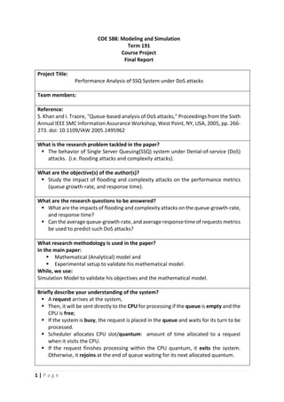
Briefly describe your understanding of the system?
§ A request arrives at the system,
§ Then, it will be sent directly to the CPU for processing if the queue is empty and the
CPU is free;
§ If the system is busy, the request is placed in the queue and waits for its turn to be
processed.
§ Scheduler allocates CPU slot/quantum: amount of time allocated to a request
when it visits the CPU.
§ If the request finishes processing within the CPU quantum, it exits the system.
Otherwise, it rejoins at the end of queue waiting for its next allocated quantum.

2. 2 | P a g e
Describe the conceptual model of the system (i.e., entities, attributes, state
variables, events, and activities).
Table 1: The items of our conceptual model
Model Description
Entities Queue, CPU, Requests
Attributes Arrival time, Exit time, Remaining service time
State Variables Q: Number of requests in the queue, Q ∈ {0, 1, 2, …}
S: CPU state, S ∈ {Free, Busy}
Events Start, Arrival, Admitted, start service, Departure, and Exit
Activities Generation, Waiting, Service, Delay
Draw the queueing model of the system (if possible).
Fig. 1: Queueing model of our system.
Draw the Event Graph
Fig. 2: Event graph of our system.
Description:
Obviously, we have here 6 main events: Start, Arrival, Admitted, Start Service,
Departure, and Exit. The system will start from the first event (“Start”) by initializing the
Queue value (Q=0) and free the server (S=0). Then, the request will arrive the system
after time value (ta) and got admitted directly to the tail of the Queue and updated the
value of Q by Q+1. In the meantime, if there are no requests currently in the Queue and
the server is free, it will generate directly a “Start Service Event” and update the state
of Queue by (Q-1) and the server (S=1). Next, the “Start Service Event” will fetch the
next request in the Queue and schedule a “Departure Event” for the request after time

3. 3 | P a g e
value equal “Quantum + context switch time”. In this graph, we assume that the request
length is equal to multiple CPU quantum.
The Departure Event will update the remaining service time of the request and the
Server status. It will then schedule either an Exit or Admitted Event based on the
remaining service time of the request. In either case, the Departure Event will schedule
a Start Service Event if the Queue is not empty.
Since Start Service and Admitted Events can be scheduled at the same clock time, the
events need to be prioritized. The events are prioritized as follows (highest to lowest):
Start Service, Exit, Admitted, Departure, and Arrival.
List of performance metrics used in the study along with their definitions.
§ Queue Growth-Rate: average increase in queue size in time unit.
Queue-growth-rate = Queue size at end of simulation / total simulation time.
§ Average Response Time: average of the response times for all simulated requests.
Response Time = Exit time - Arrival time.
Give the definitions of output variables for each performance metric (i.e., raw data to
be collected in order to estimate the value of the performance metric).
§ Queue Growth-Rate:
Output Variable: size of queue at the end of simulation.
§ Average Response Time:
Output Variables: for each simulated request: arrival time and exit time.

4. 4 | P a g e
Simulation Results
Event-Driven Simulation Stages:
Fig. 3: Event Driven Simulation Program Steps.
Our simulation program is divided into the following four parts:
1. Initialization:
We initialized and selected the suitable values of our parameters for each single
experiment: Simulation Time, Quantum, Context Switch Time, Average Request
Service Length, Request Arrival Rate, and State Variables.
2. Simulation Loop:
We used the simulation time as the stopping condition in our simulation loop,
and events will be executed based on our simulation time.
3. Model:
Our model contains the following event handlers: Arrival, Admitted, Start
Service, Departure, and Exit. Also, it contains a corresponding event generator
for each handler.
4. Output:
We store the queue size value at the end of simulation to calculate the queue
growth rate. In addition, we store the arrival and exit times for each simulated
request to calculate the average response time.

5. 5 | P a g e
The simulation results of our performance metrics versus the system parameters are
given below:
1. Queue-growth rate vs Arrival Rate:
§ Parameters:
CPU Quantum: 0.01 sec,
Context Switch Time = 0.002 sec,
Simulation runs = 10,
Simulation time = 10 secs,
L: average number of CPU quantum needed by a request = {1, 2, and 6} (
average service time = L x 0.01),
Arrival rate (lamda) = [1,2, 3, … ,200].
§ Chart:
Fig.4 shows the relation between the queue growth rate and the arrival rate
for different request lengths {1, 2, and 6}. In this figure, each point represents
one experiment. It is clearly shown from the graph that there are two regions
for each L value. In the first region, the queue growth rate is zero which implies
a normal system behavior. However, in the second region the queue growth
rate increases linearly as Lambda increases. For instance, consider the curve
where L=1. The queue growth rate remains zero while lambda is less than 80.
Then, queue growth rate increases linearly as the value of lambda increases.
The figure also shows that the behavior (line slope) is similar for different values
of L. However, increasing the L value, will decrease the normal behavior period
with respect to lambda, and it will increase the queue growth rate.
Fig. 4: Queue growth rate vs arrival rate

6. 6 | P a g e
2. Queue-growth rate vs Request Length:
§ Parameters:
CPU Quantum: 0.01 sec,
Context Switch Time = 0.002 sec,
Simulation runs = 100,
Simulation time = 10 secs,
L: average number of CPU quantum needed by a request = [1,2,3, …, 200] (
average service time = L x 0.01),
Arrival rate (lamda) = {2, 3, 5, and 6}.
§ Chart:
Fig.5 shows the relation between the queue growth rate and the request length
for different arrival rates (lamda) {2, 3, 5, and 6}. In this figure, each point
represents one experiment. The figure shows that the queue growth rate
remains zero for a very short range of L values, which represents a normal
behavior of the system. Then, it will increase with the increment of the request
length until it reaches a certain value. After that, the rate of increase gradually
decreases, as the value of L becomes larger. When L becomes very large, the
queue growth rate will reach to a constant value.
For instance, consider the curve where Lambda = 5. The queue growth rate
remains zero while L is less than 10. Then, the queue growth rate increases as
the value of L increases until it reaches the value of 75. When L becomes
greater than 75, the rate of increase in the queue growth rate will gradually
decrease until it reaches a constant value.
The figure also shows that the behavior is similar for different values of Lamda.
However, increasing the Lambda value, will decrease the normal behavior
period with respect to L, and it will increase the queue growth rate.
Fig. 5: Queue growth rate vs request length

7. 7 | P a g e
3. Average Response Time vs Arrival Rate:
§ Parameters:
CPU Quantum: 0.01 sec,
Context Switch Time = 0.002 sec,
Simulation runs = 10,
Simulation time = 10 secs,
L: average number of CPU quantum needed by a request = {1, 2, and 6}
(average service time = L x 0.01),
Arrival rate (lamda) = [1,2,3,…, 200].
§ Chart:
Fig.6 shows the relation between the average response time and the arrival
rate for different request lengths {1, 2, and 6}. Each point in this figure
represents one experiment. The figure shows that the average response time
remains stable for a certain range of Lambda values, which represents a normal
behavior of the system where the average response time is almost equal to the
request length. Then, it will increase as the value of lambda increases. For
instance, consider the curve where L=2. The average response time is almost
equal to 𝐿 × 0.01 = 0.02 while lambda is less than 25. Then, the average
response time increases as the value of lambda increases.
The figure also shows that the behavior is similar for different values of L.
However, increasing the L value, will decrease the stable behavior period with
respect to lambda, and it will increase the average response time.
Fig. 6: Average response time vs arrival rate

8. 8 | P a g e
4. Average Response Time vs Request Length:
§ Parameters:
CPU Quantum: 0.01 sec,
Context Switch Time = 0.002 sec,
Simulation runs = 10,
Simulation time = 100 secs,
L: average number of CPU quantum needed by a request = [1,2,3,…,200](
average service time = L x 0.01),
Arrival rate (lamda) = {2, 3, 5, and 6}.
§ Chart:
Fig.7 shows the relation between the average response time and the request
length for different arrival rates {2, 3, 5, and 6}. Each point in this figure
represents one experiment. The figure shows that the average response time
remains stable for a certain range of L values, which represents a normal
behavior of the system where the average response time is almost equal to the
request length (L x CPU Quantum). Then, it will increase with the increment of
the request length until it reaches a certain value. After that, the rate of
increase gradually decreases, as the value of L becomes larger.
For instance, consider the curve where Lambda = 6. The average response time
is almost equal to 𝐿 × 0.01 while L is less than 10. Then, the average response
time increases as the value of lambda increases until it reaches the value of 50.
When L becomes greater than 50, the rate of increase in the average response
time will gradually decrease.
Fig. 7: Average response time vs request length

9. 9 | P a g e
Discussion
The comparison between our simulation results obtained from our simulation model
with the graphs reported in the paper are given below:
1. Queue-growth rate vs Arrival Rate:
From Fig.8, we notice that our results match the authors’ results for all L values.
As we discussed in the previous section, the curves start with zero growth rate
and then it increases while the arrival rate is increasing in a linear relation.
We can conclude from this figure that the strong flooding attacks have high
impact on the queue growth rate. The impact of flooding attacks linearly
increases as the arrival rate increases.
Fig. 8: Queue-growth rate vs Arrival Rate, authors’ results (left), our results (right)
2. Queue-growth rate vs Request Length:
From Fig.9, we notice that our results match the authors’ results for all arrival
rate values. As we discussed in the previous section, the curves start with zero
queue growth rate, and then it will increase as the request length increases until
it reaches a certain value. After that, the rate of increase gradually decreases, as
the value of L becomes larger. When L becomes very large, the queue growth
rate will reach to a constant value.
Fig. 9: Queue growth rate vs. request length: authors’ results (left), our results (right)

10. 10 | P a g e
The constant value that the queue growth rate will reach represents the value of
the arrival rate. This can be explained as follows: when L becomes very large, the
request will stay for a very long time in the system. In the meantime, new
requests will arrive in every second according the average arrival rate. Therefore,
no requests will leave the system, and the queue size will be incremented each
second by the value of the arrival rate.
The authors also validated this behavior through their developed mathematical
model. The validation is based on the queue growth rate formula:
𝑄𝑢𝑒𝑢𝑒𝐺𝑟𝑜𝑤𝑡ℎ𝑅𝑎𝑡𝑒 = 𝜆 − 7
1
𝐿 × (𝑄 + 𝑇!)
<
Where 𝜆 represents the arrival rate, 𝑄 represents the quantum value, and 𝑇!
represents the context switching time. When 𝐿 → ∞ the growth rate in the
queue will be equal to the arrival rate.
We can conclude from Fig. 9 that the strong complexity attacks have an impact
on the queue growth rate. It initially increases, but later on it remains almost
constant at a certain level. From the Figures 8 and 9, we conclude that an
increase in the arrival rate has more impact on the queue growth rate compared
with similar increase in the request length.
3. Average response time vs Arrival Rate:
From Fig. 6, We can conclude that the arrival rate has an impact on the average
response time. The average response time remains stable for a certain range of
arrival rate values, then it will increase as the arrival rate increases. Therefore,
strong flooding attacks will increase the average response time significantly.
4. Average response time vs Request Length:
Fig. 7 also shows that increasing the request length will increase the average
response time. The average response time remains stable for a certain range of
L values. Then, it will increase with the increment of the request length until it
reaches a certain value. After that, the rate of increase gradually decreases, as
the value of L becomes larger. Therefore, complexity attacks have significant
impact on the average response time.
From Figures 6 and 7, we can observe that complexity attacks have higher impact
on average response time, compared to the flooding attacks. It is worth to note
that the authors analyzed the average response time only for a stable system.
They conclude that in this situation, the complexity attacks have more impact on
the response time compared to flooding attacks. This observation matches our
previously mentioned conclusion.

11. 11 | P a g e
Conclusion
Main Findings:
§ We simulated the behaviour of SSQ under two types of DoS attacks based on
queue-growth-rate and average response time metrics.
§ Queue-growth-rate:
1. In case of strong attacks, the queue growth rate metric can detect both
flooding and algorithmic complexity attacks
§ In flooding attacks, the queue growth rate will linearly increase as the
arrival rate increases.
§ In complexity attacks, the queue growth rate initially increases, but later
on it remains almost constant at a certain level
2. The weak attacks cannot be detected. However, they will have no significant
system degradation, and they can be ignored in this model.
§ Average-Response-Time:
Based on the values of relevant parameters, the two attack types have great
impact on average response time. It is observed that the complexity attacks have
higher impact compared to the flooding attacks.
§ Our results match the paper analytical results.
Future work:
§ Proposed by the paper:
§ Analyze the cases where arrival rates and service rates are not
exponential during normal system executions and attack sessions.
§ Analyze the impacts of both types of attacks present simultaneously in
the system.
§ Our suggested additions:
§ Study the system with limited buffer size.
§ Analyze the system using multiple CPUs.
§ Consider other types of attacks.